An inverse Compton origin for the 55 GeV photon in the late afterglow of GRB 130907A

Abstract

The extended high-energy gamma-ray ($>$100 MeV) emission which occurs well after the prompt gamma-ray bursts (GRBs) is usually explained as the afterglow synchrotron radiation. Here we report the analysis of the Fermi Large Area Telescope observations of GRB 130907A. A 55 GeV photon compatible with the position of the burst was found at about 5 hours after the prompt phase. The probability that this photon is associated with GRB 130907A is higher than 99.96%. The energy of this photon exceeds the maximum synchrotron photon energy at this time and its occurrence thus challenges the synchrotron mechanism as the origin for the extended high-energy $>$10 GeV emission. Modeling of the broad-band spectral energy distribution suggests that such high energy photons can be produced by the synchrotron self-Compton emission of the afterglow.

1 Introduction

The Fermi/Large Area Telescope (LAT) observations have revealed that high-energy gamma-ray emission (i.e., $>$100 MeV) of $\gamma$-ray bursts (GRBs) often lasts much longer than the prompt KeV/MeV burst (Ackermann et al., 2013). Such behavior has also been seen before the launch of Fermi, e.g., an $\sim$18 GeV photon was observed by $CGRO/$EGRET 90 minutes after the prompt burst phase (Hurley et al., 1994). The usually discussed scenario for this temporally extended high-energy emission is the afterglow synchrotron model, where electrons are accelerated by forward shocks expanding into the circumburst medium and produce $>100$ MeV photons via synchrotron radiation  (Kumar & Barniol Duran, 2009, 2010; Ghisellini et al., 2010; Wang et al., 2010; He et al., 2011). This model works well for the high-energy emission above 100 MeV up to about 10 GeV. However, since the synchrotron radiation has a maximum photon energy (typically $\sim 50$ MeV in the rest frame of the shock) and the forward shock Lorentz factor decreases with time, it is difficult to explain $>$10 GeV photons detected during the afterglow phase (Piran & Nakar, 2010; Barniol Duran & Kumar, 2011; Sagi & Nakar, 2012; Wang et al., 2013).

In the past five years, several $>$10 GeV photons have been observed by the $Fermi$/LAT well after the prompt burst. Interestingly, the time-resolved spectra of the LAT emission of GRB 130427A shows a signature of spectral hardening at high energies above several GeV (Tam et al., 2013), which is consistent with the synchrotron self-Compton (SSC) emission of the afterglow (Liu et al., 2013; Fan et al., 2013), as has been predicted for a long while  (Mészáros & Rees, 1994; Zhang & Mészáros, 2001; Sari & Esin, 2001; Zou et al., 2009; Xue et al., 2009). The authors of a recent study (Ackermann et al., 2014) do not claim such an extra hard spectral component at highest energies, but signature for a hard spectrum especially at late times can be seen in Fig. S1 in the supplementary materials of their paper. Signature of flattening in the light curves of LAT emission was also seen in some GRBs, such as GRB 090926A (Ackermann et al., 2013), and was interpreted as the SSC emission by Wang et al. (2013).

In this work, we made use of the publicly available LAT data to analyze the high energy emission from GRB 130907A. We describe the properties of GRB 130907A in section 2. The LAT analysis results are given in section 3, and the interpretation of the high-energy emission is given in section 4.

2 Properties of GRB 130907A

GRB 130907A triggered Swift/BAT at 21:41:13.09 UT on Sep 7, 2013  (hereafter $T_{\mathrm{0}}$; Page et al., 2013). Its bright prompt emission was also detected by other satellites, including Konus-Wind (Golenetskii et al., 2013) and INTEGRAL (Savchenko et al., 2013). Several ground-based observations followed, which allowed a rapid determination of the burst location and redshift (i.e., $z=1.238$; de Ugarte Postigo et al., 2013), as well as extensive broad band afterglow monitoring from radio to $\gamma$-rays, e.g., VLA (Corsi, 2013) and Skynet (Trotter et al., 2013a, b). The measurement by Konus-Wind gives a fluence of $(7.9\pm 0.5)\times 10^{-4}$erg cm² from 20 keV to 10 MeV. At redshift of $z=1.238$, the isotropic energy of the burst is $E_{\rm iso}=(3.3\pm 0.1)\times 10^{54}$ erg. The burst duration is about 250 seconds as seen in the 15$-$150keV band (Savchenko et al., 2013).

Swift/X-ray Telescope (XRT) began observing the GRB at $T_{\mathrm{0}}+$ 66.6 s and found a bright, uncatalogued X-ray source located at R.A.$=+14^{h}23^{m}34.22^{s}$, dec$=+45^{\circ}36^{{}^{\prime}}33.8^{"}$(J2000), with a 90% containment error circle of radius of $5^{"}$ (Page et al., 2013). This GRB position was used in the analysis presented in the following.

3 Data analysis and results

3.1 LAT data analysis

Both Fermi GBM and LAT did not trigger on GRB 130907A due to the South Atlantic Anomaly (SAA) passage. Fermi resumed data taking at $\sim T_{0}+$1.3 ks after it left the SAA, when the burst was $\sim$150^∘ from the LAT boresight. It only entered the LAT field-of-view (FoV) at $\sim T_{0}+$3.4 ks. Preliminary analysis showed that GRB 130907A was detected by the LAT and a $\sim$55 GeV photon compatible with the GRB position was observed at $\sim T_{0}+$18 ks (Vianello et al., 2013).

We analyzed the LAT data from $T_{0}$+3 ks to $T_{0}$+80 ks, which are available at the Fermi Science Support Center. The Fermi Science Tools v9r31p1 package was used to analyze the data between 100 MeV and 60 GeV. As recommended by the LAT team for this time scale, events of the P7SOURCE$\_$V6 class were used. We selected all the events within a region of interest (ROI) with a radius of 10^∘ around the position of the GRB, excluding times when any part of the ROI was at a zenith angle $>100^{\circ}$. We constructed a background source model including the nearby 33 point sources in the second Fermi catalog (Nolan et al., 2012), as well as the galactic diffuse emission (gal$\_$2yearp7v6$\_$v0.fits) and the isotropic component (iso$\_$p7v6source.txt). A simple power law spectrum is assumed for the LAT emission from GRB 130907A, which is described by $N(E)=N_{0}(E/E_{0})^{-\Gamma}$, where $\Gamma$ is the photon index.

First, an unbinned maximum-likelihood analysis was performed for the period $T_{\mathrm{0}}+$3 ks to $T_{\mathrm{0}}+$20 ks. We obtained a test-statistic (TS; the square root of the TS is approximately equal to the detection significance for a given source, see Mattox et al., 1996) value of 41.3, corresponding to a detection significance of 6.4, consistent with the value given in Vianello et al. (2013). This analysis also gave a photon index of $-$1.9$\pm$0.2 and an average photon flux of (5.5$\pm$1.8)$\times$10^-7 cm^-2s^-1. We note the detection of a 54.4 GeV photon at 17218s after $T_{0}$, and we identify this photon as the one first mentioned in Vianello et al. (2013). We also searched through the period $T_{\mathrm{0}}+$20 ks to $T_{\mathrm{0}}+$80 ks and did not detect any significant emission. We put a 90% confidence level (c.l.) upper limit of the photon flux at 1.2$\times$10^-7 (or 6.1$\times$10^-8) cm^-2s^-1 in this time interval, assuming $\Gamma=$2.0 (or 1.5).

To firmly establish the association of the 54.4 GeV photon with GRB 130907A, we estimated the probability using two methods. First we used the gtsrcprob tool, which used the likelihood analysis as described above to assign to each photon in the ROI a probability that such photon is associated with GRB 130907A (instead of coming from the background). There are 6 photons with probability of $>$90% and 11 photons with probability of $>$50% from $T_{\mathrm{0}}+$3 ks to $T_{\mathrm{0}}+$20 ks. In particular, the 54.4 GeV photon at 17218 seconds has a probability of $>$99.998% to be associated with GRB 130907A. Secondly, we counted the number of 50–500 GeV photons from 5 years of LAT observations from the direction of GRB 130907A (using the point-spread-function of 0$\fdg$8 for a 50 GeV photon), which is three. Therefore, the probability to obtain one 50–500 GeV background photon from this direction over a time interval of 20 ks is about $3.8\times 10^{-4}$. In other words, the probability that this photon is associated with GRB 130907A is higher than 99.96%.

The energy resolution of 10$-$100 GeV photons is on the order of 10%, therefore we will also designate this highest energy photon as a 55 GeV photon. At $z=1.238$, the intrinsic photon energy of the 55 GeV photon would be 123 GeV, putting it as one of the few very high-energy $\gamma$-ray photon originated from a GRB, after those from GRB 080916C (Atwood et al., 2013) and GRB 130427A (Tam et al., 2013).

From $T_{\mathrm{0}}+$3 ks to $T_{\mathrm{0}}+$20 ks, the GRB was in the LAT FoV only during two intervals: 3000–6000s and 14000–20000s after $T_{\mathrm{0}}$. During each interval, GRB 130907A was detected significantly, i.e., a TS value of $>$20 was obtained. We note that the detecton in the second interval is dominated by the single 55 GeV photon. For each of the above time interval, three or four energy bins were defined when constructing the spectral energy distribution (SED) in the LAT band. For those fits without well-constrained photon index, we fixed it to be $\Gamma=2.0$ (the value obtained in the full-energy fit for the period from 3 ks to 80 ks), as well as $\Gamma=1.5$. For those energy bins in which the TS value is smaller than 9, 90% c.l. upper limits are given, again assuming $\Gamma=2.0$ (or $\Gamma=1.5$). The results are summarized in Table 1.

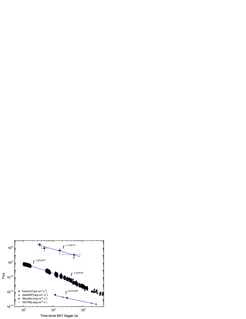
Figure 1: Multi-wavelength lightcurves of GRB 130907A. The best fit power-law (for $\gamma$-rays and optical band) or smoothly broken power-law (for X-rays) functions for the corresponding times (indicated by the start and end times of the lines) are shown. Flux from RATIR $i$-band observations were converted to the corresponding $I$-band flux following Blanton & Roweis (2007), to match the Skynet $I$-band observations.

The LAT light curve can be fitted with a single power law with a slope of $-$1.13$\pm$0.57 as shown in Fig. 1. Photon flux values are given here because energy flux depends largely on the photon indices that are sometimes not well constrained.

3.2 XRT data analysis

We extracted Swift/XRT lightcurve and spectra during the LAT observations using the standard HEASOFT reduction pipelines and the Swift/XRT repository (Evans et al., 2007; Evans et al., 2009). The XRT observations of GRB 130907A started in window timing (WT) mode and data were taken in the photon counting (PC) mode combined with WT mode since $\sim T_{\mathrm{0}}+$7000s. The PC spectrum can be fitted by an absorbed power-law model with a photon index 1.67$\pm$0.19 in the time interval from 3000 to 10000 seconds since $T_{\mathrm{0}}$, and 1.79$\pm$0.12 from 14000 to 20000 seconds since $T_{\mathrm{0}}$. The X-ray light curve can be fitted with a smoothed broken power law with a break at $\sim$19.6ks, the pre-break decay index is $-1.05\pm 0.07$, and the post-break decay index is $-2.43\pm 0.07$ as shown in Fig. 1.

4 Interpretations and Discussion

In this section, we will investigate the origin of the highest energy photon from GRB 130907A and assist the study by modeling the multi-band (from radio to GeV bands) data of this burst. Hereafter, we denote by $Q_{x}$ the value of the quantity $Q$ in units of $10^{x}$.

4.1 What is the origin of the highest energy photon above 10 GeV?

By equating the synchrotron cooling time in the magnetic field with the Lamour time of the electrons, one can obtain the Lorentz factors of the maximal energy electrons, which is $\gamma_{e,max}\propto B^{-1/2}$, where $B$ is the strength of the magnetic field. In the same magnetic field, the maximal synchrotron photon energy produced by these electrons is about 50 MeV in the shock co-moving frame. Considering the bulk motion boosting by the forward shock which has a Lorentz factor $\Gamma_{ext}(t)$, the maximal synchrotron photon energy is $\sim 50\Gamma_{ext}(t)$MeV. As the Lorentz factor of the forward shock decreases significantly at late times, one would expect $E_{max,syn}\lesssim 1.3(E_{54}/n_{0})^{1/8}T_{4}^{-3/8}$GeV. The presence of a 54.4GeV photon at $\sim T_{\mathrm{0}}+$5 hours is incompatible with a synchrotron origin even for the assumption about the fastest acceleration. It is more likely to originate from the inverse-Compton process, as also suggested by the detailed modeling of $>$10 GeV photons from GRB 130427A and other bursts (e.g. Wang et al. (2013); Liu et al. (2013)). The modeling of the broad-band SED, as shown in the following section, supports this explanation. Such a high-energy SSC emission has been predicted to be present in the high-energy afterglow emission for over a decade, e.g. Zhang & Mészáros (2001); Sari & Esin (2001).

4.2 The model

In the standard synchrotron afterglow spectrum, there are three break frequencies, $\nu_{a}$, $\nu_{m}$, and $\nu_{c}$, which are caused by synchrotron self-absorption, electron injection, and electron cooling, respectively. According to, e.g.  Sari et al. (1998) and  Wijers & Galama (1999), the cooling Lorentz factor and the minimum Lorentz factor of electrons in forward shocks are given by

$$\gamma_{m}=7.5\times 10^{2}f(p)\epsilon_{e,-1}E_{54}^{1/8}n_{0}^{-1/8}(1+z)^{3/8}T_{4}^{-3/8},$$ (1)

and

$$\gamma_{c}=3.5\times 10^{6}E_{54}^{-3/8}n_{0}^{-5/8}\epsilon_{B,-5}^{-1}(1+z)^{-1/8}(1+Y_{c})^{-1}T_{4}^{1/8},$$ (2)

where $E$ is the kinetic energy of the spherical shock, $\epsilon_{e}$ is the fraction of the shock energy that goes into the electrons, $\epsilon_{B}$ is fraction of the shock energy that goes into the magnetic fields, $n$ is the particle number density of the uniform medium, and $Y_{c}$ is the Compton parameter for electrons of energy $\gamma_{c}$ and $f_{p}=6(p-2)/(p-1)$), with $p$ being the electron index. These three characteristic frequencies are given by

$$\nu_{a}=8.9\times 10^{9}f^{-1}(p)\epsilon_{e,-1}^{-1}E_{54}^{1/5}n_{0}^{3/5}\epsilon_{B,-5}^{1/5}(1+z)^{-1}Hz,$$ (3)

$$\nu_{m}=1.2\times 10^{12}f^{2}(p)\epsilon_{e,-1}^{2}E_{54}^{1/2}\epsilon_{B,-5}^{1/2}(1+z)^{1/2}T_{4}^{-3/2}Hz,$$ (4)

and

$$\nu_{c}=2.5\times 10^{19}E_{54}^{-1/2}n_{0}^{-1}\epsilon_{B,-5}^{-3/2}(1+Y_{c})^{-2}(1+z)^{-1/2}T_{4}^{-1/2}Hz.$$ (5)

We can also get the peak flux of the synchrotron emission by

$$F_{\nu,m}=3.5\times 10^{4}E_{54}n_{0}^{1/2}\epsilon_{B,-5}^{1/2}D_{28}^{-2}(1+z)\mu{\rm Jy},$$ (6)

where $D$ is the luminosity distance. For the SSC emission, we get the corresponding quantities according to Sari & Esin (2001), i.e.

$$h\nu_{m}^{IC}=5.4f^{4}(p)\epsilon_{e,-1}^{4}E_{54}^{3/4}\epsilon_{B,-5}^{1/2}(1+z)^{5/4}T_{4}^{-9/4}{\rm keV},$$ (7)

$$h\nu_{c}^{IC}=2.5\times 10^{6}E_{54}^{-5/4}n_{0}^{-9/4}\epsilon_{B,-5}^{-7/2}(1+Y_{c})^{-4}(1+z)^{-3/4}T_{4}^{-1/4}{\rm TeV},$$ (8)

and

$$F_{\nu,m}^{IC}=5.6\times 10^{-3}E_{54}^{5/4}n_{0}^{5/4}\epsilon_{B,-5}^{1/2}D_{28}^{-2}(1+z)^{3/4}T_{4}^{1/4}\mu{\rm Jy}.$$ (9)

Due to the fact that the inverse-Compton scatterings between $\gamma_{c}$ electrons and the peak energy photons at frequency $\nu_{c}$ are typically in the Klein-Nishina (KN) regime, the SSC emission indeed peaks at

$$h\nu^{IC}_{peak}=\Gamma_{ext}m_{e}c^{2}\gamma_{c}=44(1+Y_{c})^{-1}E_{54}^{-1/4}n_{0}^{-3/4}\epsilon_{B,-5}^{-1}(1+z)^{1/4}T_{4}^{-1/4}{\rm TeV},$$ (10)

where $\Gamma_{ext}$ is the bulk Lorentz factor of the external forward shock. Above the peak $h\nu^{IC}_{peak}$, the spectrum has the form similar to Eq.50 in Nakar et al. (2009). In order to calculate $Y_{c}$, we need to consider the SSC emission in the KN scattering regime. Following Wang et al. (2010), we define a critical frequency, above which the scatterings with electrons of energy $\gamma_{c}$ just enter the KN scattering regime, i.e.

$$\nu_{{\rm KN}}(\gamma_{c})=8.7\times 10^{14}E_{54}^{1/2}n_{0}^{-1/2}\epsilon_{B,-5}^{-1/2}(1+Y_{c})(1+z)^{-1/2}T_{4}^{-1/2}Hz$$ (11)

In a broad parameter space, we find $\nu_{m}<\nu_{{\rm KN}}(\gamma_{c})<\nu_{c}$, thus following Wang et al. (2010), we have $Y_{c}(1+Y_{c})=\frac{\epsilon_{e}}{\epsilon_{B}}(\frac{\gamma_{c}}{\gamma_{m}})^{2-p}(\frac{\nu_{{\rm KN}}(\gamma_{c})}{\nu_{c}})^{(3-p)/2}$ (which is also consistent with eq. (47) in Nakar et al. 2009). Therefore, $Y_{c}$ is in the range from 4 to 6 in the time range between 1ks and 20ks after the burst for the reference parameter values of $\epsilon_{e,-1}=\epsilon_{B,-5}=E_{54}=n_{0}=1$.

4.3 Modeling the multi-wavelength emission

The multi-wavelength light curves are shown in Fig. 1. The X-ray light curves (3-10keV) initially decays as $t^{-1.05\pm 0.07}$ in the first 20ks and then steepens to a faster decay as $t^{-2.43\pm 0.07}$. The early X-ray decay slope $-1.05\pm 0.07$ and the spectral index $\beta_{\rm X}=0.67\pm 0.19$ are consistent with $\alpha=-(3p-3)/4$ and $\beta=-(p-1)/2$ ($F_{\nu}\propto t^{\alpha}\nu^{\beta}$) predicted by the standard afterglow synchrotron emission in the slow-cooling regime (i.e. $\nu_{m}<\nu_{\rm X}<\nu_{c}$) with $p\simeq 2.3$, assuming that the blast wave expands into a constant density circumburst medium. The wind medium scenario is not favored because the predicted decay slope in the wind medium scenario $\alpha_{w}=-(3p-1)/4$ is too steep. By fitting the I-band data from Skynet (Trotter et al., 2013b) and i-band data from RATIR (Butler et al., 2013a, b; Lee et al., 2013, converted to I-band data according to Blanton & Roweis, 2007), we got the decay slope $-0.87\pm 0.09$, which is consistent with $\sim$0.9 in Trotter et al. (2013b). The decay slope is consistent with the predicted slope $\alpha=-(3p-3)/4$ when the optical frequency $\nu_{\rm O}$ also locates at $\nu_{m}<\nu_{\rm O}<\nu_{c}$. It is puzzling that the optical light curve does not show a break as X-rays. We speculate that there might be some extra contribution to the late-time optical flux, such as the host galaxy or another possible outflow component. Such chromatic break behavior has been seen before in other GRBs as well, e.g. Panaitescu et al. (2006).

The LAT emission decays as $t^{-1.13\pm 0.57}$ with a large error bar in the decay slope due to small number of high-energy photons. The decay slope is consistent with the predicted slope $\alpha=-(3p-2)/4$, as the LAT energy window is above the cooling frequency $\nu_{c}$. Note that the time evolution of the Compton parameter (defined as $Y(\gamma_{*})$ in  Wang et al. (2010)) for the high-energy emission could steepen the LAT synchrotron decaying light curve, since the high-energy synchrotron flux scales as $1/(1+Y(\gamma_{*}))$. The value of $Y(\gamma_{*})$ is $\simeq 2$ at a few ks. However, because the measured decay slope has a large error (i.e. $-1.13\pm 0.57$), such effect is hard to be discerned from the data.

Below we model the multi-band SED with the synchrotron plus SSC emission model.

The LAT flux at $h\nu=100$ MeV is about $(6.0\pm 3.3)\times 10^{-4}\mu{\rm Jy}$ around 6000s after the burst. Since at $h\nu=100{\rm MeV}$ the flux is dominated by the synchrotron emission, we have

$$F_{\nu}({\rm 100{\rm MeV}},t=6{\rm ks})=F_{\nu,m}(\frac{\nu_{c}}{\nu_{m}})^{-(p-1)/2}(\frac{100{\rm MeV}}{h\nu_{c}})^{-p/2}=(6.0\pm 3.3)\times 10^{-4}\mu{\rm Jy}.$$ (12)

The X-ray flux density at 1 keV around 17ks is about $(11.6\pm 2.1)\mu{\rm Jy}$ which was derived from the Swift XRT data, as discussed above, and we have

$$F_{\nu}(1{\rm keV},t=17{\rm ks})=F_{\nu,m}(\frac{1{\rm keV}}{h\nu_{m}})^{-(p-1)/2}=(11.6\pm 2.1)\mu{\rm Jy}.$$ (13)

VLA observations started at $\sim T_{\mathrm{0}}+$14ks and ended at $\sim T_{\mathrm{0}}+$20ks at $\nu=24.5$GHz, the flux is ($1.2\pm 0.09$)mJy (Corsi, 2013). Since the high frequency of radio band locates between the self-absorption frequency $\nu_{a}$ and $\nu_{m}$, we have

$$F_{\nu}(24.5{\rm GHz},t=4{\rm hr})=F_{\nu,m}(\frac{24.5{\rm GHz}}{\nu_{m}})^{1/3}\simeq(1.2\pm 0.09)m{\rm Jy}.$$ (14)

The flux at 10GeV at 17000s after the burst should be dominated by the SSC emission as discussed above. With a flux of (1.75$\pm$1.48) $\times 10^{-5}\mu{\rm Jy}$ at 10 GeV, we have ($h\nu_{m}^{IC}$¡10GeV$<h\nu_{c}^{IC}$)

$$F_{\nu}(10{\rm GeV},t=17{\rm ks})=F_{\nu,m}^{IC}(\frac{10{\rm GeV}}{h\nu_{m}^{IC}})^{-(p-1)/2}=(1.75\pm 1.48)\times 10^{-5}\mu{\rm Jy}.$$ (15)

We find that the following parameter values are consistent with the observed data: $E_{54}=0.75$, $\epsilon_{e,-1}=3.2$, $\epsilon_{B,-5}=0.55$, $n={\rm 1.8cm^{-3}}$. The obtained value of $\epsilon_{B}$ is quite small and the obtained value of the kinetic energy implies a very large efficiency in producing gamma-rays. For these parameter values, we find that $Y_{c}$ is about 12-16 in the time between 1ks and 20ks after the burst, and the assumption ${\nu_{m}}<{\nu_{KN}(\gamma_{c})}<{\nu_{c}}$ holds in this time range. Since in our case the forward shock electrons are in the slow-cooling regime (i.e. $\gamma_{m}<\gamma_{c}$), $Y_{c}$ roughly reflects the total luminosity ratio between the SSC component and the synchrotron component (Nakar et al., 2009). The fluence emitted by the SSC component can be estimated from the spectral energy distribution in Fig.2, which is roughly $F\sim 2\times 10^{-5}{\rm erg\,cm^{-2}}$, so the energy radiated in the SSC component is about $8\times 10^{52}{\rm erg}$. The fluence in the synchrotron component is about a factor of 10 smaller than the SSC component, consistent with the estimated value of $Y_{c}$. Thus, the total energy in the afterglow emission is about one order of magnitude lower than the inferred kinetic energy of the forward shock, which is $E=7.5\times 10^{53}{\rm erg}$.

Guided by the above parameter values, we model the multi-band SED with the synchrotron plus SSC emission model, as shown in Fig. 2. For the synchrotron component, we use a series of smoothly connected power-laws with two breaks at $\nu_{m}$ and $\nu_{c}$ as well as an exponential cutoff at $E_{\mathrm{max,syn}}$. And for the SSC component, we use a series of smoothly connected power-laws with breaks at $\nu_{m}^{IC}$ and $\nu_{peak}^{IC}$. The results favor that the $>10$ GeV emission is produced by the SSC component.

4.4 Discussions

Fermi/LAT has detected long-lasting high-energy photons (¿100 MeV) from about 60 gamma-ray bursts (GRBs) as of Feb 2014 , with the highest energy photons reaching about 100 GeV. One widely discussed scenario is that this emission is the afterglow synchrotron emission produced by electrons accelerated in the forward shocks. It has been pointed out that, although this scenario can explain the extended 100MeV-GeV emission very well, it has difficulty in explaining $>10$ GeV photons, especially in the late afterglow, since the maximum synchrotron photon energy is limited  (Piran & Nakar, 2010; Barniol Duran & Kumar, 2011; Sagi & Nakar, 2012; Wang et al., 2013). The late $>10$ GeV emission could in principle be produced by the afterglow SSC emission, as indeed has been invoked to explain the late $>10$ GeV emission in e.g. GRB130427A  (Tam et al., 2013; Fan et al., 2013; Liu et al., 2013; Panaitescu et al., 2013) and GRB090926A (Wang et al., 2013).

In this paper, we report the analysis of the Fermi/LAT observations of GRB 130907A  and the detection of one 55 GeV photon compatible with the position of GRB 130907A  at about 5 hours after the burst. The probability that this photon is associated with GRB 130907A  was found to be higher than 99.96%. At this late time, the energy of this photon exceeds the maximum synchrotron photon energy. We modeled the broad-band SED of the afterglow emission and find that this high energy photon is consistent with the SSC emission of the afterglow.

Table 1: LAT analysis results of GRB 130907A.

Time since $T_{0}$	Energy	TS value	$\Gamma$	Flux
(s)	(GeV)			(10-7 ph cm2 s-1)
3000–4000	0.1–60	23.1	2.4$\pm$0.5	29.0$\pm$14.9
4000–6000	0.1–60	16.4	2.3$\pm$0.6	9.2$\pm$5.4
14000–20000	0.1–60	24.3	2.0(1.5)	4.5$\pm$3.3(2.3$\pm$2.0)
3000–6000	0.1–0.2	9.5	3.4$\pm$1.7	6.9$\pm$4.0
…	0.2–0.5	10.0	2.0(1.5)	3.4$\pm$1.0(3.3$\pm$0.8)
…	0.5–1.1	10.0	2.0(1.5)	1.7$\pm$1.1(1.6$\pm$1.1)
…	1.1–60	0.0	2.0(1.5)	$<$1.0($<$1.0)
14000–20000	0.1–0.5	0.8	2.0(1.5)	$<$11.8($<$11.3)
…	0.5–1.1	0.0	2.0(1.5)	$<$0.9($<$0.9)
…	1.1–60	27.7	2.0(1.5)	0.6$\pm$0.5(0.6$\pm$0.5)

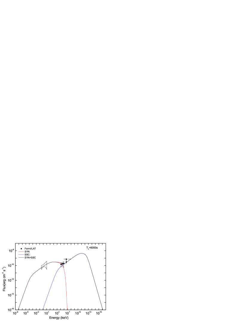
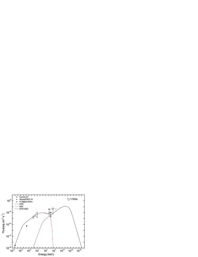
Figure 2: The broadband SEDs at around 6000s (upper panel) and 17000s (lower panel) after the burst. The LAT data points were derived from observations during 3ks–6ks and 14ks–20ks after $T_{0}$, respectively, as presented in Table 1. Upper limits assuming $\Gamma=2.0$ are shown. The butterflies represent the best-fit spectra in the 0.3-10 keV range derived from the absorbed power-law model in two time intervals after $T_{0}$: 3ks–10ks and 14ks–20ks. Optical and radio flux are taken from Skynet (Trotter et al., 2013a, b) and VLA (Corsi, 2013) observations, respectively. The red and blue dotted lines represent the model synchrotron component and SSC component respectively and the black solid lines represent the sum of them. Discrepancy between the optical ($I$ band) data and the model flux in the bottom panel can be accounted for by the extinction of the host galaxy using the column density given in the XRT fits. The model lines are calculated based on the following parameter values: $E=0.5\times 10^{54}$ ergs, $\epsilon_{e}=0.35$, $\epsilon_{B}=0.44\times 10^{-5}$, $n=1.78cm^{-3}$. Note that the parameter values here are slightly different from those in the text because smoothed broken power-law functions, instead of power-law functions with sharp breaks, are used for the fit of the synchrotron and SSC spectra of the SED shown here.

References

- Ackermann et al. (2013) Ackermann, M., Ajello, M., Asano, K., et al. 2013, ApJS, 209, 11
- Ackermann et al. (2014) Ackermann, M., Ajello, M., Asano, K., et al. 2014, Science, 343, 42
- Atwood et al. (2013) Atwood, W. B., Baldini, L., Bregeon, J., et al. 2013, ApJ, 774, 76
- Barniol Duran & Kumar (2011) Barniol Duran, R., & Kumar, P. 2011, MNRAS, 412, 522
- Blanton & Roweis (2007) Blanton, M. R., & Roweis, S. 2007, AJ, 133, 734
- Burrows et al. (2013) Burrows, D. N., Kennea, J. A., Evans, P. A., et al. 2013, GRB Coordinates Network, 15199, 1
- Butler et al. (2013a) Butler, N., Watson, A. M., Kutyrev, A., et al. 2013, GRB Coordinates Network, 15208, 1
- Butler et al. (2013b) Butler, N., Watson, A. M., Kutyrev, A., et al. 2013, GRB Coordinates Network, 15209, 1
- Corsi (2013) Corsi, A. 2013, GRB Coordinates Network, 15200, 1
- de Ugarte Postigo et al. (2013) de Ugarte Postigo, A., Xu, D., Malesani, D., et al. 2013, GRB Coordinates Network, 15187, 1
- Evans et al. (2007) Evans, P. A., Beardmore, A. P., Page, K. L., et al. 2007, A&A, 469, 379
- Evans et al. (2009) Evans, P. A., Beardmore, A. P., Page, K. L., et al. 2009, MNRAS, 397, 1177
- Fan et al. (2013) Fan, Y.-Z., Tam, P. H. T., Zhang, F.-W., et al. 2013, ApJ, 776, 95
- Ghisellini et al. (2010) Ghisellini, G., Ghirlanda, G., Nava, L., & Celotti, A. 2010, MNRAS, 403, 926
- Golenetskii et al. (2013) Golenetskii, S., Aptekar, R., Frederiks, D., et al. 2013, GRB Coordinates Network, 15203, 1
- He et al. (2011) He, H. N., Wu, X. F., Toma, K., Wang, X. Y., & Mészáros, P. 2011, ApJ, 733, 22
- Hurley et al. (1994) Hurley, K., Dingus, B. L., Mukherjee, R., et al. 1994, Nature, 372, 652
- Kumar & Barniol Duran (2009) Kumar, P., & Barniol Duran, R. 2009, MNRAS, 400, L75
- Kumar & Barniol Duran (2010) Kumar, P., & Barniol Duran, R. 2010, MNRAS, 409, 226
- Lee et al. (2013) Lee, W. H., Butler, N., Watson, A. M., et al. 2013, GRB Coordinates Network, 15192, 1
- Liu et al. (2013) Liu, R.-Y., Wang, X.-Y., & Wu, X.-F. 2013, ApJ, 773, L20
- Mattox et al. (1996) Mattox, J. R., Bertsch, D. L., Chiang, J., et al. 1996, ApJ, 461, 396
- Mészáros & Rees (1994) Mészáros, P., & Rees, M. J. 1994, MNRAS, 269, L41
- Nakar et al. (2009) Nakar, E., Ando, S., & Sari, R. 2009, ApJ, 703, 675
- Nolan et al. (2012) Nolan, P. L., Abdo, A. A., Ackermann, M., et al. 2012, VizieR Online Data Catalog, 219, 90031
- Page et al. (2013) Page, M. J., Beardmore, A. P., Burrows, D. N., et al. 2013, GRB Coordinates Network, 15183, 1
- Panaitescu et al. (2006) Panaitescu, A., Mészáros, P., Burrows, D., Nousek, J., Gehrels, N., O’Brien, P., & Willingale, R. 2006, MNRAS, 369, 2059
- Panaitescu et al. (2013) Panaitescu, A., Vestrand, W. T., & Woźniak, P. 2013, MNRAS, 436, 3106
- Piran & Nakar (2010) Piran, T., & Nakar, E. 2010, ApJ, 718, L63
- Sagi & Nakar (2012) Sagi, E., & Nakar, E. 2012, ApJ, 749, 80
- Sari & Esin (2001) Sari, R., & Esin, A. A. 2001, ApJ, 548, 787
- Sari et al. (1998) Sari, R., Piran, T., & Narayan, R. 1998, ApJ, 497, L17
- Savchenko et al. (2013) Savchenko, V., Beckmann, V., Ferrigno, C., et al. 2013, GRB Coordinates Network, 15204, 1
- Tam et al. (2013) Tam, P.-H. T., Tang, Q.-W., Hou, S.-J., Liu, R.-Y., & Wang, X.-Y. 2013, ApJ, 771, L13
- Trotter et al. (2013a) Trotter, A., Haislip, J., Lacluyze, A., et al. 2013, GRB Coordinates Network, 15191, 1
- Trotter et al. (2013b) Trotter, A., Reichart, D., Haislip, J., et al. 2013, GRB Coordinates Network, 15193, 1
- Vianello et al. (2013) Vianello, G., Kocevski, D., Racusin, J., & Connaughton, V. 2013, GRB Coordinates Network, 15196, 1
- Wang et al. (2010) Wang, X.-Y., He, H.-N., Li, Z., Wu, X.-F., & Dai, Z.-G. 2010, ApJ, 712, 1232
- Wang et al. (2013) Wang, X.-Y., Liu, R.-Y., & Lemoine, M. 2013, ApJ, 771, L33
- Wijers & Galama (1999) Wijers, R. A. M. J., & Galama, T. J. 1999, ApJ, 523, 177
- Xue et al. (2009) Xue, R. R., Tam, P. H., Wagner, S. J., et al. 2009, ApJ, 703, 60
- Zhang & Mészáros (2001) Zhang, B., & Mészáros, P. 2001, ApJ, 559, 110
- Zou et al. (2009) Zou, Y.-C., Fan, Y.-Z., & Piran, T. 2009, MNRAS, 396, 1163