The D0 Collaboration111with visitors from aAugustana College, Sioux Falls, SD, USA, bThe University of Liverpool, Liverpool, UK, cDESY, Hamburg, Germany, dUniversidad Michoacana de San Nicolas de Hidalgo, Morelia, Mexico eSLAC, Menlo Park, CA, USA, fUniversity College London, London, UK, gCentro de Investigacion en Computacion - IPN, Mexico City, Mexico, hUniversidade Estadual Paulista, São Paulo, Brazil, iKarlsruher Institut für Technologie (KIT) - Steinbuch Centre for Computing (SCC), D-76128 Karlsruhe, Germany, jOffice of Science, U.S. Department of Energy, Washington, D.C. 20585, USA, kAmerican Association for the Advancement of Science, Washington, D.C. 20005, USA, lKiev Institute for Nuclear Research, Kiev, Ukraine, mUniversity of Maryland, College Park, Maryland 20742, USA, and nLaboratoire de Physique Theorique, Orsay, FR.
Measurement of the forward–backward asymmetry in
top quark–antiquark production in collisions using the lepton+jets channel
Abstract
We present a measurement of the forward–backward asymmetry in top quark–antiquark production using the full Tevatron Run II dataset collected by the D0 experiment at Fermilab. The measurement is performed in lepton+jets final states using a new kinematic fitting algorithm for events with four or more jets and a new partial reconstruction algorithm for events with only three jets. Corrected for detector acceptance and resolution effects, the asymmetry is evaluated to be . Results are consistent with the standard model predictions which range from 5.0% to 8.8%. We also present the dependence of the asymmetry on the invariant mass of the top quark–antiquark system and the difference in rapidities of top quark and antiquark.
pacs:
14.65.Ha,12.38.Qk,11.30.Er,13.85.-tI Introduction
I.1 Motivation and definitions
Over the last five years both experiments at the Fermilab Tevatron Collider measured positive forward–backward asymmetries in the production of top quark–antiquark pairs in proton–antiproton collisions () bib:p17PRL ; bib:CDFPRL ; bib:CDFdep ; bib:ourPRD ; bib:CDF2012 . The reported values were consistently above predictions of the standard model of particle physics (SM) bib:KnR ; bib:other . In particular, the CDF Collaboration observed a strong rise of the asymmetry with the invariant mass of the system, bib:CDFdep . The dependence of the asymmetry on in D0 data, as measured in Ref. bib:ourPRD , was statistically compatible with both the SM predictions and with the CDF result. Several beyond-the-SM scenarios were suggested to explain the measured values bib:BSM , in particular using the framework of parity-violating strong interactions suggested in Ref. bib:axigluon . In this paper we report new results from the D0 experiment based on the full dataset collected during Run II of the Fermilab Tevatron Collider, which supersede the result of Ref. bib:ourPRD .
In proton–antiproton collisions, top quark–antiquark pairs are predominantly produced via valence quark–antiquark annihilation. Thus, the direction of the proton (antiproton) almost always coincides with the direction of the incoming quark (antiquark). We define the difference in rapidity222 The rapidity is defined as , where is the particle’s energy and is its momentum along the -axis, which corresponds to the direction of the incoming proton. between the top quark () and antiquark ():
| (1) |
We refer to the events that have as “forward”, and to those with as “backward”. The forward–backward asymmetry in production is defined as
| (2) |
where () is the number of forward (backward) events. All asymmetries reported in this paper are given after subtracting the contributions from background processes.
The rapidities of the and quarks and the corresponding asymmetries can be defined at the production level (sometimes denoted as generator level or parton level), when the kinematic parameters of the generated top quarks are used. Unless stated otherwise the production-level asymmetries are defined for all signal events without imposing the selection criteria of this analysis. The rapidities and asymmetry can also be defined at the reconstruction level, using the reconstructed kinematics of the selected events. Similarly, the invariant mass of the system can be defined at the production and reconstruction levels.
I.2 Strategy
In the SM a top quark almost always decays to a quark and a boson, which decays either leptonically or hadronically. In this paper we identify events using the ; ; (and charge conjugates) decay chain. This channel is commonly referred to as the “lepton+jets” () channel. We select events that contain one isolated lepton (electron or muon) of high transverse momentum () and at least three jets. The electric charge of the lepton identifies the electric charge of the leptonically decaying boson and its parent top quark. The other top quark is assumed to have the opposite charge. The event selection, sample composition determination, and modeling of the signal and background processes are identical to those used in the measurement of the leptonic asymmetry in production in the channel bib:our_afbl . The four-vectors of the top quarks and antiquarks in the events containing at least four jets are reconstructed with a kinematic fitting algorithm, while for the events that contain only three jets a partial reconstruction algorithm is used. If a jet exhibits properties consistent with a jet originating from a quark, such as the presence of a reconstructed secondary vertex, we identify it as a -tagged jet bib:btagging . The events are separated into channels defined by jet and -tag multiplicities. The amount of signal and the forward–backward asymmetry at the reconstruction level are determined using a simultaneous fit to a kinematic discriminant in these channels.
The measured background/subtracted one/dimensional (1D) distribution in is corrected to the production level (“unfolded”). From this distribution we calculate the fully/corrected as well as its dependence on . To study the dependence of the asymmetry on the invariant mass of the system, unfolding is done on the background-subtracted data distributions in two dimensions (2D: vs ). The signal channels are unfolded simultaneously to yield the desired 1D or 2D production/level distributions, from which the production/level values are computed using Eq. 2. The procedure is calibrated using simulated samples with varied asymmetries and input distributions in and . The statistical and systematic uncertainties of the results are evaluated using ensembles of simulated pseudo/datasets (PDs).
II D0 detector
We use the data collected by the D0 detector during Run II of the Tevatron in the years 2001–2011. After imposing event quality requirements ensuring that all detector systems were fully operational, this dataset corresponds to an integrated luminosity of . The D0 detector is described in detail elsewhere bib:D0det . The central tracking system, consisting of a silicon microstrip tracker and a scintillating fiber tracker, is enclosed within a T superconducting solenoid magnet. Tracks of charged particles are reconstructed within a detector pseudorapidity region333The detector pseudorapidity is defined as , where is the polar angle measured with respect to the center of the detector. The angle corresponds to the direction of the incoming proton. of . Electrons, photons, and jets of hadrons are identified bib:ehadID using a liquid-argon and uranium-plate calorimeter, which consists of a central barrel covering up to , and two endcap sections that extend coverage to bib:run1det . Central and forward preshower detectors are positioned in front of the corresponding sections of the calorimeter. A muon system consisting of layers of tracking detectors and scintillation counters placed in front of and behind T iron toroids bib:run2muon identifies muons bib:muID within . Luminosity is measured using arrays of plastic scintillators located in front of the endcap calorimeter cryostats. A three-level trigger system selects interesting events at the rate of Hz for offline analysis bib:D0trig .
III Event selection and modeling
Object reconstruction and identification, as well as event selection, are the same as in Ref. bib:our_afbl and are briefly outlined in this section. We select events with exactly one isolated electron within the detector pseudorapidity range of or one isolated muon within , and at least three jets within . To limit the possible contribution of poorly modeled background due to multijet production, leptons of either flavor are required to have . The presence of a neutrino is inferred from a transverse momentum imbalance, which is measured primarily using calorimetry and is referred to as the “missing transverse energy” . All selected objects are required to have transverse momentum GeV, and the jet with the largest (the leading jet) is also required to have GeV.
To identify jets that are likely to be associated with quarks, we perform a multivariate analysis (MVA) that combines variables characterizing the properties of secondary vertices and of tracks with large impact parameters relative to the primary interaction vertex (PV) bib:btagging . The output of the MVA is a continuous variable, . The requirement on ( tagging) used in this analysis has an efficiency of about 64% for identifying jets originating from top quark decay, and a misidentification probability of about 7% for jets that do not contain heavy flavor quarks and are produced in association with leptonically decaying bosons.
We simulate production using MC@NLO program (version 3.4) bib:mcatnlo with the parton showering performed by HERWIG bib:herwig . This simulation is fully integrated with the D0 software, allowing for detailed studies of the kinematic dependences of and their interplay with selection and reconstruction effects. The main source of background to the signal is the production of a leptonically decaying boson in association with jets (jets). The kinematic properties of this process are simulated using ALPGEN bib:alpgen with hadronic showering performed by PYTHIA bib:pythia . For signal and background modeling we use the CTEQ6.1 set of parton distribution functions (PDFs) bib:CTEQ . The normalization of the jets contribution is a free parameter in the fitting procedure described below. Events with multiple jets can also mimic signal when a particle from one of the jets is misidentified as an isolated lepton. The normalization of this multijet background is extrapolated from a control sample enriched in this process using the probability for a jet to satisfy the lepton-quality requirements bib:matrix_method . For the other backgrounds, +jets events are simulated with ALPGEN, diboson events are simulated with PYTHIA, and events from single-top-quark production are simulated with COMPHEP bib:comphep . The normalizations for the last three background processes are taken from NLO calculations bib:mcfm . In all cases, event generation is followed by the GEANT/based D0 detector simulation bib:geant . To model energy depositions from noise and additional collisions within the same bunch crossing, simulated events are overlaid with data from random crossings. All simulated events are reconstructed using the same code as for the reconstruction of the collider data.
IV Reconstruction of the event kinematics
To measure the forward–backward asymmetry and its dependence on the invariant mass of the system we need to determine the four-vectors of top quark and antiquark, which is done by summing the four-vectors of their decay products in the ; ; (and charge conjugates) decay chain. There are four final state quarks in this decay chain, while we select events that contain one isolated lepton and at least three jets. When an event contains at least four jets we assume that the four jets with the largest originate from the quarks from decay. If an event contains only three jets one of the jets from decay is missing. In either case all possible assignments of three or four jets to the final state quarks are used, with the likelihood of each assignment evaluated by the reconstruction algorithms described below.
For +4 jet events, the system is fully reconstructed using a kinematic fitting algorithm. Previous D0 top quark analyses used the algorithm of Ref. bib:hitfit . In this paper a new algorithm is employed, which utilizes an analytic solution for the neutrino momentum using the constraints on the -boson () and top-quark masses () bib:analytical . The likelihood term for each jet-to-quark assignment accounts for the differences between the observed jet energy and the energy scaled to satisfy the constraints on and . The jet energy resolution and the probability for a jet to be reconstructed (see “Type III” transfer function in Ref. bib:transfer_funcs ) are taken into account. The -tagging observables are also used to evaluate the likelihood of each assignment.
For events, a partial reconstruction algorithm of the decay chain is employed bib:NIM_3j . With one jet entirely lost, no significant improvement is expected from scaling the four-vectors of the remaining objects as is done by the kinematic fitting algorithm in +4 jet events, so the partial reconstruction algorithm does not attempt to modify the kinematics of the observed objects. As only the transverse components of the neutrino momentum are measured in , the longitudinal component is calculated using a quadratic equation which results from imposing the constraint on the decay products. The two-fold ambiguity is resolved by choosing the solution that minimizes the difference between the known and the invariant mass of the objects assigned to the leptonic top quark decay, . This algorithm thus assumes that the jet associated with the quark from the leptonically decaying top quark is detected. This assumption holds for 80% of the events. The lost jet is assumed to be associated with either a light quark or a quark from the hadronic top-quark decay chain. In the majority of cases (74%) this jet is lost due to its low energy, so this loss has little effect on the kinematics of the hadronically decaying top quark. The lost jet is neglected in the partial reconstruction algorithm. The sum of the four-vectors of the two jets assigned to the products of the hadronically decaying top quark serves as a proxy for the four-vector of the hadronically decaying top quark with the invariant mass . Even though is not expected to be equal to , the distribution in this variable is different for combinations correctly associated with the hadronically decaying top quark and combinations that include a jet from the leptonically decaying top quark. In each event we consider the following nine observables: the for each of the three jets, the three possible , corresponding to the three possible lepton-neutrino-jet combinations, and the three possible . The likelihood of each of the three possible jet-to-quark assignment is calculated by evaluating the consistency of the nine observables with the distributions corresponding to the hypothesized assignment. In particular, the jet hypothesized to be associated with a quark should have a value of consistent with the one expected for jets, while for a jet hypothesized to originate from a boson decay should be consistent with the distribution expected for such jets. The values of and for the jet combinations that correspond to the hypothesized assignment should be consistent with the distributions expected for correctly assigned jets, while the values of and for the other jet combinations should agree with the distributions expected for wrong assignments. When calculating , we compensate for the effect of the lost jet by applying an -dependent scaling to the four-vector of the hadronically decaying top quark.
Unlike the measurement in Ref. bib:ourPRD , where only the jet-to-quark assignment with the lowest was used, we reconstruct by averaging its values over all possible assignments, weighted by their likelihoods evaluated as described above for +4 jet and events. The same approach is used to reconstruct in the channel. For +4 jet events, is reconstructed using the outputs of three reconstruction algorithms: the new kinematic fit algorithm, the kinematic fit algorithm of Ref. bib:hitfit , and a simple reconstruction algorithm bib:ttres that evaluates the kinematics of the leptonically decaying boson from the lepton and the neutrino by imposing the constraint and calculates by adding the four most energetic jets without imposing the constraint. The likelihood values calculated by the algorithms give indications on how well the kinematics of a particular event match the assumptions made by a given algorithm. In particular, for high there is a higher probability that two final state quarks are associated with the same jet. Such a jet is likely to be the most energetic jet in the event and have a large mass. The simple reconstruction algorithm, which does not assume a specific jet-to-quark assignment, performs best for such events. We use a multivariate regression TMVA2007 to combine the partially correlated values and the likelihoods produced by the three algorithms with supplementary observables such as the mass of the leading jet to estimate . This combined reconstruction outperforms the individual algorithms in all ranges.
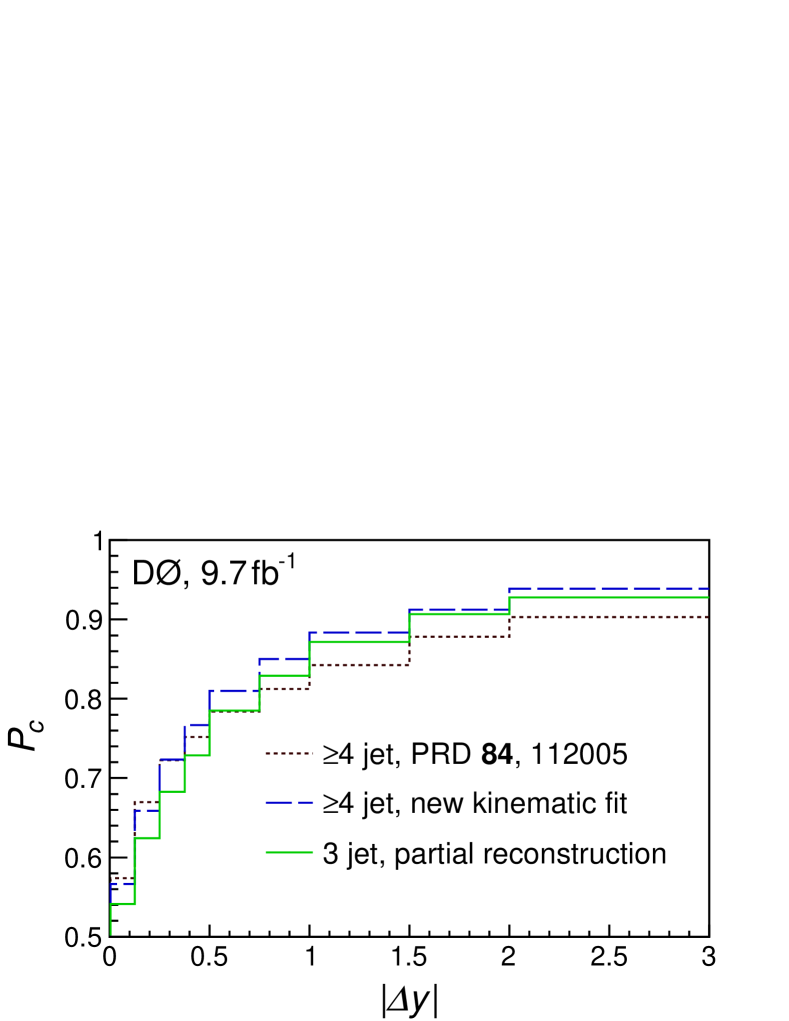
For the asymmetry measurement the performance of a reconstruction algorithm can be characterized by the probability to correctly reconstruct the sign of . For the algorithm employed in this analysis for +4 jet events , compared to for the algorithm of Ref. bib:hitfit . The partial reconstruction algorithm achieves for events. The dependence of on the production/level is shown in Fig. 1 for these three algorithms. The high values of achieved by the partial reconstruction algorithm, which are almost as high as for +4 jet events, can be understood from the following consideration. All four leading jets are associated with the quarks from the decay in only 55% of the +4 jet events. For the other 45% of the events one of the jets originates from initial or final state radiation, which can lead to badly misreconstructed four-vectors. Only 4% of the events contain a jet that does not originate from the four quarks of the decay. Thus, even though some information is lost with the unreconstructed jet, no wrong information is added, leading to a low probability to misreconstruct the sign of .
V SM predictions for
The differential cross section for production is available only at order , where is the strong coupling constant. Since in the SM the asymmetry only appears at this order, no full higher order prediction for exists yet. The relative uncertainty on the calculation of the asymmetry due to higher order corrections is evaluated to be as large as bib:Bern .
Recently the order calculation for the total cross section of production bib:Mitov was made available, but the asymmetry was not computed at this order. Several papers report calculations of the leading corrections to the asymmetry with the predicted values ranging from in MC@NLO to once the electroweak corrections bib:EWcorr and resummations of particular regions of phase space bib:resummed_afb are taken into account. The dominant uncertainty on these predictions is from the renormalization and factorization scales, and is evaluated to be as high as (absolute) bib:MCFMttbar ; bib:Bern . The authors of Ref. bib:PMC_scale obtain a value of by choosing a normalization scale that arguably stabilizes the perturbative expansion yet differs significantly from the scales commonly used in top quark physics calculations. Some authors suggest that the corrections from interactions between the top quark decay products and the proton remnants should also be taken into account when calculating bib:rescat . Given this variety of predictions, we choose to compare our data to the well defined MC@NLO simulation.
At order , the QCD contributions to the asymmetry in production can be divided into two classes up to divergences that cancel between these two classes bib:KnR . The first class, which contributes to negative asymmetry, is a result of interference between the terms that contain gluon radiation in the initial or final states, which may result in an extra jet in the event and typically leads to a higher transverse momentum of the system. The second class, which contributes to positive asymmetry, is from interference between the Born term () and the term described by a box diagram (). The overall asymmetry is positive and depends on the jet multiplicity. Selection criteria that give preference to events with higher jet multiplicity favor the first class of events and further lower the overall expected asymmetry, while a higher asymmetry is expected for events with lower jet multiplicity. Consequently, forward events tend to have fewer jets than events in the backward category. Similarly, since a -tagged jet is less likely to originate from initial or final state radiation, samples with a larger number of tags tend to have higher values of .
MC@NLO predicts an overall asymmetry in production before selection of %. Here, and in the following sections, the quoted uncertainties on the predictions are from the finite size of the simulated samples unless otherwise stated. Table 1 lists the MC@NLO predictions for events after the selection criteria are applied.
All previous measurements of in the channel selected events that had at least four jets in the final state. As is apparent from Table 1, restricting the selection to only +4 jet events lowers the production/level asymmetry. Including events with three jets reduces this selection bias.
| , % | ||
| Channel | Production | Reconstruction |
| level | level | |
| 3 jets, 1 tags | ||
| 3 jets, tag | ||
| 3 jets, 2 tags | ||
| 4 jets, tag | ||
| 4 jets, 2 tags | ||
Asymmetries after reconstruction are presented in the last column of Table 1. Finite resolution in results in roughly of the forward events being misreconstructed as backward, and vice versa. Since there are more forward events, smearing leads to an overall lowering of the reconstructed asymmetries. At the same time, forward events, which tend to have fewer jets, have a lower probability to be misreconstructed, resulting in fewer migrations into the backward category, and an upward shift in the reconstructed asymmetry. This bias is most apparent in the +4 jet, one--tag channel, where the lowest asymmetry is predicted.
VI Sample Composition and Reconstruction/level
Reconstructed events are divided into six channels by the number of jets and tags: and +4 jet with 0, 1, and 2 tags each. The zero--tag channel is used only for the background asymmetry calibration, and not for the asymmetry measurement. The +4 jet zero--tag channel is used only for determining the sample composition and the reconstruction/level , and is not used for measuring the production/level asymmetry.
Several well-modeled variables that have different distributions for signal and background processes, and that have minimal correlations between each other and with and , are combined into kinematic discriminants bounded between 0 and 1 bib:our_afbl . For +4 jet events a discriminant is built from the following input variables:
-
•
– the test statistic of the likeliest assignment from the kinematic fit.
-
•
– the transverse momentum of the leading -tagged jet, or when no jets are tagged, the of the leading jet.
-
•
, where is the angular distance444Here the pseudorapidity and the azimuthal angle are defined relative to the PV. between the two closest jets, and , and and are their transverse momenta.
-
•
, the invariant mass of the jets corresponding to the decay in the likeliest assignment from the kinematic fit, calculated using kinematic quantities before the fit.
The variables and are based on the full reconstruction using the kinematic fitting technique of Ref. bib:hitfit .
For the events we construct a discriminant using a different set of input variables:
-
•
— the sphericity bib:spher , defined as , where and are the two largest of the three eigenvalues of the normalized quadratic momentum tensor . The tensor is defined as
(3) where is the momentum vector of a reconstructed object , and and run over the three indices for the Cartesian coordinates. The sum over objects includes the three selected jets and the selected charged lepton.
-
•
— the transverse momentum of the third leading jet.
-
•
— the lowest of the invariant masses of two jets, out of the three possible jet pairings.
-
•
, defined as for the +4 jet channel, above.
-
•
, the difference in azimuthal angle between the leading jet and .
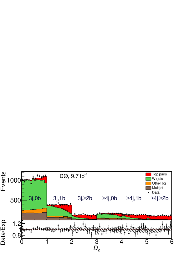
The discriminants for all channels are combined into a single discriminant , so that for the events , while for +4 jet events . The variable above is usually taken to be equal to the number of -tagged jets in the event, but for events with more than two -tagged jets instead. We fit the sum of the signal and background templates to the data distribution in the discriminant as shown in Fig. 2. This fit is identical to the fit for the sample composition in Ref. bib:our_afbl . The sample composition and its breakdown into individual channels are summarized in Table 2. Background contributions other than jets and multijet production are labeled “Other Bg” in Table 2.
| Selected | 3 jets | 4 jets | |||
|---|---|---|---|---|---|
| Source | events | tag | 2 tags | tag | 2 tags |
| jets | |||||
| Multijet | |||||
| Other Bg | 786 | ||||
| Signal | |||||
| Sum | 10947 | 4526 | 1560 | 1588 | 1339 |
| Data | 10947 | 4588 | 1527 | 1594 | 1281 |
In the simulated jets background, the angular distribution of leptons from -boson decay has a forward–backward asymmetry, which is in part tuned to Tevatron data bib:CDFWasym . Due to this asymmetry, when these events are reconstructed according to the hypothesis, there remains a residual asymmetry of in the distribution. To improve the modeling of this asymmetry, we apply a weight to each simulated jets event which depends on the product of the generated lepton charge and its rapidity. These weights are chosen so that the simulation best matches control data with three jets and zero tags as in Ref. bib:our_afbl . The difference in the distributions predicted by the simulation with and without the applied weights is treated as a source of systematic uncertainty due to background modeling. This uncertainty exceeds the uncertainty due to PDFs by about a factor of two. We rely on the simulation to predict the variation of the asymmetry in jets events with jet and -tag multiplicities.
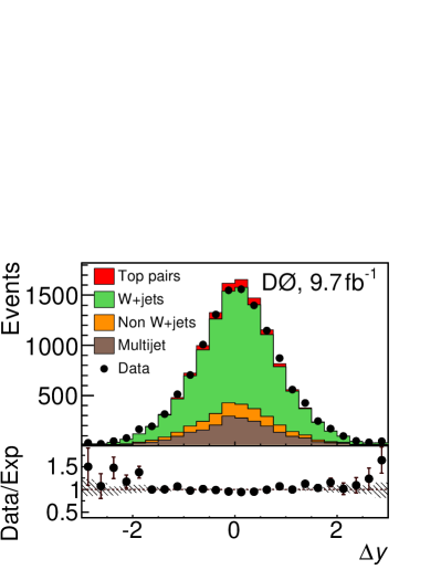
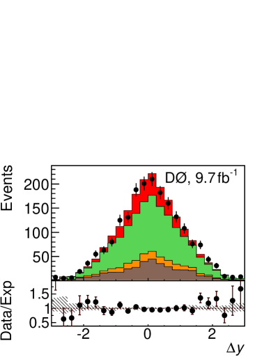
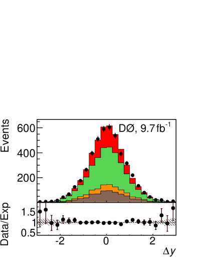
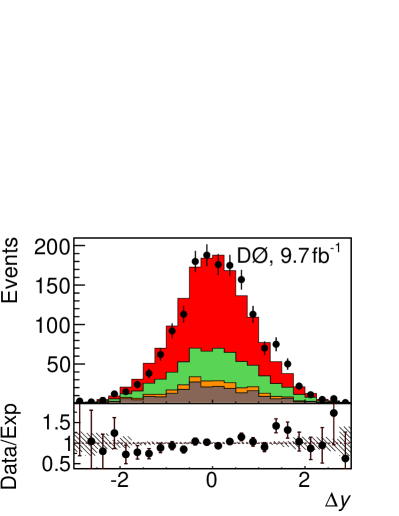
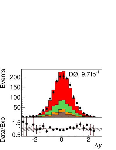
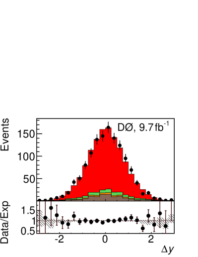
The distributions of the reconstructed are shown in Fig. 3. The asymmetry at the reconstruction level is extracted using a fit to the distributions in the discriminant and sign of , excluding the events with zero tags. This fitting procedure is identical to the procedure used in Ref. bib:our_afbl . The inclusive asymmetry measured at the reconstruction level is . The results for individual channels are listed in Table 3.
| , % | ||
|---|---|---|
| Channel | Predicted | Measured |
| 3 jets, tag | ||
| 3 jets, 2 tags | ||
| 4 jets, tag | ||
| 4 jets, 2 tags | ||
| Combined | ||
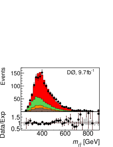
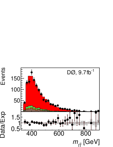
The distributions of the reconstructed invariant mass of the system are shown in Fig. 4. Since the and +4 jet channels have different response (both mean and shape) for , the dependence of on at the reconstruction level is difficult to interpret and is not presented here. The measurement of production/level and its dependence on is described in Section VII.
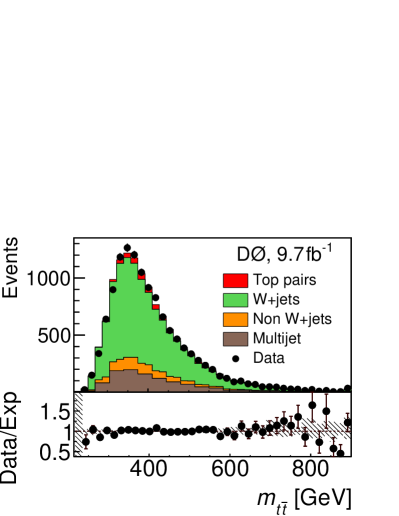
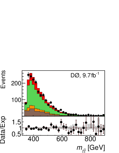
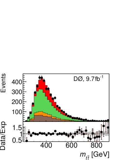
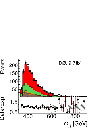
We use the results of the sample composition study summarized in Table 2 to normalize the distributions for the background processes in the sensitive variables (, and also for the 2D measurement), which are subtracted from the distributions observed in data. To increase the signal purity of the data used in the fully corrected measurements, we unfold only events containing at least one tag. The background/subtracted distributions of the sensitive variables in the corresponding four channels are used as inputs to the unfolding procedure.
VII Unfolding the asymmetry
The true or generated distribution of a certain variable ( for the inclusive measurement) is shaped by acceptance and detector resolution, resulting in the observed distribution, which is also subject to statistical fluctuations. The goal of the unfolding procedure is to find the best estimator for the true distribution given the background-subtracted data and knowing detector acceptance and resolution from simulation. After finding the best estimator for the true distribution of , we summarize it into the production/level using Eq. 2. This is the same general approach used in the previous measurement bib:ourPRD . For this unfolding we use TUNFOLD bib:tunfold , which we extend as discussed below.
Each distribution is presented as event counts in a binned histogram555Overflows are included in the edge bins., i.e., as a vector with a dimension equal to the number of bins. Given the vector of production/level signal counts, , and the vector of expected background counts, , the expected data counts in the -th bin is given by
| (4) | |||
| (5) |
where is a diagonal acceptance matrix, whose element is the probability for an event produced in the -th bin to pass the selection criteria and is the normalized migration matrix, whose element is the probability for a selected event produced in the -th bin to be observed in the -th bin.
Given the vector of observed counts, , we can construct the vector of background/subtracted reconstruction/level counts, , with its covariance error matrix . The matrix is constructed to account for the expected statistical uncertainties on data and background, in particular those due to the size of the multijet-enriched control sample. We then seek to find the vector , which best estimates the vector of production/level counts , by minimizing
| (6) |
for a given vector , where is the regularization strength and is the regularization matrix. The first term of Eq. 6 quantifies the consistency of with data, while the second (regularization) term quantifies the smoothness of .
Without regularization, the unfolding procedure amounts to a minimization of the first term in Eq. 6. If the numbers of reconstruction and production/level bins are equal, the problem of minimization is solved by simply inverting the matrix: .
Unregularized matrix inversion typically results in unphysical, rapidly varying distributions bib:zechbook . Such distributions are disfavored in regularized unfolding by adding a second “regularization” term to the . The regularization term in Eq. 6 depends on the discrete second derivative of the binned distribution . For constant bin widths, the regularization term is calculated using a regularization matrix with the following structure bib:tunfold :
| (7) |
For this analysis we modify the structure of to regularize based on the second derivative of the event density rather than the event counts, which allows for the use of variable bin sizes. The regularization strength is chosen using both ensemble testing (described below) and the L-curve technique bib:tunfold to balance the minimization of statistical fluctuations and bias. The difference between the two techniques is included in the evaluation of the systematic uncertainty due to the choice of the regularization strength.
As in Ref. bib:ourPRD , the production/level distribution is divided into 26 bins and the reconstruction/level distribution is divided into 50 bins. Both have narrower bins near , where the probability to misclassify forward events as backward or vice versa changes rapidly, and wider bins at high , where statistics are low.
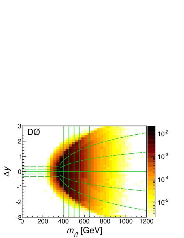
For the 2D measurement, we use six bins at the production level, with edges at 0, 400, 450, 500, 550, 650 GeV and . The joint distribution of and has a kinematic boundary at , where . A bin edge close to this boundary would result in a large difference in the event density between adjacent bins, a feature that would be smoothed by a regularization procedure, thus biasing . To avoid such a bias, the edges of the bins of the 2D measurement are chosen to depend on as shown in Fig 5.
The reconstruction/level histograms have similar but finer bins along both the and directions. In the channels 13 bins are used to accurately describe migrations among the six production/level bins. The resolution in the +4 jet channels allows for 14 bins.
We simultaneously unfold to the production level the four channels that contain at least one tag. The difference in purity among channels is accounted for in the definition of the covariance error matrix . The unfolding technique is calibrated, and the statistical and systematical uncertainties are determined using the results of ensemble tests. Each ensemble comprises simulated PDs that we build according to MC@NLO, ALPGEN bib:alpgen or MADGRAPH bib:madgraph SM predictions, or according to toy models with different asymmetries. The PDs are created from the expected bin counts calculated using Eq. 4 by adding Poisson (statistical) and Gaussian (systematic) fluctuations, with the Gaussian width taken as one standard deviation for the corresponding systematic uncertainty.
In the toy models the input distribution has the form:
| (8) |
where and are shaping parameters, is a Gaussian distribution with mean and width , the width predicted by MC@NLO, and a scaling parameter. The shape of the distribution and the input asymmetry are varied using the parameters , , , and . In addition, we produce ensembles with the signal taken from simulated samples of production mediated by axigluons, hypothetical massive particles that arise in extensions of the SM that suggest different strong couplings for left and right-handed quarks bib:axigluon . The input asymmetry in the models used for calibration ranges from to , while the axigluon masses are varied from to .
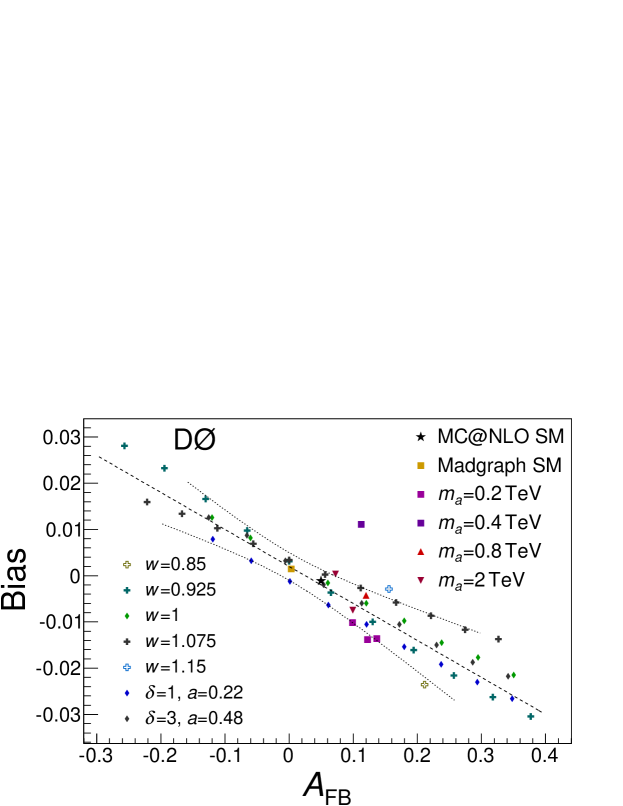
The bias, which is the average difference between the unfolded and input values, is shown in Fig. 6 as a function of the input . Based on this study we derive a correction (calibration) that is applied to the result to eliminate the expected bias. The majority of the tested models are contained within the systematic uncertainty assigned to this calibration, which is shown by the dotted lines in Fig. 6. The one point that is significantly outside of the boundaries of this region corresponds to production mediated by an axigluon with a mass of . This particular model exhibits a significant change in on the scale smaller than the bin width (here, 50 GeV), thus breaking the assumption of a smooth underlying distribution, leading to biased results. The unfolding of models with such rapidly changing will, in general, be biased in all regularized unfolding procedures, and we choose not to assign a systematic uncertainty that covers this specific class of models.
The unfolded distribution is presented in eight bins, with each bin calibrated for the expected bias observed in the MC@NLO/simulated PDs. The value in each range, , is calibrated using the same procedure as for the inclusive . Since no systematic correlation is found between the biases in different , as well as bins, they are calibrated individually.
VIII Systematic uncertainties
The systematic uncertainties on the reconstruction and production/level are summarized in Table 4 in several categories, which are detailed below. To evaluate the systematic uncertainty on the reconstruction/level , we vary the modeling according to the estimated uncertainty in the relevant parameter of the model and propagate the effect to the result. The systematic uncertainties on the production/level are evaluated by including the effects of systematic variations on the simulated background-subtracted PD into the ensemble tests. To find the expected uncertainty due to each category we use dedicated ensembles generated without statistical fluctuations and with only the relevant systematic effects. The total uncertainties on the production/level are taken from ensembles built including both statistical fluctuations and systematic effects (see Sec. VII).
| Reco. level | Production level | ||
|---|---|---|---|
| Source | inclusive | inclusive | 2D |
| Background model | / | – | |
| Signal model | – | ||
| Unfolding | N/A | – | |
| PDFs and pileup | – | ||
| Detector model | / | – | |
| Sample composition | |||
| Total | / | – | |
The background model category includes the following sources, which affect the properties predicted for background events. The leptonic asymmetry of the jets background is varied within its uncertainty of bib:our_afbl . The rate of heavy-flavor production within jets production is varied by bib:D0xsect ; bib:mcfm . The efficiencies for lepton identification, and the probabilities for a jet to be misidentified as a lepton, taken as functions of lepton momentum, are varied within their uncertainties to account for the uncertainty on the number of background events from multijet production bib:matrix_method . This variation affects both the background shape and normalization. Uncertainties associated with the modeling of the discriminant, , transverse momentum of boson and , as well as potentially increased background levels at high lepton pseudorapidity are also quantified by modifying the background model bib:our_afbl .
The signal model category includes the sources of uncertainty that affect the properties predicted for signal events other than the ones accounted for in the PDFs and pileup category. The top quark mass is varied according to the combined Tevatron measurement of Ref. bib:mtop . The effect of higher order corrections to production is estimated by replacing the migration matrix from Eq. 4 simulated by MC@NLO with the one simulated by ALPGEN, which uses tree-level matrix elements. The quark fragmentation function is varied within its uncertainties bib:mtop , which also affects background modeling.
The signal model category also includes the uncertainties associated with gluon radiation. The total amount of initial state radiation is varied in a range consistent with the results of Ref. bib:Zisr . We also consider the difference in the predicted amount of initial state radiation between forward and backward events, both because of contributions at order and due to higher order effects which are modeled by the simulated parton showers bib:winter . We account for this uncertainty by reducing the difference in the distributions of the of the system for forward and backward events by 25%, a value derived from Ref. bib:winter . We also account for the possibility that the mismodeling of this variable in the final state affects by reweighting this distribution to match the D0 data, similarly to the procedure used in Ref. bib:our_afbl .
The uncertainties due to unfolding are dominated by the calibration uncertainties. The uncertainties associated with the choice of the regularization strength and statistical fluctuations in the MC samples used to find the migration matrix are also included.
The PDFs and pileup category includes uncertainties on the modeling of the collisions. The main uncertainties are from the PDFs, which primarily affect the distribution of the jets background. These uncertainties are evaluated by varying the contributions of the various eigenvectors from the CTEQ6.1 PDF bib:CTEQ and by considering an alternative set of PDFs (MRST2003 bib:MRST ). The number of additional collisions within the same bunch crossing (pileup) affects the quality of the reconstruction. The uncertainties on the modeling of additional collisions are also included in this category.
The detector model category includes the following sources of systematic uncertainty. The efficiencies of the -tagging algorithm for jets of different flavors, which are measured from collider data, are varied according to their uncertainties bib:btagging . These variations affect the measured mostly through the estimated sample composition, which depends strongly on the classification of data into several channels according to the number of tags. The modeling of jet energy reconstruction, including the overall energy scale and the energy resolution, as well as jet-reconstruction efficiencies and single-particle responses, are all calibrated to collider data and are varied according to their uncertainties bib:Jets . The uncertainties due to jet reconstruction and energy measurement are significantly reduced compared to the previous measurement due to the inclusion of the events.
Lastly, the sample composition is varied according to its fitted uncertainties. This variation is performed in addition to the changes in the sample composition implicitly induced by other systematic variations.
IX Results
IX.1 Inclusive and dependence on
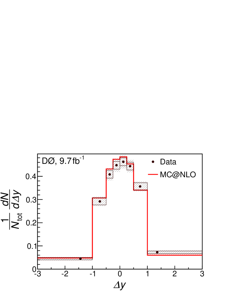
The calibrated production/level distribution is shown in Fig. 7. The corresponding inclusive forward–backward asymmetry in production is .
| ,% | ||
| Predicted | Measured | |
| 1.1 | ||
| 0.25–0.5 | 2.5 | |
| 0.5–1 | 5.2 | |
| 11.4 | ||
| range | ||||
|---|---|---|---|---|
| 0.25–0.5 | 0.5–1 | |||
| 0.25–0.5 | ||||
| 0.5–1 | ||||
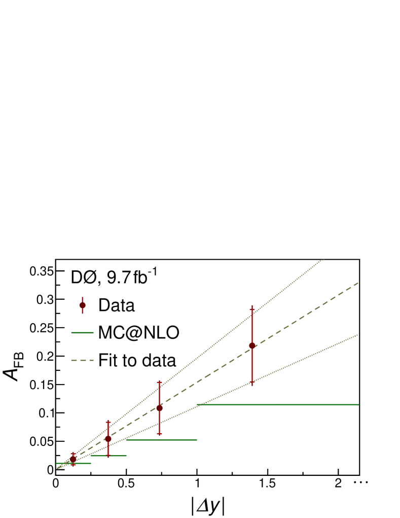
The dependence of on is shown in Fig. 8 and Table 5 with the correlation factors between bins listed in Table 6. These correlations are taken into account in the fit of the measured to a line. Since for any physical distribution the asymmetry at is 0, we constrain the line to the origin and fit for its slope. For data, we find a slope of . This slope is compatible within two standard deviations with the MC@NLO-simulated slope of , which has negligible statistical uncertainty. The difference between the slope reported by the CDF Collaboration bib:CDF2012 and the slope reported in this paper corresponds to standard deviations666When comparing to CDF results, we neglect the correlations of the systematic uncertainties between the two experiments..
IX.2 dependence on
The dependence of on is shown in Fig. 9 and Table 7 with the correlation factors between bins listed in Table 8.
| ,% | ||
| , GeV | Predicted | Measured |
| – | ||
| – | ||
| – | ||
| – | ||
| Inclusive | ||
| range ( GeV) | ||||||
|---|---|---|---|---|---|---|
| – | – | – | – | |||
| – | ||||||
| – | ||||||
| – | ||||||
| – | ||||||
| Eigenvector | |||||||
|---|---|---|---|---|---|---|---|
| Parameter | Predicted | Measured |
|---|---|---|
| Slope, | ||
| Offset, |
The values of the asymmetry measured in six ranges constitute a six-dimensional vector with a covariance matrix . Table 9 lists the eigenvectors of together with the corresponding components of the vector in the basis formed by the eigenvectors: , and their uncertainties , where is the covariance matrix transformed to the basis . The elements of Table 9 fully specify the measured six-dimensional likelihood in the Gaussian approximation, and can be used for quantitative comparison with theoretical predictions and other experimental results bib:zech_proc .
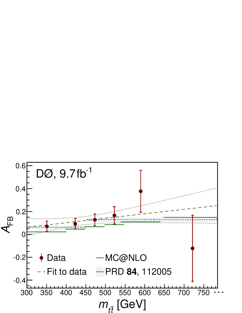
Using the full covariance matrix we perform a fit of the measured to the functional form
| (9) |
We choose so that the correlation factor between the fit parameters and is less than in the fit to the data. The parameters of the fit are listed in Table 10 for the data and the MC@NLO simulation. We observe a slope consistent with zero and with the MC@NLO prediction. The difference between slope reported by the CDF Collaboration bib:CDF2012 and the slope reported in this paper corresponds to standard deviations.
X Discussion
The measured inclusive forward–backward asymmetry in production, is in agreement with the SM predictions reviewed in Section V, which range from an inclusive asymmetry of 5.0% predicted by the MC@NLO simulation to % bib:EWcorr once electroweak effects are taken into account. The measured dependences of the asymmetry on and are also in agreement with the SM predictions. Nevertheless, the observed and the dependences of on and do not disfavor the larger asymmetries that were previously measured in collisions bib:CDF2012 .
To compare the presented result with the previous D0 publication bib:ourPRD , Table 11 presents at the reconstruction level measured in different samples. The method discussed in this paper applied to +4 jet events from the first 5.4 of integrated luminosity yields a result consistent with that in Ref. bib:ourPRD , but with a reduced uncertainty mainly due to the separation of data into channels based on the number of tags and the increased efficiency of the new -tagging algorithm. Once the analysis is extended to include the events collected at that time, the uncertainty is reduced by a factor of 1.26. The result obtained in the second 4.3 of the Tevatron dataset is within one standard deviation from that obtained in the first 5.4. The statistical uncertainty obtained in the combined 9.7 of integrated luminosity is reduced by a factor of 1.29 with respect to the result obtained using the same method in the first 5.4, while the reduction expected from scaling with the integrated luminosity is 1.34. This loss of sensitivity is mainly due to higher instantaneous luminosity during the collection of the later data, which required a tighter trigger selection.
| Reco-level | ||
|---|---|---|
| Sample | Method | , % |
| +4 jet, first 5.4 | From Ref. bib:ourPRD | |
| +4 jet, first 5.4 | This analysis | |
| +3 jet, first 5.4 | This analysis | |
| +3 jet, additional 4.3 | This analysis | |
| +3 jet, full 9.7 | This analysis |
The improved reconstruction of and the reduced acceptance bias due to the inclusion of the events result in further reduction of the statistical uncertainty on the unfolded result compared to Ref. bib:ourPRD . The separation of the data into channels allows us to add the channels without losing the statistical power of the purer +4 jet channels.
XI Summary
In summary, we report the measurement of the forward–backward asymmetry in production using the dataset recorded by the D0 detector in Run II of the Fermilab Tevatron Collider. The results presented here supersede the ones that were based on about half of the data bib:ourPRD . The analysis is extended to include events with three jets, allowing for the loss of one jet from the decay and reducing the acceptance corrections. The unfolding procedure now accounts for the differences in sample compositions between channels, thus maximizing the statistical strength of the individual channels. New reconstruction techniques are used in the +4 jet channel, improving the experimental resolution in all variables of interest.
The asymmetry measured at the reconstruction level is . After correcting for detector resolution and acceptance, we obtain a production/level asymmetry . The observed asymmetry and the dependences of on and are consistent with the standard model predictions.
Acknowledgements.
We thank M. Mangano, P. Skands and G. Perez for enlightening discussions. We thank the staffs at Fermilab and collaborating institutions, and acknowledge support from the DOE and NSF (USA); CEA and CNRS/IN2P3 (France); MON, NRC KI and RFBR (Russia); CNPq, FAPERJ, FAPESP and FUNDUNESP (Brazil); DAE and DST (India); Colciencias (Colombia); CONACyT (Mexico); NRF (Korea); FOM (The Netherlands); STFC and the Royal Society (United Kingdom); MSMT and GACR (Czech Republic); BMBF and DFG (Germany); SFI (Ireland); The Swedish Research Council (Sweden); and CAS and CNSF (China).References
- (1) V. M. Abazov et al. (D0 Collaboration), Phys. Rev. Lett. 100, 142002 (2008).
- (2) T. Aaltonen et al. (CDF Collaboration), Phys. Rev. Lett. 101, 202001 (2008).
- (3) T. Aaltonen et al. (CDF Collaboration), Phys. Rev. D 83, 112003 (2011).
- (4) V. Abazov et al. (D0 Collaboration), Phys. Rev. D 84, 112005 (2011).
- (5) T. Aaltonen et al. (CDF Collaboration), Phys. Rev. D 87, 092002 (2013).
- (6) J. H. Kühn and G. Rodrigo, Phys. Rev. Lett. 81, 49 (1998).
-
(7)
L. G. Almeida, G. Sterman, and W. Vogelsang,
Phys. Rev. D 78, 014008 (2008);
M. T. Bowen, S. D. Ellis, and D. Rainwater, Phys. Rev. D 73, 014008 (2006);
S. Dittmaier, P. Uwer, and S. Weinzierl, Phys. Rev. Lett. 98, 262002 (2007);
K. Melnikov and M. Schulze, Nucl. Phys. B 840, 129 (2010);
J. H. Kühn and G. Rodrigo, J. High Energy Phys. 01 (2012) 063. -
(8)
For a review: J. F. Kamenik, J. Shu and J. Zupan,
Eur. Phys. J. C 72, 2102 (2012);
See also Refs. 3–83 of E. L. Berger, Q.-H. Cao, C.-R. Chen and H. Zhang, Phys. Rev. D 88, 014033 (2013). - (9) P. H. Frampton and S. L. Glashow, Phys. Lett. B 190, 157 (1987).
- (10) V. M. Abazov et al. (D0 Collaboration), submitted to Phys. Rev. D, arXiv:1403.1294 [hep-ex].
- (11) V. M. Abazov et al. (D0 Collaboration), submitted to Nucl. Instrum. Methods A, arXiv:1312.7623 [hep-ex]. In this paper, jets with are tagged.
-
(12)
V. M. Abazov et al. (D0 Collaboration),
Nucl. Instrum. Meth. A 565, 463 (2006);
R. Angstadt et al. (D0 Collaboration), Nucl. Instrum. Meth. A 622, 298 (2010). - (13) V. M. Abazov et al. [D0 Collaboration], submitted to Nucl. Instrum. Meth. A, arXiv:1401.0029 [hep-ex].
- (14) S. Abachi et al. (D0 Collaboration), Nucl. Instrum. Meth. A 338, 185 (1994).
- (15) V. M. Abazov et al. (D0 Collaboration), Nucl. Instrum. Meth. A 552, 372 (2005).
- (16) V. M. Abazov et al. [D0 Collaboration], Nucl. Instrum. Meth. A 737, 281 (2014).
- (17) M. Abolins et al., Nucl. Instrum. Meth. A 584, 75 (2008).
-
(18)
S. Frixione and B. R. Webber,
J. High Energy Phys. 06 (2002) 029;
S. Frixione, P. Nason and B. R. Webber, J. High Energy Phys. 08 (2003) 007. - (19) G. Corcella et al., J. High Energy Phys. 01 (2001) 010.
- (20) M. L. Mangano et al., hep-ph/0206293, CERN-TH-2002-129 (2002).
- (21) T. Sjöstrand et al., Comput. Phys. Commun. 135, 238 (2001).
- (22) D. Stump et al., J. High Energy Phys. 10 (2003) 046.
- (23) V. M. Abazov et al. (D0 Collaboration), Phys. Rev. D 84, 012008 (2011).
- (24) E. Boos et al. (CompHEP Collaboration), Nucl. Instrum. Meth. A 534, 250 (2004).
- (25) J. M. Campbell and R. K. Ellis, Nucl. Phys. Proc. Suppl. 205, 10 (2010).
- (26) R. Brun and F. Carminati, CERN Program Library Long Writeup W5013 (1993) (unpublished).
- (27) S. Snyder, “Measurement of the Top Quark mass at D0”, Doctoral Thesis, State University of New York at Stony Brook (1995).
- (28) B. A. Betchart, R. Demina, and A. Harel, Nucl. Instrum. Meth. A 736, 169 (2014).
- (29) I. Volobouev, arXiv:1101.2259 [physics.data-an].
- (30) R. Demina, A. Harel, and D. Orbaker, arXiv:1310.3263 [hep-ex].
- (31) V. Abazov et al. (D0 Collaboration), Phys. Rev. D 85, 051101 (2012).
- (32) A. Hoecker, P. Speckmayer, J. Stelzer, J. Therhaag, E. von Toerne, and H. Voss, “TMVA: Toolkit for Multivariate Data Analysis,” PoS A CAT 040 (2007) [physics/0703039].
- (33) Private communications with W. Bernreuther, updating the error estimates of Ref. bib:EWcorr .
- (34) M. Czakon, P. Fiedler, and A. Mitov, Phys. Rev. Lett. 110, 252004 (2011).
- (35) W. Bernreuther and Z.-G. Si, Phys. Rev. D 86, 034026 (2012), and references therein.
-
(36)
e.g., L. G. Almeida, G. F. Sterman and W. Vogelsang,
Phys. Rev. D 78, 014008 (2008);
N. Kidonakis, Phys. Rev. D 84, 011504 (2011). - (37) J. M. Campbell and R. K. Ellis, arXiv:1204.1513 [hep-ph].
-
(38)
S. J. Brodsky and X.-G. Wu,
Phys. Rev. D 85, 114040 (2012);
X.-G. Wu, S. J. Brodsky, and M. Mojaza, Prog. Part. Nucl. Phys. 72, 44 (2013);
S. J. Brodsky, M. Mojaza and X.-G. Wu, Phys. Rev. D 89, 014027 (2014). - (39) S. J. Brodsky, Annu. Rev. Nucl. Part. Sci. 2012.62, 1 (2012).
- (40) G. Hanson et al., Phys. Rev. Lett. 35, 1609 (1975).
- (41) F. Abe et al. (CDF Collaboration), Phys. Rev. Lett. 81, 5754 (1998).
-
(42)
http://root.cern.ch/root/html/TUnfold.html and reference within.
In particular: http://www.desy.de/~sschmitt and
P. C. Hansen, in Computational Inverse Problems in Electrocardiology, ed. P. Johnston, Advances in Computational Bioengineering (2000),
http://www.imm.dtu.dk/~pch/TR/Lcurve.ps -
(43)
G. Bohm and G. Zech, “Introduction to Statistics and Data Analysis for Physicists”,
Verlag Deutsches Elektronen-Synchrotron,
http://www-library.desy.de/elbook.html (2010). - (44) J. Alwall et al., J. High Energy Phys. 06 (2011) 128.
- (45) V. M. Abazov et al. (D0 Collaboration), Phys. Rev. D 84, 012008 (2011).
- (46) T. Aaltonen et al. (CDF and D0 Collaborations), Phys. Rev. D 86, 092003 (2012).
- (47) V. M. Abazov et al. (D0 Collaboration), Phys. Rev. Lett. 106, 122001 (2011).
-
(48)
P. Skands, B. Webber, and J. Winter,
J. High Energy Phys. 07 (2012) 151;
J. Winter, P. Z. Skands, and B. R. Webber, Eur. Phys. J. C 49, 17001 (2013). - (49) A. D. Martin, R. G. Roberts, W. J. Stirling, and R. S. Thorne, Eur. Phys. J. C 35, 325 (2004).
- (50) V. M. Abazov et al. (D0 Collaboration), submitted to Nucl. Instrum. Meth. A, arXiv:1312.6873 [hep-ex].
- (51) G. Zech, in Proceedings of the PHYSTAT 2011 Workshop on Statistical Issues Related to Discovery Claims in Search Experiments and Unfolding, 10.5170/CERN-2011-006 (2011).