Atomic carbon as a powerful tracer of molecular gas in the high-redshift Universe: perspectives for ALMA

Abstract

We use a high-resolution hydrodynamic simulation that tracks the non-equilibrium abundance of molecular hydrogen within a massive high-redshift galaxy to produce mock Atacama Large Millimeter Array (ALMA) maps of the fine-structure lines of atomic carbon, Ci 1-0 and Ci 2-1. Inspired by recent observational and theoretical work, we assume that Ci is thoroughly mixed within giant molecular clouds and demonstrate that its emission is an excellent proxy for H₂. Nearly all of the H₂ associated with the galaxy can be detected at redshifts $z<4$ using a compact interferometric configuration with a large synthesized beam (that does not resolve the target galaxy) in less than 4 h of integration time. Low-resolution imaging of the Ci lines (in which the target galaxy is resolved into three to four beams) will detect $\sim$80 per cent of the H₂ in less than 12 h of aperture synthesis. In this case, the resulting data cube also provides the crucial information necessary for determining the dynamical state of the galaxy. We conclude that ALMA observations of the Ci 1-0 and 2-1 emission are well-suited for extending the interval of cosmic look-back time over which the H₂ distributions, the dynamical masses, and the Tully-Fisher relation of galaxies can be robustly probed.

1 Introduction

Forbidden fine-structure lines of neutral atomic carbon can be used as tracers of the molecular mass in galaxies (Gerin & Phillips, 2000; Papadopoulos et al., 2004). The ground electronic state of neutral carbon, $\rm 1s^{2}\,2s^{2}\,2p^{2}$, is split into five fine-structure levels that, in spectroscopic notation, are denoted by $\rm{}^{3}P_{J}$ (with $J=0,1$ and 2), $\rm{}^{1}D_{2}$, and $\rm{}^{1}S_{0}$. The excited fine levels $\rm{}^{3}P_{1}$ and $\rm{}^{3}P_{2}$ lie only 23.6 and 62.4 K above the ground state ($\rm{}^{3}P_{0}$) and are therefore easily populated by particle collisions in the cold interstellar medium. Two magnetic-dipole transitions are allowed between the fine-structure levels: $\rm{}^{3}P_{1}\to{\rm{}^{3}P_{0}}$ (which we refer to as Ci 1–0) has a rest frequency of 492.1607 GHz, while $\rm{}^{3}P_{2}\to{\rm{}^{3}P_{1}}$ (Ci 2–1) produces electromagnetic radiation at 809.3435 GHz.

Early one-dimensional models of photon-dominated regions (PDRs) confined the presence of Ci to a thin transition layer separating the outer ionized zone from the CO-rich inner volume (Kaufman et al., 1999). However, large-scale Ci surveys of the Orion A and B molecular clouds (Ikeda et al., 2002) and of the Galactic center (Ojha et al., 2001) as well as observations of nearby galaxies (Israel & Baas, 2002; Zhang et al., 2014) have found that the Ci 1–0, 2–1 line emission is fully concomitant and strongly correlates with ${}^{12}\rm CO$ intensity. In addition, several observations (e.g. Frerking et al., 1989; Schilke et al., 1995; Kramer et al., 2008) have shown that Ci is ubiquitous in giant molecular clouds (GMCs). Clumpy PDR models (e.g. Spaans, 1996) suggest that the surface layers of Ci are evenly spread across GMCs. Moreover turbulent diffusion, cosmic ray fluxes, and non-equilibrium chemistry all help to maintain a nearly constant $[\textsc{Ci}~{}\!\!]/[\rm H_{2}]$ abundance ratio throughout most of the mass of a typical molecular cloud (Papadopoulos et al., 2004). A recent numerical simulation of a turbulent molecular cloud confirms that Ci emission should be widespread in GMCs, with most of the neutral carbon at gas densities between $10^{2}$ and $10^{4}$ cm^-3 and kinetic temperatures of $T_{\rm k}\sim$ 30 K (Glover et al., 2014).

Sensitivity limitations and the low atmospheric trasmissivity in the short sub-mm regime made the detection and imaging of Ci lines in the local Universe difficult (hampering the realization that they do not conform to the standard stratified PDR picture). At redshifts $z\sim 2-4$, where the Ci lines are redshifted into more favourable atmospheric windows, only a handful of galaxies have been observed in the 1–0 and 2–1 transitions (Weiß et al., 2003, 2005; Walter et al., 2011; Alaghband-Zadeh et al., 2013, and references therein). However, this sample will undoubtedly grow in size due to forthcoming observations from the Plateau de Bure Interferometer (possibly upgraded to the Northern Extended Millimeter Array), the Submillimeter Array, the Atacama Pathfinder Experiment and the Atacama Large Millimeter Array (ALMA), as well as with the advent of new facilities such as and the Cerro Chajnantor Atacama Telescope. The improved sensitivity of these instruments will yield observations that significantly enhance our understanding of the molecular gas content of distant galaxies and of the history of cosmic star formation.

In this letter, we use a fully cosmological simulation of the formation of a massive, high-redshift galaxy and track its non-equilibrium H₂ abundance across cosmic time. Using this simulation, we produce mock ALMA maps of the associated Ci 1-0 and Ci 2-1 fine-structure line emission, and demonstrate that such observations can be used to robustly estimate the molecular content of massive systems at high redshifts.

2 Methods

The simulation follows the formation of a massive galaxy up to $z=2$ in its full cosmological context using the adaptive-mesh-refinement code ramses (Teyssier, 2002). It achieves a physical resolution $\simeq\,180$ pc, and includes gas cooling, star formation, feedback and metal enrichment from stellar evolution. We use a novel sub-grid treatment of the formation and destruction of molecular hydrogen within unresolved GMCs to track the non-equilibrium abundance of H₂. At $z=2$, the galaxy has a stellar mass of $7.7\times 10^{10}$ M_⊙, a star-formation rate of 43 M_⊙ yr^-1 and an H₂ mass of $4.4\times 10^{10}$ M_⊙, which are consistent with the properties of sub-mm galaxies for which Ci emission has been already detected at $z>2$. This simulation is described in full detail in Tomassetti et al. (2014), to which we refer the reader for further details.

To produce Ci 1-0 and Ci 2-1 emission maps, we assume that atomic carbon is thoroughly mixed with molecular hydrogen and that the $[\textsc{Ci}~{}\!\!]/[\rm H_{2}]$ abundance ratio is constant on kpc scales. (This quantity is observed to range between $10^{-5}$ and $10^{-4}$ in non-star-forming and star-forming clouds, respectively (Frerking et al., 1989; Weiß et al., 2005; Walter et al., 2011; Danielson et al., 2011)). In the following, we adopt the representative value of $[\textsc{Ci}~{}\!\!]/[\rm H_{2}]\simeq 3\times 10^{-5}$ (Alaghband-Zadeh et al., 2013), but discuss in Section 3 how changes to this parameter affect our results.

At the frequencies of the Ci fine-structure lines our simulated galaxy is optically thin and the flux density per unit frequency observed on Earth, $S_{\textsc{Ci}~{}\!\!}$, for the transition between levels u and l is

$$S_{\textsc{Ci}~{}\!\!}=\frac{A_{\rm ul}\,h\nu_{\rm ul}\,\Omega_{\rm B}\,Q_{\rm u}\overline{N}_{\textsc{Ci}~{}\!\!,\Delta\nu}}{4{\rm\pi}\,(1+z)^{4}\Delta\nu}.$$ (1)

Here $A_{\rm ul}$ is the Einstein coefficient, $h$ is the Planck constant, $\nu_{\rm ul}$ the rest-frequency of the transition, $\Omega_{\rm B}$ the beam size, $z$ the redshift at which the galaxy is observed and $\Delta\nu$ the frequency bandwidth. The term $\overline{N}_{\textsc{Ci}~{}\!\!,\Delta\nu}$ denotes the beam-averaged column density of carbon atoms with line-of-sight velocities corresponding to the frequency range $\Delta\nu$ for the line transition. Lastly, $Q_{\rm u}=n_{\rm u}/n_{\textsc{Ci}~{}\!\!}<1$ is the fractional population of level u, where $n_{\textsc{Ci}~{}\!\!}$ is the total number density of atomic carbon. Given that the critical densities of the Ci transitions are comparable to the densities of GMCs, it is reasonable to compute $Q_{\rm u}$ assuming local thermodynamic equilibrium (LTE). We assume a gas kinetic temperature of $T_{\rm k}=30$ K (Walter et al., 2011), for which $Q_{\rm 1}\simeq 0.46$ and $Q_{\rm 2}\simeq 0.21$. The impact of varying $T_{\rm k}$ is discussed in the next section.

Our goal is to demonstrate the power of using Ci ​​-line ALMA observations to estimate the H₂ mass of high-$z$ galaxies. Noise levels are computed using the ALMA sensitivity calculator for an array configuration of fifty 12 m antennas. We assume that our simulated galaxy is observed at an elevation of 45^∘ and adopt a water vapour column density of $1.8$ mm.

3 Results

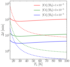
Figure 1: Integration time, $\Delta t$, required to detect the Ci signal from our simulated galaxy at $z=2$ as a function of the kinetic gas temperature. We plot the time required to observe the brightest pixel with a signal-to-noise ratio of five in the (continuum-subtracted) surface-brightness maps. All curves refer to a compact ALMA configuration with a baseline length of $D=150$ m whose synthesized beam is larger than the simulated galaxy at the observed redshift. We assume that our galaxy is observed at an elevation of 45^∘. Solid and dashed lines refer to the 1-0 and 2-1 transitions, respectively.

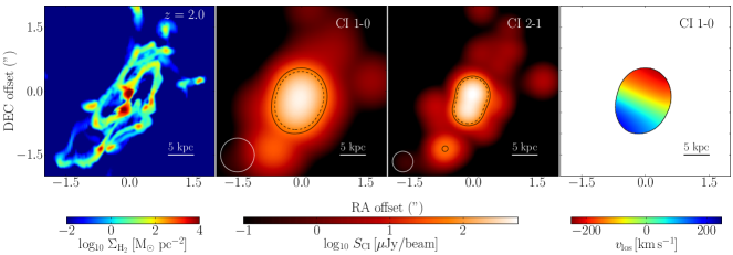
Figure 2: Left: simulated H₂ surface density at $z=2$. Middle: flux density of the Ci 1–0 (middle-left) and 2–1 (middle-right) transitions for the projection shown on the left assuming a bandwidth $\Delta v=\pm 2\sigma$ and a baseline $D=700$ m. Contours are drawn at S/N levels of 3 (solid) and 5 (dashed) for an integration time of $\Delta t=12$ h; white circles in the lower-left corners indicate the beam shape and size. Right: flux-weighted mean velocity map determined from the Ci 1-0 signal using velocity channels of 50 km s^-1. Contours show S/N=3 for $\Delta t=12$ h for the flux density in the middle-left panel. Mock observations assume that our galaxy is observed at an elevation of 45^∘.

For a detection experiment, we first consider a compact ALMA configuration with a baseline length of $D=150$ m. In this case, the synthesized beam is large (for observations at $z=2$, it has an FWHM of $3.1$ and $1.9$ arcsec for Ci 1–0 and 2–1, respectively) and the simulated galaxy is not spatially resolved at any redshift $z>2$. In Fig. 1 we show, as a function of $T_{\rm k}$, the integration time required to detect the galaxy at $z=2$. We integrate the data cube over the velocity range $\Delta v\simeq\pm 450$ km s^-1, which corresponds to four times the line-of-sight velocity dispersion, $\sigma$, of the H₂ gas within the beam. We compute the integration time by requiring the brightest pixel in the (continuum subtracted) surface-brightness map to have a signal-to-noise (S/N) ratio of 5. For our fiducial values of the kinetic temperature and carbon abundance, approximately 4 min of exposure is enough to detect the 2–1 line, whereas 8 min are needed for the 1–0 line. These values scale as $([\textsc{Ci}~{}\!\!]/[\rm H_{2}])^{-2}\,Q_{\rm u}^{-2}$, suggesting that 76 (34) min of integration is necessary for an abundance ratio of $\sim 10^{-5}$ for the 1–0 (2–1) line. Note that for high values of the gas temperature, the 2–1 line is brighter than the 1–0 line. However, it may be difficult to detect for $T_{\rm k}\ll 30$ K as the $\rm{}^{3}P_{2}$ level may not be significantly populated.

Using equation (1), we can estimate the H₂ mass contained within $\Omega_{\rm B}$, from the flux in the brightest pixel:

$$M_{\rm H_{2}}^{\rm max}=\frac{4{\rm\pi}\,m_{\textsc{Ci}~{}\!\!}\Delta v\,S_{\textsc{Ci}~{}\!\!}^{\rm max}\,D_{\rm L}^{2}}{6\,[\textsc{Ci}~{}\!\!]/[{\rm H_{2}}]\,A_{\rm ul}\,Q_{\rm u}\,h\,c\,(1+z)}.$$ (2)

Here $S_{\textsc{Ci}~{}\!\!}^{\rm max}$ is the pixel brightness, $m_{\textsc{Ci}~{}\!\!}$ is the mass of a carbon atom, $D_{\rm L}$ the luminosity distance and $c$ is the speed of light. For our assumed values of the Ci temperature and the $[\textsc{Ci}~{}\!\!]/[\rm H_{2}]$ abundance ratio, this gives $4.3\times 10^{10}$ M_⊙ and $4.0\times 10^{10}$ M_⊙ for the 1–0 and 2–1 transitions, respectively.

In practice the kinetic temperature can be determined using the line-intensity ratio Ci 2–1/Ci 1–0 under the assumption of LTE (e.g. Stutzki et al., 1997). One can use also the non-LTE $Q_{\rm u}(n,T_{\rm k}$) expressions (Papadopoulos et al. 2004), given certain constraints on the average gas density exist (e.g. via multi-$J$ CO and HCN line observations). However, the relative Ci abundance must be calibrated against multiple observations of other emission lines as well as measures of the dynamical mass in GMCs (e.g. from CO). Observational noise together with uncertainties in $T_{\rm k}$ and $[\textsc{Ci}~{}\!\!]/[\rm H_{2}]$ will, of course, generate scatter around our ideal results.

The spectrum extracted from the data cube at the location of the brightest pixel can be used to obtain $\sigma$ and the dynamical mass of the galaxy. Over the redshift range $2<z<3$, we find that dynamical masses, estimated as $M_{\rm dyn}=\alpha\,\sigma^{2}\,R_{\rm B}/G$ (where $G$ is the gravitational constant, $R_{\rm B}=\rm FWHM/(2\,\sqrt{\ln 2})$ the beam radius, and $\alpha=3.4$; Erb et al. 2006), are within a factor of two of the total mass within a spherical aperture of radius $R_{\rm B}$ centred on the galaxy.

Next, we construct low-resolution ALMA maps of the H₂ distribution within our simulated galaxy assuming a baseline length of $D=700$ m. At $z=2$, the galaxy is then resolved by three to four telescope beams (the FWHM of the ALMA beam is $0.7\,(5.6)$ and $0.4\,(3.4)$ arcsec (kpc) for the 1–0 and 2–1 transitions, respectively) and the noise level for an integration time $\Delta t$ and a velocity bandwidth of roughly $\pm 350$ km s^-1 is $\sigma_{\rm rms}\simeq 50\,(\Delta t/\rm 1\,h)^{-1/2}$ $\rm\mu$Jy beam^-1. The results are shown in Fig. 2. In the left-hand panel, we plot the H₂ surface density at the spatial resolution of the simulation (for a line of sight that forms an angle of 45^∘ with respect to the disk). The two middle panels show the corresponding Ci flux densities for the 1–0 (middle-left) and 2–1 (middle-right) transitions. Detecting the brightest pixel in the maps with an S/N ratio of 3 (5) requires an integration time of $\sim 7$ (20) min for the 1–0 transition and $\sim 5$ (14) min for 2–1. S/N contours drawn for an integration time of 12 h reveal that the detectable signal originates from regions where the beam-averaged H₂ column density is $\lower 3.01385pt\hbox{$\;\stackrel{{\scriptstyle\textstyle>}}{{\sim}}\;$}\,70$ M_⊙ pc^-2. In the right-hand panel, we use the data cube to draw a map of the mean line-of-sight velocity. Our results show that integration times on the order of 1 h are sufficient to retrieve detailed dynamical information.

It is useful to estimate how accurately we can reconstruct the H₂ mass of the galaxy from resolved imaging of the Ci 1–0 and 2–1 lines. To do so, we compute the H₂ mass that occupies the same volume as the observable carbon atoms. This is achieved by convolving the H₂ surface-density maps with the ALMA beam and integrating over the solid angle subtended by regions in which $S_{\textsc{Ci}~{}\!\!}$ is above a given flux limit, $S$. In Fig. 3, we show our results for the galaxy at $z=2$. The measured H₂ mass, $M_{\rm H_{2}}(>S)$, increases with decreasing the flux limit. For an integration time of 12 h, the H₂ mass recovered from the area over which $S_{\textsc{Ci}~{}\!\!}$ is above 3$\,\sigma_{\rm rms}$ is $3.6\times 10^{10}$ M_⊙ for the 1–0 line and $3.3\times 10^{10}$ M_⊙ for the 2–1 transition. Longer integrations, or reductions in the baseline length, boost the signal from low-density regions. For $D=400$ m, for example, one finds $4\times 10^{10}$ M_⊙ (for Ci 1–0) and $3.9\times 10^{10}$ M_⊙ (for Ci 2–1). These values can be directly compared to the H₂ mass of the galaxy: the grey shaded area in Fig. 3 shows the H₂ mass contained within 10 and 50 kpc from its center.

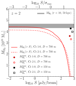
Figure 3: Red lines show the H₂ mass obtained by integrating over the solid angle subtended by regions over which $S_{\textsc{Ci}~{}\!\!}$ is above a given flux limit, $S$, for the 1–0 (solid line) and 2–1 (dashed line) transitions. The grey shaded region shows the H₂ mass that lies within $10$ and $50$ kpc from the centre of the galaxy at $z=2$. Symbols indicate the flux in the brightest pixel and the corresponding H₂ mass contained within $\Omega_{\rm B}$ as inferred from equation (2) for the 1–0 (filled symbols) and 2–1 (open symbols) transitions. Results are plotted for the $D=700$ m (circles) and $D=150$ m (squares) cases. The upper $x$-axis shows the corresponding S/N ratio for the 1–0 transition (and integration time $\Delta t=12$ h). For this plot we have adopted $[\textsc{Ci}~{}\!\!]/[\rm H_{2}]=3\times 10^{-5}$ and $T_{\rm k}=30$ K, and assumed an elevation of 45^∘.

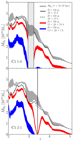
Figure 4: Molecular-hydrogen mass associated with our simulated galaxy as a function of redshift. The grey shaded region indicates the true underlying H₂ mass that is contained within spheres of radius 10 and 50 kpc centred upon the galaxy. The black line shows $M_{\rm H_{2}}^{\rm max}$ inferred from the brightest pixel in our mock ALMA maps for a baseline length of $D=150$ m; dashed segments indicate redshifts at which the integration time required to detect the peak flux above $5\,\sigma_{\rm rms}$ exceeds 12 h. Blue and red regions correspond to the H₂ mass, $M_{\rm H_{2}}(>S)$, contained in regions where the Ci signal is above $3\,\sigma_{\rm rms}$ as a function of redshift for $D=700$ m and integration times ranging from 12 to 24 h (red) and from 30 min to 1 h (blue). The hatched region in the top panel indicates the gap between bands 3 and 4 in the ALMA setup, while the vertical line in the bottom panel marks the strong atmospheric water line at 183 GHz. At any redshift, we assume our galaxy to be observed at an elevation of 45^∘.

The redshift dependence of the estimated H₂ mass can be obtained by following the galaxy backward in time and imaging a region surrounding it. The grey shaded areas in Fig. 4 show the evolution of the H₂ mass contained within 10 and 50 kpc from the galaxy centre (thicker shades indicate the presence of satellite galaxies), which can be compared to the H₂ mass measured from the ALMA data. The black line in Fig. 4 corresponds to the H₂ mass, $M_{\rm H_{2}}^{\rm max}$, recovered from Ci observations for the compact baseline of 150 m. For the 1–0 (2–1) line, the majority of the molecular hydrogen within the galaxy can be detected at redshifts as high as $z\sim 4$ (3.3) with an integration time of less than 4 h. At $z\lower 3.01385pt\hbox{$\;\stackrel{{\scriptstyle\textstyle>}}{{\sim}}\;$}4$, the detection of Ci becomes more difficult, resulting in a lower fraction of the underlying H₂ mass being measured. This is due to the intrinsically lower H₂ mass of the galaxy at higher $z$, but also due to the surface-brightness dimming of sources at cosmological distances. The blue shaded region in Fig. 4 shows the estimated H₂ masses, $M_{\rm H_{2}}(>3\,\sigma_{\rm rms})$, obtained for 30 to 60 min of aperture synthesis for a baseline length of 700 m. For $2<z<2.7$, these observations recover from 40 to 70 per cent of the true H₂ mass in the innermost 10 kpc. Longer integration times are required to probe the bulk of the molecular mass. The red region, for example, shows $M_{\rm H_{2}}(>3\,\sigma_{\rm rms})$ for $12<\Delta t<24$ h of integration with $D=700$ m. With this setup, at $z<3$, it is possible to recover nearly 90 per cent of the H₂ mass within 10 kpc from the centre of the galaxy, while about half of the underlying molecular mass can be identified up to $z\lower 3.01385pt\hbox{$\;\stackrel{{\scriptstyle\textstyle<}}{{\sim}}\;$}4$.

4 Conclusions

We have used a high-resolution hydrodynamic simulation that follows the formation and evolution of a massive galaxy at $z>2$ to construct template ALMA observations of the fine-structure Ci emission lines. Our simulation includes a sophisticated algorithm to track the non-equilibrium abundance of molecular hydrogen, accounting for its creation on dust grains and destruction by the Lyman-Werner photons emitted by young stars.

Assuming that Ci is well-mixed with H₂, as suggested by recent theoretical models and observations, an abundance ratio of $[\textsc{Ci}~{}\!\!]/[\rm H_{2}]=3\times 10^{-5}$ and a gas temperature $T_{\rm k}$ = 30 K, we find that ALMA, in its most compact configuration ($D=150$ m), should be able to detect our $z=2$ galaxy in only a few minutes of integration time. In addition, an integration time of 1 hr will be sufficient to detect the Ci emission coming from galaxies similar to ours at redshifts $z<3$. At higher $z$, longer integrations are required to detect the bulk of the molecular content of our galaxy. For example, for the 1–0 line, an integration time of $\Delta t=4$ h can recover 96 per cent of the molecular mass that, at $z=4$, lies within 10 kpc of the centre of the galaxy. Higher-resolution observations (with $D=700$ m and $\Delta t=12$ h) can be used to map a significant fraction (80-90 per cent) of the underlying H₂ mass at redshifts as high as $z\sim 3$ and the densest molecular regions (which contain nearly 50 per cent of the H₂ mass) up to $z\sim 4.5$. The fine-structure Ci lines can therefore be used as a reliable tracer of molecular hydrogen in massive galaxies at high-redshift.

Using the Ci fine-structure lines as tracers of the H₂ distribution has several advantages over traditional studies employing rotational transitions of carbon monoxide. First, the Ci lines have a strong positive K-correction with respect to the low-$J$ CO transitions but similar excitation characteristics allowing them to probe the bulk of the H₂ mass (Papadopoulos et al., 2004). On the other hand, the two high-$J$ CO lines with similar frequencies to the Ci lines (CO $J$=4–3, 7–6), while often bright in star-forming galaxies, trace only the dense and warm H₂ gas in star-forming regions. Observations of these emission lines therefore enclose much more compact regions of a galaxy and do not reliably sample the entire H₂ gas distribution.

Recent ALMA observations have detected Cii emission in a gaseous starbursting disk at $z\sim 5$ (De Breuck et al., 2014). Its emission, while much brighter than CI, is not tied to the H₂ gas alone but also to the Hi and Hii distributions, which are currently not well constrained in high-redshift galaxies (and will remain so until the completion of the Square Kilometre Array). In addition, at $2.1<z<2.8$, when the cosmic star-formation rate peaks, Cii cannot be detected from the ground and observations at lower redshift are challenging even with ALMA. We note that high-fidelity, phase-stable imaging of gas-rich disks at high redshift is necessary for tasks such as determining dynamical masses. The two lower-frequency Ci lines therefore carry several advantages when used as to estimate the H₂ content and the dynamical-masses of galaxies across cosmic time. Furthermore, when combined with transitions that trace only dense star-forming gas (e.g. CO 4–3, HCN 1–0), they also provide a powerful probe of the star-formation mode (isolated disk versus merger-driven) in the Universe (Papadopoulos & Geach, 2012). We conclude that using the two Ci lines (rather than low-$J$ CO lines) opens up a much larger fraction of cosmic look-back time over which the H₂ gas mass distribution, the dynamical masses, and the Tully-Fisher relation of galaxies can be accurately measured.

References

- Alaghband-Zadeh et al. (2013) Alaghband-Zadeh S. et al., 2013, MNRAS, 435, 1493
- Danielson et al. (2011) Danielson A. L. R. et al., 2011, MNRAS, 410, 1687
- De Breuck et al. (2014) De Breuck C. et al., 2014, A&A, 565, A59
- Erb et al. (2006) Erb D. K., Steidel C. C., Shapley A. E., Pettini M., Reddy N. A., Adelberger K. L., 2006, ApJ, 646, 107
- Frerking et al. (1989) Frerking M. A., Keene J., Blake G. A., Phillips T. G., 1989, ApJ, 344, 311
- Gerin & Phillips (2000) Gerin M., Phillips T. G., 2000, ApJ, 537, 644
- Glover et al. (2014) Glover S. C. O., Clark P. C., Micic M., Molina F., 2014, preprint (arXiv:1403.3530)
- Ikeda et al. (2002) Ikeda M., Oka T., Tatematsu K., Sekimoto Y., Yamamoto S., 2002, ApJS, 139, 467
- Israel & Baas (2002) Israel F. P., Baas F., 2002, A&A, 383, 82
- Kaufman et al. (1999) Kaufman M. J., Wolfire M. G., Hollenbach D. J., Luhman M. L., 1999, ApJ, 527, 795
- Kramer et al. (2008) Kramer C. et al., 2008, A&A, 477, 547
- Ojha et al. (2001) Ojha R. et al., 2001, ApJ, 548, 253
- Papadopoulos & Geach (2012) Papadopoulos P. P., Geach J. E., 2012, ApJ, 757, 157
- Papadopoulos et al. (2004) Papadopoulos P. P., Thi W.-F., Viti S., 2004, MNRAS, 351, 147
- Schilke et al. (1995) Schilke P., Keene J., Le Bourlot J., Pineau des Forets G., Roueff E., 1995, A&A, 294, L17
- Spaans (1996) Spaans M., 1996, A&A, 307, 271
- Stutzki et al. (1997) Stutzki J. et al., 1997, ApJ, 477, L33
- Teyssier (2002) Teyssier R., 2002, A&A, 385, 337
- Tomassetti et al. (2014) Tomassetti M., Porciani C., Romano-Diaz E., Ludlow A. D., 2014, preprint (arXiv:1403.7132)
- Walter et al. (2011) Walter F., Weiß A., Downes D., Decarli R., Henkel C., 2011, ApJ, 730, 18
- Weiß et al. (2005) Weiß A., Downes D., Henkel C., Walter F., 2005, A&A, 429, L25
- Weiß et al. (2003) Weiß A., Henkel C., Downes D., Walter F., 2003, A&A, 409, L41
- Zhang et al. (2014) Zhang, Z.-Y. et al. 2014, preprint (arXiv:1407.1444)