Computing the ground and first excited states of the fractional Schrödinger equation in an infinite potential well

Abstract

In this paper, we numerically study the ground and first excited states of the fractional Schrödinger equation in an infinite potential well. Due to the non-locality of the fractional Laplacian, it is challenging to find the eigenvalues and eigenfunctions of the fractional Schrödinger equation either analytically or numerically. We first introduce a fractional gradient flow with discrete normalization and then discretize it by using the trapezoidal type quadrature rule in space and the semi-implicit Euler method in time. Our method can be used to compute the ground and first excited states not only in the linear cases but also in the nonlinear cases. Moreover, it can be generalized to solve the fractional partial differential equations (PDEs) with Riesz fractional derivatives in space. Our numerical results suggest that the eigenfunctions of the fractional Schrödinger equation in an infinite potential well are significantly different from those of the standard (non-fractional) Schrödinger equation. In addition, we find that the strong nonlocal interactions represented by the fractional Laplacian can lead to a large scattering of particles inside of the potential well. Compared to the ground states, the scattering of particles in the first excited states is larger. Furthermore, boundary layers emerge in the ground states and additionally inner layers exist in the first excited states of the fractional nonlinear Schrödinger equation.

Key words Fractional Schrödinger equation, infinite potential well, ground state, first excited state, trapezoidal type quadrature rule.

1 Introduction

The fractional Schrödinger equation, a fundamental model of factional quantum mechanics, was first introduced by Laskin in [25, 26, 28] as the path integral of the Lévy trajectories. It is a nonlocal integro-differential equation that is expected to reveal some novel phenomena of the quantum mechanics. Recently, the fractional Schrödinger equation in an infinite potential well has attracted massive attention from both physicists and mathematicians, and numerous studies have been devoted to finding its eigenvalues and eigenfunctions; see [27, 1, 18, 12, 21, 23, 4, 19, 5, 20, 34, 29, 11] and references therein. However, one main debate in the literature is whether the fractional linear Schrödinger equation in an infinite potential well has the same eigenfunctions as those of its standard (non-fractional) counterpart, and so far no agreement has been reached on it [21, 19, 4, 5, 11, 29]. The main goal of this paper is to propose an efficient and accurate numerical method to compute the ground and first excited states of the fractional Schrödinger equation in an infinite potential well so as to advance the understanding on this problem.

We consider the one-dimensional (1D) fractional Schrödinger equation of the form [27, 28, 21, 4, 5, 23, 19, 20, 29, 22]:

$$i\partial_{t}\psi(x,t)={(-\Delta)}^{\alpha/2}\psi+V(x)\psi+\beta|\psi|^{2}\psi,\qquad x\in{\mathbb{R}},\quad\ t>0,$$ (1.1)

where $\psi(x,t)$ is a complex-valued wave function, and $i=\sqrt{-1}$ denotes the imaginary unit. The constant $\beta\in{\mathbb{R}}$ describes the strength of the local (or short-range) interactions between particles (positive for repulsive interaction and negative for attractive interaction), and here we are interested in the case of $\beta\geq 0$. $V(x)$ represents the external trapping potential, and if an infinite potential well (also known as box potential) is considered, it has the following form:

$$V(x)=\left\{\begin{array}[]{ll}0,&\mbox{if}\ \ |x|<L,\\ \infty,&\mbox{otherwise,}\end{array}\right.\qquad x\in{\mathbb{R}},$$ (1.4)

with the constant $L>0$. The Riesz fractional Laplacian $-(-\Delta)^{\alpha/2}$ is defined through the principle value integral [30, 35, 32, 13, 29, 10]:

$$-(-\Delta)^{\alpha/2}u(x) = -C_{1,\alpha}\int_{\mathbb{R}}\frac{u(x)-u(y)}{|x-y|^{1+\alpha}}\,dy$$ (1.5)

$$= C_{1,\alpha}\int_{0}^{\infty}\frac{u(x-\xi)-2u(x)+u(x+\xi)}{\xi^{1+\alpha}}\,d\xi,\qquad x\in{\mathbb{R}},\quad\alpha\in(0,2),$$

where $C_{1,\alpha}$ is a normalization constant defined as

$$C_{1,\alpha}=\frac{2^{\alpha-1}\alpha\,\Gamma((1+\alpha)/2)}{\sqrt{\pi}\,\Gamma(1-\alpha/2)}=\frac{\Gamma(1+\alpha)\sin(\alpha\pi/2)}{\pi},\qquad\alpha\in(0,2).$$

It is easy to verify that the constant $C_{1,\alpha}\approx\alpha/2$ as $\alpha\to 0$, and $C_{1,\alpha}\approx(2-\alpha)$ as $\alpha\to 2$ [36, 37]. In fact, the fractional Laplacian $-(-\Delta)^{\alpha/2}$ can be viewed as a special case of the nonlocal operator with the kernel function proportional to ${\mathcal{K}}(x,y)=1/|x-y|^{1+\alpha}$ [13, 10, 33]. It can be also obtained from the inverse of the Riesz potential [24, 30].

The fractional Schrödinger equation (1.1) has two conserved quantities: the $L^{2}$ norm, or mass of the wave function, which we will take to be normalized,

$$\|\psi(\cdot,t)\|^{2}:=\int_{\mathbb{R}}|\psi(x,t)|^{2}dx=\int_{\mathbb{R}}|\psi(x,0)|^{2}dx=\|\psi(\cdot,0)\|^{2}=1,\qquad t\geq 0,$$ (1.6)

and the total energy

$$E(\psi(\cdot,t)) := \int_{\mathbb{R}}\left(\psi^{*}(-\Delta)^{\alpha/2}\psi+V(x)|\psi|^{2}+\frac{\beta}{2}|\psi|^{4}\right)dx$$ (1.7)

$$= E(\psi(\cdot,0)),\qquad t\geq 0,$$

where $f^{*}$ represents the complex conjugate of a function $f$.

In some literature of fractional partial differential equations (PDEs), the Riesz fractional Laplacian $-(-\Delta)^{\alpha/2}$ is also defined via a pseudo-differential operator with the symbol $-|\kappa|^{\alpha}$ [30, 27, 41, 39]:

$$-(-\Delta)^{\alpha/2}u(x)={\mathcal{F}}^{-1}(-|\kappa|^{\alpha}{\mathcal{F}}(u)),\qquad x\in{\mathbb{R}},$$ (1.8)

where

$${\mathcal{F}}(u)(\kappa)=\int_{{\mathbb{R}}}u(x)\,e^{-i\kappa x}dx,\qquad\kappa\in{\mathbb{R}}$$

defines the Fourier transform of a function $u(x)$, and ${\mathcal{F}}^{-1}$ represents the inverse Fourier transform. We remark that if the function $u(x)$ belongs to the Schwartz space, the integral representation of the Riesz fractional Laplacian $-(-\Delta)^{\alpha/2}$ in (1.5) is equivalent to its pseudo-differential representation in (1.8) [30, 36, 32, 35]. However, if $u(x)$ is not defined in the Schwartz space, no report can be found yet in the literature on the equivalence of (1.5) and (1.8), and it is beyond the scope of this paper.

In this paper, we are interested in computing the eigenvalues and eigenfunctions of the fractional Schrödinger equation (1.1)–(1.4) with the fractional Laplacian defined in (1.5). In physics literature, the eigenfunctions are usually called the stationary states. In particular, the eigenfunction with the smallest nonzero eigenvalue is called the ground state, and those with the larger eigenvalues are called the excited states. In the linear (i.e., $\beta=0$) case, the eigenvalues and eigenfunctions of the standard (non-fractional) Schrödinger equation in an infinite potential well can be found exactly; see [16, 3, 40] and our review in Section 2.1. However, the eigenvalues and eigenfunctions of the fractional Schrödinger equation in an infinite potential well are not well understood yet, and its discussion in the literature can be mainly classified into two categories based on the representation of the Riesz fractional Laplacian $-(-\Delta)^{\alpha/2}$.

On the one hand, numerous arguments have been made based on the pseudo-differential representation of the fractional Laplacian $-(-\Delta)^{\alpha/2}$ in (1.8) [27, 25, 26, 18, 12, 38, 21, 4, 5]. For instance, Laskin first stated in [27, 25, 26] that the eigenfunctions of the fractional linear Schrödinger equation in an infinite potential well are identical to those of the standard Schrödinger equation, while the eigenvalues are modified with a power $\alpha$. Since then, these results have been used in many studies of the fractional partial differential equations [12, 38, 39, 4, 5]. However, Jeng et al. recently pointed out in [21] that the method used by Laskin in finding the eigenfunctions of the fractional Schrödinger equation is invalid, as it fails to take the nonlocal character of the fractional Laplacian into account. They further proved by contradiction that the eigenfunctions of the standard Schrödinger equation in an infinite potential well can not serve as the eigenfunctions in the fractional cases, and hence the eigenvalues and eigenfunctions of the fractional Schrödinger equation obtained in [27, 25, 26, 18, 12] are incorrect. Later, Bayin argued in [4] that the proof presented by Jeng et al. in [21] was not true, implying that Laskin’s solutions are correct. While in [19] Hawkins and Schwartz criticized Bayin’s calculation and provided a correction to it. So far, the controversy over the eigenvalues and eigenfunctions of the fractional linear Schrödinger equation in an infinite potential well is still continuing [23, 5, 34, 20, 29, 11]. On the other hand, some studies have been reported based on the integral representation of the fractional Laplacian $-(-\Delta)^{\alpha/2}$ in (1.5). For example, Luchko reformulated the fractional Schrödinger equation in terms of three integral equations and concluded that the results by Laskin and many other authors cannot be valid [29]. Herrmann made the same conclusion in [20].

Due to the non-locality of the fractional Laplacian, it is very challenging to obtain the analytical solutions to the eigenvalues and eigenfunctions of the fractional Schrödinger equation in an infinite potential well. In [1], Ba$\tilde{\rm n}$uelos provided an estimate on the lower and upper bounds for the smallest eigenvalue of the linear Schrödinger equation for $\alpha\in(0,2]$. Later, a more general estimate was obtained in [9, 7] for all eigenvalues. In [23], Kwaśnicki presented the asymptotic approximations to all eigenvalues of the fractional linear Schrödinger equation in a bounded domain. Compared to the eigenvalues, the results on the eigenfunctions of the fractional Schrödinger equation are very limited. In [41], Zoia et al. studied the eigenfunctions by using the discrete fractional Laplacian. Luchko conjectured in [29] that the eigenfunctions of the fractional Schrödinger equation in an infinite potential well cannot be expressed in terms of the elementary functions. Surprisingly, no numerical studies have been reported on the eigenvalues and eigenfunctions by directly solving the fractional Schrödinger equation. In fact, one main challenge in numerically solving the eigenvalues and eigenfunctions is the discretization of the fractional Laplacian $-(-\Delta)^{\alpha/2}$.

In this paper, we propose an efficient and accurate numerical method to compute the ground and first excited states of the fractional Schrödinger equation in an infinite potential well and attempt to provide some insights into their analytical solutions. We remark that our numerical method and results reported in this paper are based on the integral representation of the Riesz fractional Laplacian $-(-\Delta)^{\alpha/2}$ in (1.5) for $\alpha\in(0,2)$. Our main contributions in this paper can be briefly summarized as follows.

1. To compute the ground and first excited states, we introduce a fractional gradient flow with discrete normalization and then propose a novel numerical method to solve it – a method using the trapezoidal type quadrature rule method in space and the semi-implicit Euler method in time. Our method can be used to find the ground and first excited states for both linear and nonlinear Schrödinger equations. Furthermore, it can be generalized to solve the fractional partial differential equations (PDEs) with Riesz fractional derivatives in space [14].

2. We numerically find the ground and first excited states and their corresponding eigenvalues of the fractional linear ($\beta=0$) Schrödinger equation. The nonlocal interactions from the fractional Laplacian lead to a large scattering of particles inside of the potential well, and the smaller the parameter $\alpha$, the larger the scattering. In addition, our simulated eigenvalues are consistent with the lower and upper bound estimates provided in [1, 9, 7] as well as the asymptotic approximations obtained in [23], showing that our method is accurate in computing the ground and first excited states.

3. We study the ground and first excited states of the fractional nonlinear Schrödinger equation with $\beta>0$. We find that the presence of the local nonlinear interactions lead to boundary layers in the ground states, and additionally inner layers in the excited states. The width of the boundary layers depends on both the parameters $\alpha$ and $\beta$.

The rest of this paper is organized as follows. In Section 2, we first review some analytical results on the eigenvalues and eigenfunctions of the standard Schrödinger equation, and then reformulate the eigenvalue problem of the fractional Schrödinger equation by taking the non-locality of $-(-\Delta)^{\alpha/2}$ into account. In Section 3, we propose a numerical method to compute the ground and first excited states of fractional Schrödinger equation. The discretization of the Riesz fractional Laplacian is described in detail. The ground states and the first excited states are reported and discussed in Sections 4 and 5 in the linear $(\beta=0)$ and nonlinear ($\beta\neq 0$) cases, respectively. In Section 6, we make some conclusions and discussions.

2 Stationary states in an infinite potential well

To find the stationary states of (1.1), we write the wave function in the form:

$$\psi(x,t)=e^{-i\mu t}\phi(x),\qquad x\in{\mathbb{R}},\quad\ t\geq 0,$$ (2.1)

where $\mu\in{\mathbb{R}}$. Substituting the ansatz (2.1) into (1.1) and taking the mass conservation (1.6) into account, we obtain the following time-independent fractional Schrödinger equation:

$$\mu\,\phi(x)=(-\Delta)^{\alpha/2}\phi+V(x)\phi+\beta|\phi|^{2}\phi,\qquad x\in{\mathbb{R}}\qquad\qquad$$ (2.2)

with the constraint

$$\|\phi\|^{2}=\int_{\mathbb{R}}|\phi(x)|^{2}dx=1.$$ (2.3)

This is a constrained eigenvalue problem, and the eigenvalue $\mu$ (also called chemical potential) can be calculated from its corresponding eigenfunction $\phi(x)$ via:

$$\mu=\mu(\phi) := \int_{\mathbb{R}}\left(\phi^{*}(-\Delta)^{\alpha/2}\phi+V(x)|\phi|^{2}+\beta|\phi|^{4}\right)dx$$ (2.4)

$$= E(\phi)+\frac{\beta}{2}\int_{\mathbb{R}}|\phi|^{4}dx.\qquad$$

In fact, the eigenfunctions of (2.2) under the constraint (2.3) are equivalent to the critical points of the energy $E(\phi)$ over the set ${\mathcal{T}}=\{\phi(x)\,|\,\mbox{$\|\phi\|^{2}=1$ and $E(\phi)<\infty$}\}$.

Let $\Omega=(-L,L)$ denote the bounded domain where the potential $V(x)\equiv 0$. For $x\in{\mathbb{R}}\backslash\Omega$, the potential $V(x)=\infty$, and consequently the wave function $\phi(x)\equiv 0$ for any $x\in{\mathbb{R}}\backslash\Omega$, since the mass $\|\phi\|^{2}=1$ and the energy $E(\phi)<\infty$. Hence, the problem solving for the eigenfunctions of the Schrödinger equation in an infinite potential well is reduced to finding the eigenfunction $\phi(x)$ in the bounded domain $\Omega$ together with $\phi(x)\equiv 0$ for $x\in{\mathbb{R}}\backslash\Omega$. The corresponding eigenvalue can be calculated by

$$\mu=\mu(\phi) := \int_{\mathbb{R}}\left(\phi^{*}(-\Delta)^{\alpha/2}\phi+\beta|\phi|^{4}\right)dx.\qquad$$ (2.5)

In the following, we will focus on finding the eigenfunctions of the eigenvalue problem (2.2)–(2.3) for $x\in\Omega$.

2.1 Standard Schrödinger equation

For the convenience of readers, we briefly review the eigenvalues and eigenfunctions of the standard Schrödinger equation in this section. First, we present their exact solutions in the linear $(\beta=0)$ cases. In the nonlinear cases with $\beta\gg 1$, we obtain the leading-order approximations to the eigenvalues and eigenfunctions. These analytical results can be used to compare with those of the fractional Schrödinger equation so as to understand the differences between the standard and fractional Schrödinger equation.

Replacing the fractional Laplacian $-(-\Delta)^{\alpha/2}$ with the standard Laplacian $\Delta$, the eigenvalue problem (2.2) reduces to the standard Schrödinger equation. The eigenfunction $\phi(x)$ for $x\in\Omega$ can be found by solving the bounded problem [16, 21, 3]:

$$\mu\phi(x)=-\Delta\phi(x)+\beta|\phi(x)|^{2}\phi(x),\qquad x\in\Omega,$$ (2.6)

along with the homogeneous Dirichlet boundary conditions

$$\phi(L)=\phi(-L)=0,$$ (2.7)

and the constraint of normalization

$$\|\phi\|^{2}=\int_{-L}^{L}|\phi(x)|^{2}dx=1.$$ (2.8)

Note that the two-point homogeneous Dirichlet boundary conditions are applied in (2.6)–(2.8), due to the fact that the standard Laplacian $\Delta$ is a local operator and the wave function $\phi(x)$ is continuous at $x=\pm L$. That is, the eigenvalues and eigenfunctions of the standard Schrödinger equation can be solved in a piecewise approach – finding the solutions inside of the infinite potential well and then using their continuity to match up with those outside the potential well.

In the linear (i.e., $\beta=0$) cases, the eigenvalues and eigenfunctions of (2.6)–(2.8) can be found exactly. For $x\in\Omega$, the $s$-th eigenfunction has the form [16, 27, 3]:

$$\phi_{s}(x)=\sqrt{\frac{1}{L}}\sin\left[\frac{(s+1)\pi}{2}\Big{(}1+\frac{x}{L}\Big{)}\right],\quad\ x\in\Omega,\qquad s\in{\mathbb{N}}^{0},$$ (2.9)

and the corresponding eigenvalue is

$$\mu_{s}:=\mu(\phi_{s})=\left[\frac{(s+1)\pi}{2L}\right]^{2},\qquad s\in{\mathbb{N}}^{0},$$ (2.10)

where the ground states and the first excited states correspond to $s=0$ and $s=1$, respectively.

In the nonlinear cases with $\beta\neq 0$, the constrained eigenvalue problem (2.6)–(2.8) cannot be exactly solved. However, the results in (2.9)–(2.10) provide a good approximation to the eigenfunctions and eigenvalues in the weakly interacting regimes with $\beta\sim o(1)$. In the strongly repulsive interacting cases (i.e., $\beta\gg 1$), we can find the leading-order approximation (also called Thomas–Fermi approximation) of the $s$-th ($s\in{\mathbb{N}}^{0}$) eigenfunction [40, 3]:

$$\phi_{s}(x)\approx\phi_{s}^{a}(x)=\sqrt{\frac{\mu_{s}^{a}}{\beta}}\Bigg{\{}\sum_{r=0}^{\lfloor(s+1)/2\rfloor}\tanh\bigg{[}\frac{\sqrt{2\mu_{s}^{a}}L}{2}\bigg{(}\Big{(}1+\frac{x}{L}\Big{)}-\frac{4r}{s+1}\bigg{)}\bigg{]}\qquad$$

$$\qquad\quad+\sum_{r=0}^{\lfloor s/2\rfloor}\tanh\bigg{[}\frac{\sqrt{2\mu_{s}^{a}}L}{2}\bigg{(}\frac{4r+2}{s+1}-\Big{(}1+\frac{x}{L}\Big{)}\bigg{)}\bigg{]}-c_{s}\tanh\left(\frac{\sqrt{2\mu_{s}^{a}}L}{2}\right)\Bigg{\}},\quad\ x\in\Omega,$$ (2.11)

where $\lfloor r\rfloor$ defines the floor function of a real number $r$, and the constant

$$c_{s}=\left\{\begin{array}[]{ll}1,&\mbox{if $s$ is even,}\\ 0,&\mbox{if $s$ is odd}.\end{array}\right.$$

Correspondingly, the leading-order approximation of the eigenvalue is

$$\mu_{s}\,\approx\,\mu_{s}^{a}=\frac{1}{L^{2}}\left[\frac{L}{2}\beta+(s+2)\sqrt{\beta L+(s+2)^{2}}+(s+2)^{2}\right],\qquad s\in{\mathbb{N}}^{0}.$$ (2.13)

The approximations in (2.1) show that when $\beta\gg 1$, all the stationary states of the standard nonlinear Schrödinger equation have boundary layers. In addition, for $s\geq 1$, the excited states also have inner layers, and the number of inner layers in the $s$-th excited state is equal to $s$.

2.2 Fractional Schrödinger equation

In contrast to the standard Schrödinger equation, the stationary states of the fractional Schrödinger equation in an infinite potential well have not been well understood yet. Our main goal of this work is to compute the ground and first excited states of the fractional Schrödingier equation in an infinite potential well so as to advance the understanding on this problem. Unlike the standard Laplacian, the fractional Laplacian describing the long-range interactions is a nonlocal operator, that is, the function $(-\Delta)^{\alpha/2}\phi(x)$ depends on the wave function $\phi(y)$ not only for $y\in\Omega$ but also for $y\notin\Omega$, albeit $\phi(y)\equiv 0$ when $y\notin\Omega$. As a result, in the fractional cases, the eigenvalue problem (2.2)–(2.3) can not be truncated into a bounded domain. In fact, it is straightforward to consider the following eigenvalue problem:

$$\mu\phi(x)=(-\Delta)^{\alpha/2}\phi(x)+\beta|\phi(x)|^{2}\phi(x),\qquad x\in\Omega,$$ (2.14)

with the nonzero volume constraint [13, 33, 17]

$$\phi(x)=0,\qquad x\in{\mathbb{R}}\backslash\Omega,$$ (2.15)

and the normalization constraint (2.8). Here, we take the nonlocal character of the fractional Laplacian into account and apply the nonlocal boundary condition (2.15) to the time-independent Schrödinger equation (2.14).

Due to the non-locality, it is very challenging to solve (2.14)–(2.15) analytically, and thus the analytical solutions to eigenvalues and eigenfunctions still remain an open question. So far, only some estimates and asymptotic approximations of the eigenvalues are reported in the literature for the linear ($\beta=0$) cases [1, 9, 7, 23]. For the convenience of readers, we review the main results in the following remarks:

Remark 2.1.

(Lower and upper bounds of the eigenvalues) Various estimates can be found in [1, 9, 7] for the lower and upper bounds of the eigenvalue $\mu_{s}$ of the fractional linear $(\beta=0)$ Schrödinger equation in an interval of length $l$. For $s\in{\mathbb{N}}^{0}$, the lower and upper bounds of the eigenvalue $\mu_{s}$ are ([7, p. 9]):

$$\frac{1}{2}\left[\frac{(s+1)\pi}{l}\right]^{\alpha}\leq\mu_{s}\leq\left[\frac{(s+1)\pi}{l}\right]^{\alpha},\qquad\alpha\in(0,2],\quad\ \ s\in{\mathbb{N}}^{0}$$ (2.16)

While in [1], a different estimate was provided for the smallest eigenvalue (i.e., $s=0$, corresponding to ground state) ( [1, Corollary 2.2]):

$$\qquad p(\alpha)\,\leq\,\mu_{0}\,\leq\,p(\alpha)\,\frac{{B}(\frac{1}{2},1+\frac{\alpha}{2})}{{B}(\frac{1}{2},1+\alpha)}\ \quad\mbox{with}\quad p(\alpha)=\frac{2^{\alpha}\,\Gamma(1+\frac{\alpha}{2})\,\Gamma(\frac{1+\alpha}{2})}{\Gamma(\frac{1}{2})},$$ (2.17)

for $\alpha\in(0,2]$, where $B(a,b)$ defines the Beta function of $a$ and $b$. It is easy to verify that when $s=0$, the estimates in (2.17) are much sharper than those in (2.16), but the estimate in (2.16) is valid for any $s\in{\mathbb{N}}^{0}$.

Remark 2.2.

(Asymptotic approximations of the eigenvalues) When $\beta=0$, the asymptotic approximation of the $s$-th eigenvalue of the fractional linear Schrödinger equation in an interval $(-1,1)$ is ([23, Theorem 1]):

$$\qquad\mu_{s}=\left[\frac{(s+1)\pi}{2}-\frac{(2-\alpha)\pi}{8}\right]^{\alpha}+O\left(\frac{2-\alpha}{(s+1)\sqrt{\alpha}}\right),\quad\ \alpha\in(0,2],\quad s\in{\mathbb{N}}^{0}.$$ (2.18)

In fact, when $\alpha=2$, (2.18) gives the exact eigenvalue $\mu_{s}=[(s+1)\pi/2]^{2}$ (for $s\in{\mathbb{N}}^{0}$) of the standard linear Schrödinger equation in an infinite potential well.

For the smallest eigenvalue $\mu_{0}$, it is easy to verify when $1\leq\alpha\leq 2$ the estimates obtained in [1] are consistent with the asymptotic approximations provided in [23]. However, when $0<\alpha<1$, the asymptotic results in [23] are always larger than the upper bound presented in [1]. In Section 4, we will compare these results with our numerical results (see Table 1) and provide more discussions.

Even though the estimates of eigenvalues are obtained in [1, 9, 7, 23], the information on the eigenfunctions is still very limited. In [29], Luchko conjectured that the eigenfunctions of the fractional Schrödinger equation cannot be written in terms of elementary functions. In [41], Zoia et al. studied the eigenfunctions of the discrete fractional Laplacian. The existence and uniqueness of the ground states solution of the general fractional Schrödinger equation can be found in [15, 6, 31]. Surprisingly, no study has been carried out by directly simulating the fractional Schrödinger equation, and furthermore no results can be found in the literature on the stationary states of the fractional nonlinear ($\beta\neq 0$) Schrödinger equation in an infinite potential well.

3 Fractional gradient flow and its discretization

In this section, we propose an efficient and accurate method for computing the ground and first excited states of the fractional Schrödinger equation in an infinite potential well. First, we introduce the fractional gradient flow with discrete normalization (FGFDN), analogous to the normalized gradient flow used in finding the stationary states of the standard Schrödinger equation [2, 8]. Then we discretize the FGFDN by using the trapezoidal type quadrature rule method in space and the semi-implicit Euler method in time. Our method can be used to find the ground and first excited states of both linear and nonlinear fractional Schrödinger equation in an infinite potential well. Furthermore, it can be generalized to study the partial differential equations (PDEs) with Riesz fractional derivatives in space.

Let $\Delta t>0$ denote the time step, and then define the time sequence $t_{n}=n\Delta t$ for $n=0,1,\ldots$. From time $t=t_{n}$ to $t=t_{n+1}$, the fractional gradient flow with discrete normalization (FGFDN) is given by:

$$\qquad\ \frac{\partial\phi(x,t)}{\partial t}=C_{1,\alpha}\int_{0}^{\infty}\frac{\phi(x-\xi,t)-2\phi(x,t)+\phi(x+\xi,t)}{\xi^{1+\alpha}}\,d\xi-\beta|\phi(x,t)|^{2}\phi(x,t),$$

$$\qquad\qquad\qquad\qquad\qquad\qquad\qquad\qquad\qquad\qquad\qquad\qquad\quad\ \ x\in\Omega,\quad t_{n}\leq t\leq t_{n+1},$$ (3.1)

$$\qquad\ \phi(x,t)=0,\qquad x\in{\mathbb{R}}\backslash\Omega,\quad t_{n}\leq t\leq t_{n+1},$$ (3.2)

and at the end of each time step, the wave function $\phi(x,t)$ is projected to satisfy the normalization condition in (2.8):

$$\phi(x,t_{n+1})=\frac{\phi(x,t_{n+1}^{-})}{\|\phi(\cdot,t_{n+1}^{-})\|},\qquad x\in\Omega\quad$$ (3.3)

with $\phi(x,t_{n+1}^{-})$ the solution obtained from (3)–(3.2) at $t=t_{n+1}$, and the norm $\|\,\cdot\,\|=\|\,\cdot\,\|_{l^{2}(\Omega)}$. The initial condition at time $t=0$ is given by

$$\phi(x,0)=\varphi(x),\quad x\in\Omega,\quad\mbox{with}\quad\|\varphi\|=1,\qquad$$ (3.4)

$$\phi(x,0)=0,\quad x\in{\mathbb{R}}\backslash\Omega.$$ (3.5)

In fact, the FGFDN (3)–(3.3) can be viewed as first applying the steepest decent method to the energy functional (1.7) and then projecting the solution back to satisfy the normalization constraint (1.6). For more discussions on normalized gradient flow, see [2] and references therein.

As previously discussed, the Riesz fractional Laplacian is a nonlocal operator defined in the whole space ${\mathbb{R}}$, that is, at any point $x\in{\mathbb{R}}$, the wave function $\phi(x,t)$ interacts with $\phi(y,t)$ for all $y\in{\mathbb{R}}$ but $y\neq x$. However, the strength of their interactions is proportional to $1/|x-y|^{1+\alpha}$, decaying as the distance $|x-y|$ increases. Choosing a constant $A\geq 2L$, we can rewrite the integral in (3) as

$${\mathcal{L}}_{0}^{\infty}\phi(x,t) := C_{1,\alpha}\int_{0}^{\infty}\frac{\phi(x-\xi,t)-2\phi(x,t)+\phi(x+\xi,t)}{\xi^{1+\alpha}}\,d\xi$$ (3.6)

$$= {\mathcal{L}}_{0}^{A}\phi(x,t)+{\mathcal{L}}_{A}^{\infty}\phi(x,t),$$

where the operator ${\mathcal{L}}_{a}^{b}$ is defined by

$${\mathcal{L}}_{a}^{b}\phi(x,t):=C_{1,\alpha}\int_{a}^{b}\frac{\phi(x-\xi,t)-2\phi(x,t)+\phi(x+\xi,t)}{\xi^{1+\alpha}}\,d\xi.$$

Since $A\geq 2L$, we obtain $(x\pm\xi)\notin\Omega$ for any points $x\in\Omega$ and $\xi\geq A$, and consequently the wave function $\phi(x\pm\xi,t)\equiv 0$. Hence, the integral ${\mathcal{L}}_{A}^{\infty}\phi(x,t)$ reduces to:

$${\mathcal{L}}_{A}^{\infty}\phi(x,t) := C_{1,\alpha}\int_{A}^{\infty}\frac{\phi(x-\xi,t)-2\phi(x,t)+\phi(x+\xi,t)}{\xi^{1+\alpha}}\,d\xi$$ (3.7)

$$= -2\,C_{1,\alpha}\phi(x,t)\int^{\infty}_{A}\frac{1}{\xi^{1+\alpha}}\,d\xi=-2\frac{C_{1,\alpha}}{\alpha A^{\alpha}}\phi(x,t),\qquad x\in\Omega,\qquad\quad$$

that is, ${\mathcal{L}}_{A}^{\infty}$ can be integrated exactly if choosing $A\geq 2L$.

Next, we focus on evaluating the integral ${\mathcal{L}}_{0}^{A}\phi(x,t)$ numerically. First, we write it in the following form:

$${\mathcal{L}}_{0}^{A}\phi(x,t) := C_{1,\alpha}\int_{0}^{A}\frac{\phi(x-\xi,t)-2\phi(x,t)+\phi(x+\xi,t)}{\xi^{1+\alpha}}d\xi$$

$$= C_{1,\alpha}\int_{0}^{A}\frac{\phi(x-\xi,t)-2\phi(x,t)+\phi(x+\xi,t)}{\xi^{2-\gamma}}\cdot\frac{1}{\xi^{-1+(\alpha+\gamma)}}\,d\xi,\qquad x\in\Omega,\qquad$$

where the constant $\gamma\in(0,2-\alpha)$, and the selection of $\gamma$ will be discussed in Remark 3.2. Without loss of generality, we choose the constant $A=2mL$ for an integer $m\geq 1$ and denote $\Omega_{b}=\left\{x\,|\,L\leq|x|\leq L+A\right\}$. Let $J$ be a positive integer. Define the mesh size $h=2L/J$ and the grid points $x_{j}=-L+jh$ for $j\in{\mathcal{S}}$, where the index set ${\mathcal{S}}:={\mathcal{S}}_{0}\cup{\mathcal{S}}_{1}$ with ${\mathcal{S}}_{0}=\{j\,|\,1\leq j\leq J-1\}$ and ${\mathcal{S}}_{1}=\{j\,|\,-M\leq j\leq 0\ \,\mbox{or}\ \,J\leq j\leq M+J\}$. Here, the integer $M=mJ$, i.e., ${\mathcal{S}}_{0}$ and ${\mathcal{S}}_{1}$ denote the index sets of the grid points in $\Omega$ and $\Omega_{b}$, respectively. It is easy to verify that $A=Mh$. At each point $x=x_{j}$ ($j\in{\mathcal{S}}_{0}$), we can approximate the integral ${\mathcal{L}}_{0}^{A}\phi(x_{j},t)$ by:

$${\mathcal{L}}_{0}^{A,h}\phi(x_{j},t) := \frac{C_{1,\alpha}}{2}\Bigg{[}\lim_{\xi\to 0}\left(\frac{\phi(x_{j}-\xi,t)-2\phi(x_{j},t)+\phi(x_{j}+\xi,t)}{\xi^{2-\gamma}}\right)\int_{0}^{\xi_{1}}\frac{1}{\xi^{-1+(\alpha+\gamma)}}\,d\xi$$ (3.8)

$$\quad+\sum_{l=1}^{M-1}\frac{\phi(x_{j}-\xi_{l},t)-2\phi(x_{j},t)+\phi(x_{j}+\xi_{l},t)}{\xi_{l}^{2-\gamma}}\int_{\xi_{l-1}}^{\xi_{l+1}}\frac{1}{\xi^{-1+(\alpha+\gamma)}}\,d\xi$$

$$\quad+\frac{\phi(x_{j}-\xi_{M},t)-2\phi(x_{j},t)+\phi(x_{j}+\xi_{M},t)}{\xi_{M}^{2-\gamma}}\int_{\xi_{M-1}}^{\xi_{M}}\frac{1}{\xi^{-1+(\alpha+\gamma)}}\,d\xi\Bigg{]}$$

$$= \frac{C_{1,\alpha}}{2}\Big{(}{I}_{0,\,j}+\sum_{l=1}^{M-1}{I}_{l,\,j}+{I}_{M,\,j}\Big{)},\qquad j\in{\mathcal{S}}_{0},$$

where $\xi_{l}=lh$ for $0\leq l\leq M$. Denote $\sigma=2-(\alpha+\gamma)$. We can approximate the term ${I}_{0,\,j}$ by:

$${I}_{0,\,j} = \lim_{\xi\to 0}\left(\frac{\phi(x_{j}-\xi,t)-2\phi(x_{j},t)+\phi(x_{j}+\xi,t)}{\xi^{2-\gamma}}\right)\int_{0}^{\xi_{1}}\frac{1}{\xi^{-1+(\alpha+\gamma)}}\,d\xi$$ (3.9)

$$= \frac{h^{\sigma}}{\sigma}\lim_{\xi\to 0}\left(\frac{\phi(x_{j}-\xi,t)-2\phi(x_{j},t)+\phi(x_{j}+\xi,t)}{\xi^{2}}\cdot\xi^{\gamma}\right)$$

$$\approx \frac{h^{\sigma}}{\sigma}\phi_{xx}(x_{j},t)\lim_{\xi\to 0}\xi^{\gamma}.$$

Assuming that the wave function $\phi(x,t)$ is smooth enough and $\phi_{xx}(x,t)$ is bounded for $x\in\Omega$, we obtain that ${I}_{0,\,j}\to 0$ [33]. In other words, the term ${I}_{0,\,j}$ can be neglected, if the mesh size $h$ is very small, assuming that the function $\phi_{xx}(x,t)$ is bounded.

Let $\phi_{j}(t)$ represent the numerical approximation of $\phi(x_{j},t)$. For $1\leq l\leq M-1$, we can compute the term ${I}_{l,\,j}$ by:

$${I}_{l,\,j} = \frac{\phi(x_{j}-\xi_{l},t)-2\phi(x_{j},t)+\phi(x_{j}+\xi_{l},t)}{\xi_{l}^{2-\gamma}}\int_{\xi_{l-1}}^{\xi_{l+1}}\frac{1}{\xi^{-1+(\alpha+\gamma)}}\,d\xi$$

$$= \frac{\phi(x_{j}-lh,t)-2\phi(x_{j},t)+\phi(x_{j}+lh,t)}{(lh)^{2-\gamma}}\cdot\frac{\big{[}(l+1)h\big{]}^{\sigma}-\big{[}(l-1)h\big{]}^{\sigma}}{\sigma}\qquad\qquad$$

$$= \frac{\phi_{j-l}(t)-2\phi_{j}(t)+\phi_{j+l}(t)}{l^{2-\gamma}}\cdot\frac{(l+1)^{\sigma}-(l-1)^{\sigma}}{\sigma h^{\alpha}},\qquad 1\leq l\leq M-1.$$

Note that the nonzero volume constraint in (3.2) implies that if $x_{j-l}\in\Omega_{b}$, the wave function $\phi(x_{j-l},t)=0$, equivalently, we have $\phi_{j-l}(t)=0$, if $(j-l)\in{\mathcal{S}}_{1}$. Hence,

$$\sum_{l=1}^{M-1}I_{l,\,j} = \sum_{l=1}^{M-1}\frac{(l+1)^{\sigma}-(l-1)^{\sigma}}{\sigma h^{\alpha}\,l^{2-\gamma}}\Big{(}\phi_{j-l}(t)+\phi_{j+l}(t)\Big{)}-2\phi_{j}(t)\sum_{l=1}^{M-1}\frac{(l+1)^{\sigma}-(l-1)^{\sigma}}{\sigma h^{\alpha}\,l^{2-\gamma}}$$

$$= \sum_{\begin{subarray}{c}k=j-M+1\\ k\neq j\end{subarray}}^{j+M-1}\frac{\big{(}|k-j|+1\big{)}^{\sigma}-\big{(}|k-j|-1\big{)}^{\sigma}}{\sigma h^{\alpha}\,|k-j|^{2-\gamma}}\phi_{k}(t)-2\phi_{j}(t)\sum_{l=1}^{M-1}\frac{(l+1)^{\sigma}-(l-1)^{\sigma}}{\sigma h^{\alpha}\,l^{2-\gamma}}$$

$$= \sum_{\begin{subarray}{c}k=1\\ k\neq j\end{subarray}}^{J-1}\frac{\big{(}|k-j|+1\big{)}^{\sigma}-\big{(}|k-j|-1\big{)}^{\sigma}}{\sigma h^{\alpha}\,|k-j|^{2-\gamma}}\phi_{k}(t)-2\phi_{j}(t)\sum_{l=1}^{M-1}\frac{(l+1)^{\sigma}-(l-1)^{\sigma}}{\sigma h^{\alpha}\,l^{2-\gamma}}.$$

In (3), we have set $k=|j-l|$, equivalently, $\xi_{k}=|x_{j}-x_{l}|$ represents the distance between the two points $x_{j}$ and $x_{l}$.

Since $A\geq 2L$ and $\xi_{M}=A$, we have $(x_{j}\pm\xi_{M})\in\Omega_{b}$ for any $x_{j}\in\Omega$. Thus, the wave function $\phi_{j-M}(t)=\phi_{j+M}(t)\equiv 0$, and the term ${I}_{M,j}$ can be calculated by:

$${I}_{M,j} = \frac{\phi(x_{j}-\xi_{M},t)-2\phi(x_{j},t)+\phi(x_{j}+\xi_{M},t)}{\xi_{M}^{2-\gamma}}\int_{\xi_{M-1}}^{\xi_{M}}\frac{1}{\xi^{-1+(\alpha+\gamma)}}\,d\xi$$ (3.11)

$$= \frac{\phi_{j-M}(t)-2\phi_{j}(t)+\phi_{j+M}(t)}{M^{2-\gamma}}\cdot\frac{M^{\sigma}-(M-1)^{\sigma}}{\sigma h^{\alpha}}$$

$$= -2\,\frac{M^{\sigma}-(M-1)^{\sigma}}{\sigma h^{\alpha}M^{2-\gamma}}\,\phi_{j}(t).\quad\qquad$$

Combining (3.6)–(3.11), we obtain the numerical approximation to the integral ${\mathcal{L}}_{0}^{\infty}\phi(x_{j},t)$:

$${\mathcal{L}}_{0}^{\infty,h}\phi(x_{j},t)=\frac{C_{1,\alpha}}{2\sigma h^{\alpha}}\sum_{\begin{subarray}{c}k=1\\ k\neq j\end{subarray}}^{J-1}\frac{\big{(}|k-j|+1\big{)}^{\sigma}-\big{(}|k-j|-1\big{)}^{\sigma}}{|k-j|^{2-\gamma}}\phi_{k}(t)$$

$$\qquad-C_{1,\alpha}\phi_{j}(t)\left(\frac{1}{\sigma h^{\alpha}}\sum_{l=1}^{M-1}\frac{(l+1)^{\sigma}-(l-1)^{\sigma}}{l^{2-\gamma}}+\frac{M^{\sigma}-(M-1)^{\sigma}}{\sigma h^{\alpha}M^{2-\gamma}}+\frac{2}{\alpha A^{\alpha}}\right),\quad j\in{\mathcal{S}}_{0}.\qquad\quad$$

Let $\Phi(t)=\left(\phi_{1}(t),\phi_{2}(t),\ldots,\phi_{J-1}(t)\right)^{T}$ denote the solution vector at time $t$. Then the semi-discretization of the fractional gradient flow in (3)–(3.2) is given by

$$\frac{d\Phi(t)}{dt}={\bf D}\Phi(t)+{\bf F}(\Phi(t)),\,\qquad t\in[t_{n},t_{n+1}],$$ (3.12)

where the matrix ${\bf D}=\left\{D_{jk}\right\}_{(J-1)\times(J-1)}$ with

$${D}_{jk}=-\frac{C_{1,\alpha}}{\sigma h^{\alpha}}\left\{\begin{array}[]{ll}\displaystyle\sum_{l=1}^{M-1}\frac{(l+1)^{\sigma}-(l-1)^{\sigma}}{l^{2-\gamma}}+\frac{M^{\sigma}-(M-1)^{\sigma}}{M^{2-\gamma}}+\frac{2\sigma h^{\alpha}}{\alpha A^{\alpha}},&k=j,\\ \displaystyle\frac{\big{(}|k-j|+1\big{)}^{\sigma}-\big{(}|k-j|-1\big{)}^{\sigma}}{2|k-j|^{2-\gamma}},&k\in{\mathcal{S}_{0}}\ \mbox{but}\ \,k\neq j,\\ \end{array}\right.$$ (3.15)

for $j\in{\mathcal{S}}_{0}$. We see that ${\bf D}$ is a symmetric Toeplitz matrix. In addition, it is a full matrix, representing the nonlocal characteristic of the fractional Laplacian. The vector ${\bf F}(\Phi)=\left(f(\phi_{1}),f(\phi_{2}),\ldots,f(\phi_{J-1})\right)^{T}$ with the function $f(\phi_{j})=-\beta|\phi_{j}(t)|^{2}\phi_{j}(t)$.

The semi-discretization of the fractional gradient flow in (3.12) is a system of nonlinear ordinary differential equations (ODEs). Denote $\Phi^{n}$ as the numerical approximation of the solution vector $\Phi(t_{n})$. We discretize (3.12) in time by the semi-implicit Euler method and obtain the full discretization of the (3)–(3.3) as:

$$\frac{\Phi^{(1)}-\Phi^{n}}{\Delta t}={\bf D}\Phi^{(1)}+{\bf F}(\Phi^{n}),\qquad n=0,1,\ldots.$$ (3.16)

and the projection in (3.3) is discretized as

$$\Phi^{n+1}=\frac{{\Phi}^{(1)}}{\|{\Phi}^{(1)}\|},\qquad\mbox{with}\quad\|\Phi^{(1)}\|=\Big{(}h\sum_{j=1}^{J-1}\big{|}\phi_{j}^{(1)}\big{|}^{2}\Big{)}^{1/2}.$$ (3.17)

When $n=0$, the initial condition at $t=0$ is discretized by

$$\phi_{j}^{0}=\varphi(x_{j}),\qquad j\in{\mathcal{S}}_{0}.$$ (3.18)

The scheme (3.16)–(3.18) can be used to compute for both the ground states and the first excited states of the fractional Schrödinger equation in an infinite potential well. In our simulations, the ground and first excited states are obtained by requiring that

$$\frac{\|\Phi^{n+1}-\Phi^{n}\|_{\infty}}{\Delta t}<\varepsilon$$ (3.19)

for a small tolerance $\varepsilon>0$.

In the following remarks, we will further discuss the selection of the parameters $A$ and $\gamma$.

Remark 3.1.

(Selection of the parameter $A$) In the scheme, we choose a constant $A$ and rewrite the integral ${\mathcal{L}}_{0}^{\infty}\phi(x,t)={\mathcal{L}}_{0}^{A}\phi(x,t)+{\mathcal{L}}_{A}^{\infty}\phi(x,t)$. On the one hand, the selection of $A$ should ensure that the improper integral ${\mathcal{L}}_{A}^{\infty}\phi(x,t)$ can be simplified and evaluated by (3.7), which requires that $A\geq 2L$. On the other hand, for a fixed mesh size $h$, we want to have the numerical errors in approximating ${\mathcal{L}}_{0}^{A}\phi(x,t)$ minimized. It is straightforward that when the mesh size $h$ is fixed, the errors are minimized only when the length of the interval $[0,A]$ is the smallest. Hence, we choose $A=2L$ in our scheme, leading to the integers $m=1$ and $M=J$ in the scheme.

Remark 3.2.

(Selection of the parameter $\gamma$) On the one hand, the selection of the parameter $\gamma$ should ensure that the integral $\int_{0}^{\xi_{1}}1/\xi^{-1+(\alpha+\gamma)}\ d\xi$ is convergent, equivalently, we require $\gamma<(2-\alpha)$. On the other hand, to obtain a better accuracy from the trapezoidal type quadrature rule method, we require that the positive constants $\gamma$ and $\sigma=2-(\alpha+\gamma)$ as small as possible. A simple calculation shows that $\gamma=1-\alpha/2$ is the optimal constant to meet the above requirements.

4 Fractional linear Schrödinger equation

In this section, we first show the difference between the standard and fractional Laplacian by giving one example and then numerically study the ground and first excited states of the fractional linear Schrödinger equation in an infinite potential well.

4.1 Standard and fractional Laplacian

In the following, we use one example to show the difference between the standard Laplacian $\Delta$ and the fractional Laplacian $-(-\Delta)^{\alpha/2}$ defined in (1.5). Our example indirectly proves that the eigenfunctions of the standard Schrödinger equation in an infinite potential well cannot be the eigenfunctions of the fractional Schrödinger equation.

Consider a function

$$u(x)=\left\{\begin{array}[]{ll}\sin\left[\frac{\pi}{2}(1+x)\right],&x\in(-1,1),\\ 0,&\mbox{otherwise},\end{array}\right.\qquad x\in{\mathbb{R}},$$ (4.3)

which is continuous for $x\in{\mathbb{R}}$. It is easy to compute

$$-\Delta u(x)=\left\{\begin{array}[]{ll}\frac{\pi^{2}}{4}\sin\left[\frac{\pi}{2}(1+x)\right],&x\in(-1,1),\\ 0,&x\notin[-1,1],\end{array}\right.\quad x\in{\mathbb{R}},$$

that is, except for $x=\pm 1$, the function $-\Delta u(x)=cu(x)$ with the constant $c=\pi^{2}/4$, which suggests that $u(x)$ is an eigenfunction of the standard linear Schrödinger equation in an infinite potential well with $c$ the corresponding eigenvalue. For the fractional cases, we plot the function $(-\Delta)^{\alpha/2}u(x)$ in Figure 1, where the results for $\alpha<2$

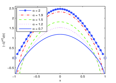
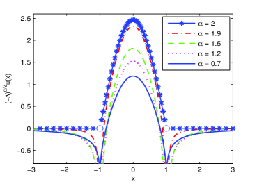
Figure 1: The function $(-\Delta)^{\alpha/2}u(x)$ for various $\alpha$, where ‘o’ represents the points where the function $(-\Delta)^{\alpha/2}u$ does not exist. The displayed domain: (a) $x\in(-1,1)$; (b) $x\in(-3,3)$. It shows that $u(x)$ in (4.3) is an eigenfunction of the standard linear Schrödinger equation in an infinite potential well, but it is not an eigenfunction of the fractional Schrödinger equation.

are computed using the method proposed in Section 3. For simplicity, in Figure 1 we use $\alpha=2$ to represent the result of $-\Delta u$. For $x\in(-1,1)$, Figure 1 (a) shows that the function $-\Delta u(x)$ is always positive, and moreover it has the same shape as $u(x)$. However, if $\alpha<2$, the function $(-\Delta)^{\alpha/2}u(x)$ becomes negative near the boundaries $x=\pm 1$, and $(-\Delta)^{\alpha/2}u(x)\neq cu(x)$ for any constant $c$. Furthermore, Figure 1 (b) shows that when $\alpha<2$, the function $(-\Delta)^{\alpha/2}u(x)$ is not always zero for $x\in{\mathbb{R}}\backslash[-1,1]$, albeit $u(x)\equiv 0$, which is completely different from the case of the standard Laplacian. Since when $\alpha<2$ there is no nonzero constant $c$ satisfying $(-\Delta)^{\alpha/2}u(x)=cu(x)$ for $x\in(-1,1)$ or $x\in{\mathbb{R}}\backslash[-1,1]$, $u(x)$ cannot be an eigenfunction of the fractional linear Schrödinger equation in an infinite potential well [29, 20]. For more discussions, see Sections 4.2.

In Sections 4.2–4.3, the ground and first excited states of the fractional linear Schrödinger equation in an infinite potential well are studied by numerically solving the fractional gradient flow in (3)–(3.3) with $\beta=0$. In our simulations, we choose $L=1$, equivalently, $\Omega=(-1,1)$ and $\Omega_{b}=[-3,-1]\cup[1,3]$. The mesh size is $h=1/4096$, and the time step is $\Delta t=0.005$. The initial condition is chosen as

$$\varphi(x)=\sin\left[\frac{(s+1)\pi}{2}(1+x)\right],\quad\ x\in\Omega,\qquad s=0\ \mbox{or}\ 1,$$ (4.5)

where we choose $s=0$ for computing the ground states, respectively, $s=1$ for the first excited states. We choose the tolerance $\varepsilon=10^{-5}$ in (3.19). In the following, we will use the subscripts “g” and “1” to represent the ground states and the first excited states, respectively, and only the results inside of the infinite potential well (i.e., for $x\in\Omega$) will be displayed, since $\phi(x)\equiv 0$ for $x\notin\Omega$.

4.2 Ground states

Figure 2 depicts the wave function $\phi_{g}(x)$ of the ground states of the fractional linear Schrödinger equation in an infinite potential well for various $\alpha$.

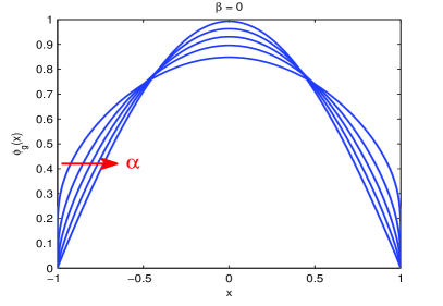
(a) (b)

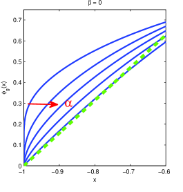
Figure 2: Ground states of the fractional linear ($\beta=0$) Schrödinger equation for $\alpha=0.2,0.7,1.1,1.5$, and $1.9$, where the arrow indicates the change in the wave function for progressively increasing $\alpha$. The plot in (b) shows the change of the wave function near the boundary $x=-1$, the green dotted line $y=\frac{\pi}{2}(1+x)$ is presented for the sake of comparison. The wave function $\phi_{g}(x)$ approaches $\sin[\pi(1+x)/2]$ as $\alpha\to 2$, and its density near the boundaries is large if $\alpha$ is small.

The wave function of the ground state is symmetric with respect to the center of the potential well $x=0$, i.e., $\phi_{g}(x)=\phi_{g}(-x)$ for $x\in(-1,1)$. The wave function monotonically increases for $x\in(-1,0)$ and monotonically decreases for $x\in(0,1)$, and it reaches the maximum value at $x=0$. Furthermore, the ground state of the fractional Schrödinger equation in an infinite potential well depends significantly on the parameter $\alpha$. If $\alpha$ is small, the nonlocal interactions from the fractional Laplacian are strong, resulting in a flatter shape of the wave function. While if $\alpha\to 2$, the wave function of the ground state converges to $\phi_{g}(x)=\sin\big{[}\pi(1+x)/2\big{]}$ – the ground state solution of the standard Schrödinger equation. In addition, Figure 2 (b) shows that the wave function changes quickly around $x=\pm 1$. The smaller the parameter $\alpha$, the larger the density of the wave function near the boundaries.

Our observation suggests that the eigenfunctions of the fractional linear Shcrödinger equation in an infinite potential well differ from those of the standard Schrödingier equation, which confirms the conclusions made in [29, 20]. Furthermore, our numerical results in Figure 2 are consistent with the ground states reported in [41], which were obtained from solving the eigenvectors of a large Toeplitz matrix representing the discrete fractional Laplacian. However, our numerical method converges much faster. Moreover, our method can be used to compute the ground and first excited states of the fractional Schrödinger equation not only in the linear cases but also in the nonlinear cases.

To further understand the properties of the ground states, we define the expected value of position for the $s$-th stationary state as

$$\langle x\rangle_{s}=\int_{\mathbb{R}}x\,|\phi_{s}(x)|^{2}dx=\int_{\Omega}x\,|\phi_{s}(x)|^{2}dx,\qquad s\in{\mathbb{N}}^{0},$$ (4.6)

and the variance in position as

$$\qquad{\rm Var}_{s}(x)=\int_{\mathbb{R}}\big{(}x-\langle x\rangle_{s}\big{)}^{2}\,|\phi_{s}(x)|^{2}dx=\int_{\Omega}\big{(}x-\langle x\rangle_{s}\big{)}^{2}\,|\phi_{s}(x)|^{2}dx,\qquad s\in{\mathbb{N}}^{0}.$$ (4.7)

For the standard linear Schrödinger equation, the expected value of position of the $s$-th stationary state and its variance can be exactly computed from (2.9):

$$\langle x\rangle_{s}=0\quad\ \ \mbox{and}\quad\ \ {\rm Var}_{s}(x)=\frac{L^{2}}{3}\left(1-\frac{6}{\pi^{2}(s+1)^{2}}\right),\qquad s\in{\mathbb{N}}^{0},$$ (4.8)

that is, for any $s\in{\mathbb{N}}^{0}$, the average position is always at $x=0$ – the center of the infinite potential well. The variance in position increases as $s$ increases, and as $s\to\infty$, the variance ${\rm Var}_{s}(x)\to L^{2}/3$. While in the fractional cases,

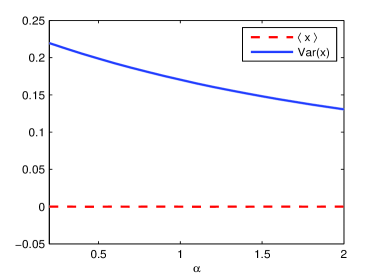
Figure 3: The expected value of position and its variance of the ground state solutions of the fractional linear Schrödinger equation. The expected value of position is zero for any $\alpha\in(0,2)$. The smaller the parameter $\alpha$, the stronger the nonlocal interactions, and thus the larger the scattering of particles, resulting in a larger variance in position.

Figure 3 shows the expected value of position in the ground state and its variance. Due to the symmetry of the wave function $\phi_{g}(x)$ with respect to $x=0$, the expected value of the position $\langle x\rangle_{g}\equiv 0$, independent of the parameter $\alpha$. However, the variance in position highly depends on the parameter $\alpha$. The smaller the parameter $\alpha$, the larger the variance in position. In fact, when $\alpha$ decreases, the nonlocal interactions represented by the fractional Laplacian become stronger, resulting in a larger scattering of particles. Hence, the decrease in the parameter $\alpha$ leads to an increase in the variance in position.

In Table 1, we present our simulated eigenvalues $\mu_{g}^{h}$ of the ground states and compare them with the lower and upper bound estimates in [1] and the asymptotic approximation $\mu_{g}^{a}$ in [23]. Note that in the linear case (i.e., $\beta=0$), the eigenvalue $\mu_{s}$ is equal to the energy $E_{s}$ for any $\alpha\in(0,2]$ and $s\in{\mathbb{N}}^{0}$. From Table 1, we find that the eigenvalue $\mu_{g}$ increases as $\alpha\geq 0.3$ increases, and as $\alpha\to 2$, it converges to $\mu_{g}=\pi^{2}/4$ – the eigenvalue of the ground states of the standard linear Schrödinger equation.

$\alpha$	$\mu_{g}^{\rm lower}$ in [1]	$\mu_{g}^{h}$	$\mu_{g}^{\rm upper}$in [1]	$\mu_{g}^{a}$ in [23]	$|\mu_{g}^{h}-\mu_{g}^{a}|$
0.1	0.9514	0.9726	0.9786	0.9809	0.0083
0.2	0.9182	0.9575	0.9675	0.9712	0.0137
0.3	0.8975	0.9528	0.9655	0.9699	0.0172
0.5	0.8862	0.9702	0.9862	0.9908	0.0206
0.7	0.9086	1.0203	1.0383	1.0418	0.0215
0.9	0.9618	1.1032	1.1227	1.1241	0.0209
1	1	1.1578	$3\pi/8$	$3\pi/8$	0.0203
1.1	1.0465	1.2222	1.2432	1.2415	0.0194
1.3	1.1667	1.3837	1.4064	1.4007	0.0170
1.5	1.3293	1.5976	1.6223	1.6114	0.0138
1.7	1.5447	1.8779	1.9053	1.8873	0.0094
1.9	1.8274	2.2441	2.2747	2.2477	0.0036
1.99	1.9817	2.4437	2.4761	2.4441	0.0004

Table 1: The eigenvalue $\mu_{g}$ of the ground states of the fractional linear ($\beta=0$) Schrödinger equation in an infinite potential well. $\mu^{h}_{g}$ represents our numerical results, $\mu_{g}^{a}=\left(\frac{\pi}{2}-\frac{(2-\alpha)\pi}{8}\right)^{\alpha}$ is the asymptotic approximation obtained in [23], and $\mu_{g}^{\rm lower}$ and $\mu_{g}^{\rm upper}$ are the lower and upper bounds estimated in [1], respectively. It shows that our numerical results $\mu_{g}^{h}$ are consistent with the analytical estimates provided in [1, 23], and as $\alpha\to 2$, the eigenvalue $\mu_{g}\to\pi^{2}/4$ – the eigenvalue of the ground states of the standard linear Schrödinger equation.

Our numerical results are consistent with the lower and upper bounds estimates of the eigenvalues provided in [1, 9, 7], i.e., $\mu_{g}^{h}\in[\mu_{g}^{\rm lower},\mu_{g}^{\rm upper}]$ for any $\alpha\in(0,2)$. Moreover, our results suggest that for the eigenvalues of the ground states, the lower and upper bounds obtained in [1] are much sharper than those in [9, 7]. In addition, we compare our numerical results with the asymptotic approximation $\mu_{g}^{a}=[\pi/2-(2-\alpha)\pi/8]^{\alpha}$ obtained in [23] and find that the asymptotic results are more accurate as $\alpha\to 2$.

4.3 The first excited states

Figure 4 depicts the wave function $\phi_{1}(x)$ of the first excited states of the fractional linear Schrödinger equation in an infinite potential well for various $\alpha$. It shows that the wave function $\phi_{1}(x)$ varies for different values of $\alpha$, and as $\alpha\to 2$, it converges to $\phi_{1}(x)=\sin(\pi(1+x))$ – the first excited state solution of the standard linear

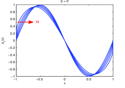
(a) (b)

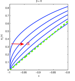
Figure 4: The first excited states of the fractional linear Schrödinger equation for $\alpha=0.2,0.7,1.1,1.5$, and $1.9$, where the arrow indicates the change in the wave function for progressively increasing $\alpha$. The plot in (b) shows the change of the wave function near the boundary $x=-1$, the green dotted line $y=\pi(1+x)$ is presented for the sake of comparison. The wave function $\phi_{1}(x)$ approaches $\sin[\pi(1+x)]$ as $\alpha\to 2$, and its density near the boundaries is large if $\alpha$ is small.

Schrödinger equation in an infinite potential well. In addition, the wave function $\phi_{1}(x)$ of the first excited states is antisymmetric with respect to the center of the infinite potential well $x=0$, i.e., $\phi_{1}(x)=-\phi_{1}(-x)$ for $x\in(-1,1)$ and $\phi(0)=0$. For the standard linear Schrödinger equation, $\phi_{1}(x)$ is also symmetric on each subinterval $(-1,0)$ and $(0,1)$, but in the fractional cases the wave function loses the symmetry in subintervals.

Denote $\rho_{1}(x)=|\phi_{1}(x)|^{2}$ as the position density of the first excited states. The fact that $\phi_{1}(x)$ is antisymmetric about the center of the potential well implies that the position density $\rho_{1}(x)$ is symmetric with respect to $x=0$. Furthermore, there exist two points ${x}_{c}\in(0,1)$ and $-x_{c}\in(-1,0)$ at which the density function $\rho_{1}(x)$ reaches its maximum values,

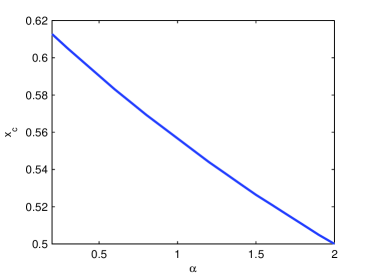
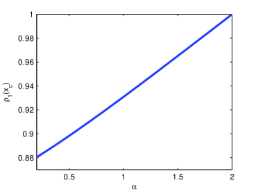
Figure 5: (a) The point $x_{c}$ versus the parameter $\alpha$. (b) The maximum value $\rho_{1}(x_{c})$ versus the parameter $\alpha$.

i.e., $\rho_{1}(x_{c})=\rho_{1}(-x_{c})=\max_{x\in[-1,1]}\{\rho_{1}(x)\}$. The point $x_{c}$ varies for different parameter $\alpha$. Figure 5 shows the values of $x_{c}$ and $\rho_{1}(x_{c})$ for various $\alpha$. We see that the larger the parameter $\alpha$, the smaller the value of $x_{c}$, but the larger the density function $\rho_{1}(x_{c})$, and the maximum value $\rho_{1}(x_{c})$ increases almost linearly as the parameter $\alpha$. In particular, in the first excited states of the standard linear Schrödinger equation, the point $x_{c}=\frac{1}{2}$ and the maximum density function $\rho_{1}(\pm\frac{1}{2})=1$.

In addition, Figure 6 shows the expected value of position and its variance in the first excited states. For any $\alpha\in(0,2)$, the expected value $\langle x\rangle_{1}\equiv 0$, due to the antisymmetry of the wave function $\phi_{1}(x)$, while the variance in position changes for different $\alpha$.

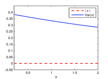
Figure 6: The expected value of position and its variance of the first excited states of the fractional linear Schrödinger equation. The expected value of position is zero for any $\alpha\in(0,2)$. The smaller the parameter $\alpha$, the stronger the nonlocal interactions, and thus the larger the scattering of particles, resulting in a larger variance in position.

The smaller the parameter $\alpha$, the stronger the scattering of particles, and thus the larger the variance in position, which is similar to our observation in Figure 3 for the ground states. However, we find that for a fixed $\alpha$, the variance ${\rm Var}_{1}(x)>{\rm Var}_{g}(x)$. In fact, the energy of the first excited states is higher than that of the ground states, and consequently the scattering of particles in the first excited states is stronger, which leads to a larger variance of the first excited states.

Table 2 shows the eigenvalues of the first excited states, where $\mu_{1}^{h}$ represents our numerical results, $\mu_{1}^{a}=\left[\pi-{(2-\alpha)\pi}/{8}\right]^{\alpha}$ is the asymptotic approximation reported in [23], and $\mu_{1}^{\rm lower}$ and $\mu_{1}^{\rm upper}$ are the lower and upper bound estimates provided in [7, 9], respectively. We find that the eigenvalue of the first excited states increases as $\alpha$ increases, and as $\alpha\to 2$, it converges to $\mu_{1}=\pi^{2}$ – the eigenvalue of the first excited states of the standard linear Schrödinger equation in an infinite potential well. Our numerical results $\mu_{1}^{h}$ are consistent with the estimates obtained in [9, 7] as well as the asymptotical approximations $\mu_{1}^{a}$ reported in [23]. Furthermore, our results suggest that the asymptotic results in [23] are more accurate for the first excited states than for the ground states, as the asymptotic approximation $\mu_{1}^{a}$ has the error $O\left((2-\alpha)/(s+1)\sqrt{\alpha}\right)$ for $s\in{\mathbb{N}}^{0}$.

$\alpha$	$\mu_{1}^{\rm lower}$ in [7, 9]	$\mu_{1}^{h}$	$\mu_{1}^{\rm upper}$ in [7, 9]	$\mu_{1}^{a}$ in [23]	$|\mu_{1}^{h}-\mu_{1}^{a}|$
0.1	0.5606	1.0922	1.1213	1.0913	0.0009
0.2	0.6286	1.1966	1.2573	1.1948	0.0018
0.3	0.7049	1.3148	1.4098	1.3132	0.0026
0.5	0.8862	1.6016	1.7725	1.5977	0.0039
0.7	1.1142	1.9733	2.2285	1.9683	0.0050
0.9	1.4009	2.4583	2.8018	2.4526	0.0057
1	$\pi/2$	2.7549	$\pi$	$7\pi/8$	0.0060
1.1	1.7613	3.0954	3.5226	3.0892	0.0062
1.3	2.2144	3.9380	4.4289	3.9319	0.0061
1.5	2.7842	5.0600	5.5683	5.0545	0.0055
1.7	3.5005	6.5646	7.0009	6.5605	0.0041
1.9	4.4010	8.5959	8.8021	8.5942	0.0017
1.99	4.8786	9.7332	9.7573	9.7330	0.0002

Table 2: The eigenvalue $\mu_{1}$ of the first excited states of the fractional linear Schrödinger equation in an infinite potential well. $\mu^{h}_{1}$ represents our numerical results, $\mu_{1}^{a}=\left(\pi-\frac{(2-\alpha)\pi}{8}\right)^{\alpha}$ is the asymptotic approximation obtained in [23], and $\mu_{1}^{\rm lower}=\pi^{\alpha}/2$ and $\mu_{1}^{\rm upper}=\pi^{\alpha}$ are the lower and upper bounds estimated in [7, 9], respectively. It shows that our numerical results $\mu_{1}^{h}$ are consistent with the analytical estimates obtained in [7, 9, 23], and as $\alpha\to 2$, the eigenvalue $\mu_{1}\to\pi^{2}$ – the eigenvalue of the first excited states of the standard linear Schrödinger equation.

5 Fractional nonlinear Schrödinger equation

There have been many discussions on the stationary states (or eigenfunctions) of the fractional linear Schrödinger equation in an infinite potential well based on different representations of the fractional Laplacian $-(-\Delta)^{\alpha/2}$. However, to the best of our knowledge, no study has been reported in the nonlinear ($\beta\neq 0$) cases yet. In this section, we numerically study the ground and first excited states of the fractional Schrödinger equation with repulsive nonlinear interactions (i.e., $\beta>0$) and attempt to understand the effects of the local (or short-range) interactions and the competition of the local and nonlocal interactions. In our simulations, we choose $L=1$, the mesh size $h=1/4096$, the time step $\Delta t=0.005$, and the convergence tolerance $\varepsilon=10^{-5}$ in (3.19). The initial condition is chosen as defined in (4.5).

5.1 Ground states

Figure 7 shows the wave function $\phi_{g}(x)$ of the ground states of the fractional nonlinear Schrödinger equation in an infinite potential well for various $\alpha$ and $\beta$.

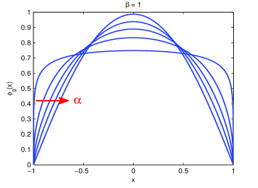
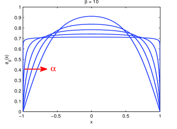
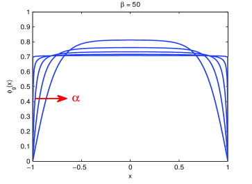
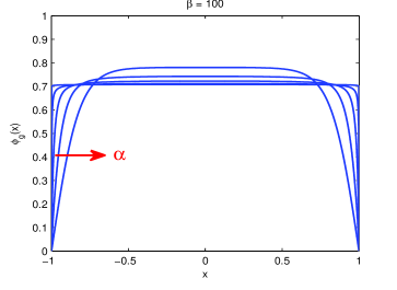
Figure 7: Ground states of the fractional nonlinear Schrödinger equation for $\alpha=0.2,0.7,1.1,1.5$, and $1.99$, where the arrow indicates the change in the wave function for progressively increasing $\alpha$. Boundary layers exist if $\alpha$ is small or $\beta$ is large.

The wave function of the ground states $\phi_{g}(x)$ is always symmetric with respect to the center of the infinite potential well $x=0$. As $\alpha\to 2$, the wave function converges to the ground state solution of the standard Schrödinger equation with the same nonlinear parameter $\beta$. In contrast to the linear cases, the local repulsive interactions may lead to boundary layers in the ground states. Here, we divide our discussions into two interaction regimes: the weak interactions when $\beta\sim o(1)$ and the strong interactions when $\beta\gg 1$. For $\beta\sim o(1)$, the effects of local repulsive interactions are significant only when $\alpha$ is small, resulting in two boundary layers at $x=\pm 1$ (cf. the case of $\alpha=0.2$ and $\beta=1$ in Figure 7). While in the strongly interacting cases (e.g. $\beta=50$ or $100$), the local interactions become significant for any $\alpha\in(0,2)$. Due to the normalization condition, the wave function $\phi_{g}(x)$ inside the potential well tends to approach the value $\sqrt{2}/2$. However, since the wave function $\phi_{g}(x)\equiv 0$ at $x=\pm 1$, two layers emerge at the boundaries of the potential well.

In addition, Figure 7 shows that the width of the boundary layers depends on both $\alpha$ and $\beta$, and either increasing $\beta$ or decreasing $\alpha$ can lead to the thinner boundary layers. That is, with the presence of the local interactions, the strong local or nonlocal interactions can cause a sharp change in wave functions near the boundaries. To further understand this phenomenon, we define $w$ as the width of the boundary layers in the ground states.

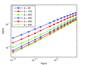
(a) (b)

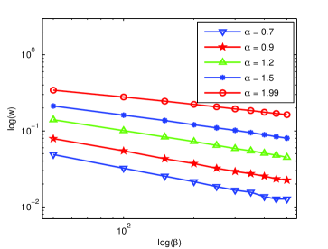
Figure 8: Log-log plots of: (a) the width of boundary layers versus $\alpha$, and (b) the width of boundary layers versus $\beta$, in the ground states of the fractional nonlinear Schrödinger equation in an infinite potential well. It suggests that the width of boundary layers $w$ increases (resp. decreases) as a power function of $\alpha$ (resp. $\beta$).

In our simulations, it is computed by $w=1-|\bar{x}|$, where $\bar{x}$ satisfies

$$\left|\frac{\partial\phi_{g}(x)}{\partial x}\Big{|}_{x=\bar{x}}\right|=\eta,\qquad\mbox{with $\eta\sim O(1)$ a constant}.$$

Here, we choose $\eta={\sqrt{2}}/{2}$. In Figure 8, we present the log-log plots of the width of the boundary layers $w$ versus the parameter $\alpha$ and $\beta$. On the one hand, Figure 8 (a) shows that when $\beta$ is fixed, $\log(w)$ linearly increases as $\log(\alpha)$ increases, and thus we have

$$w=c\alpha^{p},\qquad\mbox{where $c$ and $p>0$ are constants.}$$ (5.9)

The constant $p$ in (5.9) may vary for different parameter $\beta$. On the other hand, Figure 8 (b) shows that when $\alpha$ is fixed, $\log(w)$ linearly decreases as $\log(\beta)$ increases, and

$$w=\frac{d}{\beta^{q}},\qquad\mbox{where $d$ and $q>0$ are constants.}$$ (5.10)

The constant $q$ in (5.9) may be slightly different for various parameter $\alpha$. In particular, the width of the boundary layers $w\sim O\left(1/\sqrt{\beta}\right)$, equivalently, $q=1/2$ in (5.10) for the standard Schrödinger equation [3].

Since the wave function $\phi_{g}(x)$ is symmetric with respect to $x=0$, the expected value of position $\langle x\rangle_{g}\equiv 0$, independent of the parameters $\alpha$ and $\beta$. Here, we omit showing it for brevity. Figure 9 depicts the variance in position of the ground states of the fractional nonlinear Schrödinge equation for various parameters $\alpha$ and $\beta$. It shows that the variance in position monotonically increases as $\alpha$ decreases or $\beta$ increases, implying that the strong local or nonlocal interactions yield a large scattering of particles in the potential well.

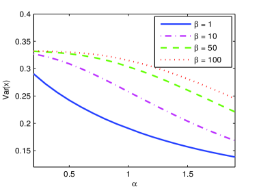
Figure 9: The variance in position of the ground states of the fractional nonlinear Schrödinger equation in an infinite potential well. It increases as the local interaction parameter $\beta$ increases, but decreases as the nonlocal interaction parameter $\alpha$ increases. The variance converges to $1/3$ as $\alpha\to 0$ and $\beta\to\infty$.

Comparing Figure 9 to Figure 3, we find that a small local interaction (e.g., $\beta=1$) can significantly change the variance in position when $\alpha$ is small. In addition, Figure 9 suggests that when $\beta$ is small (e.g., $\beta=1$), the nonlocal interactions from the fractional Laplacian are dominant, and the variance decreases concave up as $\alpha$ increases, similar to the cases of $\beta=0$. When $\beta$ is large, the local repulsive interactions become dominant, and the decrease of the variance becomes concave down as $\alpha$ increases. In addition, due to the constraint $\|\phi_{g}\|^{2}=1$, the variance of position converges to $1/3$ as $\alpha\to 0$ or $\beta\to\infty$.

In Table 3, we present the simulated eigenvalue $\mu_{g}^{h}$ and the kinetic energy $\mu_{g,\rm kin}^{h}$ of the ground states of the fractional nonlinear Schrödinger equation in an infinite potential well, where the kinetic energy $\mu_{g,\rm kin}$ and the interaction energy $\mu_{g,\rm int}$ of the $s$-th stationary state are defined by

$$\mu_{s,\rm kin}=\int_{\mathbb{R}}\phi_{s}^{*}(-\Delta)^{\alpha/2}\phi_{s}\,dx,\qquad\mu_{s,\rm int}=\beta\int_{\mathbb{R}}|\phi_{s}(x)|^{2}dx,\qquad s\in{\mathbb{N}}^{0},$$

respectively. It is easy to see that the eigenvalue $\mu_{s}=\mu_{s,\rm kin}+\mu_{s,\rm int}$, and when $\beta=0$, we have $\mu_{s}\equiv\mu_{s,\rm kin}$ for any $\alpha\in(0,2]$.

$\alpha$	$\beta=1$		$\beta=5$		$\beta=10$		$\beta=50$
	$\mu_{g,\rm kin}^{h}$	$\mu_{g}^{h}$	$\mu_{g,\rm kin}^{h}$	$\mu_{g}^{h}$	$\mu_{g,\rm kin}^{h}$	$\mu_{g}^{h}$	$\mu_{g,\rm kin}^{h}$	$\mu_{g}^{h}$
0.3	0.9625	1.4860	0.9834	3.5006	0.9912	6.0028	1.0002	26.006
0.5	0.9806	1.5291	1.0211	3.5861	1.0463	6.1037	1.0949	26.125
0.7	1.0302	1.6052	1.0860	3.7289	1.1325	6.2862	1.2619	26.393
0.9	1.1122	1.7138	1.1783	3.9224	1.2454	6.5442	1.4862	26.846
1	1.1662	1.7813	1.2359	4.0373	1.3124	6.7001	1.6158	27.150
1.1	1.2299	1.8582	1.3020	4.1647	1.3873	6.8736	1.7562	27.506
1.3	1.3902	2.0445	1.4638	4.4586	1.5641	7.2743	2.0690	28.375
1.5	1.6029	2.2824	1.6741	4.8106	1.7850	7.7506	2.4280	29.455
1.7	1.8822	2.5858	1.9477	5.2312	2.0637	8.3110	2.8422	30.754
1.9	2.2474	2.9743	2.3050	5.7366	2.4199	8.9684	3.3249	32.284

Table 3: The simulated eigenvalue $\mu_{g}^{h}$ and the kinetic energy $\mu_{g,\rm kin}^{h}$ of the ground states of the fractional nonlinear Schrödinger equation in an infinite potential well. Both the eigenvalue $\mu_{g}$ and the kinetic energy $\mu_{g}$ increases as $\alpha$ or $\beta$ increases. If $\beta\gg 1$, the eigenvalue $\mu_{g}\sim O(\beta/2)$.

Table 3 shows that both the eigenvalue $\mu_{g}$ and the kinetic energy $\mu_{g,\rm kin}$ increase as the parameter $\alpha$ or $\beta$ increases. Comparing Tables 1 and 3, we find that for a fixed $\alpha$, the kinetic energy $\mu_{g,\rm kin}$ increases as the local interaction parameter $\beta$ increases. When $\beta$ is small (e.g., $\beta=1$), the kinetic energy is significant in the eigenvalue, while $\beta$ is large (e.g., $\beta=50$), the local interactions become strong, and as a result the energy from the local interactions becomes significant. Furthermore if $\beta\gg 1$, the eigenvalue $\mu_{g}\sim O(\beta/2)$.

5.2 The first excited states

Figure 10 shows the wave function $\phi_{1}(x)$ of the first excited states of

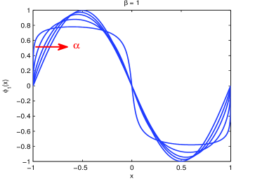
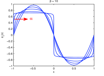
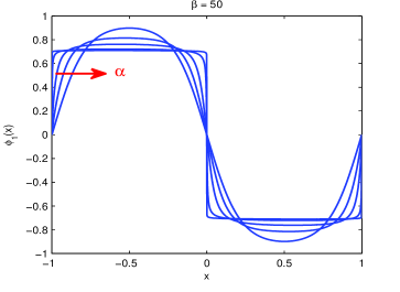
Figure 10: The first excited states of the fractional nonlinear Schrödinger equation for $\alpha=0.2,0.7,1.1,1.5$, and $1.99$, where the arrow indicates then change in the wave function for progressively increasing $\alpha$. When $\alpha$ is small or $\beta$ is large, boundary layers exist at $x=\pm 1$ and one inner layer emerges at $x=0$.

the fractional nonlinear Schrödinger equation in an infinite potential well. The wave function $\phi_{1}(x)$ is antisymmetric with respect to the center of the potential well $x=0$, independent of the parameters $\alpha$ and $\beta$. As $\alpha\to 2$, the wave function converges to the first excited state solution of the standard Schrödinger equation with the same nonlinear parameter $\beta$. The effect of local interactions becomes more significant when $\alpha$ is small, resulting in sharp boundary layers at $x=\pm 1$ as well as one inner layer at $x=0$. The width of the boundary and inner layers decreases as $\alpha$ decreases or $\beta$ increases. Numerical simulations show that our method converges fast in computing both the ground and first excited states.

In addition, Figure 11 shows the variance in position of the first excited states of the fractional nonlinear Schrödinger equation for different parameters $\alpha$ and $\beta$.

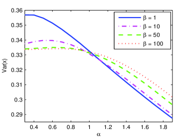
Figure 11: The variance in position of the first excited states of the fractional nonlinear Schrödinger equation in an infinite potential well. It increases as the parameter $\alpha$ decreases. The variance converges to $1/3$ as $\alpha\to 0$ and $\beta\to\infty$.

Note that the expected value of position $\langle x\rangle_{1}\equiv 0$, independent of the parameters $\alpha$ and $\beta$. The properties of the variance in position can be divided into two cases: when $\alpha<1$, the larger the parameter $\beta$, the smaller the variance. As $\beta\to\infty$, the variance converges to $1/3$. When $\alpha>1$, the larger the parameter $\beta$, the bigger the variance, implying that in this case the scattering of particles is mainly contributed by the local repulsive interactions.

In Table 4, we present the numerical results of the eigenvalue $\mu_{1}^{h}$ and the kinetic energy $\mu_{1,\rm kin}$ of the first excited states for various $\alpha$ and $\beta$.

$\alpha$	$\beta=1$		$\beta=5$		$\beta=10$		$\beta=50$
	$\mu_{1,\rm kin}^{h}$	$\mu_{1}^{h}$	$\mu_{1,\rm kin}^{h}$	$\mu_{1}^{h}$	$\mu_{1,\rm kin}^{h}$	$\mu_{1}^{h}$	$\mu_{1,\rm kin}^{h}$	$\mu_{1}^{h}$
0.3	1.3347	1.8994	1.3919	3.9536	1.4193	6.4629	1.4544	26.471
0.5	1.6176	2.2248	1.7011	4.3873	1.7670	6.9514	1.9258	27.036
0.7	1.9850	2.6253	2.0763	4.9161	2.1727	7.5807	2.5141	27.932
0.9	2.4665	3.1325	2.5532	5.5554	2.6681	8.3519	3.2042	29.195
1	2.7616	3.4385	2.8430	5.9257	2.9622	8.7962	3.5912	29.968
1.1	3.1009	3.7874	3.1754	6.3365	3.2960	9.2847	4.0113	30.835
1.3	3.9416	4.6449	4.0007	7.3079	4.1145	10.417	4.9744	32.866
1.5	5.0624	5.7798	5.1062	8.5416	5.2040	11.809	6.1553	35.321
1.7	6.5661	7.2961	6.5970	10.141	6.6742	13.554	7.6466	38.255
1.9	8.5968	9.3383	8.6180	12.254	8.6749	15.793	9.5898	41.752

Table 4: The simulated eigenvalue $\mu_{1}^{h}$ and the kinetic energy $\mu_{1,\rm kin}^{h}$ of the first excited states of the fractional nonlinear Schrödinger equation in an infinite potential well. Both the eigenvalue and the kinetic energy increases as $\alpha$ or $\beta$ increases.

It shows that both the eigenvalue and kinetic energy increase as the parameter $\alpha$ or $\beta$ increases. Comparing Tables 4 and 3, we find that for fixed parameters $\alpha$ and $\beta$, the kinetic energy $\mu_{1,\rm kin}$ of the first excited states is much larger than $\mu_{g,\rm kin}$ of the ground states, which mainly caused by the emergence of the inner layer in the first excited states. Similar to the cases of the ground states, the kinetic energy is significant in the eigenvalue only when the local interaction is weak (i.e., $\beta$ is small).

6 Conclusion and discussion

Due to the non-locality of the fractional Laplacian, it is very challenging to solve the eigenvalues and eigenfunctions of the fractional Schrödinger equation in an infinite potential well. We proposed an efficient and accurate numerical method to compute the ground and first excited states of the one-dimensional (1D) fractional Schrödinger equation in an infinite potential well, based on the integral representation of the fractional Laplacian $-(-\Delta)^{\alpha/2}$. Taking the nonlocal character of the fractional Laplacian into account, we introduced the nonzero volume constraint to the fractional Schrödinger equation in a bounded domain. To compute its ground and first excited states, we proposed a fractional gradient flow with discrete normalization and discretized it by the trapezoidal type quadrature rule method in space and the semi-implicit Euler method in time. Our method can be used to compute the ground and first excited states for both linear and nonlinear fractional Schrödinger equation. It can be also applied to study the fractional partial differential equations (PDEs) with Riesz fractional derivatives in space.

To demonstrate the effectiveness of our numerical method, on the one hand, we studied the ground and first excited states in the linear ($\beta=0$) cases. Our numerical results suggested that the eigenfunctions of the fractional Schrödinger equation are significantly different from those of the standard Schrödinger equations. The nonlocal interactions are strong when $\alpha$ is small, leading to large scattering of particles in the infinite potential well. Compared to the ground states, the scattering of particles in the first excited states is stronger because of its larger energy. In addition, we compared our simulated eigenvalues with the estimates obtained in [7, 9, 1, 23] and found that the asymptotic approximations obtained in [23] are more accurate when $\alpha\to 2$. The estimates of lower and upper bounds of the eigenvalues in [7, 9] are valid for both ground and first excited states, however, the estimates obtained in [1] for the ground states are much sharper.

On the other hand, we studied the ground and first excited states in the nonlinear cases with $\beta>0$. It showed that the eigenvalues of both ground and first excited states monotonically increase as the parameter $\alpha$ or $\beta$ increases. However, the presence of the local interactions in the fractional Schrödinger equation significantly changes the wave functions, especially when $\alpha$ is small. Boundary layers emerge in the ground states, and additionally one inner layer exists in the first excited states. The width of the boundary layers depends on both the local interaction parameter $\beta$ and the nonlocal interaction parameter $\alpha$. More precisely, if $\beta$ is fixed, the width of the boundary layers increases as a power function of $\alpha$; while if $\alpha$ is fixed, the width decreases as a power function of $\beta$. For the standard nonlinear Schrödinger equation, the width of the boundary layers is $O(1/\sqrt{\beta})$ [3]. In addition, the expected value of position is always zero, independent of the parameters $\alpha$ and $\beta$. However, the variance in position increases as $\alpha$ decreases or $\beta$ increases, implying that strong local or nonlocal interactions result in the large scattering of particles. As $\alpha\to 0$ or $\beta\to\infty$, the variance in position convergences to $1/3$.

Acknowledgements The authors would like to thank Dr. John Burkardt and Dr. Qiang Du for their valuable comments to improve the paper.

References

- [1] R. Bauelos and T. Kulczycki, The Cauchy process and the Steklov problem, J. Funct. Anal., 211 (2004), pp. 355–423.
- [2] W. Bao and Q. Du, Computing the ground state solution of Bose–Einstein condensates by a normalized gradient flow, SIAM J. Sci. Comput., 25 (2004), pp. 1674–1697.
- [3] W. Bao, F. Y. Lim and Y. Zhang, Energy and chemical potential asymptotics for the ground state of Bose–Einstein condensates in the semiclassical regime, Bulletin of the Institute of Mathematics, 2 (2007), pp. 495–532.
- [4] S. S. Bayin, On the consistency of the solutions of the space fractional Schrödinger equation, J. Math. Phys., 53 (2012), 042105.
- [5] S. S. Bayin, Comment on “On the consistency of the solutions of the space fractional Schrödinger equation”, J. Math. Phys., 54 (2013), 074101.
- [6] X. Chang, Ground state solutions of asymptotically linear fractional Schrödinger equations, J. Math. Phys., 54 (2013), 061504.
- [7] Z. -Q. Chen and R. Song, Two-sided eigenvalue estimates for subordinate processes in domains, J. Funct. Anal., 226 (2005), pp. 90–113.
- [8] M. L. Chiofalo, S. Succi and M. P. Tosi, Ground state of trapped interacting Bose-Einstein condensates by an explicit imaginary-time algorithm, Phys. Rev. E, 62 (2000), pp. 7438–7444.
- [9] R. D. Deblassie, Higher order PDEs and symmetric stable processes, Probab. Theory Rel., 129 (2004), pp. 495–536.
- [10] M. D’Elia and M. Gunzburger, The fractional Laplacian operator on bounded domains as a special case of the nonlocal diffusion operator, Comput. Math. Appl., 66 (2013), pp. 1245–1260.
- [11] J. Dong, Lévy path integral approach to the solution of the fractional Schrödinger equation with infinite square well, (2013), arXiv: 1301.3009v1.
- [12] J. Dong and M. Xu, Some solutions to the space fractional Schrödinger equation using momentum representation method, J. Math. Phys., 48 (2007), 072105.
- [13] Q. Du, M. Gunzburger, R. B. Lehoucq and K. Zhou, Analysis and approximation of nonlocal diffusion problems with volume constraints, SIAM Rev., 54 (2012), pp. 667–696.
- [14] S. Duo and Y. Zhang, Numerical methods for fractional partial differential equations in bounded domain, in preparation.
- [15] B. Feng, Ground states for the fractional Schrödinger equation, Electron J. Differ. Eq., 2013 (2013), pp. 1–11.
- [16] W. Greiner, Quantum Mechanics: An Introduction, Springer Verlag Gmbh, 2001.
- [17] Q. Guan and Z. Ma, Boundary problems for fractional Laplacians, preprint.
- [18] X. Guo and M. Xu, Some physical applications of fractional Schrödinger equation, J. Math. Phys., 47 (2006), 082104.
- [19] E. Hawkins and J. M. Schwarz, Comment on “On the consistency of solutions of the space fractional Schrödinger equation”, (2012), arXiv: 1210.1447v1.
- [20] R. Herrmann, The fractional Schrödinger equation and the infinite potential well – Numerical results using the Riesz derivative, Gam. Ori. Chron. Phys., 1 (2013), pp. 1–12.
- [21] M. Jeng, S. L.Y. Xu, E. Hawkins and J. M. Schwarz, On the nonlocality of the fractional Schrödinger equation, J. Math. Phys., 51 (2010), 062102.
- [22] K. Kirkpatrick and Y. Zhang, Dynamics of fractional Schrödinger equation and decoherence, (2013), preprint.
- [23] M. Kwaśnicki, Eigenvalues of the fractional Laplace operator in the interval, J. Funct. Anal., 262 (2012), pp. 2379–2402.
- [24] N. S. Landkof, Foundations of Modern Potential Theory, Die Grundlehren der mathematischen Wissenschaften, Band 180. Translated from the Russian by A. P. Doohovskoy. Springer, New York, 1972.
- [25] N. Laskin, Fractional quantum Mechanics and Lévy path integrals, Phys. Lett. A, 268 (2000), pp. 298–305.
- [26] N. Laskin, Fractional quantum mechanics, Phys. Rev. E, 62 (2000), pp. 3135–3145.
- [27] N. Laskin, Fractals and quantum mechanics, Chaos, 10 (2000), pp. 780–790.
- [28] N. Laskin, Fractional Schrödinger equation, Physical Review E, 66 (2002), 056108.
- [29] Y. Luchko, Fractional Schrödinger equation for a particle moving in a potential well, J. Math. Phys., 54 (2013), 012111.
- [30] S. G. Samko, A. A. Kilbas, O. I. Marichev, Fractional Integrals and Derivatives: Theory and applications, Gordon and Breach Science, Amsterdam, 1993.
- [31] S. Secchi, Ground state solutions for nonlinear fractional Schrödinger equations in , J. Math. Phys., 54 (2013).
- [32] E. M. Stein, Singular integrals and differentiability properties of functions, Princeton University Press, Princeton, 30 (1970).
- [33] X. Tian and Q. Du, Analysis and comparison of different approximations to nonlocal diffusion and linear peridynamic equation, SIAM J. Numer. Anal., 51 (2013), pp. 3458–3482.
- [34] V. V. Uchailkin, R. T. Sibatov and V. V. Saenko, Leaky-box approximation to the fractional diffusion model, J. Phys: Conference Series, 409 (2013), 012057.
- [35] E. Valdinoci, From the long jump random walk to the fractional Laplacian, (2009), arXiv: 0901. 3261v1.
- [36] J. L. Vázquez, Nonlinear diffusion with fractional Laplacian operators, in Nonlinear Partial Differential Equations, H. Holden and K. H. Karlsen, ed., The Abel Symposium, 2010, pp. 271–298.
- [37] J. L. Vázquez, Recent progress in the theory of nonlinear diffusion with fractional Laplacian operators, arXiv: 1401.3640v1.
- [38] S. Wang and M. Xu, Generalized fractional Schrödinger equation with space-time fractional derivatives, J. Math. Phys., 48 (2007), 043502.
- [39] Q. Yang, F. Liu, I. Turner, Numerical methods for fractional partial differential equations with Riesz space fractional derivatives, Appl. Math. Model., 34 (2010), pp. 200-218.
- [40] Y. Zhang, Mathematical Analysis and Numerical Simulation for Bose–Einstein condensation, Ph. D Dissertation, National University of Singapore, 2006.
- [41] A. Zoia and A. Rosso, M. Kardar, Fractional Laplacian in bounded domains, Phys. Rev. E, 76 (2007), 021116.