Stochastic dynamics and the noisy Brusselator behaviour

Abstract

In non-linear dynamics there are several model systems to study oscillations. One iconic example is the “Brusselator”, which describes the dynamics of the concentration of two chemical species in the non-equilibrium phase. In this work we study the Brusselator dynamics as a stochastic chemical reaction without diffusion analysing the corresponding stochastic differential equations with thermal or multiplicative noise. In both stochastic scenarios we investigate numerically how the Hopf bifurcation of the non-stochastic system is modified. Furthermore, we derive analytical expressions for the noise average orbits and variance of general stochastic dynamics, a general diffusion relationship in the thermal noise framework, and an asymptotic expression for the noise average quadratic deviations. Hence, besides the impact of these results on the noisy Brusselator’s dynamics, our findings are also relevant for general stochastic systems.

I Introduction

There are many instances in which physical systems spontaneously become emergent or orderly Strogatz ; Murray ; Prigogine . Even more spectacular is the order created by chemical systems; the most dramatic being the order associated with life. However, not all chemical reactions generate order. The class of reactions most closely associated with order creation are the auto-catalytic reactions. These are chemical reactions in which at least one of the reactants is also a product, hence, the equations are fundamentally non-linear due to this feedback effect.

Simple auto-catalytic reactions are known to exhibit sustained oscillations Prigogine ; Broomhead ; Osipov , thus, creating temporal order. Other reactions can generate separation of chemical species generating spatial order, i.a., the Belousov-Zhabotinsky reaction Agladze . More complex reactions are involved in metabolic pathways and networks in biological systems Petsko ; Etay ; Hilborn ; Ciandrini . The transition to order as the distance from equilibrium increases is not usually continuous. Order typically appears abruptly. The threshold between the disorder of chemical equilibrium and order happens as a phase transition. The conditions for a phase transition to occur are determined with the mathematical machinery of non-equilibrium statistical mechanics Reichl .

A paradigmatic example of an auto-catalytic reaction, which exhibits out of equilibrium oscillations, is the “Brusselator”. It describes the dynamics of the concentration of two chemical species, where the evolution of each component is obtained from the following dimensionless differential equations Prigogine ; Murray ; Broomhead ; Osipov

$$\left\{\begin{array}[]{lcl}d\,u/d\,\tau&=&1-\left(b+1\right)\,u+a\,u^{2}\,v=f\left(u,\,v\right)\,,\\ d\,v/d\,\tau&=&b\,u-a\,u^{2}\,v=g\left(u,\,v\right)\,,\end{array}\right.$$ (1)

where $a,\,b>0$ are constants, $u$ and $v$ correspond to the concentrations of the two species, and $\tau$ is the dimensionless time. These differential equations show, for most initial conditions, self-sustained oscillations when $b>1+a$. The transition from the chemical equilibrium state to this oscillatory behaviour happens via a Hopf bifurcation Guckenheimer .

Classical and recent work has emphasized the importance of fluctuations to better model the internal evolution of macroscopic systems which are only accounted for by stochastic models Broomhead ; Osipov ; Agladze ; Petsko ; Traulsen ; Jan ; Melbinger ; Beta ; Abbott . In particular, Chemical oscillations might be augmented and/or disturbed by stochastic effects and random drift. For instance, models of diffusion-driven pattern formation that rely on the Turing mechanism are commonly used in science. Nevertheless, many such models suffer from the defect of requiring fine tuning of parameters in order to predict the formation of spatial patterns. The limited range of parameters for which patterns are seen could be attributed to the simplicity of the models chosen to describe the process; however, for systems with an underlying molecular basis another explanation has recently been put forward Biancalani ; Biancalani2 ; Butler . Those authors have observed that Turing-like patterns exist for a much greater range of parameter values if the discrete nature of the molecules comprising the system is taken into account. The systems within this class may be analysed using the theory of stochastic processes. For the Brusselator, the inclusion of noise affects the concentrations of the relevant chemical species and accounts for the molecular character of the reaction compounds.

In this work, we study the Brusselator system without diffusion as a stochastic process due to the inclusion of thermal or multiplicative noise. We discuss the non-stochastic dynamics of the Brusselator analytically (Sec. II.1) and derive a general expression for the noise average linear and quadratic deviations of the thermal noise stochastic system (Sec. III.1) from generic Stochastic Differential Equations (SDEs). Consequently, we obtain a general Einstein diffusion relationship (Sec. III.2) and derive a general expression for the asymptotic behaviour of the quadratic deviations. These expressions are derived in terms of the eigenvalues and eigenvectors of the Jacobian matrix of the non-stochastic equations. Furthermore, we analyse how the Brusselator Hopf bifurcation is perturbed by thermal or multiplicative noise via numerical experiments (Sec. III.3). Our results show that, in both frameworks, the bifurcation transition is kept in average for small noise intensities ($\Gamma\lesssim 0.1$). Our findings are relevant, not only for the analysis of the noisy Brusselator chemical reaction, but also for general stochastic systems.

II Model

II.1 Dynamical features of the Brusselator

The equilibrium phase of the Brusselator chemical reaction is given by the fixed point (FP) of Eq. (1), namely, $\left(u_{0},\,v_{0}\right)=\left(1,\,b/a\right)$. The Jacobian of Eq. (1) evaluated at the FP is given by

$$D\vec{F}_{(u_{0},\,v_{0})}=\left(\begin{array}[]{cc}b-1&a\\ -b&-a\end{array}\right),$$ (2)

where each entry of the matrix corresponds to the partial derivatives given by $\left(\partial\,f_{i}/\partial\,x_{j}\right)_{(u_{0},\,v_{0})}$, $f_{i}$ being $f_{1}=f$ or $f_{2}=g$, with $x_{1}=u$ and $x_{2}=v$. The eigenvalues $\lambda_{\pm}$ of Eq. (2) are the solutions of the characteristic polynomial $\chi\left(\lambda\right)=\det\left(D\vec{F}_{u_{0},\,v_{0}}-\lambda\,\mathbf{I}\right)=0$, i.e.,

$$\lambda_{\pm}=\frac{\mathsf{Tr}}{2}\pm\sqrt{\frac{\mathsf{Tr}^{2}}{4}-\Delta}\,,$$ (3)

and determine the local stability of the FP. As $\Delta=a>0$, $\Delta$ being the determinant of Eq. (2), a saddle node FP is impossible Guckenheimer . Hence, analysing the sign of the trace [$\mathsf{Tr}=b-\left(1+a\right)$] of Eq. (2), we have that the FP is unstable if $\mathsf{Tr}>0$ and that the FP is stable if $\mathsf{Tr}<0$. The critical point is then $b_{c}\equiv 1+a$.

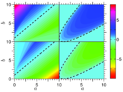
Figure 1: (Color online) Real (left column) and imaginary (right column) parts of the eigenvalue solutions ($\lambda_{\pm}$ in colour code) for the Brusselator Jacobian matrix at the fixed point (FP). The top row panels show $\lambda_{+}$ and the bottom row panels $\lambda_{-}$ [positive and negative solutions of Eq. (3), respectively]. The dashed lines on the left column panels indicate the critical border $b_{c}=1+a$. The FP is stable for values beneath the dashed line, otherwise, is unstable. The dashed lines on the right column panels indicate the border between ordinary (outside the dashed area) and spiral (inside the dashed area) FP.

The square root in Eq. (3) determines if the FP is ordinary ($\lambda_{\pm}\in\mathbb{R}$) or spiral ($\lambda_{\pm}\in\mathbb{C}$). Thus, two two-fold cases appear, as they are shown in Fig. 1 (colour code). From the left column panels in Fig. 1, it is seen that the line $b_{c}=1+a$ (diagonal dashed line) divides the parameter space in an upper positive region ($\mathsf{Re}\{\lambda_{\pm}\}>0$) and a lower negative region ($\mathsf{Re}\{\lambda_{\pm}\}<0$). These two regions account for the unstable and stable FP situations, respectively. On the right column of the figure, the spiral and ordinary characteristics of the FP eigenvalues are discriminated by the critical set $\mathsf{Tr}^{2}=4\Delta$ (curved dashed line). The outer region of this set has the imaginary part null, namely, $\mathsf{Im}\{\lambda_{\pm}\}=0$, thus, the FP is ordinary classified. On the inside region, the FP is spiral (unstable, if it is above the critical level, and stable if it is below).

However, the main feature for self-sustained oscillations to occur is to have an unstable FP ($b>1+a$). In that case, solutions are attracted to a limit-cycle Guckenheimer ; Jan . A limit-cycle on a plane (or a two-dimensional manifold) is a closed trajectory in phase space having the property that at least one other trajectory spirals into it either as time approaches infinity or as time approaches negative infinity Guckenheimer . This behaviour is shown in Fig. 2 for the Brusselator. For $b<b_{c}$ the FP is stable and there is no self-sustained oscillation. Such a steady state solution becomes unstable under a Hopf bifurcation as $b$ is increased. A stable oscillation appears for $b>b_{c}$, which corresponds to the non-equilibrium phase of the system.

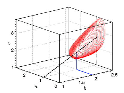
Figure 2: (Color online) Brusselator’s bifurcation diagram as $b$ is increased for $a=1$. Red dots correspond to the system’s asymptotic orbits. The critical point $b_{c}=1+a=2$ is signalled by straight (blue online) lines. The dashed (black online) line corresponds to the steady state solution $\left(1,\,b/a\right)$, which becomes unstable after the critical point as a Hopf bifurcation.

II.2 Stochastic Dynamics

A general coupled set of first order Stochastic Differential Equations (SDEs) is given by

$$\dot{\vec{x}}_{\eta}(t)=\vec{F}\left(\vec{x}_{\eta}(t),\,t\right)+\mathbf{H}\left(\vec{x}_{\eta}(t),\,t\right)\,\vec{\eta}(t)\,,$$ (4)

where we name $\vec{x}_{\eta}=\{x_{i}:\;i=1,\,\ldots,\,N\}$ as the set of state variables, $\vec{F}$ as the deterministic part of the SDE (namely, a field vector $\vec{F}$ with components $f_{i}:\mathbb{R}^{N}\times\mathbb{R}\to\mathbb{R}$ known as the drift coefficients), $\mathbf{H}$ as the $N\times N$ coupling matrix with function entries $h_{ij}:\mathbb{R}^{N}\times\mathbb{R}\to\mathbb{R}$ [i.e., $h_{ij}\left(\vec{x}_{\eta}(t),\,t\right)$], known as the diffusion coefficients, and $\vec{\eta}$ as the vector of random fluctuations. The noise is assumed to be uncorrelated and with zero mean for all coordinates, namely,

$$\left\langle\eta_{i}(t)\,\eta_{j}(s)\right\rangle=\delta_{ij}\,\delta\left(t-s\right)\,,$$

$$\text{and}\;\;\left\langle\eta_{i}(t)\right\rangle=0\,,\;\forall\,i=1,\,\ldots,\,N\,,$$ (5)

where, as in the following, we denote $\left\langle\cdots\right\rangle$ to be the average over various noise realisations (in other words, a mean value over an ensemble of possibly different fluctuations), $\delta_{ij}$ to be the Kronecker delta, and $\delta(t-s)$ to be the Dirac delta function.

The system is said to be subject to additive or thermal noise if the drift coefficients ($h_{ij}$) are constants, otherwise it is said to be subject to multiplicative noise. For the Brusselator, taking into account random fluctuations in the equations of motion modifies the concentrations of the relevant chemical species into stochastic variables. The inclusion of noise is intended to account for the molecular character of the chemical reaction. Hence, the Stochastic Brusselator Equations (SBEs) are

$$\left[\!\begin{array}[]{c}\dot{u}\\ \dot{v}\end{array}\!\right]=\left[\!\begin{array}[]{c}f\left(u,\,v\right)\\ g\left(u,\,v\right)\end{array}\!\right]+\mathbf{H}\left(u,\,v\right)\left[\!\begin{array}[]{c}\eta_{u}\\ \eta_{v}\end{array}\!\right]\,,$$ (6)

with

$$\mathbf{H}\left(u,\,v\right)=\left[\!\begin{array}[]{cc}h_{11}\!\left(u,\,v\right)&h_{12}\!\left(u,\,v\right)\\ h_{21}\!\left(u,\,v\right)&h_{22}\!\left(u,\,v\right)\end{array}\!\right]\,,$$ (7)

where the deterministic drift coefficients come from Eq. (1) and the chemical concentrations $u$ and $v$ are now stochastic variables.

In particular, the analysis of how the stability of the FP (sub-critical parameter values) and the limit-cycle (above criticality) of the deterministic Brusselator changes due to the inclusion of noise is carried by linearising the SBEs around the particular stable solution. We tackle this analysis on the general SDE case [Eq. (4)]. We start by analysing the effect of the noise over the stability of the FP and find that the resulting average solutions are mainly affected by the eigenvalues and eigenvectors of the Jacobian of the field vector $\vec{F}$ and the drift coefficients.

Let $\delta\vec{x}_{\eta}\equiv\vec{x}_{\eta}-\vec{x}_{eq}$ be the deviation vector, where $\vec{x}_{eq}$ is the steady equilibrium solution (FP). Assuming that this deviation is small for all times and any noise realisation, then,

$$\delta\dot{\vec{x}}_{\eta}=\left[D\vec{F}_{\vec{x}_{eq}}+\left(\nabla\left[\mathbf{H}\left(\vec{x}_{\eta}(t),\,t\right)\,\vec{\eta}(t)\right]\right)_{\vec{x}_{eq}}\right]\times$$

$$\times\delta\vec{x}_{\eta}+\mathbf{H}_{\vec{x}_{eq}}\,\vec{\eta}(t)\,,$$ (8)

$D\vec{F}_{\vec{x}_{eq}}$ ($\mathbf{H}_{\vec{x}_{eq}}$) being the Jacobian (coupling) matrix evaluated at the FP and $\nabla$ the gradient operator. Unless the noise is additive, the matrices inside the square brackets have a noise dependence. Thus, we restrict ourselves to the case of thermal noise for the mathematical derivations.

For additive noise, $\mathbf{H}(\vec{x}_{\eta}(t),t)$ is a constant matrix, $\mathbf{H}$, independent of the system’s state vector and time, hence, direct integration of Eq. (8) is possible. Denoting $D\vec{F}_{\vec{x}_{eq}}=\mathbf{J}$, the deviation vector evolves according to

$$\delta\vec{x}_{\eta}(t)=e^{\mathbf{J}\,t}\delta\vec{x}(0)+\int_{0}^{t}ds\;e^{\mathbf{J}\,(t-s)}\,\mathbf{H}\,\vec{\eta}(s)\,.$$ (9)

We note that the exponentials of the Jacobian matrix in the former expressions are understood to be a matrix exponent, thus, they are computed in a power series expansion using its spectral decomposition [$\mathbf{J}=\mathbf{P}\mathbf{\Lambda}\mathbf{P}^{-1}$, where $\left(\mathbf{P}\right)_{ij}=\left(\vec{v}_{j}\right)_{i}$ is the $i$-th coordinate of the $j$-th eigenvector of $\mathbf{J}$ and $\left(\mathbf{\Lambda}\right)_{ij}=\delta_{ij}\lambda_{j}$, with $\lambda_{j}$ being the $j$-th eigenvalue of $\mathbf{J}$]. Specifically,

$$e^{\mathbf{J}\,t}\equiv\sum_{n=0}^{\infty}\frac{1}{n!}\left(\mathbf{J}\,t\right)^{n}=\mathbf{P}\,e^{\mathbf{\Lambda}\,t}\,\mathbf{P}^{-1}\,.$$ (10)

III Results

III.1 Thermal noise ensemble first and second moments

Due to the stochastic character of Eq. (9), we focus on the analytical derivation of the first and second moments of the thermal noise ensemble distribution. In other words, we derive an expression for the noise average value of the deviations with respect to the FP and the noise average value of the quadratic deviations with respect to the FP. The noise average value of the deviations, $\vec{m}(t)\equiv\left\langle\delta\vec{x}_{\eta}(t)\right\rangle$, is

$$\vec{m}(t)=e^{\mathbf{J}\,t}\,\delta\vec{x}(0)+\int_{0}^{t}ds\;e^{\mathbf{J}\,(t-s)}\,\left\langle\mathbf{H}\,\vec{\eta}(s)\right\rangle\,,$$ (11)

and the noise average value of the quadratic deviations, $\rho^{2}(t)\equiv\left\langle\left[\delta\vec{x}_{\eta}(t)\right]^{2}\right\rangle$, is

$$\rho^{2}(t)=e^{\mathbf{J}\,t}\,\delta\vec{x}(0)\cdot e^{\mathbf{J}\,t}\,\delta\vec{x}(0)+$$

$$2e^{\mathbf{J}\,t}\,\delta\vec{x}(0)\cdot\int_{0}^{t}ds\;e^{\mathbf{J}\,(t-s)}\,\left\langle\mathbf{H}\,\vec{\eta}(s)\right\rangle+$$

$$\int_{0}^{t}\!ds\!\int_{0}^{s}\!ds^{\prime}\left\langle e^{\mathbf{J}(t-s)}\,\mathbf{H}\,\vec{\eta}(s)\cdot e^{\mathbf{J}(t-s^{\prime})}\,\mathbf{H}\,\vec{\eta}(s^{\prime})\right\rangle,$$ (12)

where “ $\cdot$ ” is the inner product between vectors. In particular, for the Jacobian eigenvectors we have that $\vec{v}_{n}\cdot\vec{v}_{m}=\sum_{i=1}^{N}\left(\vec{v}_{n}\right)_{i}\left(\vec{v}_{m}\right)_{i}^{\star}=\delta_{nm}$, “ ^⋆ ” being the complex conjugate operation.

As the random fluctuations are additive, then $\mathbf{H}$ is independent of the noise realisation, hence, $\left\langle\mathbf{H}\eta\right\rangle=\mathbf{H}\left\langle\eta\right\rangle=0$. Consequently, the noise average value of the deviations evolves as

$$\vec{m}(t)=\mathbf{P}\,e^{\mathbf{\Lambda}\,t}\,\mathbf{P}^{-1}\,\delta\vec{x}(0)\,,$$ (13)

which is the first main result of this work and constitutes the first moment of the thermal noise ensemble orbits. Equation (13) says that the average of the deviation variables tends to zero for $t\to\infty$ if and only if the eigenvalues correspond to a stable FP, namely, when $\mathsf{Re}\{{\lambda_{i}}\}<0\;\forall\,i$. Hence, the stochastic system returns to the steady state (in average) after being perturbed, as long as the noise intensities are small (i.e., $\left\|\delta\vec{x}_{\eta}(t)\right\|\ll 1$ $\forall\,t$).

In particular, for the Brusselator, the analytical result of Eq. (13) predicts how the noisy chemical concentrations converge to the FP if averaged over various thermal noise realisations, as it is demonstrated in Fig. 3. Both panels show how the analytical prediction (filled squares) of Eq. (13) for $\vec{m}(t)=\left(\left\langle\delta u_{\eta}(t)\right\rangle,\,\left\langle\delta v_{\eta}(t)\right\rangle\right)$ has a remarkable agreement with the numerical experiments, although the initial perturbation is large [the initial condition for every stochastic orbit is $\left(\delta u_{\eta}(0),\,\delta v_{\eta}(0)\right)=\left(0.9,\,-0.9\right)$].

(a)

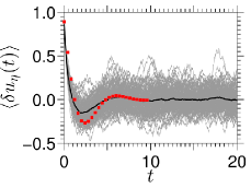
(b)

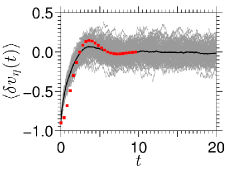
Figure 3: (Color online) Panel (a) [Panel (b)] shows $100$ stochastic orbits of the Brusselator’s chemical concentration deviations from the fixed point $\delta u_{\eta}$ [$\delta v_{\eta}$] in continuous light (grey online) curves. The diffusion coefficients are constant (thermal noise scenario) and given by $h_{ij}=\delta_{ij}\Gamma$, with $\Gamma=10^{-1}$. The noise average orbit deviations in these panels are represented by dark (black online) continuous curves. The analytical predictions [Eq. (13)] for these averages are shown by filled (red online) squares. Both panels corresponds to the sub-critical regime, with $a=b=1$.

On the other hand, the noise average value of the quadratic deviations of the SDE orbits around the steady equilibrium state evolve as

$$\rho^{2}(t)=\delta\vec{x}(0)\cdot\mathbf{P}\,e^{2\mathsf{Re}\{\mathbf{\Lambda}\}\,t}\,\mathbf{P}^{-1}\delta\vec{x}(0)+$$

$$\sum_{i,j,k,n}^{N}h_{ik}\left(\vec{v}_{n}\right)_{i}\left[\frac{e^{2\,\mathsf{Re}\{\lambda_{n}\}\,t}-1}{2\,\mathsf{Re}\{\lambda_{n}\}}\right]\left(\vec{v}_{n}\right)_{j}^{\star}h_{jk}\,,$$ (14)

where $\left(\vec{v}_{n}\right)_{i}$ is the $i$-th coordinate of the eigenvector associated to the $\lambda_{n}$ eigenvalue of the Jacobian matrix in the particular steady state solution and all summations run from $1$ to $N$.

Equation (14) is the second main results in this work and constitutes the second moment of the ensemble of thermal noise realisations. It is derived by applying direct integration of Eq. (12), the noise properties defined in Eq. (5), and the spectral decomposition of the Jacobian matrix [Eq. (10)]. It expresses how the noise and the deterministic part of the SDE produce divergence (or convergence) in the trajectories of neighbouring initial conditions over the ensemble of thermal noise realisations close to the FP solution. The first right hand side term in Eq. (14) diverges (converges) if the FP is unstable (stable). In such case, neighbouring initial conditions are driven away (closer) at a rate given by the real part of the exponents of the system, i.e., by $2\mathsf{Re}\{\lambda_{n}\}$. The second term on the right hand side of Eq. (14) accounts for the divergence (convergence) due to the stochasticity in the system.

In order to find the variance $\sigma^{2}(t)$ of the SDE, it is enough to discard the first term on the right side of Eq. (14). Specifically,

$$\sigma^{2}(t)=\rho^{2}(t)-\vec{m}(t)\cdot\vec{m}(t)=\left\langle\left[\vec{x}_{\eta}(t)\right]^{2}\right\rangle-\left[\left\langle\vec{x}_{\eta}(t)\right\rangle\right]^{2}\,,$$

$$\sigma^{2}(t)=\sum_{i,j,k,n}^{N}{\left(\vec{v}_{n}\right)_{i}h_{ik}\!\left[\frac{e^{2\,\mathsf{Re}\{\lambda_{n}\}\,t}-1}{2\,\mathsf{Re}\{\lambda_{n}\}}\right]\!\left(\vec{v}_{n}\right)_{j}^{\star}h_{jk}}.$$ (15)

III.2 Thermal noise diffusion relationship and the variance asymptotic behaviour

Our general diffusion relationship is derived from Eq. (15) by considering the small time-scales. In such transient window, an expansion in power series up to the first order results in the following Einstein diffusion relationship, $\sigma^{2}(t)\simeq D\,t$,

$$D\equiv\sum_{i,j}^{N}h_{ij}^{2}=\mu\,k_{B}T\,,$$ (16)

where $\mu$ is the mobility coefficient, $k_{B}$ is Boltzmann’s constant, and $T$ is the temperature.

It is worth mentioning that Eq. (16) corresponds to the rate at which the variance of the perturbations grows in time averaged over the various random fluctuation realisations. Hence, it may not be directly relatable to the regular Brownian Motion (BM) solution under an external potential in the over-damped regime, i.e., the known Einstein diffusion relationship Reichl .

On the one hand, the diffusion relationship that BM achieves corresponds to the particle’s position variance, though it depends on the fact that the external force is derived from a potential. However, if the Brusselator field vector ($\vec{F}$) is derived from a bi-dimensional potential, periodic solutions are absent ($\nabla\times\vec{F}=0$), such as the limit-cycle state. On the other hand, the variance relationship for the BM, that holds the Einstein’s diffusion relationship, is a relationship regarding how much the particle diffuses as if it performed random walks as a function of the temperature, i.e., the parameter that regulates the “strength” of the fluctuations. For the Brusselator, the relationship given by Eq. (16), predicts a similar behaviour for the variance of the perturbations in the system out of the equilibrium state when subject to additive noise, but there is no particle movement involved. Instead, the “movement” corresponds to the chemical concentration fluctuations. Consequently, the general diffusion relationship we find is only mentioned as a qualitative Einstein diffusion relationship analogue which exhibits the same mathematical formulation as the one for BM.

For the Brusselator, in the case where the thermal noise only affects each chemical concentration independently, namely, $h_{ij}=\delta_{ij}\Gamma$, then $\sum_{i,j}^{2}h_{ij}^{2}=2\Gamma^{2}$, and Eq. (16) results in

$$D=2\Gamma^{2}=\mu\,k_{B}T\,,$$ (17)

where we can continue the analogy with the BM and say that the $2$ appearing in the relationship corresponds to the $2$ degrees of freedom of the Brusselator.

For a stable FP, the variance [Eq. (15)] saturates at a finite value, meaning that initially neighbouring orbits are found always within a fixed distance from the FP. In other words, for a stable FP, the variance of the thermal noise SDE converges to

$$\lim_{t\to\infty}\sigma^{2}(t)=-\sum_{i,j,k,n}^{N}\left(\vec{v}_{n}\right)_{i}h_{ik}\frac{1}{2\,\mathsf{Re}\{\lambda_{n}\}}\left(\vec{v}_{n}\right)_{j}^{\star}h_{jk}\,,$$ (18)

with $\mathsf{Re}\{\lambda_{n}\}<0\;\forall\,n$. This constitutes the final analytical result of this work.

(a)

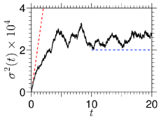
(b)

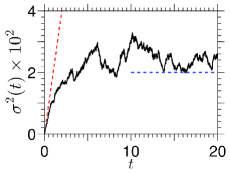
Figure 4: (Color online) The panels show the sub-critical ($a=b=1$) noise average orbits variance, namely, $\sigma^{2}=\left\langle[\vec{x}_{\eta}(t)]^{2}\right\rangle-[\left\langle\vec{x}_{\eta}(t)\right\rangle]^{2}$, by a continuous dark (black online) curve for two noise strength values: $\Gamma=10^{-2}$ [panel (a)] and $\Gamma=10^{-1}$ [panel (b)], with constant diffusion coefficients (thermal noise) given by $h_{ij}=\delta_{ij}\,\Gamma$. The vertical [horizontal] dashed (red online [blue online]) curves represents the transient [asymptotic] analytical prediction of Eq. (16) [Eq. (18)] for the behaviour of $\sigma^{2}$.

For the Brusselator, the asymptotic behaviour of the variance implies that for the sub-critical values of the parameter ($b<b_{c}$), any small deviation from the FP in presence of moderate additive noise keeps, in average, the same asymptotic state. This is also valid for the limit-cycle situation when parameters are above the critical point ($b>b_{c}$) if, in the former equations, we use the Floquet exponents and corresponding time-dependent eigenvectors Guckenheimer .

These results [Eqs. (16) and (18)] are shown in Fig. 4 for the particular case of Eq. (17) with $\Gamma=10^{-2}$ [Fig. 4(a)] and $\Gamma=10^{-1}$ [Fig. 4(b)]. As it is seen from the results, both analytical predictions show good agreement with the numerical experiments. Moreover, the asymptotic diffusion, $\sigma^{2}/\Gamma^{2}$, as $\Gamma$ is increased (even up to values close to $\Gamma\sim 10^{0}$) remains constant and identical to the degrees of freedom of the system, identically to the transient growth rate $D/\Gamma^{2}=2$.

III.3 Stochastic Brusselator’s Hopf bifurcation

In order to analyse how the Hopf bifurcation that the Brusselator exhibits in the non-stochastic scenario is modified by the presence of additive or multiplicative noise, we compute the orbits quadratic difference, $\Delta^{2}$,

$$\Delta^{2}=\frac{1}{T}\sum_{t=t^{\star}}^{T}\left[\vec{x}(t)-\left\langle\vec{x}_{\eta}(t)\right\rangle\right]^{2}\,,$$ (19)

where $\vec{x}(t)=\left(u(t),\,v(t)\right)$ is the deterministic orbit and $\left\langle\vec{x}_{\eta}(t)\right\rangle$ is the noise average orbit for the stochastic scenario. This measure quantifies the distance between the deterministic and the noise average orbit for each control parameter.

For our numerical experiments, we generate the deterministic orbit and each realisation of the stochastic orbits from identical initial conditions. Then, a transient of $t^{\star}=10^{3}$ iterations is removed from the orbits to compute the orbit quadratic difference of Eq. (19).

(a)

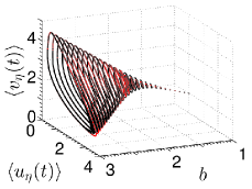
(b)

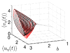
Figure 5: (Color online) The left (right) panel shows the Hopf bifurcation that the stochastic Brusselator averaged orbits exhibit for thermal (multiplicative) noise with constant (linear) diffusion coefficients, $h_{ij}$, as a function of the control parameter $b$ for constant $a=1$. Specifically, the diffusion coefficients are given by $h_{ij}=\delta_{ij}\Gamma$ ($h_{ij}=\delta_{ij}\,x_{j}\,\Gamma$, with $x_{1}=u_{\eta}$ and $x_{2}=v_{\eta}$) with $\Gamma=10^{-2}$. The light (red online) curves correspond to the deterministic orbits and the dark (black online) curves correspond to the noise averaged orbit in each stochastic scenario [additive noise in panel (a) and multiplicative noise in panel (b)] for $100$ noise realisations. For this $\Gamma$, the deterministic and stochastic orbits are very similar, specially for the additive noise scenario.

As it is seen from Fig. 5, the Hopf bifurcation for the Brusselator is conserved in the additive [Fig. 5(a)] and multiplicative [Fig. 5(b)] cases for mild noise intensities ($\Gamma=10^{-2}$). In general, we observe that the effect of increasing the noise strength is to reduce the amplitude of the limit-cycle oscillations in the super-critical regime ($b>b_{c}$), hence, destroying gradually the Hopf bifurcation. Moreover, the multiplicative noise realisations generate an even greater decrease in amplitude. Nevertheless, as it is seen from Fig. 6, both stochastic scenarios maintain the bifurcation type up to noise strengths of $10^{-1}$, where the bifurcation is finally lost.

Besides the determination of the critical noise strength where the Hopf bifurcation is lost, Fig. 6 also shows a somehow universal behaviour of the stochastic system with respect to the deterministic case. In the sub-critical regime, and for parameter values far from the critical point, the orbits quadratic difference scales linearly with the noise intensity ($\Delta^{2}/\Gamma^{2}\sim 10^{-1}$). On the other hand, in the supercritical regime, the orbits quadratic difference collapse under a common curve as a function of the control parameter. To the best of our knowledge, such behaviour has not been accounted in previous works.

(a)

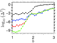
(b)

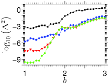
Figure 6: (Color online) The orbits quadratic difference, i.e., the time average quadratic difference between the deterministic and average stochastic orbit ($\Delta^{2}=\frac{1}{T}\sum_{t}\left[\vec{x}(t)-\left\langle\vec{x}_{\eta}(t)\right\rangle\right]^{2}$), for the additive (left panel) and multiplicative (right panel) noisy Brusselator as the control parameter, $b$, is increased for various noise strengths, $\Gamma$. The diffusion coefficients are given by $h_{ij}=\delta_{ij}\Gamma$ for panel (a) [$h_{ij}=\delta_{ij}\,x_{j}\,\Gamma$, with $x_{1}=u_{\eta}$ and $x_{2}=v_{\eta}$, for panel (b)]. The curves correspond to noise intensities of $\Gamma=10^{-1}$ (filled –black online– squares), $10^{-2}$ (filled –blue online– circles), $10^{-3}$ (filled –red online– triangles), and $10^{-4}$ (filled –green online– diamonds).

IV Discussion

In this work we study the Brusselator dynamical behaviour in the absence and presence of random fluctuations and derive some general expressions for generic stochastic systems.

In the non-stochastic dynamics, all main physical properties of the Brusselator, such as the spectral values for the equilibrium states, are found and discussed. The inclusion of thermal and multiplicative noise to the system is first analysed analytically via generic Stochastic Differential Equations. For the thermal noise scenario, expressions for the noise average deviation [Eq. (13)], noise average quadratic deviations [Eq. (14)], variance rate growth [Eq. (16)], and variance asymptotic behaviour [Eq. (18)] are derived.

From our numerical experiments, we conclude that the transition that the Brusselator exhibits from one parameter region, where the chemical concentrations are in a time independent equilibrium state, to another one, where they oscillate in time, is proved to be maintained for moderate values of the noise strength ($<0.1$) in both stochastic scenarios (additive or multiplicative noise). The character of this transition, which is Hopf-like for the deterministic evolution, is still observed in the numerical experiments noise averaged evolutions of the chemical concentrations. Moreover, the analytical expression for the noise averaged orbit [Eq. (13)] and the variance [Eq. (14)] in the case of additive noise, which we derive in a general framework, support these findings.

The expression found for the rate at which the variance grows initially [Eq. (16)], is discussed as the Brusselator’s diffusion processes and correlated to the regular Random Walk. Hence, it is accounted as a Einstein diffusion relationship for the Brusselator. Such analogy is further explored by the derivation of a general expression for the asymptotic value of the variance of the noisy orbits from the fixed-point state [Eq. (18)]. Consequently, the stochastic character that is included into the deterministic Brusselator evolution for the chemical concentrations accounts for the molecular random fluctuations that the real chemical species involved in the reaction exhibit.

References

- (1) S. Strogatz, Sync: The emerging science of spontaneous order (Hyperion, New York, 2003).
- (2) J. D. Murray, Mathematical Biology (Springer, Berlin, 2002).
- (3) G. Nicolis and I. Prigogine, Self-Organization in Non-Equilibrium Systems (Wiley, New York, 1977).
- (4) D. Broomhead, G. McCreadie, and G. Rowlands, Phys. Lett. 84A, 229-231 (1981).
- (5) V.V. Osipov and E.V. Ponizovskaya, Phys. Rev. E 61(4), 4603 (2000).
- (6) K.I. Agladze, V.I. Krinsky, and A.M. Pertsov, Nature 308, 834-835 (1984).
- (7) M. Karplus and G.A. Petsko, Nature 347, 631-639 (1990).
- (8) E. Ziv, I. Nemenman, H.Ch. Wiggins, PLoS ONE 2(10), e1077 (2007).
- (9) R.C. Hilborn, B. Brookshire, J. Mattingly, A. Purushotham, and A. Sharma, PLoS ONE 7(4), e34536 (2012).
- (10) L. Ciandrini, I. Stansfield, and M.C. Romano, PLoS Comput Biol 9(1), e1002866 (2013).
- (11) L.E. Reichl, A Modern Course in Statistical Physics (John Wiley & Sons, 2nd Ed., Canada, 1998).
- (12) J. Guckenheimer and P. Holmes, Nonlinear Oscilations, Dynamical Systems, and Bifurcations of Vector Fields (Springer-Verlag, New York, 1983).
- (13) A. Traulsen, J.Ch. Claussen, and Ch. Hauert, Phys. Rev. Lett. 95, 238701 (2005).
- (14) J.H. Schleimer and M. Stemmler, Phys. Rev. Lett. 103, 248105 (2009).
- (15) A. Melbinger, J. Cremer, and E. Frey, Phys. Rev. Lett. 105, 178101 (2010).
- (16) G. Amselem, M. Theves, A. Bae, E. Bodenschatz, and C. Beta, PLoS ONE 7(5), e37213 (2012).
- (17) F. Duan, F. Chapeau-Blondeau, and D. Abbott, PLoS ONE 9(3), e91345 (2014).
- (18) T. Biancalani, D. Fanelli, and F. Patti, Phys. Rev. E 81, 046215 (2010).
- (19) T. Biancalani, T. Galla, and A.J. McKane, Phys. Rev. E 84, 026201 (2011).
- (20) T. Butler and N. Goldenfeld, Phys. Rev. E 84, 011112 (2011).
- (21) W.H. Press, S.A. Teukolsky, W.T. Vetterling, and B.P. Flannery, Numerical Recipes in Fortran 77: The Art of Scientific Computing (Cambridge University Press, 2nd Ed,1992).
- (22) D.E. Knuth, The art of Computer Programming: Seminumerical Algorithms (Addison-Wesley, Reading, 1969).
- (23) K. Burrage, I. Lenane, and G. Lythe, SIAM J. Sci. Comput. 29, 245-264 (2007).