The theorems of Schottky and Landau for analytic
functions omitting the $\mathbf{n}$–th roots of unity

Abstract. We prove sharp Landau– and Schottky–type theorems for analytic functions which omit the $n$–th roots of unity. The proofs are based on a sharp lower bound for the Poincaré metric of the complex plane punctured at the roots of unity.

1 Introduction

Let ${\mathbb{D}}:=\{z\in{\mathbb{C}}\,:\,|z|<1\}$ denote the open unit disk in the complex plane ${\mathbb{C}}$. In [7] J. Hempel established sharp versions of the classical theorems of Landau [12] and Schottky [20], which are concerned with functions analytic on ${\mathbb{D}}$ that omit the values $0$ and $1$. Related results have been obtained e.g. by Ahlfors [2], Hayman [5] and Jenkins [9].

In [11] Hempel’s work has been extended to meromorphic functions belonging to the classes ${\cal M}_{j,k,l}$, which are defined as follows. Let $j,k,l\geq 2$ be integers (or $=\infty$) such that

$$\frac{1}{j}+\frac{1}{k}+\frac{1}{l}<1\,,$$

and, for any domain $G\subseteq{\mathbb{C}}$, let

$$\begin{array}[]{rl}{\cal M}_{j,k,l}(G):=\{f\text{ meromorphic in }G\text{ s.t.}&\text{\,\,(i) all zeros of }f\text{ have order }\geq j,\\ &\text{\,(ii) all}\text{ zeros}\text{ of }f-1\text{ have order }\geq k,\\ &\hskip 17.07182pt\text{ and }\\ &\text{(iii) all poles of }f\text{ have order }\geq l\}\,.\end{array}$$

Note that ${\cal M}_{\infty,\infty,\infty}({\mathbb{D}})$ consists of all functions analytic in ${\mathbb{D}}$ that omit $0$ and $1$. The motivation for introducing the classes ${\cal M}_{j,k,l}$ comes mainly from Nevanlinna’s celebrated Second Fundamental Theorem which in particular implies that ${\cal M}_{j,k,l}({\mathbb{C}})$ contains only constant functions. The corresponding normality result has been established by Drasin [3], who proved that ${\cal M}_{j,k,l}({\mathbb{D}})$ is a normal family, thereby extending an earlier result of Montel [16, p. 125–126]. Recently, sharp qualitative Landau– and Schottky–type theorems for the classes ${\cal M}_{j,k,l}$ have been obtained in [11].

In the present paper we employ the methods and results of [11] to prove precise Landau– and Schottky–type results for functions analytic in ${\mathbb{D}}$ which omit the $n$–th roots of unity. For any integer $n\geq 1$ we denote by

$$S_{n}=:\{e^{2\pi i\,j/n}\,:\,j=1,\ldots,n\}$$

the set of $n$–th roots of unity. We say a function $f$ analytic in ${\mathbb{D}}$ omits a set $S\subseteq{\mathbb{C}}$ if $f({\mathbb{D}})\cap S=\emptyset$. Further, it will be convenient to make the following formal definition.

Definition 1.1

For each integer $n\geq 2$ let

$$\gamma_{n}=\frac{1}{\lambda_{{\mathbb{C}}\backslash S_{n}}(e^{i\pi/n})}\,,$$

where $\lambda_{{\mathbb{C}}\backslash S_{n}}$ denotes the density of the hyperbolic metric on ${\mathbb{C}}\backslash S_{n}$ with constant curvature $-1$.

For details concerning the hyperbolic metric $\lambda_{{\mathbb{C}}\backslash S_{n}}(z)\,|dz|$ we refer to Section 2.

Now we can state a sharp Landau–type theorem for functions which omit $S_{n}$ for a fixed integer $n\geq 2$.

Theorem 1.1

Fix an integer $n\geq 2$. Let $f(z)=a_{0}+a_{1}z+\ldots$ be an analytic function on ${\mathbb{D}}$ and suppose that $f$ omits $S_{n}$. Then

$$|a_{1}|\leq\begin{cases}2|a_{0}|\sinh\big{(}\mathop{{\rm arcsinh}}\left(\gamma_{n}\right)-\log|a_{0}|\big{)}&\quad\quad\text{ if }\,\,|a_{0}|\leq 1,\\[5.69054pt] 2|a_{0}|\big{(}\gamma_{n}+\log|a_{0}|\big{)}&\quad\quad\text{ if }\,\,|a_{0}|>1\,.\end{cases}$$ (1.1)

Equality occurs in (1.1) if and only if $f$ is a universal covering map onto ${\mathbb{C}}\backslash S_{n}$ with $f(0)^{n}=\nolinebreak-1$.

Here, for $a_{0}=0$ inequality (1.1) is interpreted as

$$|a_{1}|\leq\lim_{a_{0}\to 0}\Big{[}2|a_{0}|\sinh\big{(}\mathop{{\rm arcsinh}}\left(\gamma_{n}\right)-\log|a_{0}|\big{)}\Big{]}=\frac{1+2\gamma_{n}^{2}+2\gamma_{n}\sqrt{1+\gamma_{n}^{2}}}{\gamma_{n}+\sqrt{1+\gamma_{n}^{2}}}\,.$$

Some information about the constants $\gamma_{n}$ can be gleaned. For this, recall that the standard hypergeometric function ${}_{2}F_{1}(a,b,c;z)$ is defined as

$${}_{2}F_{1}(a,b,c;z)=\sum\limits_{k=0}^{\infty}\frac{(a)_{k}(b)_{k}}{(c)_{k}}z^{k}\,,\qquad z\in{\mathbb{D}}\,,$$

where $(a)_{k}:=a(a+1)\cdots(a+k-1)$ is the Pochhammer symbol.

Theorem 1.2

• For every integer $n\geq 2$, the constant $\gamma_{n}$ can be computed:

  $$\begin{array}[]{rcl}\gamma_{n}&=&\displaystyle\frac{2^{\frac{1}{n}}\sin\left(\frac{\pi}{n}\right)\Gamma\left(\frac{1}{n}\right)\Gamma\left(\frac{n-1}{2n}\right)^{2}}{n\,\pi}\,{}_{2}F_{1}\left(\frac{n-1}{2n},\frac{n-1}{2n},1;\frac{1}{2}\right)\,_{2}F_{1}\left(\frac{n-1}{2n},\frac{n-1}{2n},\frac{n-1}{n};\frac{1}{2}\right)\\[11.38109pt] &&\displaystyle-\,\frac{2^{\frac{1}{n}}\pi\tan\left(\frac{\pi}{2n}\right)}{n}\,{}_{2}F_{1}\left(\frac{n-1}{2n},\frac{n-1}{2n},1;\frac{1}{2}\right)^{2}\,.\end{array}$$ (1.2)

• The constants $\gamma_{n}$ are strictly decreasing positive numbers, i.e., $\gamma_{n}>\gamma_{n+1}>0$ for $n=2,3,\ldots$ and $\lim\limits_{n\to\infty}\gamma_{n}=0$.

• For every integer $n\geq 2$:

  $$\gamma_{n}=\dfrac{1}{\min\limits_{|z|=1}\lambda_{{\mathbb{C}}\backslash S_{n}}(z)}\,.$$

Here is a little overview of the first values of the $\gamma_{n}$’s.

$n$	$\gamma_{n}$
2	3.52993
3	1.79372
4	1.22801
5	0.942245
10	0.445789
100	0.0437768
1000	0.00437689

It is perhaps worth making some remarks.

Remark 1.3

Since $(\gamma_{n})$ is a strictly decreasing sequence, the upper bound (1.1) for $|a_{1}|$ provided by Theorem 1.1 is strictly decreasing with respect to $n$. At first sight, this is a surprising fact, because a function which omits $S_{n+1}$ does not necessarily omit $S_{n}$.

Remark 1.4 (The case $\mathbf{n=2}$)

The case $n=2$ of Theorem 1.1 is related to Hempel’s sharp version of Landau’s theorem [7], which says that

$$|b_{1}|\leq 2|b_{0}|\left(\big{|}\log|b_{0}|\big{|}+\frac{\Gamma(\frac{1}{4})^{4}}{4\pi^{2}}\right)$$

for every analytic function $g(z)=b_{0}+b_{1}z+\ldots$ from ${\mathbb{D}}$ into ${\mathbb{C}}\backslash\{0,1\}$. This is equivalent to

$$|a_{1}|\leq 2|a_{0}+1|\left(\left|\log\left|\frac{a_{0}+1}{2}\right|\right|+\frac{\Gamma(\frac{1}{4})^{4}}{4\pi^{2}}\right)$$ (1.3)

for every analytic function $f(z)=a_{0}+a_{1}z+\ldots$ from ${\mathbb{D}}$ into ${\mathbb{C}}\backslash S_{2}$. It can be shown that the estimate (1.1) of Theorem 1.1 is sharper than (1.3) for $a_{0}$ in a neighborhood of the origin or in the right halfplane. On the other hand, (1.3) is better than (1.1) if $a_{0}$ is close to $-1$, see Figure 1.

         

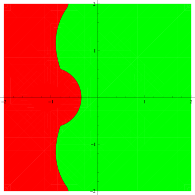
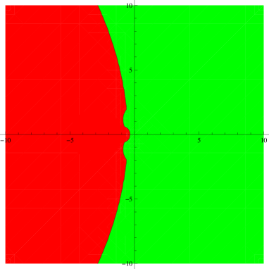
Figure 1: The estimate (1.1) is sharper than (1.3) for $a_{0}$ in the green region and the estimate (1.3) is sharper than (1.1) in the red region.

Remark 1.5 (The case $\mathbf{n\to\infty}$)

In the limit $n\to\infty$, Theorem 1.1 reduces to the well–known Schwarz–Pick lemma. In order to see this, note that in view of Theorem 1.2 (b)

$$\lim\limits_{n\to\infty}\gamma_{n}=0\,.$$

Hence, if a function $f(z)=a_{0}+a_{1}z+\ldots$ analytic in ${\mathbb{D}}$ omits $\partial{\mathbb{D}}=\{z\in{\mathbb{C}}:|z|=1\}$, then letting $n\to\infty$ in estimate (1.1) yields

$$|a_{1}|\leq\begin{cases}\,2|a_{0}|\sinh\left(-\log|a_{0}|\right)=1-|a_{0}|^{2}&\quad\qquad\text{ if }\,\,|a_{0}|\leq 1,\\[5.69054pt] \,2|a_{0}|\log|a_{0}|&\quad\qquad\text{ if }\,\,|a_{0}|>1\,.\end{cases}$$

In particular, if $f$ maps ${\mathbb{D}}$ into ${\mathbb{D}}$, this implies the Schwarz–Pick inequality $|a_{1}|\leq 1-|a_{0}|^{2}$.

We wish to emphasize that Theorem 1.1 might be viewed as interpolation between Landau’s theorem ($n=2$; Remark 1.4) and the Schwarz–Pick lemma ($n=\infty$; Remark 1.5).

The next result provides a sharp Schottky–type bound for analytic functions in ${\mathbb{D}}$ which omit $S_{n}$ for fixed integer $n\geq 2$. As usual $\log^{+}x:=\max\{0,\log x\}$ for every positive real number $x$.

Theorem 1.6

Fix an integer $n\geq 2$. Let $f$ be an analytic function on ${\mathbb{D}}$ and suppose that $f$ omits $S_{n}$. Then for all $z\in{\mathbb{D}}$

$$\log|f(z)|\leq\big{(}\gamma_{n}+\log^{+}|f(0)|\big{)}\frac{1+|z|}{1-|z|}-\gamma_{n}\,.$$ (1.4)

This estimate is sharp in the following sense: if $M>0$ is a constant such that

$$\log|f(z)|\leq\left[M+\log^{+}|f(0)|\right]\frac{1+|z|}{1-|z|}-M$$ (1.5)

holds for all $z\in{\mathbb{D}}$ and all analytic functions $f:{\mathbb{D}}\to{\mathbb{C}}\backslash S_{n}$, then $M\geq\gamma_{n}$.

Estimate (1.4) is rather crude at $z=0$ if $|f(0)|<1$, e.g. if $f(0)=0$. However, in this case one can combine the upper bound (1.4) with Schwarz’s lemma in order to arrive at the following result.

Theorem 1.7 (Schwarz lemma for functions omitting the $\mathbf{n}$–th roots of unity)

Let $n\geq 2$ be an integer and define

$$\begin{array}[]{rcl}R_{n}&=&\displaystyle 1+\gamma_{n}-\sqrt{\gamma_{n}^{2}+2\gamma_{n}}\,.\end{array}$$ (1.6)

Suppose $f$ is an analytic function on ${\mathbb{D}}$ that omits $S_{n}$. If $f(0)=0$, then

$$|f(z)|\leq\frac{1}{R_{n}}\exp\left(\sqrt{\gamma_{n}^{2}+2\gamma_{n}}-\gamma_{n}\right)\,|z|\,,\qquad|z|<R_{n}\,.$$ (1.7)

Theorem 1.7 merits some comment.

Remark 1.8

We note (see Section 3.3) that $(R_{n})$ is a strictly increasing sequence with limit $1$ and

$$\left(\frac{1}{R_{n}}\exp\left(\sqrt{\gamma_{n}^{2}+2\gamma_{n}}-\gamma_{n}\right)\right)$$

forms a strictly decreasing sequence, which converges to $1$ as $n$ tends to $\infty$. Hence, letting $n\to\infty$ Theorem 1.7 reduces to Schwarz’s lemma. Consequently, the estimate (1.7) is asymptotically sharp.

A few examples for $R_{n}$ and $\frac{1}{R_{n}}\exp\left(\sqrt{\gamma_{n}^{2}+2\gamma_{n}}-\gamma_{n}\right)$ are given in the next table.

$n$	$R_{n}$	$\frac{1}{R_{n}}\exp\left(\sqrt{\gamma_{n}^{2}+2\gamma_{n}}-\gamma_{n}\right)$
2	0.111756	21.7516
3	0.185105	12.2035
4	0.237023	9.0483
5	0.277218	7.43155
10	0.401612	4.5297
100	0.744661	1.73354
1000	0.910713	1.20059

We further remark that

$$|f^{\prime}(0)|\leq\frac{1}{R_{n}}\exp\left(\sqrt{\gamma_{n}^{2}+2\gamma_{n}}-\gamma_{n}\ \right)=1+8\frac{\Gamma(5/4)}{\Gamma(3/4)}\frac{1}{\sqrt{n}}+O(1/n)\qquad(n\to\infty)$$

for each $f\in\mathcal{A}_{n}:=\{f:{\mathbb{D}}\to{\mathbb{C}}\backslash S_{n}\text{ holomorphic}\,|\,f(0)=0\}$. However, if $f_{n}\in\mathcal{A}_{n}$ is a universal covering map of ${\mathbb{C}}\backslash S_{n}$, then we get

$$\sup_{f\in\mathcal{A}_{n}}|f^{\prime}(0)|=|f_{n}^{\prime}(0)|=\frac{\Gamma\left(\frac{1}{2}\left(1-\frac{1}{n}\right)\right)^{2}\Gamma\left(\frac{1}{n}\right)}{n\Gamma\left(1-\frac{1}{n}\right)\Gamma\left(\frac{1}{2}\left(1+\frac{1}{n}\right)\right)^{2}}=1+\frac{4\log 2}{n}+O(1/n^{2})\qquad(n\to\infty)\,.$$

This shows that estimate (1.7) is asymptotically sharp only “up to order zero”.

At the end of this introduction we wish to mention that a major motivation for considering holomorphic functions which omit the $n$–th roots of unity has been the beautiful proof of Montel’s fundamental normality criterion based on the Zalcman lemma (see [21]) where holomorphic functions which omit the $n$–th roots of unit play a key role.

In the following section we prove a sharp lower bound for the hyperbolic metric $\lambda_{{\mathbb{C}}\backslash S_{n}}(z)\,|dz|$, see Theorem 2.1. This result is a key ingredient in the proof of Theorem 1.1, but it is of some interest in its own right. The proofs of the results in the Introduction are deferred to Section 3.

2 An explicit sharp lower bound for the hyperbolic metric of the complex plane punctured at the $\mathbf{n}$–roots of unity

Let $U\subseteq{\mathbb{C}}$ be an open set. The quantity $\lambda(z)\,|dz|$ is called a conformal metric on $U$, if $\lambda$ is a strictly positive function on $U$ and $\lambda$ is twice continuously differentiable on $U$, i.e. $\lambda\in C^{2}(U)$. If in addition $\lambda$ satisfies

$$\frac{\Delta\log\lambda(z)}{\lambda(z)^{2}}=1\quad\text{ for all }z\in U,$$

where $\Delta$ is the standard Laplace Operator, then we say $\lambda(z)\,|dz|$ has constant curvature $-1$ on $U$. It is a well-known fact that a hyperbolic domain $\Omega\subset{\mathbb{C}}$, i.e. $\Omega$ has at least two distinct boundary points, carries a unique maximal conformal metric with constant curvature $-1$ (see, for instance, Theorem 13.2 in [6]). This metric is called the hyperbolic metric for $\Omega$ and is denoted by

$$\lambda_{\Omega}(z)\,|dz|\,.$$

In particular,

$$\mu(z)\leq\lambda_{\Omega}(z)\,,\qquad z\in\Omega\,,$$ (2.1)

for every conformal metric $\mu(z)\,|dz|$ on $\Omega$ with constant curvature $-1$.

We now turn to a sharp lower bound for the hyperbolic metric $\lambda_{{\mathbb{C}}\backslash S_{n}}(z)\,|dz|$.

Theorem 2.1

Let $n\geq 2$ be an integer. Then for all $z\in{\mathbb{C}}\backslash S_{n}$,

$$\lambda_{{\mathbb{C}}\backslash S_{n}}(z)\geq\begin{cases}\displaystyle\frac{1}{|z|\sinh\big{(}\mathop{{\rm arcsinh}}\left(\gamma_{n}\right)-\log|z|\big{)}}\qquad\quad&\text{ if }\,|z|\leq 1\,,\\[11.38109pt] \displaystyle\frac{1}{|z|\left(\displaystyle\gamma_{n}+\log|z|\right)}\qquad\quad&\text{ if }\,|z|>1\,.\end{cases}$$ (2.2)

Equality holds in (2.2) if and only if $z^{n}=-1$.

Here, it is understood that

$$\lambda_{{\mathbb{C}}\backslash S_{n}}(0)\geq\lim_{z\to 0}\frac{1}{|z|\sinh\big{(}\mathop{{\rm arcsinh}}\left(\gamma_{n}\right)-\log|z|\big{)}}=\frac{2(\gamma_{n}+\sqrt{1+\gamma_{n}^{2}})}{1+2\gamma_{n}^{2}+2\gamma_{n}\sqrt{1+\gamma_{n}^{2}}}\,.$$

The proof of Theorem 2.1 is based on the theory developed in [11], which deals with conformal metrics with cusps and corners. So let us put together some of the needed details.

Let $G\subseteq{\mathbb{C}}$ be a domain. Suppose first, $p\in G$ and $\lambda(z)\,|dz|$ is a conformal metric on $G\backslash\{p\}$. Then we say $\lambda(z)\,|dz|$ has a corner of order $\alpha<1$ at $p$, if

$$\log\lambda(z)=-\alpha\log|z-p|+O(1)\qquad\text{ as }z\to p\,,$$

and a cusp at $p$, if

$$\log\lambda(z)=-\log|z-p|-\log\left(-\log|z-p|\right)+O(1)\qquad\text{ as }z\to p\,.$$

If, however, $\Delta_{R}:=\{z\in{\mathbb{C}}:|z|>R\}\subseteq G$ for some $R\geq 0$ and $\lambda(z)\,|dz|$ is a conformal metric on $G$, then $\lambda(z)\,|dz|$ has a corner of order $\alpha<1$ at $\infty$, provided

$$\log\lambda(z)=-(2-\alpha)\log|z|+O(1)\qquad\text{ as }z\to\infty\,,$$

and a cusp at $\infty$, if

$$\log\lambda(z)=-\log|z|-\log\left(\log|z|\right)+O(1)\qquad\text{ as }z\to\infty\,.$$

We say a conformal metric $\lambda(z)\,|dz|$ has a singularity of order $\alpha\leq 1$ at $p\in{\mathbb{C}}\cup\{\infty\}$, if either $\lambda(z)\,|dz|$ has a corner of order $\alpha<1$ at $p$ or a cusp at $p$, if $\alpha=1$. Note, that the only isolated singularities of a conformal metric with constant curvature $-1$ are corners and cusps (see [17, 10]).

In particular, the hyperbolic metric $\lambda_{\Omega}(z)\,|dz|$ for a hyperbolic domain $\Omega\subset{\mathbb{C}}$ has a cusp at every isolated boundary point of $\Omega$ and if $\Delta_{R}\subseteq\Omega$ for some $R\geq 0$, then $\lambda_{\Omega}(z)\,|dz|$ has also a cusp at $\infty$, see [6, §18] and [15].

We now record two lemmas about cusps and corners of conformal metrics, which will be needed later. The first lemma gives some information about the remainder function $O(1)$ at a cusp and the second result is a removable singularity theorem.

Lemma 2.2 (cf. Theorem 3.5 in [10])

Let $G\subseteq{\mathbb{C}}$ be a domain.

• If $p\in G$ and $\lambda(z)|dz|$ is a conformal metric with constant curvature $-1$ on $G\backslash\{p\}$ which has a cusp at $p$, then

  $$\lim_{z\to p}\Big{(}\log\lambda(z)+\log|z-p|+\log\left(-\log|z-p|\right)\Big{)}=0\,.$$

• If $\Delta_{R}\subset G$ and $\lambda(z)|dz|$ is a conformal metric with constant curvature $-1$ on $G$ which has a cusp at $\infty$, then

  $$\lim_{z\to\infty}\Big{(}\log\lambda(z)+\log|z|+\log\left(\log|z|\right)\Big{)}=0\,.$$

Lemma 2.3 (cf. Theorem 1.1 in [10])

Let $G\subseteq{\mathbb{C}}$ be a domain, $p\in G$ and suppose $\lambda(z)|dz|$ is a conformal metric with constant curvature $-1$ on $G\backslash\{p\}$ which has a corner of order $\alpha=0$ at $p$. Then the function $\log\lambda$ has a $C^{2}$–extension to $G$. In particular, $\lambda(z)\,|dz|$ is a conformal metric with constant curvature $-1$ on $G$.

It is a well–known fact that for real parameters $\alpha_{1},\alpha_{2},\alpha_{3}\in(0,1]$ which fulfill $\alpha_{1}+\alpha_{2}+\alpha_{3}>2$ there exists a unique conformal metric

$$\lambda_{\alpha_{1},\alpha_{2},\alpha_{3}}(z)\,|dz|\,,\qquad z\in{\mathbb{C}}\backslash\{0,1\}\,,$$

with constant curvature $-1$ on ${\mathbb{C}}\backslash\{0,1\}$ and a singularity of oder $\alpha_{1}$ at $z=0$, $\alpha_{2}$ at $z=1$ and $\alpha_{3}$ at $z=\infty$ such that

$$\mu(z)\leq\lambda_{\alpha_{1},\alpha_{2},\alpha_{3}}(z)\,,\quad z\in{\mathbb{C}}\backslash\{0,1\}\,,$$ (2.3)

for every conformal metric $\mu(z)\,|dz|$ on ${\mathbb{C}}\backslash\{0,1\}$ with constant curvature $-1$ which has a singularity of order $\beta_{1}\leq\alpha_{1}$ at $z=0$, $\beta_{2}\leq\alpha_{2}$ at $z=1$ and $\beta_{3}\leq\alpha_{3}$ at $z=\infty$, see [6, §18–§22]. This metric $\lambda_{\alpha_{1},\alpha_{2},\alpha_{3}}(z)\,|dz|$ is also called the generalized hyperbolic metric on ${\mathbb{C}}\backslash\{0,1\}$ with singularities of order $\alpha_{1}$, $\alpha_{2}$ and $\alpha_{3}$ at $z=0$, $z=1$ and $z=\infty$ respectively.

In the proof of Theorem 2.1, the conformal metric

$$\lambda_{1-1/n,1,1}(w)\,|dw|\,,\qquad w\in{\mathbb{C}}\backslash\{0,1\},$$

where $n\geq 2$ is an integer, provides a key link to $\lambda_{{\mathbb{C}}\backslash S_{n}}(w)\,|dw|$. In order to relate $\lambda_{{\mathbb{C}}\backslash S_{n}}(z)\,|dz|$ with $\lambda_{1-1/n,1,1}(z)\,|dz|$ we use the concept of the pullback of a conformal metric.

Suppose $\lambda(w)\,|dw|$ is a conformal metric on a domain $D\subseteq{\mathbb{C}}$ and $w=f(z)$ is a nonconstant analytic function from a domain $G\subseteq{\mathbb{C}}$ into $D$, then

$$f^{*}\lambda(z)\,|dz|:=\lambda(f(z))\,|f^{\prime}(z)|\,|dz|$$

is a conformal metric on $G\backslash\{z\in G:f^{\prime}(z)=0\}$ and is called the pullback of $\lambda(w)\,|dw|$ under the map $f$. If in addition $\lambda(z)\,|dz|$ has constant curvature $-1$ on $D$, then it is easy to see that $f^{*}\lambda(z)\,|dz|$ has constant curvature $-1$ on $G\backslash\{z\in G:f^{\prime}(z)=0\}$.

Now, roughly speaking, the hyperbolic metric $\lambda_{{\mathbb{C}}\backslash S_{n}}(w)\,|dw|$ is the pullback of the generalized hyperbolic metric $\lambda_{1-1/n,1,1}(z)\,|dz|$ under the map $w=z^{n}$. This is the content of our next theorem.

Theorem 2.4

Let $n\geq 2$ be an integer. Then

$$\lambda_{{\mathbb{C}}\backslash S_{n}}(z)=n|z|^{n-1}\lambda_{1-1/n,1,1}(z^{n})\,$$

for every $z\in{\mathbb{C}}\backslash(S_{n}\cup\{0\})$ and

$$\lambda_{{\mathbb{C}}\backslash S_{n}}(0)=\lim_{z\to 0}n|z|^{n-1}\lambda_{1-1/n,1,1}(z^{n})\,.$$

Proof. Let $f:{\mathbb{C}}\to{\mathbb{C}}$, $f(z)=z^{n}$. Note that $f$ maps ${\mathbb{C}}\backslash(S_{n}\cup\{0\})$ onto ${\mathbb{C}}\backslash\{0,1\}$. Thus

$$\lambda_{n}(z)\,|dz|:=f^{*}\lambda_{1-1/n,1,1}(z)\,|dz|=n|z|^{n-1}\lambda_{1-1/n,1,1}(z^{n})\,|dz|\,,\qquad z\in{\mathbb{C}}\backslash(S_{n}\cup\{0\})\,,$$

defines a conformal metric on ${\mathbb{C}}\backslash(S_{n}\cup\{0\})$ with constant curvature $-1$.

Our objective is to show that $\lambda_{n}(z)\,|dz|$ extends to be a conformal metric with constant curvature $-1$ on all of ${\mathbb{C}}\backslash S_{n}$ and

$$\lambda_{n}(z)\,|dz|=\lambda_{{\mathbb{C}}\backslash S_{n}}(z)\,|dz|\quad\text{ on }\,{\mathbb{C}}\backslash S_{n}\,.$$

We first determine the type of singularities of $\lambda_{n}(z)\,|dz|$ at the points $p\in S_{n}\cup\{0,\infty\}$. As $\lambda_{1-1/n,1,1}(z)\,|dz|$ has a cusp at $p=1$, it follows that $\lambda_{n}(z)\,|dz|$ has a cusp at every point $p\in S_{n}$. Similarly, the cusp of $\lambda_{1-1/n,1,1}(z)\,|dz|$ at $p=\infty$ results in a cusp of $\lambda_{n}(z)\,|dz|$ at $p=0$. Now, since $\lambda_{1-1/n,1,1}(z)\,|dz|$ has a corner of order $1-1/n$ at $p=0$, we see that $\lambda_{n}(z)\,|dz|$ is bounded at $p=0$, i.e. $\lambda_{n}(z)\,|dz|$ has a corner of order $\alpha=0$ at $p=0$. By appeal to Lemma 2.3, $\lambda_{n}(z)\,|dz|$ is a conformal metric on ${\mathbb{C}}\backslash S_{n}$ with constant curvature $-1$.

In summary, $\lambda_{n}(z)\,|dz|$ is a conformal metric with constant curvature $-1$ on ${\mathbb{C}}\backslash S_{n}$ which has a cusp at each point $p\in S_{n}\cup\{\infty\}$.

It follows that $\lambda_{n}(z)\leq\lambda_{{\mathbb{C}}\backslash S_{n}}(z)$ for $z\in{\mathbb{C}}\backslash S_{n}$, because $\lambda_{{\mathbb{C}}\backslash S_{n}}(z)\,|dz|$ is the hyperbolic metric on ${\mathbb{C}}\backslash S_{n}$, see (2.1). We next consider on ${\mathbb{C}}\backslash S_{n}$ the nonnegative function

$$s(z)=\log\left(\frac{\lambda_{{\mathbb{C}}\backslash S_{n}}(z)}{\lambda_{n}(z)}\right)\,,\qquad z\in{\mathbb{C}}\backslash S_{n}\,.$$

Then, $s$ is subharmonic on ${\mathbb{C}}\backslash S_{n}$, since

$$\Delta s(z)=\Delta\log\lambda_{{\mathbb{C}}\backslash S_{n}}(z)-\Delta\log\lambda_{n}(z)=\lambda_{{\mathbb{C}}\backslash S_{n}}(z)^{2}-\lambda_{n}(z)^{2}\geq 0\,,\qquad z\in{\mathbb{C}}\backslash S_{n}\,,$$

which is an immediate consequence of the fact that $\lambda_{n}(z)\,|dz|$ and $\lambda_{{\mathbb{C}}\backslash S_{n}}(z)\,|dz|$ have constant curvature $-1$ on ${\mathbb{C}}\backslash S_{n}$. Bearing in mind that both $\lambda_{n}(z)\,|dz|$ and $\lambda_{{\mathbb{C}}\backslash S_{n}}(z)\,|dz|$ have a cusp at each point $p\in S_{n}\cup\{\infty\}$, we conclude with the help of Lemma 2.2 that

$$\lim_{z\to p}s(z)=0\quad\text{ for each }\,p\in S_{n}\qquad\text{and}\qquad\lim_{z\to\infty}s(z)=0\,.$$

Thus, the maximum principle for subharmonic functions (see e.g. Corollary 2.3.3 in [18]) implies $s(z)\leq 0$ for all $z\in{\mathbb{C}}\backslash S_{n}$. Consequently, $s\equiv 0$ on ${\mathbb{C}}\backslash S_{n}$. This gives the desired result

$$\lambda_{n}(z)\,|dz|=\lambda_{{\mathbb{C}}\backslash S_{n}}(z)\,|dz|\,\text{ for }\,z\in{\mathbb{C}}\backslash S_{n}\quad\text{ and }\quad\lambda_{{\mathbb{C}}\backslash S_{n}}(0)=\lim_{z\to 0}\lambda_{n}(z)\,.$$

m $\blacksquare$

Now, Theorem 2.4 enables us to prove Theorem 2.1 by applying the following sharp lower bound for the generalized hyperbolic metric $\lambda_{1-1/n,1,1}(z)\,|dz|$.

Theorem 2.5

Let $n\geq 2$ be an integer. Then for all $w\in{\mathbb{C}}\backslash\{0,1\}$,

$$\lambda_{1-1/n,1,1}(w)\geq\begin{cases}\displaystyle\frac{1}{n|w|\sinh\left[\mathop{{\rm arcsinh}}\left(\displaystyle\frac{1}{n\,\lambda_{1-1/n,1,1}(-1)}\right)-\frac{1}{n}\log|w|\right]}&\qquad\quad\text{ if }\,\,|w|\leq 1\,,\\ &\phantom{\text{ if }}\\ \displaystyle\frac{1}{|w|\left(\displaystyle\frac{1}{\lambda_{1-1/n,1,1}(-1)}+\log|w|\right)}&\qquad\quad\text{ if }\,\,|w|>1\,,\end{cases}$$

with equality if and only if $w=-1$.

Proof. Theorem 2.5 can be obtained from Theorem 2.2 in [11]. In fact, Theorem 2.2 in [11] provides a sharp lower bound for the generalized hyperbolic metric $\lambda_{\alpha_{1},\alpha_{2},\alpha_{3}}(z)\,|dz|$, when $\alpha_{1},\alpha_{2},\alpha_{3}\in(0,1]$ and $\alpha_{1}+\alpha_{2}+\alpha_{3}>2$. Choosing $\alpha_{1}=1-1/n$ and letting $\alpha_{2}\nearrow 1$ and $\alpha_{3}\nearrow 1$ gives Theorem 2.5. $\blacksquare$

Before passing to the proof of Theorem 2.1 let us recall an important result about conformal metrics.

Lemma 2.6 (Theorem 7.1 in [6])

Let $G\subseteq{\mathbb{C}}$ be a domain, $\lambda(z)\,|dz|$ a conformal metric with constant curvature $-1$ on $G$ and let $\mu$ be a nonnegative on $G$ function such that $\mu(z)\,|dz|$ is a conformal metric on $\{z\in G:\mu(z)>0\}$ with constant curvature $-1$. Suppose $\mu(z)\leq\lambda(z)$ for all $z\in G$. Then either $\mu<\lambda$ on $G$ or else $\mu\equiv\lambda$ on $G$.

Proof of Theorem 2.1. By Theorem 2.4 we see that

$$\frac{1}{n\lambda_{1-1/n,1,1}(-1)}=\frac{1}{\lambda_{{\mathbb{C}}\backslash S_{n}}(e^{i\pi/n})}=\gamma_{n}\,.$$ (2.4)

Now combining Theorem 2.4 and Theorem 2.5 gives inequality (2.2).

It remains to show that equality occurs in (2.2) if and only if $z^{n}=-1$. This is clear if $z\not=0$ in view of Theorem 2.4 and the case of equality of Theorem 2.5. Therefore we need only show that for $z=0$ strict inequality holds in (2.2), i.e.,

$$\lambda_{{\mathbb{C}}\backslash S_{n}}(0)>\lim_{z\to 0}\frac{1}{|z|\sinh\left(\mathop{{\rm arcsinh}}\left(\displaystyle\gamma_{n}\right)-\log|z|\right)}=\frac{2(\gamma_{n}+\sqrt{1+\gamma_{n}^{2}})}{1+2\gamma_{n}^{2}+2\gamma_{n}\sqrt{1+\gamma_{n}^{2}}}\,.$$

For this we define $\mu$ on ${\mathbb{D}}$ by

$$\mu(z)=\begin{cases}\dfrac{2(\gamma_{n}+\sqrt{1+\gamma_{n}^{2}})}{1+2\gamma_{n}^{2}+2\gamma_{n}\sqrt{1+\gamma_{n}^{2}}}\qquad\quad&\text{ if }\,\,z=0,\\[17.07164pt] \dfrac{1}{|z|\sinh\left(\mathop{{\rm arcsinh}}(\gamma_{n})-\log|z|\right)}\qquad\quad&\text{ if }\,\,z\in{\mathbb{D}}\backslash\{0\}\,.\end{cases}$$

Since we have already observed that strict inequality occurs in (2.2) for every $z\in{\mathbb{C}}$ with $z\not=0$ and $z^{n}=-1$, respectively, we have in particular

$$\mu(z)<\lambda_{{\mathbb{C}}\backslash S_{n}}(z)\quad\text{ for all }z\in{\mathbb{D}}\backslash\{0\}\,.$$ (2.5)

Now, it is easily checked that $\mu(z)\,|dz|$ is a conformal metric with constant curvature $-1$ on ${\mathbb{D}}\backslash\{0\}$. Since $\mu$ is continuous at $z=0$ and $\mu(0)>0$, Lemma 2.3 tells us that $\mu(z)\,|dz|$ is a conformal metric with constant curvature $-1$ on the entire unit disk ${\mathbb{D}}$, so $\mu(z)\leq\lambda_{{\mathbb{C}}\backslash S_{n}}(z)$ for all $z\in{\mathbb{D}}$ because of (2.5). We are now in a position to apply Lemma 2.6 for $G={\mathbb{D}}$, and obtain, using again (2.5), that $\mu(z)<\lambda_{{\mathbb{C}}\backslash S_{n}}(z)$ for all $z\in{\mathbb{D}}$. This completes the proof. $\blacksquare$

3 Proofs

3.1 Proofs of Theorem 1.1 and Theorem 1.2

Before proving Theorem 1.1 we digress to recall the Ahlfors–Schwarz lemma.

Lemma 3.1 (cf. [2] and §25 in [6])

Let $G\subset{\mathbb{C}}$ be a hyperbolic domain, suppose that $\lambda(z)\,|dz|$ is a conformal metric with constant curvature $-1$ on $G$, and let $f:{\mathbb{D}}\to G$ be a nonconstant analytic function. Then

$$f^{*}\lambda(z)\leq\lambda_{{\mathbb{D}}}(z)\,,\qquad z\in{\mathbb{D}}\,,$$ (3.1)

where $\lambda_{{\mathbb{D}}}(z)\,|dz|=\dfrac{2}{1-|z|^{2}}\,|dz|$ is the hyperbolic metric for ${\mathbb{D}}$.

Equality occurs in (3.1) if and only if $f:{\mathbb{D}}\to G$ is a universal covering map and $\lambda(z)\,|dz|=\lambda_{G}(z)\,|dz|$.

Proof of Theorem 1.1. Let $f:{\mathbb{D}}\to{\mathbb{C}}\backslash S_{n}$ be analytic and nonconstant. Then by Lemma 3.1

$$f^{*}\lambda_{{\mathbb{C}}\backslash S_{n}}(z)=\lambda_{{\mathbb{C}}\backslash S_{n}}(f(z))\,|f^{\prime}(z)|\leq\frac{2}{1-|z|^{2}}\,,\qquad z\in{\mathbb{D}}\,.$$ (3.2)

Thus (3.2) together with Theorem 2.1 implies

$$\frac{2}{1-|z|^{2}}\geq\begin{cases}\displaystyle\frac{|f^{\prime}(z)|}{|f(z)|\sinh\big{(}\mathop{{\rm arcsinh}}(\gamma_{n})-\log|f(z)|\big{)}}&\quad\quad\text{ if }\,\,|f(z)|\leq 1\,,\\[17.07164pt] \displaystyle\frac{|f^{\prime}(z)|}{|f(z)|\left(\gamma_{n}+\log|f(z)|\right)}&\quad\quad\text{ if }\,\,|f(z)|>1\,.\end{cases}$$ (3.3)

As before

$$\frac{|f^{\prime}(z)|}{|f(z)|\sinh\big{(}\mathop{{\rm arcsinh}}(\gamma_{n})-\log|f(z)|\big{)}}$$

should be interpreted to be

$$\lim_{f(z)\to 0}\frac{|f^{\prime}(z)|}{|f(z)|\sinh\big{(}\mathop{{\rm arcsinh}}(\gamma_{n})-\log|f(z)|\big{)}}$$

if $f(z)=0$.

To obtain (1.1) we just insert $z=0$ into (3.3).

We now turn to the case of equality. Note that equality holds in (1.1) if and only if equality occurs in (3.3) for $z=0$. In view of Theorem 2.1 and (3.2) this is the case if and only if

$$\lambda_{{\mathbb{C}}\backslash S_{n}}(f(0))|f^{\prime}(0)|=\lambda_{{\mathbb{D}}}(0)\quad\text{ and }\quad f(0)^{n}=-1\,.$$

Hence, by Lemma 3.1 (case of equality) we see that equality occurs in (1.1) if and only if $f:\nolinebreak{\mathbb{D}}\to{\mathbb{C}}\backslash S_{n}$ is a universal covering with $f(0)^{n}=-1$. $\blacksquare$

We next turn to the proof of Theorem 1.2. In order to determine the value of the constant $\gamma_{n}$, we will make use of the following explicit formula for $\lambda_{1-1/n,1,1}(z)\,|dz|$. For this it is convenient to define

$$\varphi_{1}(z):=_{2}\!\!F_{1}\left(\frac{n-1}{2n},\frac{n-1}{2n},\frac{n-1}{n};z\right)\quad\text{and}\quad\varphi_{2}(z):=_{2}\!\!F_{1}\left(\frac{n-1}{2n},\frac{n-1}{2n},1;1-z\right)\,.$$

Note that $\varphi_{1}$ has an analytic continuation to ${\mathbb{C}}\backslash[1,+\infty)$ and $\varphi_{2}$ has an analytic continuation to ${\mathbb{C}}\backslash(-\infty,0]$.

Theorem 3.2

Let $n\geq 2$ be an integer. Then for $z\in{\mathbb{C}}\backslash\{0,1\}$

$$\lambda_{1-1/n,1,1}(z)=\frac{1}{|z|^{1-1/n}|1-z|}\,\,\frac{1}{\frac{K_{2}}{2K_{3}}\,\,|\varphi_{2}(z)|^{2}+\frac{1}{K_{3}}\mathop{{\rm Re}}\Big{(}\varphi_{1}(z)\varphi_{2}(\overline{z})\Big{)}}\,,$$ (3.4)

where

$$K_{2}:=-\frac{\Gamma\left(\frac{n+1}{2n}\right)^{2}}{\Gamma\left(\frac{1}{n}\right)}\quad\text{ and }\quad K_{3}:=\frac{\Gamma\left(\frac{n-1}{n}\right)}{\Gamma\left(\frac{n-1}{2n}\right)^{2}}\,.$$

Here, for $x\in(1,\infty)$ the right–hand side of equation (3.4) must be interpreted to mean

$$\lim_{z\to x}\frac{1}{|z|^{1-1/n}|1-z|}\,\,\frac{1}{\frac{K_{2}}{2K_{3}}\,\,|\varphi_{2}(z)|^{2}+\frac{1}{K_{3}}\mathop{{\rm Re}}\Big{(}\varphi_{1}(z)\varphi_{2}(\overline{z})\Big{)}}\,.$$

Proof. We note that Theorem 2.1 in [11] displays a formula for the generalized hyperbolic metric $\lambda_{\alpha_{1},\alpha_{2},\alpha_{3}}(z)\,|dz|$ for $0<\alpha_{1},\alpha_{2}<1$, $0<\alpha_{3}\leq 1$ and $\alpha_{1}+\alpha_{2}+\alpha_{3}>2$ in terms of the functions $\varphi_{1}$ and $\varphi_{2}$. Now choosing in this particular theorem $\alpha_{1}=1-1/n$, $\alpha_{3}=1$ and letting $\alpha_{2}\nearrow 1$ yields (3.4). $\blacksquare$

It is convenient to record different representations for the constants $K_{3}$ and $K_{2}/K_{3}$ for later reference.

Using the well–known reflection formula

$$\Gamma(z)\,\Gamma(1-z)=\frac{\pi}{\sin(\pi z)}\,,\qquad z\in{\mathbb{C}}\backslash\mathbb{Z}\,,$$ (3.5)

(cf. [1, p. 77]), we get

$$K_{3}=\frac{\pi}{\sin\left(\frac{\pi}{n}\right)}\,\frac{1}{\Gamma\left(\frac{1}{n}\right)\,\Gamma\left(\frac{n-1}{2n}\right)^{2}}$$ (3.6)

and

$$\begin{split}\frac{K_{2}}{K_{3}}&=-\frac{\Gamma\left(\frac{n+1}{2n}\right)^{2}}{\Gamma\left(\frac{1}{n}\right)}\,\frac{\sin\left(\frac{\pi}{n}\right)}{\pi}\,\,\Gamma\left(\frac{1}{n}\right)\,\,\Gamma\left(\frac{n-1}{2n}\right)^{2}=-\frac{\sin(\frac{\pi}{n})}{\pi}\,\,\Gamma\left(\frac{n-1}{2n}\right)^{2}\,\,\Gamma\left(\frac{n+1}{2n}\right)^{2}\\[5.69054pt] &=-\frac{\sin\left(\frac{\pi}{n}\right)}{\pi}\,\,\frac{\pi^{2}}{\left(\sin\left(\frac{\pi(n-1)}{2n}\right)\right)^{2}}=-2\pi\tan\left(\frac{\pi}{2n}\right)\,.\end{split}$$ (3.7)

Proof of Theorem 1.2.

Recall that

$$\gamma_{n}=\frac{1}{n\lambda_{1-1/n,1,1}(-1)}\,,$$

see (2.4).

• To compute $\gamma_{n}$ we consider the Möbius transformation $T(z)=z/(z-1)$, which fixes $z=0$ and interchanges $z=1$ with $z=\infty$. Note that $\mu(z)\,|dz|:=T^{*}\lambda_{1-1/n,1,1}(z)\,|dz|$ is a conformal metric on ${\mathbb{C}}\backslash\{0,1\}$ with constant curvature $-1$ and a corner of order $1-1/n$ at $z=0$ and a cusp at $z=1$ and $z=\infty$. Thus

  $$\mu(z)\leq\lambda_{1-1/n,1,1}(z)\,,\qquad z\in{\mathbb{C}}\backslash\{0,1\}\,,$$

  by (2.3). Since $T\circ T=\text{Id}$, we observe that $T^{*}\mu(z)\,|dz|=\lambda_{1-1/n,1,1}(z)\,|dz|$ and the latter inequality implies

  $$\lambda_{1-1/n,1,1}(z)\leq\mu(z)\,,\qquad z\in{\mathbb{C}}\backslash\{0,1\}\,.$$

  Consequently,

  $$\lambda_{1-1/n,1,1}(z)=\lambda_{1-1/n,1,1}(T(z))|T^{\prime}(z)|\,,\qquad z\in{\mathbb{C}}\backslash\{0,1\}\,.$$

  Thus we get

  $$\lambda_{1-1/n,1,1}(-1)=\frac{\lambda_{1-1/n,1,1}(1/2)}{4}\,.$$

  Inserting now $z=1/2$ into (3.4) and using (3.6) and (3.7) gives the claimed expression (1.2) for $\gamma_{n}$.

• By (2.3) we have, for all integers $m>n\geq 2$,

  $$\lambda_{1-1/n,1,1}(w)\leq\lambda_{1-1/m,1,1}(w)\,,\qquad w\in{\mathbb{C}}\backslash\{0,1\}\,.$$

  This shows that

  $$0<\gamma_{n}=\frac{1}{n\lambda_{1-1/n,1,1}(-1)}<\frac{1}{m\lambda_{1-1/n,1,1}(-1)}=\gamma_{m}$$

  for $m>n\geq 2$.

  To verify $\lim_{n\to\infty}\gamma_{n}=0$ we consider the sequence

  $$(n\gamma_{n})=\left(\frac{1}{\lambda_{1-1/n,1,1}(-1)}\right)\,.$$

  Since

  $$\lim_{n\to\infty}\lambda_{1-1/n,1,1}(-1)=\lambda_{1,1,1}(-1)=\lambda_{{\mathbb{C}}\backslash\{0,1\}}(-1)$$

  and

  $$\lambda_{{\mathbb{C}}\backslash\{0,1\}}(-1)=\frac{4\pi^{2}}{\Gamma(1/4)^{4}}\,,$$

  see [7], we get

  $$\lim_{n\to\infty}n\gamma_{n}=\frac{\Gamma(1/4)^{4}}{4\pi^{2}}\quad\text{ and }\quad\lim_{n\to\infty}\gamma_{n}=0\,.$$

• It is a known fact, that

  $$\lambda_{1-1/n,1,1}(-1)=\min_{|z|=1}\lambda_{1-1/n,1,1}(z)\,,$$

  see, for instance, Theorem 4.10 in [11]. Thus Theorem 2.4 implies

$$\min\limits_{|z|=1}\lambda_{{\mathbb{C}}\backslash S_{n}}(z)=\min_{|z|=1}n\lambda_{1-1/n,1,1}(z^{n})=n\lambda_{1-1/n,1,1}(-1)=\lambda_{{\mathbb{C}}\backslash S_{n}}(e^{i\pi/n})\,.$$

m $\blacksquare$

3.2 Proof of Theorem 1.6

Proof of Theorem 1.6. To prove (1.4) we proceed exactly as in the proof of Theorem 1 in [13] (see also the proof Theorem 2.8 in [11]). Here are the details. Note that (1.4) is true for $z=0$ and $|f(z)|<1$. So pick a point $z\in{\mathbb{D}}\backslash\{0\}$ such that $|f(z)|>1$. Consider the curve $\gamma(t):=f(t\eta)$ for $t\in[0,|z|]$, where $\eta:=z/|z|$. If $\gamma$ lies completely outside $\overline{{\mathbb{D}}}$, then by (3.3)

$$\frac{|f^{\prime}(t\eta)|}{|f(t\eta)|\left(\gamma_{n}+\log|f(t\eta)|\right)}\leq\frac{2}{1-t^{2}}\,,\qquad t\in[0,|z|]\,.$$ (3.8)

Using

$$\frac{d}{dt}\left(|f(t\eta)|\right)\leq|f^{\prime}(t\eta)|\,,$$

we obtain

$$\log\left(\frac{\gamma_{n}+\log|f(z)|}{\gamma_{n}+\log|f(0)|}\right)=\int\limits_{0}^{|z|}\frac{\frac{d}{dt}\left(|f(t\eta)|\right)}{|f(t\eta)(\gamma_{n}+\log|f(t\eta)|)}\,dt\leq\int\limits_{0}^{|z|}\frac{2}{1-t^{2}}\,dt=\log\frac{1+|z|}{1-|z|}\,,$$

which leads to the desired estimate (1.4).

If $\gamma$ does not completely lie outside $\overline{{\mathbb{D}}}$ we use an argument similar to the one above. Let $\gamma(t^{*})$ be the “last” point of $\gamma(t)$ which lies inside $\overline{{\mathbb{D}}}$. Now integrating (3.8) just from $t^{*}$ to $|z|$ yields

$$\log|f(z)|\leq\gamma_{n}\frac{1+|z|}{1-|z|}-\gamma_{n}\,,$$

which is stronger than (1.4).

Now suppose that (1.5) holds for each analytic map $f$ from ${\mathbb{D}}$ to ${\mathbb{C}}\backslash S_{n}$. Let $\varphi:{\mathbb{D}}\to{\mathbb{C}}\backslash S_{n}$ denote a universal covering map with $\varphi(0)^{n}=-1$. Then it follows from (1.5) that

$$\log|\varphi(z)|\leq 2M\frac{|z|}{1-|z|}\qquad\text{ for all }z\in{\mathbb{D}}\,.$$

We further note that $|\varphi(0)|=1$ and hence there exists a disk ${\mathbb{D}}_{r}:=\{z\in{\mathbb{C}}:|z|<r\}$, $0<r<1$, such that $\varphi(z)\not=0$ for all $z\in{\mathbb{D}}_{r}$.

Choose $\eta\in\partial{\mathbb{D}}$ such that

$$\eta\frac{\varphi^{\prime}(0)}{\varphi(0)}=\left|\frac{\varphi^{\prime}(0)}{\varphi(0)}\right|=|\varphi^{\prime}(0)|$$

and define

$$h(t)=\log|\varphi(\eta t)|\,,\qquad t\in(-r,r)\,.$$

Since $h(0)=0$ we conclude

$$\frac{h(t)-h(0)}{t}\leq 2M\frac{1}{1-t}\,.$$

Letting $t\to 0$, we obtain $h^{\prime}(0)\leq 2M$. On the other hand a simple computation gives

$$h^{\prime}(0)=\mathop{{\rm Re}}\left(\eta\frac{\varphi^{\prime}(0)}{\varphi(0)}\right)=|\varphi^{\prime}(0)|\,.$$

As $\varphi$ is a universal covering map of ${\mathbb{C}}\backslash S_{n}$ with $\varphi(0)^{n}=-1$ Theorem 1.1 shows $|\varphi^{\prime}(0)|=2\gamma_{n}$. Putting these facts together, we see that $\gamma_{n}\leq M$. $\blacksquare$

3.3 Proofs of Theorem 1.7 and Remark 1.8

Proof of Theorem 1.7. Choose $R\in(0,1)$. Since $f(0)=0$, estimate (1.4) implies

$$|f(z)|\leq\exp\left(2\gamma_{n}\frac{|z|}{1-|z|}\right)\leq\exp\left(2\gamma_{n}\frac{R}{1-R}\right)$$

for $z\in{\mathbb{D}}_{R}:=\{z\in{\mathbb{C}}:|z|<R\}$. We use $f(0)=0$ once more to apply the Schwarz’ lemma for the disk ${\mathbb{D}}_{R}$ and obtain

$$|f(z)|\leq\frac{1}{R}\exp\left(2\gamma_{n}\frac{R}{1-R}\right)\,|z|\,,\qquad z\in{\mathbb{D}}_{R}\,.$$ (3.9)

We next consider the function

$$R\mapsto\frac{1}{R}\exp\left(2\gamma_{n}\frac{R}{1-R}\right)\,,\qquad R\in(0,1)\,.$$

It is easy to check that this function attains its minimal value on $(0,1)$ and there is exactly one such point. Call it $R_{n}$. Then a straightforward computation gives formula (1.6) for $R_{n}$. Inserting (1.6) into (3.9) leads to (1.7). $\blacksquare$

Proof of Remark 1.8. First, $(R_{n})$ is a strictly increasing sequence which tends to the limit $1$ because the function $x\mapsto 1+x-\sqrt{x^{2}+2x}$ is strictly decreasing on $[0,\infty)$ and the sequence $(\gamma_{n})$ is strictly decreasing with limit $0$. Once again, since $(\gamma_{n})$ is strictly decreasing, the expression

$$\frac{1}{R}\exp\left(2\gamma_{n}\,\frac{R}{1-R}\right)\,,\qquad R\in(0,1)\,,$$

is strictly decreasing with respect to $n$, so its minimal value

$$\frac{1}{R_{n}}\exp\left(2\gamma_{n}\frac{R_{n}}{1-R_{n}}\right)=\frac{1}{R_{n}}\exp\left(\sqrt{\gamma_{n}^{2}+\gamma_{n}}-\gamma_{n}\right)$$

is also strictly decreasing with respect to $n$ (see the proof of Theorem 1.7).

Consequently,

$$\left(\frac{1}{R_{n}}\exp\left(\sqrt{\gamma_{n}^{2}+\gamma_{n}}-\gamma_{n}\right)\right)$$

forms a strictly decreasing sequence with limit $1$.

Now, let $f\in\mathcal{A}_{n}$. Then inequality (1.7) implies

$$|f^{\prime}(0)|\leq\frac{1}{R_{n}}\exp\left(\sqrt{\gamma_{n}^{2}+2\gamma_{n}}-\gamma_{n}\ \right)\,.$$

A straightforward but lengthy calculation, using Theorem 1.2 (a), gives

$$|f^{\prime}(0)|\leq\frac{1}{R_{n}}\exp\left(\sqrt{\gamma_{n}^{2}+2\gamma_{n}}-\gamma_{n}\ \right)=1+8\frac{\Gamma(5/4)}{\Gamma(3/4)}\frac{1}{\sqrt{n}}+O(1/n)\qquad(n\to\infty)\,.$$

If $f_{n}\in\mathcal{A}_{n}$ is a universal covering map of ${\mathbb{C}}\backslash S_{n}$, then $f_{n}^{*}\lambda_{{\mathbb{C}}\backslash S_{n}}(z)\,|dz|=\lambda_{{\mathbb{D}}}(z)\,|dz|$. Therefore,

$$|f_{n}^{\prime}(0)|=\frac{2}{\lambda_{{\mathbb{C}}\backslash S_{n}}(0)}=\lim\limits_{z\to 0}\frac{2}{n|z|^{n-1}\lambda_{1-1/n,1,1}(z^{n})}$$

by Theorem 2.4. Combining this with Theorem 3.2 and (3.6) as well as (3.7) we get

$$\begin{split}|f_{n}^{\prime}(0)|=\frac{1}{n}&\left(-\frac{\sin\left(\frac{\pi}{n}\right)}{\pi}\,\,\Gamma\left(\frac{n-1}{2n}\right)^{2}\Gamma\left(\frac{n+1}{2n}\right)^{2}\,\,_{2}F_{1}\left(\frac{n-1}{2n},\frac{n-1}{2n},1;1\right)^{2}\right.\\[5.69054pt] &\left.\quad+\,2\,\frac{\sin\left(\frac{\pi}{n}\right)}{\pi}\,\,\Gamma\left(\frac{n-1}{2n}\right)^{2}\Gamma\left(\frac{1}{n}\right)\,\,_{2}F_{1}\left(\frac{n-1}{2n},\frac{n-1}{2n},1;1\right)\right)\,.\end{split}$$

Because of Gauss’s theorem

$${}_{2}F_{1}(a,b,c;1)=\frac{\Gamma(c)\Gamma(c-a-b)}{\Gamma(c-a)\Gamma(c-b)}\quad\text{ for }\quad\mathop{{\rm Re}}(c)>\mathop{{\rm Re}}(a+b),\,\,c\not=0,-1,-2,\ldots\,,$$

(see [1, p. 213]), we get

$$|f_{n}^{\prime}(0)|=\frac{\sin\left(\frac{\pi}{n}\right)\Gamma\left(\frac{1}{n}\right)^{2}\Gamma\left(\frac{n-1}{2n}\right)^{2}}{\pi n\Gamma\left(\frac{n+1}{2n}\right)^{2}}\,.$$

This simplifies, using the reflection formula (3.5), to

$$|f_{n}^{\prime}(0)|=\frac{\Gamma\left(\frac{1}{2}\left(1-\frac{1}{n}\right)\right)^{2}\Gamma\left(\frac{1}{n}\right)}{n\Gamma\left(1-\frac{1}{n}\right)\Gamma\left(\frac{1}{2}\left(1+\frac{1}{n}\right)\right)^{2}}\,.$$

Using the well–known Taylor series expansion

$$1/\Gamma(z)=z+\gamma z^{2}+\cdots$$

at $z=0$, where $\gamma$ is the Euler–Mascheroni constant, (cf. [1, p. 76/77]), one readily verifies that

$$\frac{\Gamma\left(\frac{1}{2}\left(1-\frac{1}{n}\right)\right)^{2}\Gamma\left(\frac{1}{n}\right)}{n\Gamma\left(1-\frac{1}{n}\right)\Gamma\left(\frac{1}{2}\left(1+\frac{1}{n}\right)\right)^{2}}=1+\frac{4\log 2}{n}+O(1/n^{2})\qquad(n\to\infty)\,.$$

The proof of Remark 1.8 is now complete. $\blacksquare$

Figure 2: The hyperbolic density $\lambda_{{\mathbb{C}}\backslash S_{n}}$ for $n=70$

Daniela Kraus
Department of Mathematics
University of Würzburg
Emil Fischer Straße 40
97074 Würzburg
dakraus@mathematik.uni-wuerzburg.de
Phone: +49 931 318 5028

Oliver Roth
Department of Mathematics
University of Würzburg
Emil Fischer Straße 40
97074 Würzburg
roth@mathematik.uni-wuerzburg.de
Phone: +49 931 318 4974

References

- [1] M. Abramowitz and I.A. Stegun, Pocketbook of Mathematical Functions, Harri Deutsch, Frankfurt, 1984.
- [2] L. Ahlfors, An extension of Schwarz’s lemma, Trans. Amer. Math. Soc. (1938), 43, 359–364.
- [3] D. Drasin, Normal families and the Nevanlinna theory, Acta Math. (1969), 122, 231–263.
- [4] D. Gilbarg and N. S. Trudinger, Elliptic Partial Differential Equations of Second Order, Springer, Berlin–New York, 1997.
- [5] W. K. Hayman, Some remarks on Schottky’s theorem, Proc. Cambrdige Philos. Soc. (1947), 43, 442–454.
- [6] M. Heins, On a class of conformal metrics, Nagoya Math. J. (1962), 21, 1–60.
- [7] J. A. Hempel, The Poincaré metric on the twice punctured plane and the theorems of Landau and Schottky, J. Lond. Math. Soc., II. Ser. (1979), 20, 435–445.
- [8] J. A. Hempel, Precise bounds on the theorems of Schottky and Picard, J. London Math. Soc. (1980), 21, 279–286.
- [9] J. Jenkins, On explicit bounds in Landau’s theorem II, Can. J. Math. (1981), 33, 559-562.
- [10] D. Kraus and O. Roth, The behaviour of solutions of the Gaussian curvature equation near an isolated boundary point, Math. Proc. Cambr. Phil. Soc. (2008), 145, 643–667.
- [11] D. Kraus, O. Roth and T. Sugawa, Metrics with conical singularities on the sphere and sharp extensions of the theorems of Landau and Schottky, Math. Z. (2011), 267 No. 3–4, 851–868.
- [12] E. Landau, Über eine Verallgemeinerung des Picardschen Satzes, S.B. Preuss. Akad. Wiss. (1904), 1118-1133.
- [13] Z. Li and Y. Qi, A remark on Schottky’s theorem, Bull. London Math. Soc. (2007), 39, 242–246.
- [14] D. Minda, The strong form of Ahlfors’ lemma, Rocky Mountain J. Math. (1987), 17 no. 3, 457–461.
- [15] D. Minda, The density of the hyperbolic metric near an isolated boundary point, Complex Variables (1997), 32, 331–340.
- [16] P. Montel, Leçons sur les familles normales des fonctions analytiques et leurs applications, Gauthier-Villars, Paris, 1927.
- [17] J. Nitsche, Über die isolierten Singularitäten der Lösungen von , Math. Z. (1957), 68, 316–324.
- [18] T. Ransford, Potential Theory in the Complex Plane, Cambridge University Press, Cambridge, 1995.
- [19] H. L. Royden, The Ahlfors–Schwarz lemma: the case of equality, J. Analyse Math. (1986), 46, 261–270.
- [20] F. Schottky, Über den Picardschen Satz und die Borelschen Ungleichungen, S.B. Preuss. Akad. Wiss., 1244–1263, 1904.
- [21] L. Zalcman, Normal families: New perspectives, Bull. Amer. Math. Soc. (1998), 35 No. 3, 215-230.