Three body resonances in close orbiting planetary systems: Tidal dissipation and orbital evolution

Abstract

We study the orbital evolution of a three planet system with masses in the super-Earth regime resulting from the action of tides on the planets induced by the central star which cause orbital circularization. We consider systems either in or near to a three body commensurability for which adjacent pairs of planets are in a first order commensurability. We develop a simple analytic solution, derived from a time averaged set of equations, that describes the expansion of the system away from strict commensurability as a function of time, once a state where relevant resonant angles undergo small amplitude librations has been attained. We perform numerical simulations that show the attainment of such resonant states focusing on the Kepler 60 system. The results of the simulations confirm many of the scalings predicted by the appropriate analytic solution. We go on to indicate how the results can be applied to put constraints on the amount of tidal dissipation that has occurred in the system. For example, if the system has been in a librating state since its formation, we find that its present period ratios imply an upper limit on the time average of $1/Q^{\prime},$ with $Q^{\prime}$ being the tidal dissipation parameter. On the other hand if a librating state has not been attained, a lower upper bound applies.

1 Introduction

The Kepler mission has discovered an abundance of confirmed and candidate planets orbiting close to their host stars ( Batalha et al. 2013). Many of these are in tightly packed planetary systems. A significant number of these contain pairs that are close to first order resonances. Lissauer et al. (2011) found Kepler candidates in short period orbits in multiresonant configurations. The four planet system KOI-730 exhibits the mean motion ratios 8:6:4:3 and KOI-500 is a ( near- ) resonant five-candidate system with two three body mean motion resonances $2n_{2}-5n_{3}+3n_{4}\sim 0$ and $2n_{3}-6n_{4}+4n_{5}\sim 0,$ with $n_{i}$ being the mean motion of planet $i.$ More recently Steffen et al. (2013) confirmed the Kepler 60 system which has three planets with the inner pair exhibiting a 5:4 commensurability and the outer pair a 4:3 commensurability. The case for which the period ratio between consecutive pairs is 2:1 is termed a Laplace resonance. This configuration occurs in the solar system for the Galilean satellites Io, Europa and Ganymede. The configuration of the Kepler 60 system can be regarded as a generalization of this case to the situation where the 2:1 resonances are replaced by alternative first order resonances.

Tightly packed resonant planetary systems are of interest on account of what their dynamics can tell us about their origin. In particular the formation of resonant chains is believed to require convergent migration induced by interaction with the protoplanetary disk (eg. Cresswell & Nelson 2006). In addition tidal interaction with the central star leading to orbital circularization can be significant in producing tidal heating and determining post formation evolution (Papaloizou 2011; Batygin & Morbidelli 2012; Lithwick & Wu 2012). From this it is potentially possible to estimate tidal quality factors which are in turn related to the composition and state of the planetary interiors. We remark that systems with observed adjacent pairs of first order resonances may have avoided a form of long term orbital instability, associated with higher order many body resonances, that could cause evolution away from them in other systems ( Migaszewski et al. 2012).

Migration due to tidal interaction with the disk is a possible mechanism through which planets end up on short period orbits, as in situ formation implies very massive disks (e.g., Ward 1997; Raymond et al. 2008). When several protoplanets in the super-Earh mass range are considered, resonant chains are readily produced that contain multi-body resonances (Cresswell & Nelson 2006). Terquem and Papaloizou (2007) adopted a scenario for forming hot super-Earths in which a population of cores that formed at some distance from the central star migrated inwards due to interaction with the disk. These collided and merged as they went. This process could produce planetary systems located inside an assumed disk inner edge, on short period orbits with mean motions of neighbouring planets that frequently exhibited near commensurabilities. Note that the extent of the radial migration is not specified and does not need to be large in order to produce commensurabilities. Later evolution due to circularization of the orbits induced by tidal interaction with the central star, together with later close scatterings and mergers, caused the system to move away from commensurabilities to an extent determined by the effectiveness of these processes.

The GJ 876 system, which contains a 1:2:4 Laplace resonance, has been studied by (eg. Correia et al. 2010; Gerlach & Haghighipour 2012; Marti et al. 2013). Gerlach & Haghighipour ( 2012) give a detailed account of the history of the system and show that it is dynamically full. Marti et al. (2013) remark that such a resonant system occupies small islands of stability. Papaloizou and Terquem (2010) considered the system around HD 40307 (Mayor et al. 2009) for which the pairs consisting of the innermost and middle planets and the middle and outermost planets are near but not very close to a pair of 2:1 resonances. In spite of this it was found that secular effects produced by the action of the resonant angles coupled with the action of tides from the central star could cause the system to increasingly separate from commensurability.

In this paper we study the evolution of a three planet system with masses in the super-Earth regime that is close to a three body resonance under the influence of tidal effects. We develop a simple analytic model that describes the evolution of the system, derived from a time averaged set of equations, that describes the increasing departure of the system from commensurability with time once a state where resonant angles undergo small amplitude librations has been attained. We give analytic expressions from which this evolution can be obtained for pairs of general first order resonances when either four resonant angles or three resonant angles are in a state of small amplitude libration. This can be regarded as a generalisation of the treatment of two planet resonances given in Papaloizou (2011).

We perform numerical simulations to study how a three body resonance is attained as a result of the operation of circularization tides as well as confirm many of the scalings. Unlike in Papaloizou & Terquem (2010), we do not suppose that the initial system is already in a three body resonance as a result of disk induced migration, but start with the initial orbital configuration reported for the Kepler 60 system as an example to provide focus. We go on to indicate how the results can be applied to put constraints on the amount of tidal dissipation that has occurred in the system.

The plan of the paper is as follows. In section 2 we describe the multi-planetary system model and give the basic equations used. We describe the incorporation of orbital circularization resulting from tides due to the central star and discuss the possible relevance of migration induced through interaction with the protoplanetary disk when that was present, though it is not included in our modelling.

We go on to develop a simple analytic model for a system in a three planet resonance undergoing circularization in section 3. This is based on adopting a time averaged Hamiltonian for which contributions from a maximum of four resonant angles are retained. These are associated with the first order resonances between the inner pair and outer pair of planets in the three planet system. Dissipative effects due to orbital circularization are then added. These cause secular evolution of the period ratios of the system.

We consider the case when all four angles undergo small amplitude libration in section 3.5. In this case we obtain a solution for which the generalised three body Laplace relation is maintained throughout the evolution while the period ratios increasingly depart from strict commensurability. We then go on to consider the case when only three of the resonance angles undergo small amplitude libration in section 3.7. In this case the evolution is qualitatively similar. However, the generalised three body Laplace relation is not maintained, being replaced by a different relation between the period ratios which depends on details of the configuration.

In order to confirm predictions of the analytic model related to how the evolution time scale scales with planet masses and tidal dissipation we carry out numerical simulations of a three planet system with masses in the super-earth regime and which starts out close to a three planet resonance on section 4. In order to provide a focus, in most cases the initial orbital parameters were taken to be those announced for the Kepler 60 system (Steffen et al. 2013) together with the assumption of zero eccentricities. Thus we do not strictly model the actual system but rather consider it for the purpose of demonstrating the application of the analytical formulation.

Finally we discuss our results and their application to providing constraints on tidal dissipation, focusing again on the Kepler 60 system, and conclude in section 5.

2 Model and basic equations

We consider a system of $N=3$ planets moving under their mutual gravitational attraction and that due to the central star. The equations of motion are:

$${d^{2}{\bf r}_{i}\over dt^{2}}=-{GM{\bf r}_{i}\over|{\bf r}_{i}|^{3}}-\sum_{j=1\neq i}^{N}{Gm_{j}\left({\bf r}_{i}-{\bf r}_{j}\right)\over|{\bf r}_{i}-{\bf r}_{j}|^{3}}-{\bf\Gamma}+{\bf\Gamma}_{i}+{\bf\Gamma}_{r}\;,$$ (1)

where $M$, $m_{i},$ $m_{j},$ ${\bf r}_{i}$ and ${\bf r}_{j}$ denote the mass of the central star, the mass of planet $i,$ the mass of planet $j,$ the position vector of planet $i$ and the position vector of planet $j,$ respectively. The acceleration of the coordinate system based on the central star (indirect term) is:

$${\bf\Gamma}=\sum_{j=1}^{N}{Gm_{j}{\bf r}_{j}\over|{\bf r}_{j}|^{3}},$$ (2)

Tidal interaction with the central star is dealt with through the addition of a frictional damping force taking the form (see eg. Papaloizou & Terquem 2010)

$${\bf\Gamma}_{i}=-\frac{2}{|{\bf r}_{i}|^{2}t_{e,i}}\left(\frac{d{\bf r}_{i}}{dt}\cdot{\bf r}_{i}\right){\bf r}_{i}$$ (3)

where $t_{e,i}$ is the time scale over which the eccentricity of an isolated planet damps. Thus it is the orbital circularization time (see below).

Relativistic effects are included through ${\bf\Gamma}_{r}$ ( see Papaloizou & Terquem 2001). Note that in the formulation above, eccentricity damping causes radial velocity damping, which results in energy loss at constant angular momentum. As a consequence it causes both the semi–major axis and the eccentricity to be reduced.

2.1 Orbital migration

It is likely that systems of close orbiting planets were not formed in their present locations but were formed further out and then migrated inwards while the protoplanetary disk was still present (see eg. Papaloizou & Terquem 2006; Nelson & Kley 2012 for reviews of orbital migration). However, the rate and extent of such migration is unclear mainly because of uncertainties regarding the effectiveness of coorbital torques (e.g., Paardekooper & Melema 2006 ) which can be sensitive to the detailed local disk structure. We note that convergent disk migration leads naturally to multiple systems in resonant chains of the type considered here (eg. Cresswell & Nelson 2006; Papaloizou & Terquem 2010). Note that if they start out close to resonance, these configurations may be produced with the system as a whole undergoing little net radial migration.

As we are mainly interested in the post formation evolution of the system, we shall assume that although migration may have played a role in evolving the system into a configuration that is close to a commensurability, during or just subsequent to planet formation, the protoplanetary disk has dispersed. This has the consequence that migration torques, orbital circularization and changes to the orbital inclination arising through disk-planet interaction are then absent. Dissipative effects are assumed to arise only through orbital circularization occurring as a result of tidal interaction of the planets with the central star.

2.2 Orbital circularization due to tides from the central star

The circularization timescale due to tidal interaction with the star was obtained from Goldreich & Soter (1966) in the form

$$t_{e,i}^{s}=\frac{4m_{i}a_{i}^{13/2}Q^{\prime}}{63G^{1/2}M^{3/2}R_{pi}^{5}}$$ (4)

where $m_{i}$ and $a_{i}$ are the mass and the semi–major axis of planet $i$ respectively. Here $M$ is the mass of the central star and $R_{pi}$ is the radius of planet $i.$ The quantity $Q^{\prime}=3Q/(2k_{2}),$ where $Q$ is the tidal dissipation function and $k_{2}$ is the Love number. For solar system planets in the terrestrial mass range, Goldreich & Soter (1966) give estimates for $Q$ in the range 10–500 and $k_{2}\sim 0.3$, which correspond to $Q^{\prime}$ in the range 50–2500. However, Ojakangas & Stevenson (1986) argue that, in the context of their episodic tidal heating model for Io, $Q$ can attain values of around unity at the solidus temperature. This is because the response to tidal forcing becomes more like that of a fluid with high viscosity than an elastic solid. The rate of dissipation is accordingly larger . The value of $Q$ is expected to be a function of tidal forcing frequency as well as temperature that can attain a minimum value $\sim 1$ (see Ojakangas & Stevenson 1986 and references therein). Although this parameter must be regarded as being very uncertain for extrasolar planets, we should accordingly consider that $Q$ may be of order unity under early post formation conditions where they may be near to the solidus temperature.

We remark that, in our formulation, tidal interaction with the star does not change the angular momentum of a single orbit but causes it’s energy to decrease. The physical basis for this is that the planets rapidly attain pseudo-synchronization (e.g., Ivanov & Papaloizou 2007), after which they cannot store significant angular momentum changes through modifying their intrinsic angular momenta. For the low mass planets considered here, we neglect tides induced on the central star (see eg. Barnes et al. 2009; Papaloizou & Terquem 2010). Thus the orbital angular momentum and inclination are not changed by the application of ${\bf{\Gamma}}_{i}$ in equation (1).

3 Semi–analytic model for a system in a three planet resonance undergoing circularization

We develop a semi–analytic model that shows how a three planet system undergoes orbital evolution driven by tidal circularization. The coupling between the planets occurs because resonant angles are assumed to librate. But note that there may be significant deviations from exact commensurability. We begin by formulating equations governing the system without dissipation, which is Hamiltonian, we then go on to add in effects arising from orbital circularization.

3.1 Coordinate system

We adopt Jacobi coordinates (eg. Sinclair 1975 ) for which the radius vector of planet $i,$ ${\bf r}_{i},$ is measured relative to the centre of mass of the system comprised of $M$ and all other planets interior to $i,$ for $i=1,2,3.$ Here $i=1$ corresponds to the innermost planet and $i=3$ to the outermost planet.

3.2 Hamiltonian for the system without dissipation

The Hamiltonian, correct to second order in the planetary masses, can be written for the system without dissipation, in the form:

$$H = \sum_{i=1}^{3}\left({1\over 2}m_{i}|\dot{\bf r}_{i}|^{2}-{GM_{i}m_{i}\over|{\bf r}_{i}|}\right)$$ (5)

$$- \sum_{i=1}^{3}\sum_{j=i+1}^{3}Gm_{i}m_{j}\left({1\over|{\bf r}_{ij}|}-{{\bf r}_{i}\cdot{\bf r}_{j}\over|{\bf r}_{j}|^{3}}\right).$$

Here $M_{i}=M+m_{i}$ and ${\bf r}_{ij}={\bf r}_{i}-{\bf r}_{j}.$

Assuming, the planetary system is strictly coplanar, the equations governing the motion within a fixed plane, about a dominant central mass, may be written in the form (see, e.g., Papaloizou 2003; Papaloizou & Szuszkiewicz 2005):

$$\dot{E}_{i} = -n_{i}\frac{\partial H}{\partial\lambda_{i}}$$ (6)

$$\dot{L}_{i} = -\left(\frac{\partial H}{\partial\lambda_{i}}+\frac{\partial H}{\partial\varpi_{i}}\right)$$ (7)

$$\dot{\lambda}_{i} = \frac{\partial H}{\partial L_{i}}+n_{i}\frac{\partial H}{\partial E_{i}}$$ (8)

$$\dot{\varpi}_{i} = \frac{\partial H}{\partial L_{i}}.$$ (9)

Here and in what follows until stated otherwise, $m_{i}$ is replaced by he reduced mass so that $m_{i}\rightarrow m_{i}M/(M+m_{i}).$ The orbital angular momentum of planet $i$ is $L_{i}$ and the orbital energy is $E_{i}.$ The mean longitude of planet $i$ is $\lambda_{i}=n_{i}(t-t_{0i})+\varpi_{i},$ with $n_{i}=\sqrt{GM_{i}/a_{i}^{3}}=2\pi/P_{i}$ being the mean motion, and $t_{0i}$ denoting the time of periastron passage. The semi-major axis and orbital period of planet $i$ are $a_{i}$ and $P_{i}$ the respectively . The longitude of periastron is $\varpi_{i}.$ The quantities $\lambda_{i},$ $\varpi_{i},$ $L_{i}$ and $E_{i}$ can be used to describe the dynamical system described above.

However, we note that for motion around a central point mass $M$ we have:

$$L_{i} = m_{i}\sqrt{GM_{i}a_{i}(1-e_{i}^{2})},$$ (10)

$$E_{i} = -{{GM_{i}m_{i}}\over{2a_{i}}},$$ (11)

where $M_{i}=M+m_{i},$ and $e_{i}$ the eccentricity of planet $i.$ Thus by a simple transformation, we alternatively adopt $\lambda_{i},$ $\varpi_{i},$ $a_{i}$ or equivalently $n_{i},$ and $e_{i}$ as dynamical variables. We comment that the difference between taking $m_{i}$ to be the reduced mass rather than the actual mass of planet $i$ when evaluating $M_{i}$ in the expressions for $L_{i}$ and $E_{i}$ is third order in the typical planet to star mass ratio and thus it may be neglected in the analysis below.

3.3 Averaged Hamiltonian

The Hamiltonian may quite generally be expanded in a Fourier series involving linear combinations of the five angular differences $\varpi_{1}-\varpi_{2},$ $\varpi_{2}-\varpi_{3}$ and $\lambda_{i}-\varpi_{i},i=1,2,3.$

Here we are interested in the effects of first order $p+1:p$ and $q+1:q$ commensurabilities associated with the outer and inner pairs of planets respectively. In this situation, we expect that any of the four angles $\Phi_{1}=(q+1)\lambda_{2}-q\lambda_{1}-\varpi_{1},$ $\Phi_{2}=(q+1)\lambda_{2}-q\lambda_{1}-\varpi_{2},$ $\Phi_{3}=(p+1)\lambda_{3}-p\lambda_{2}-\varpi_{2}$ and $\Phi_{4}=(p+1)\lambda_{3}-p\lambda_{2}-\varpi_{3}$ may be slowly varying. Following standard practice (see, e.g., Papaloizou & Szuszkiewicz 2005; Papaloizou & Terquem 2010), high frequency terms in the Hamiltonian are averaged out. In this way, only terms in the Fourier expansion involving linear combinations of $\Phi_{1},$ $\Phi_{2},$ $\Phi_{3}$ and $\Phi_{4}$ as argument are retained.

Working in the limit of small eccentricities that is applicable here, terms that are higher order than first in the eccentricities can also be discarded. The Hamiltonian may then be written in the form:

$$H=E_{1}+E_{2}+E_{3}+H_{12}+H_{23},$$ (12)

where:

$$H_{ij}=-\frac{Gm_{i}m_{j}}{a_{j}}\left[e_{j}C_{i,j}\cos(\Phi_{i+j-1})-e_{i}D_{i,j}\cos(\Phi_{2i-1})\right],$$ (13)

with:

$$C_{i,j} = {1\over 2}\left(x_{i,j}{db^{k}_{1/2}(x)\over dx}\Biggl{|}_{x=x_{i,j}}\Biggr{.}+(2k+1)b^{k}_{1/2}(x_{i,j})-(2k+2)x_{i,j}\delta_{k,1}\right),$$ (14)

$$D_{i,j} = {1\over 2}\left(x_{i,j}{db^{k+1}_{1/2}(x)\over dx}\Biggl{|}_{x=x_{i,j}}\Biggr{.}+2(k+1)b^{k+1}_{1/2}(x_{i,j})\right).$$ (15)

Here the integer $k=q$ for the inner pair $(i=1,j=2)$ and $k=p$ for the outer pair $(i=2,j=3)$ with $b^{k}_{1/2}(x)$ denoting the usual Laplace coefficient (e.g., Brouwer & Clemence 1961; Murray and Dermott 1999) with the argument $x_{i,j}=a_{i}/a_{j}.$

3.4 Incorporation of orbital circularization due to tidal interaction with the central star

Using equations (6)–(9) together with equation (12) we may first obtain the equations of motion without the effect of circularization due to tidal interaction with the central star. Having obtained the forme, the effect of the latter may be added in (see eg. Papaloizou 2003). Following this procedure, we obtain:

$$\frac{de_{1}}{dt} =\frac{m_{2}a_{1}n_{1}D_{12}}{a_{2}M_{1}}\sin\Phi_{1}-\frac{e_{1}}{t_{e,1}^{s}},$$ (16)

$$\!\!\!\!\!\!\!\!\!\!\!\frac{de_{2}}{dt} =-\frac{n_{2}}{M_{2}}\left(m_{1}C_{12}\sin\Phi_{2}-\frac{a_{2}}{a_{3}}m_{3}D_{23}\sin\Phi_{3}\right)-\frac{e_{2}}{t_{e,2}^{s}},$$ (17)

$$\!\!\!\!\!\!\!\!\!\!\frac{de_{3}}{dt} =-\frac{m_{2}n_{3}C_{23}}{M_{3}}\sin\Phi_{4}-\frac{e_{3}}{t_{e,3}^{s}},\hskip 28.45274pt{\rm}$$ (18)

$$\!\!\!\!\!\!\!\!\!\!\dot{n}_{1} =-\frac{3qn_{1}^{2}m_{2}a_{1}}{M_{1}a_{2}}\left(C_{12}e_{2}\sin\Phi_{2}-D_{12}e_{1}\sin\Phi_{1}\right)+\frac{3n_{1}e_{1}^{2}}{t_{e,1}^{s}},$$ (19)

$$\!\!\!\!\!\!\!\!\!\!\dot{n}_{2} =\frac{3(q+1)n_{2}^{2}m_{1}}{M_{2}}\left(C_{12}e_{2}\sin\Phi_{2}-D_{12}e_{1}\sin\Phi_{1}\right)$$

$$-\frac{3pn_{2}^{2}m_{3}a_{2}}{M_{2}a_{3}}\left(C_{23}e_{3}\sin\Phi_{4}-D_{23}e_{2}\sin\Phi_{3}\right)+\frac{3n_{2}e_{2}^{2}}{t_{e,2}^{s}},$$ (20)

$$\dot{n}_{3} =\frac{3(p+1)n_{3}^{2}m_{2}}{M_{3}}\left(C_{23}e_{3}\sin\Phi_{4}-D_{23}e_{2}\sin\Phi_{3}\right)+\frac{3n_{3}e_{3}^{2}}{t_{e,3}^{s}},$$ (21)

$$\!\!\!\!\!\!\!\!\!\!\dot{\Phi}_{1} =(q+1)n_{2}-qn_{1}+\frac{n_{1}}{e_{1}}\frac{m_{2}a_{1}}{M_{1}a_{2}}D_{12}\cos\Phi_{1},$$ (22)

$$\!\!\!\!\!\!\!\!\!\!\dot{\Phi}_{2} =(q+1)n_{2}-qn_{1}-\frac{n_{2}}{e_{2}}\left[\frac{m_{1}}{M_{2}}C_{12}\cos\Phi_{2}-\frac{m_{3}a_{2}}{M_{2}a_{3}}D_{23}\cos\Phi_{3}\right],$$ (23)

$$\!\!\!\!\!\!\!\!\!\!\dot{\Phi}_{3} =(p+1)n_{3}-pn_{2}-\frac{n_{2}}{e_{2}}\left[\frac{m_{1}}{M_{2}}C_{12}\cos\Phi_{2}-\frac{m_{3}a_{2}}{M_{2}a_{3}}D_{23}\cos\Phi_{3}\right],$$ (24)

$$\!\!\!\!\!\!\!\!\!\!\dot{\Phi}_{4} =(p+1)n_{3}-pn_{2}-\frac{n_{3}}{e_{3}}\frac{m_{2}}{M_{3}}C_{23}\cos\Phi_{4}.$$ (25)

At this point we note that in the analysis below we use equations (16) - (25) to calculate perturbations to the orbital elements and resonant angles correct to first order in the typical planet to central star has ratio. For this purpose from now on we adopt the actual mass of planet $i$ for $m_{i},$ rather than the reduced mass and replace $M_{i}$ by $M,$ as any associated corrections will be second order. Similarly the difference between using actual or reduced masses when evaluating the circularization times may be neglected as any corrections to those will also be correspondingly small. Accordingly $m_{i}$ will be identified as being the actual mass of planet $i$ everywhere from now on.

The terms involving the circularization times $t_{e,i}^{s}$ are associated with effects arising from the tides raised by the central mass on planet $i.$ Notably, the terms $\propto e_{i}^{2}/t_{e,i}^{s}$ in equations (19), (20) and (21) arise on account of the orbital energy dissipation occurring as a result of circularization at the lowest order in $e_{i},$ and the disturbing masses, for which this appears. We shall assume throughout that such terms, through being retained, can be of lower order than those proportional to the disturbing masses, $m_{i}.$ However, we shall assume that expressions that are of second or higher order in the ratio of these quantities may be neglected.

3.4.1 Energy and angular momentum conservation

In the absence of circularizing tides $(t_{e,i}^{s}\rightarrow\infty),$ the total energy $E\equiv H$ and angular momentum $L=L_{1}+L_{2}+L_{3}$ are conserved. When circularizing tides act, the total angular momentum is conserved but energy is lost according to:

$$\frac{dH}{dt}=\sum_{i=1}^{3}\frac{2e_{i}^{2}E_{i}}{t_{e,i}^{s}},$$ (26)

Equation (26) follows from the averaged equations, with $H$ being the unperturbed Hamiltonian, provided the relative commensurabilites are assumed to be satisfied to within the order of the perturbing masses and relative corrections of the order of the of the squares of the perturbing masses are neglected.

3.5 The case when four angles undergo small amplitude libration

In practice we find that a quasi-stationary solution is possible for which $\Phi_{1}$ and $\Phi_{3}$ librate about angles close to zero and $\Phi_{2}$ and $\Phi_{4}$ librate about angles close to $\pi.$ We describe this in this section. We begin by relating the resonance angles to the eccentricities.

3.5.1 Specification of the resonance angles in terms of the eccentricities

We assume that the system governed by (16) - (25) undergoes very slow secular evolution on a time scale very much longer than either the characteristic circularization time, or the characteristic time scales associated with perturbations being of the order of $M(n_{i}m_{i})^{-1}.$ We suppose that under these conditions a quasi-steady state exists, for which the time derivatives of the eccentricities may be neglected. From (16) we obtain

$$e_{1}=\frac{m_{2}a_{1}n_{1}D_{12}t_{e,1}^{s}}{a_{2}M}\sin\Phi_{1}\equiv\gamma_{1}\sin\Phi_{1}.$$ (27)

Similarly from (18) we obtain

$$e_{3}=-\frac{m_{2}n_{3}C_{23}t_{e,3}^{s}}{M}\sin\Phi_{4}\equiv\gamma_{3}\sin\Phi_{4}$$ (28)

and from (17) we obtain

$$e_{2}=\frac{n_{2}t_{e,2}^{s}}{M}\left(\frac{m_{3}a_{2}D_{23}}{a_{3}}\sin\Phi_{3}-m_{1}C_{12}\sin\Phi_{2}\right)\equiv-\gamma_{22}\sin\Phi_{2}+\gamma_{23}\sin\Phi_{3}.$$ (29)

For the case where all the resonant angles are stationary or undergo small amplitude librations, equations (23) and (24) give the generalized three body Laplace resonance condition $(p+q+1)n_{2}-qn_{1}-(p+1)n_{3}=0.$ Using equations (19) - (21) we find that the time derivative of this condition implies that

$$\beta_{1}e_{1}\sin\Phi_{1}+\beta_{22}e_{2}\sin\Phi_{2}+\beta_{23}e_{2}\sin\Phi_{3}+\beta_{3}e_{3}\sin\Phi_{4}\frac{}{}$$

$$=\frac{n_{1}qe_{1}^{2}}{t_{e,1}^{s}}+\frac{n_{3}(p+1)e_{3}^{2}}{t_{e,3}^{s}}-\frac{n_{2}(q+1+p)e_{2}^{2}}{t_{e,2}^{s}},$$ (30)

where

$$\beta_{1} = -D_{12}\left(\frac{(q+1)(p+q+1)n_{2}^{2}m_{1}}{M}+\frac{q^{2}n_{1}^{2}m_{2}a_{1}}{a_{2}M}\right),\hskip 5.69054pt\beta_{22}=-\frac{\beta_{1}C_{12}}{D_{12}}$$

$$\beta_{23} = D_{23}\left(\frac{p(p+q+1)n_{2}^{2}m_{3}a_{2}}{a_{3}M}+\frac{(p+1)^{2}n_{3}^{2}m_{2}}{M}\right),\hskip 5.69054pt{\rm and}\hskip 5.69054pt\beta_{3}=-\frac{\beta_{23}C_{23}}{D_{23}}.$$ (31)

Now we use equations (27)-(30) to eliminate the angles $\Phi_{i}$ in favour of the eccentricities $e_{i}.$ After having done this we determine the rate of the change of the separation of the system from precise commmensurability. To do this we begin by using equations (19) and (20) to obtain

$$\frac{d}{dt}\left((q+1)n_{2}-qn_{1}\right)=$$

$$\alpha_{1}e_{1}\sin\Phi_{1}+\alpha_{22}e_{2}\sin\Phi_{2}+\alpha_{23}e_{2}\sin\Phi_{3}+e_{3}\alpha_{3}\sin\Phi_{4}+\frac{3n_{2}(q+1)e_{2}^{2}}{t_{e,2}^{s}}-\frac{3qn_{1}e_{1}^{2}}{t_{e,1}^{s}},$$ (32)

where

$$\alpha_{1} = -3D_{12}\left(\frac{(q+1)^{2}n_{2}^{2}m_{1}}{M}+\frac{q^{2}n_{1}^{2}m_{2}a_{1}}{a_{2}M}\right),\hskip 5.69054pt\alpha_{22}=-\frac{\alpha_{1}C_{12}}{D_{12}}$$

$$\alpha_{23} = 3D_{23}\frac{p(q+1)n_{2}^{2}m_{3}a_{2}}{a_{3}M},\hskip 5.69054pt{\rm and}\hskip 5.69054pt\alpha_{3}=-\frac{\alpha_{23}C_{23}}{D_{23}}.$$ (33)

We can now use the specification of the resonant angles in terms of the ecentricities given through equations (27)-(30) in equation (32) which will then express the rate of change of the mean motion separation from resonance of planets $1$ and $2$ in terms of the eccentricities and semi-major axes in the form:

$$\frac{d}{dt}\left((q+1)n_{2}-qn_{1}\right)=-A_{1}\frac{n_{1}e_{1}^{2}}{t_{e,1}^{s}}-A_{2}\frac{n_{2}e_{1}^{2}}{t_{e,2}^{s}}-A_{3}\frac{n_{3}e_{3}^{2}}{t_{e,3}^{s}}$$ (34)

where

$$A_{1}=-\frac{\alpha_{1}t_{e,1}^{s}}{n_{1}\gamma_{1}}+3q+\left(\frac{\beta_{1}t^{s}_{e,1}}{n_{1}\gamma_{1}}-q\right)\frac{(\alpha_{23}\gamma_{22}+\alpha_{22}\gamma_{23})}{(\beta_{22}\gamma_{23}+\beta_{23}\gamma_{22})}$$ (35)

$$A_{2}=-3(q+1)-\frac{t_{e,2}^{s}}{n_{2}}\frac{(\alpha_{23}\beta_{22}-\alpha_{22}\beta_{23})}{(\beta_{22}\gamma_{23}+\beta_{23}\gamma_{22})}+(p+q+1)\frac{(\alpha_{23}\gamma_{22}+\alpha_{22}\gamma_{23})}{(\beta_{22}\gamma_{23}+\beta_{23}\gamma_{22})}\$$ (36)

$$A_{3}=-\frac{\alpha_{3}t_{e,3}^{s}}{n_{3}\gamma_{3}}+\left(\frac{\beta_{3}t^{s}_{e,3}}{n_{3}\gamma_{3}}-(p+1)\right)\frac{(\alpha_{23}\gamma_{22}+\alpha_{22}\gamma_{23})}{(\beta_{22}\gamma_{23}+\beta_{23}\gamma_{22})}$$ (37)

Note that we can use the definitions of the coefficients $\alpha_{i},\alpha_{ij},\beta_{i},\beta_{ij},\gamma_{i},\gamma_{ij}$ given by (33), (31) and (27) - (29) to substitute for them, in terms of the semi-major axes and the circulazisation times, in equation (34 ).

3.5.2 Specification of the eccentricities in terms of the deviation from commensurability

In order to complete the calculation of the orbital evolution away from commmmensurability, we need to specify the eccentricities as a function of the semi-major axes. To do this we use equations (22)- (25) together with the assumption that the angles $\Phi_{i}$ are close to their equilibrium values. Later we shall present numerical simulations for which $\Phi_{1}$ and $\Phi_{3}$ are close to zero and $\Phi_{2}$ and $\Phi_{4}$ are close to $\pi.$ Accordingly we adopt those values for the $\Phi_{i}$ while setting their time derivatives to be zero. Equations (22) - (25) then specify the eccentricities through

$$e_{1} =-\frac{n_{1}}{((q+1)n_{2}-qn_{1})}\frac{m_{2}a_{1}}{Ma_{2}}D_{12},$$ (38)

$$\!\!\!\!\!\!\!\!\!\!e_{2} =-\frac{n_{2}}{((q+1)n_{2}-qn_{1})}\left(\frac{m_{1}}{M}C_{12}+\frac{m_{3}a_{2}}{Ma_{3}}D_{23}\right),$$ (39)

$$\!\!\!\!\!\!\!\!\!\!e_{3} =-\frac{n_{3}}{((p+1)n_{3}-pn_{2})}\frac{m_{2}}{M}C_{23}.$$ (40)

When all four angles librate, we have the generalised three planet Laplace resonance condition that

$(p+1)n_{3}-pn_{2}=(q+1)n_{2}-qn_{1}$ (see above). This state applies to systems slightly more widely spaced than would be the case for precise commensurability, so that

$(p+1)n_{3}-pn_{2}~{}=~{}(q+1)n_{2}~{}-~{}qn_{1}~{}\equiv~{}\Delta_{21}$ is negative, the period ratios exceed the commensurable values and the eccentricities will be positive.

We remark that for the alternative librating state for which $\Phi_{1}$ and $\Phi_{3}$ are close to $\pi,$ and $\Phi_{2}$ and $\Phi_{4}$ are close to zero, equations (38) -(40) hold with a reversal of sign. Thus that situation applies when $(p+1)n_{3}-pn_{2}~{}=~{}(q+1)n_{2}-qn_{1}~{}\equiv~{}\Delta_{21}$ is positive, so that the period ratios are smaller than the commensurable values, ensuring again that the eccentricities will be positive. Bearing in mind this proviso, as it depends only on the squares of the eccentricities obtained from (38) -(40), the anlysis presented below can applied to both librational states.

We are now able to use equation (34) together with equations (38) - (40) to obtain an equation governing the evolution of $\Delta_{21}$ in the form:

$$\Delta_{21}^{2}\frac{d\Delta_{21}}{dt}=-\frac{A_{1}n_{1}^{3}}{t_{e,1}^{s}}\left(\frac{m_{2}a_{1}D_{12}}{Ma_{2}}\right)^{2}-\frac{A_{2}n_{2}^{3}}{t_{e,2}^{s}}\left(\frac{m_{1}}{M}C_{12}+\frac{m_{3}a_{2}}{Ma_{3}}D_{23}\right)^{2}-\frac{A_{3}n_{3}^{3}}{t_{e,3}^{s}}\left(\frac{m_{2}C_{23}}{M}\right)^{2},$$

where after eliminating the $\alpha_{i},\alpha_{ij},\beta_{i},\beta_{ij},\gamma_{i},\gamma_{ij}$ using (33), (31) and (27) - (29) as indicated above, we may write

$$A_{1}=3(q+1)\left((q+1)\frac{n_{2}^{2}m_{1}a_{2}}{n_{1}^{2}m_{2}a_{1}}+q\right)-(q+1){\cal A}\left((p+q+1)\frac{n_{2}^{2}m_{1}a_{2}}{n_{1}^{2}m_{2}a_{1}}+q\right),$$ (42)

$$A_{2}=-3(q+1)-{\cal B}+(p+q+1){\cal A},$$ (43)

$$A_{3}=-3p(q+1)\frac{n_{2}^{2}m_{3}a_{2}}{n_{3}^{2}m_{2}a_{3}}+p{\cal A}\left((p+q+1)\frac{n_{2}^{2}m_{3}a_{2}}{n_{3}^{2}m_{2}a_{3}}+p+1\right),\hskip 8.53581pt{\rm with}$$ (44)

$${\cal B}=-\frac{3Mm_{2}{\cal B}_{1}}{n_{2}^{2}a_{2}{\cal D}},\hskip 8.53581pt{\rm and}$$ (45)

$${\cal A}=\frac{{\cal A}_{1}}{{\cal D}},\hskip 8.53581pt{\rm with}$$ (46)

$${\cal B}_{1}=p^{2}q^{2}m_{3}Ma_{1}a_{2}n_{1}^{2}n_{2}^{2}+(p+1)^{2}q^{2}m_{2}Ma_{1}a_{3}n_{1}^{2}n_{3}^{2}+(p+1)^{2}(q+1)^{2}m_{1}Ma_{2}a_{3}n_{2}^{2}n_{3}^{2},$$ (47)

$${\cal A}_{1}=3M^{2}\left(q^{2}m_{2}m_{3}a_{1}n_{1}^{2}+(q+1)(q+1+p)m_{1}m_{3}a_{2}n_{2}^{2}\right),\hskip 8.53581pt{\rm and}$$ (48)

$${\cal D}=(p+q+1)^{2}m_{1}m_{3}M^{2}a_{2}n_{2}^{2}+(p+1)^{2}m_{1}m_{2}M^{2}a_{3}n_{3}^{2}+q^{2}m_{2}m_{3}M^{2}a_{1}n_{1}^{2}.$$ (49)

3.6 Time dependent evolution of the separation from resonance

Equation (LABEL:Delevfin) governs the time dependent evolution of $\Delta_{21}=(q+1)n_{2}-qn_{1}=(p+1)n_{3}-pn_{2}$ as a function of time. We first remark that each of the three contributions to the right hand side of (LABEL:Delevfin) are readily seen to be non negative and so $\Delta_{21}$ decreases monotonically with time. When $\Delta_{21}<0,$ this means that $|\Delta_{21}|$ will subsequently increase with time, corresponding to an increasing departure from strict resonanance. The expression of the conservation of the total angular momentum of the system can be used to enable each of the $n_{i}$ to be expressed in terms of $\Delta_{21}$ which may then be found by integration. However, when the system still remains close to resonance, the situation may be simplified by noting that the relative period separation from resonance may increase significantly while the mean motions themselves change negligibly. Under these conditions the right hand side of (LABEL:Delevfin) may be approximated as being constant. To simplify notation we define a quantity ${\cal T}$ by writing this equation as

$$\Delta_{21}^{2}\frac{d\Delta_{21}}{dt}=-n_{1}^{3}/(3{\cal T}).$$ (50)

Under the assumption of a constant right hand side, the solution is given by

$$\frac{\Delta_{21}}{n_{1}}=-\left(\frac{(t-t_{0})}{{\cal T}}\right)^{1/3},$$ (51)

where $t_{0}$ is a constant of integration. This is such that at a putative time $t=t_{0},$ $\Delta_{21}=0.$ $|\Delta_{21}|$ is then monotonically increasing for $t>t_{0}.$ We remark that corresponding tendency for the departure of the relative period ratio from strict commensurability to increase $\propto t^{1/3},$ for systems comprising two planets close to resonance, has been noted by Papaloiozu (2011), Lithwick & Wu (2012) and Batygin & Morbidelli (2012).

3.7 The case when three angles undergo small amplitude libration

We have considered quasi-stationary solutions for which the angles $\Phi_{1}$ and $\Phi_{3}$ librate about angles close to zero and $\Phi_{2}$ and $\Phi_{4}$ librate about angles close to $\pi.$ In this case the generalised three body Laplace resonance condition $(p+1)n_{3}-pn_{2}=(q+1)n_{2}-qn_{1}$ applies. However, we can also consider the possibility that this relation is relaxed with only three of the angles in a state of libration, while the fourth circulates. This situation is of interest as it was found by Papaloizou & Terquem (2010) to occur in simulations of the tidal evolution of the HD40307 system away from a 4:2:1 resonance $(p=q=1).$

There are two possible choices for the circulating angle that allow secular evolution without the generalised three body Laplace resonance condition holding, namely $\Phi_{2}$ or $\Phi_{3}.$ We shall consider both these cases below assuming that liberating angles remain close to the same values as in the previous case, though it is relatively simple to generalize the discussion to other examples. We proceed by closely following the analysis of the previous section, noting that terms involving the circulating angle are omitted as this is assumed to make no contribution to the time averaged dynamics. Thus equations (27)-(29) hold but with the contribution from the circulating angle set to zero. They then suffice to determine the three remaining angles in terms of the eccentricities without having to add the constraint given by (30) which expresses the fact that the generalized three body Laplace resonance condition holds for all time.

However equation (32) for $d((q+1)n_{2}-qn_{1})/dt$ still holds but again with the contribution from the circulating angle omitted. Using this with the modified forms of (27)-(29) described above being used to eliminate the librating angles in favour of the eccentricities, we obtain

$$\frac{d}{dt}\left((q+1)n_{2}-qn_{1}\right)=-B_{1}\frac{n_{1}e_{1}^{2}}{t_{e,1}^{s}}-B_{2}\frac{n_{2}e_{2}^{2}}{t_{e,2}^{s}}-B_{3}\frac{n_{3}e_{3}^{2}}{t_{e,3}^{s}},$$ (52)

where

$$B_{1}=3(q+1)^{2}\frac{n_{2}^{2}m_{1}a_{2}}{n_{1}^{2}m_{2}a_{1}}+3q(q+1),$$ (53)

$$B_{2}=-3(q+1)+{\cal E}_{2}\hskip 11.38109pt{\rm and}$$ (54)

$$B_{3}=-3p(q+1)\frac{n_{2}^{2}a_{2}m_{3}}{n_{3}^{2}a_{3}m_{2}}.$$ (55)

Here, either

$${\cal E}_{2}=\frac{3q^{2}n_{1}^{2}a_{1}m_{2}}{n_{2}^{2}a_{2}m_{1}}+3(q+1)^{2}$$ (56)

if $\Phi_{2}$ librates, or alternatively, ${\cal E}_{2}=-3p(q+1)$ if $\Phi_{3}$ librates.

In order to complete the determination of the evolution, as before we may use equations (22)- (25) to specify the eccentricities in terms of the semi-major axes. However, as above , we must omit the equation derived from setting the time derivative of the circulating angle to zero as well as contributions potentially arising from the circulating angle in the remaining equations. One then finds that equations (38) and (40) can be taken over unaltered. On the other hand, equation (39) has to be replaced by

$$e_{2} = -\frac{n_{2}}{\Delta}F_{2},$$ (57)

where either $F_{2}=m_{1}C_{12}/M$ with $\Delta=(q+1)n_{2}-qn_{1}=\Delta_{21},$ when $\Phi_{2}$ librates, or $F_{2}=m_{3}a_{2}D_{23}/(Ma_{3})$ with $\Delta=(p+1)n_{3}-pn_{2}=\Delta_{32}$ when $\Phi_{3}$ librates.

3.7.1 The relation between $\Delta_{32}$ and $\Delta_{21}$

As the generalized three body Laplace relation is no longer satisfied, we must find an alternative means of relating $\Delta_{32}=(p+1)n_{3}-pn_{2}$ and $\Delta_{21}=(q+1)n_{2}-qn_{1}.$ This can be done by writing down the equation for the time derivative of $\Delta_{32}$ obtained from (19) - (21). Proceeding in the same manner as for $d\Delta_{21}/dt,$ , we can write this in terms of the semi-major axes and eccentricities in the form:

$$\frac{d\Delta_{32}}{dt}=-K_{1}\frac{n_{1}e_{1}^{2}}{t_{e,1}^{s}}-K_{2}\frac{n_{2}e_{2}^{2}}{t_{e,2}^{s}}-K_{3}\frac{n_{3}e_{3}^{2}}{t_{e,3}^{s}},$$ (58)

where

$$K_{1}=-\frac{3p(q+1)n_{2}^{2}a_{2}m_{1}}{n_{1}^{2}a_{1}m_{2}},$$ (59)

$$K_{2}=3p+S_{2}\hskip 11.38109pt{\rm and}$$ (60)

$$K_{3}=3p(p+1)+\frac{3p^{2}n_{2}^{2}a_{2}m_{3}}{n_{3}^{2}a_{3}m_{2}}.$$ (61)

Here, either

$$S_{2}=-3p(q+1)$$ (62)

if $\Phi_{2}$ librates, or alternatively,

$$S_{2}=\frac{3(p+1)^{2}n_{3}^{2}a_{3}m_{2}}{n_{2}^{2}a_{2}m_{3}}+3p^{2}$$ (63)

if $\Phi_{3}$ librates. Equations (52) and (58) together with the conservation of angular momentum determine the evolution of the system. This is qualitatively similar to the case where the strict generalized three body Laplace resonance applies. Here we focus on the relation between $\Delta_{32}$ and $\Delta_{21}$ which can be obtained by dividing equation (58) by equation (52) . This gives

$$\frac{d\Delta_{21}}{d\Delta_{32}}=\frac{B_{1}n_{1}e_{1}^{2}/t_{e,1}^{s}+B_{2}n_{2}e_{2}^{2}/t_{e,2}^{s}+B_{3}n_{3}e_{3}^{2}/t_{e,3}^{s}}{K_{1}n_{1}e_{1}^{2}/t_{e,1}^{s}+K_{2}n_{2}e_{2}^{2}/t_{e,2}^{s}+K_{3}n_{3}e_{3}^{2}/t_{e,3}^{s}},$$ (64)

Equations (38), (40) and (57) can be used to specify the eccentricities. Equation (64) then determines the ratio $\Delta_{32}/\Delta_{21}.$ This depends on the ratios of the circularization times for the different planets. When the circularization time is proportional to a power of the semi-major axis and the system is close to resonance, such that the ratios of the semi-major axes of the different planets can be taken to be fixed, we can approximate the ratio as being constant. As an example, we consider the case when $\Phi_{3}$ librates and $t_{e,3}\rightarrow\infty.$ This is the case that was found by Papaloizou & Terquem (2010) to occur in their simulations of the tidal evolution of the HD40307 system. It is also a reasonable limit to consider as circularization is reasonably expected to be significantly less effective for the outermost planet. In this case we obtain

$$\frac{\Delta_{21}}{\Delta_{32}}=\frac{{\cal D}_{1}}{{\cal D}_{2}},\hskip 17.07164pt{\rm where}$$ (65)

$${\cal D}_{1}=\frac{(q+1)^{2}n_{2}^{2}a_{2}m_{1}}{n_{1}^{2}a_{1}m_{2}}+q(q+1)-(q+1)(p+1)W,\hskip 17.07164pt{\rm and}$$ (66)

$${\cal D}_{2}=-\frac{p(q+1)n_{2}^{2}a_{2}m_{1}}{n_{1}^{2}a_{1}m_{2}}+\left(p(p+1)+((p+1)^{2}n_{3}^{2}a_{3}m_{2})/(n_{2}^{2}a_{2}m_{3})\right)W$$ (67)

$$\hskip 56.9055pt,$$

where

$$W=\left(\frac{m_{3}n_{2}a_{2}^{2}D_{23}}{m_{2}n_{1}a_{1}a_{3}D_{12}}\right)^{2}\left(\frac{n_{2}t_{e,1}^{s}}{n_{1}t_{e,2}^{s}}\right)\left(\frac{\Delta_{21}}{\Delta_{32}}\right)^{2}$$ (68)

Equation (65) is seen to provide a cubic equation for the ratio, $x=\Delta_{32}/\Delta_{21}.$ This is readily seen to have one positive real root that is appropriate for the assumptions we have made. This has a particularly simple form when the ratio of the circularization times, $t_{e,1}^{s}/t_{e,2}^{s}$ is assumed to be small. Then as $x$ vanishes in the limit that this approaches zero, we see that denominator on the right hand side of (65) must vanish in this limit. This gives an expression for $x$ through

$$x^{2}=\left(\frac{p(p+1)+(p+1)^{2}n_{3}^{2}a_{3}m_{2})/(n_{2}^{2}a_{2}m_{3})}{p(q+1)}\right)\left(\frac{m_{3}^{2}n_{2}a_{2}^{3}D_{23}^{2}t_{e,1}^{s}}{m_{1}m_{2}n_{1}a_{1}a_{3}^{2}D_{12}^{2}t_{e,2}^{s}}\right).$$ (69)

Thus when three angles librate as considered above, when the circularization times scale as a power of the semi-major axes, $x$ can also be approximately constant during the evolution as was indicated by Papaloizou & Terquem (2010). However, the magnitude of the constant depends on the ratios of the circularization times for different planets. It is accordingly uncertain, though the above discussion shows that $x\rightarrow 0$ when the circularization time for the innermost planet is very much shorter than the corresponding time for the next innermost planet which is in turn very much shorter than the corresponding time for the outermost planet.

Once the value of $x$ has been determined, the evolution of the system can be obtained by solving (52) in the same way as for the case when the strict generalised three body Laplace resonance condition holds. As in that case we find that the deviation from exact commensurability increases $\propto t^{1/3}.$ However, as we consider simulations of cases where the four angles ultimately librate with the Laplace resonance holding, below, we shall not consider the case of three angle libration in any further detail in this paper.

3.7.2 Comparison with previous work

Batygin & Morbidelli (2012) have considered the evolution of a three planet system under orbital circularization towards a librating state. They considered systems for which three angles circulated and one librated. Most of the analytic discussion and all of the numerical work in this paper is concerned with systems where four angles librate. However, systems for which only three angles librate were considered in sections 3.7 and 3.7.1 above.

Batygin & Morbidelli (2012) give equations governing the evolution of such a system once it has attained a librating state although no analytic solutions were subsequently discussed. However, solutions of the kind considered in sections 3.7 and 3.7.1 are readily obtained from their equations (47). These give three equations for the quantities $m_{1}\sqrt{a_{1}},m_{2}\sqrt{a_{2}}$ and $m_{3}\sqrt{a_{3}}.$ These can be readily converted into two equations for $\Delta_{21}$ and $\Delta_{32}$ as defined above. The ratio of these equations will then lead to the equivalent of equation (64) above.

4 Numerical Simulations

In this section we give the results of numerical simulations of thee planet systems close to a three planet resonance under the influence of tidal circularization due to the central star. We focus on systems with parameters with initial conditions near to, or corresponding to those appropriate to the Kepler 60 system. Thus the initial conditions were taken to correspond to the tabulated orbital elements given by Steffen et al. (2013) with the added stipulation that the initial eccentricities are zero. In doing this we remark that the actual eccentricities cannot be strictly zero with the consequence that we model a system that is close to rather than identical to the actual system. This should be adequate for illustrating the general theory and determining characteristic evolutionary time scales.

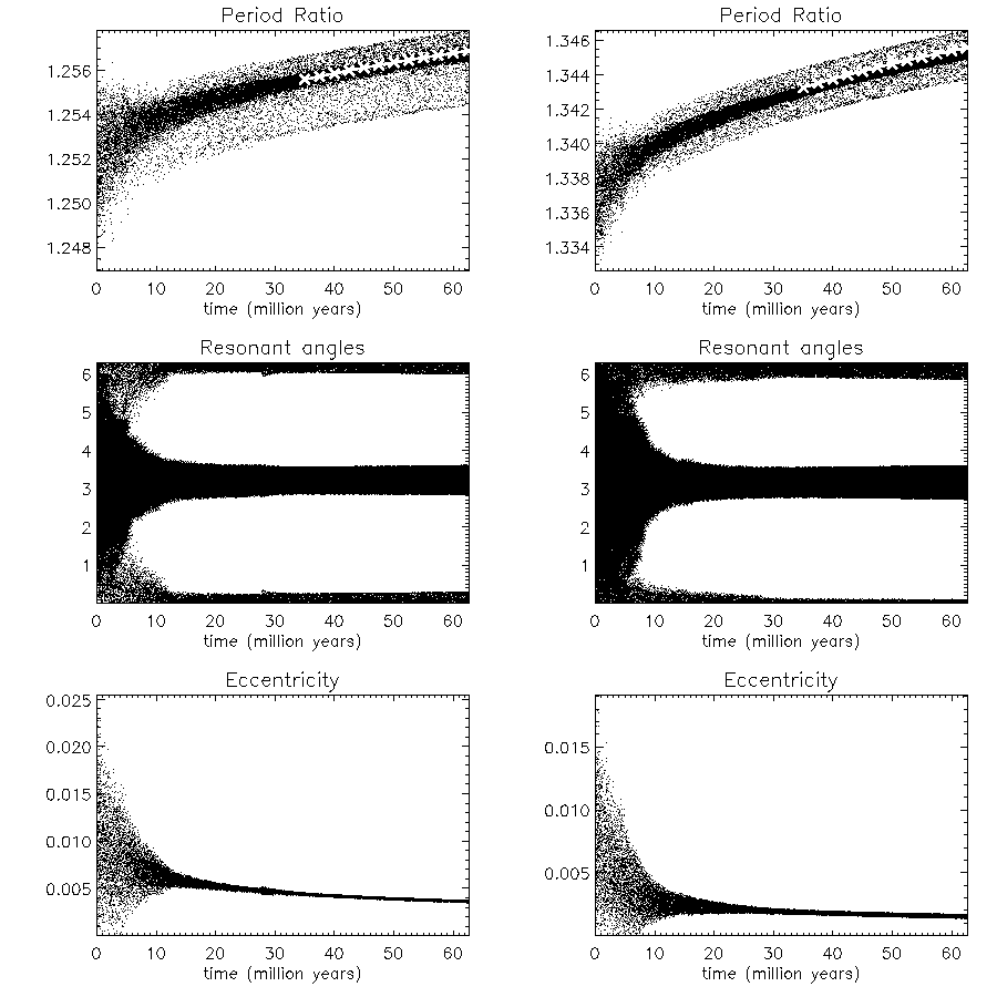
Figure 1: Results for $Q^{\prime}~{}=~{}2.5({\overline{\rho}}/2.4)^{-5/3}.$ The upper left panel show the evolution of the period ratio of the middle to innermost planet and the upper right panel shows the evolution of the period ratio of the outermost to middle planet. The curves marked with crosses are obtained from the analytic theory. Equation (51) was used as described in the text. The central left panel shows the evolution of the angles $\Phi_{1}$ and $\Phi_{2}$ which ultimately librate about $0$ and $\pi$ respectively. The central right panel shows the evolution of the angles $\Phi_{3}$ and $\Phi_{4}$ which ultimately librate about $0$ and $\pi$ respectively. The lower left and right panels show the evolution of the eccentricities on the middle and outermost planet respectively.

As values for the masses are not available, in order to estimate plausible values, unless specified otherwise, we use the fiducial mass-radius relation (see Lissauer et al. 2011)

$$m/M_{\oplus}\propto(R_{p}/R_{\oplus})^{2.06}.$$ (70)

We use equation (4) to calculate the circularization time. In order to implement this we need to specify the tidal parameter $Q^{\prime}.$ We note that according to (4), $t_{e,i}^{s}\propto Q^{\prime}{\overline{\rho}}^{5/3},$ where ${\overline{\rho}_{i}}^{5/3}$ is the mean density of planet $i.$ Quoted standard deviations in the radii amount to about 3 $\%$ for the inner two planets and 6 $\%$ for the outermost planet. To within these limits, using the masses calculated from (70), we may take the mean density, ${\overline{\rho}_{i}}=2.4\hskip 2.84526pt{\rm{g\hskip 2.84526ptcm^{-3}}}\equiv{\overline{\rho}},$ for each of the planets. Then, if we choose $Q^{\prime}=C_{Q^{\prime}}({\overline{\rho}}/2.4)^{-5/3}$ for planet $i,$ with $C_{Q^{\prime}}$ being a constant we can scale our results to apply to hypothetical planets with the same masses but with lower mean densities and thus larger $Q^{\prime}.$ Recall that $C_{Q^{\prime}}\equiv Q^{\prime}$ for the masses and radii given in table 1.

The simulations were by means of $N$–body calculations using the method described in eg. Papaloizou & Terquem (2001). From considerations of numerical tractability we are unable to consider very large values of $Q^{\prime}.$ In practice we took either $C_{Q^{\prime}}=2.5$ or $C_{Q^{\prime}}=7.5$ for each planet. However, in one case considered below, tidal dissipation was only applied to the innermost planet. Our general finding is that tidal dissipation causes the system to evolve into a state where a strict generalized Laplace resonance condition holds with all resonant angles maintained in a state of libration. The period ratios then increase with time with the system steadily separating from strict commensurability. This type evolution is very similar to that obtained for two planet systems under similar circumstances (eg. Papaloizou 2011).

4.1 Numerical Results

Planet	Radius	Mass	Mean density	Period	Period ratio
–	$R_{p}/R_{\oplus}$	$m/M_{\oplus}$	${\overline{\rho}}$	$P$	$(P_{i}/P_{i-1})$
1(b)	2.28	5.46	2.54 ${\rm{g\hskip 2.84526ptcm^{-3}}}$	7.1316185	–
2(c)	2.47	6.44	2.36 ${\rm{g\hskip 2.84526ptcm^{-3}}}$	8.9193459	1.2507
3(d)	2.55	6.88	2.29 ${\rm{g\hskip 2.84526ptcm^{-3}}}$	11.9016171	1.3344

Table 1: The radii, estimated masses, estimated mean densities and orbital periods in days for the three planets in the Kepler 60 system are given in the second to fifth columns respectively. The sixth column contains the period ratio with the next innermost planet where applicable.

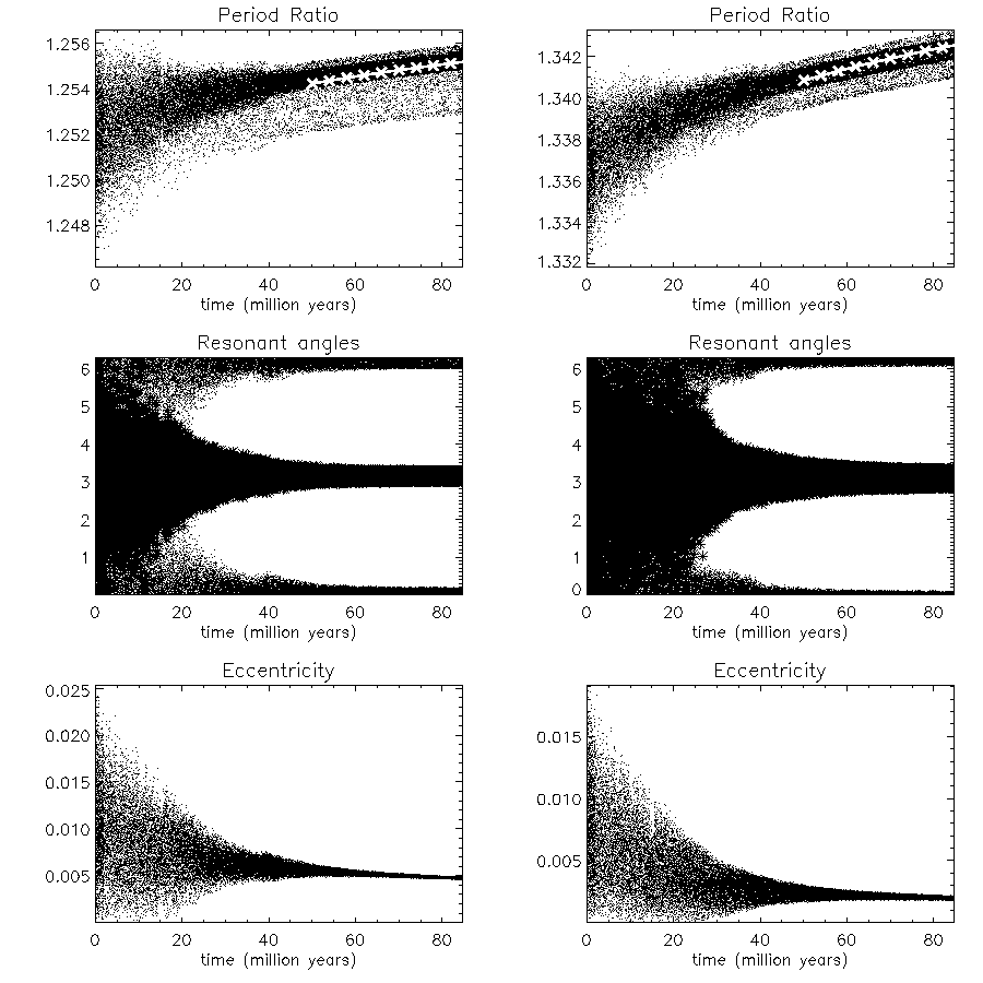
Figure 2: As for Fig. 1 but for $Q^{\prime}=7.5({\overline{\rho}}/2.4)^{-5/3}.$

The results obtained for a simulation with $Q^{\prime}~{}=~{}2.5({\overline{\rho}}/2.4)^{-5/3}$ are shown in in Fig. 1. The angles $\Phi_{1}$ and $\Phi_{2}$ initially circulate with the action of dissipation through tides ultimately causing them to librate with diminishing amplitude about $0$ and $\pi$ respectively. This evolution is well underway after a few million years. If the simulation was performed without tidal dissipation, variations in all quantities would remain at the same level with no tendency towards libration of the resonant angles. The angles $\Phi_{3}$ and $\Phi_{4}$ behave similarly to $\Phi_{1}$ and $\Phi_{2},$ ultimately librating about $0$ and $\pi$ respectively. This is all in accordance with the analytic model of section 3.5. The lower left and right panels of Fig. 1 show the evolution of the eccentricities on the middle and outermost planet respectively. As the librational state is attained, the eccentricities approach slowly decreasing values with superposed small oscillations. The period ratios of the middle to innermost planet and the middle to outermost planet then secularly increase as expected from the analytic model of section 3.5 for which the generalized three body Laplace relation is assumed to hold exactly. We have plotted expressions for the period ratios as a function of time obtained from equation (51) with $1/{\cal T}=1.81\times 10^{-13}$  yr${}^{-1},$ being the value calculated from the analytic model, and the integration constant $t_{0}=3.5\times 10^{6}$ yr. We recall that in this case $q=4,$ and the period ratios can be found from $|\Delta_{21}|$ by using $16/5(P_{2}/P_{1}-5/4)\sim|\Delta_{21}|/n_{1}$ and then the generalised three body Laplace relation to obtain the quantity $P_{3}/P_{2}-4/3.$ The curves marked with crosses represent these expressions which track the numerical data quite well. It is not clear exactly how the temporal fluctuations in the period ratios should be averaged when considering such fits. However, we remark that the lightly shaded regions in the period ratio plots are found to be associated with high frequency perturbations that are not represented in the analytic model. On the other hand, the darkly shaded regions are associated with longer period librations. Thus the fits should apply to the darkly shaded regions. We remark that the above analytically determined curves for $P_{2}/P_{1}$ and $P_{3}/P_{2},$ as well as others discussed below, obtained from equation (51), were calculated for positive values of $t_{0}$ that are comparable to the time for the resonant angles to begin circulating and which may be regarded as a characteristic time for transient behaviour. However, adopting $t_{0}=0$ produces curves that appear only slightly shifted from those presented.

We also performed a simulation with the same parameters except that tidal circularization applied only to the innermost planet. The evolution is similar to that described for the previous case but with the librational state taking longer to attain. We have evaluated expressions for the period ratios as a function of time obtained from equation (51), for $C_{Q^{\prime}}=2.5.$ but with tidal effects acting only on the inner planet. For this case we found that the numerical results were reasonably well represented when $1/{\cal T}=8.99\times 10^{-14}$ yr ^-1 as calculated from the analytic model, together with $t_{0}=3.5\times 10^{6}$ yr. From this we see that the secular evolution of the librating state occurs at a rate that is a factor of two slower when tides are applied only to the innermost planet.

4.1.1 Dependence on $Q^{\prime}$

In order to study the dependence of the evolution on $Q^{\prime},$ we show results for $Q^{\prime}=7.5({\overline{\rho}}/2.4)^{-5/3},$ with tidal effects applied to all the planets in Fig. 2. In this case the evolution towards the librational state is as for the case with $Q^{\prime}=2.5({\overline{\rho}}/2.4)^{-5/3}$ but three times slower as expected. This is apparent from the analytic curves obtained from equation (51). Thus we found $1/{\cal T}=6.04\times 10^{-14}~{}$yr^-1 and adopted $t_{0}=1.05\times 10^{7}$ yr for this case. In a similar manner, we have also confirmed the applicability of equation (51) for a run with $Q^{\prime}=0.75({\overline{\rho}}/2.4)^{-5/3},$ so that the range of $Q^{\prime}$ considered spans one order of magnitude.

4.1.2 Dependence on planet mass

We have explored the dependence of the evolution on planet mass by rerunning the case for which $Q^{\prime}=7.5({\overline{\rho}}/2.4)^{-5/3}$ with all of the planet masses increased by a factor of two while retaining a constant mean density. The results were found to be qualitatively similar but the evolutionary time scale is shorter. We see from equation (4) that the circularization time for each planet scales as $m^{-2/3}_{i}$ and so will be reduced by a factor of $2^{2/3}.$ Equation (LABEL:Delevfin) then implies that ${\cal T}$ scales as $m^{-8/3}_{i}$ and so should reduced by a factor $2^{8/3}.$ This is accurately confirmed by our curves determined from (51) that track the numerical data. These had $1/{\cal T}=3.83\times 10^{-13}$ yr^-1 and $t_{0}=5.5\times 10^{6}$ yr. We remark that if we had increased the planet masses by a factor of two while keeping their radii and $Q^{\prime}$ constant, equations (4) and (LABEL:Delevfin) would imply that ${\cal T}$ scales as $m^{-1}_{i}$ leading to a relatively weaker reduction in the evolution time. We also attempted simulations with the planet masses increased by a factor of four. However, these were found to lead to disruption of the system through instability within a time $<10^{6}$ yr.

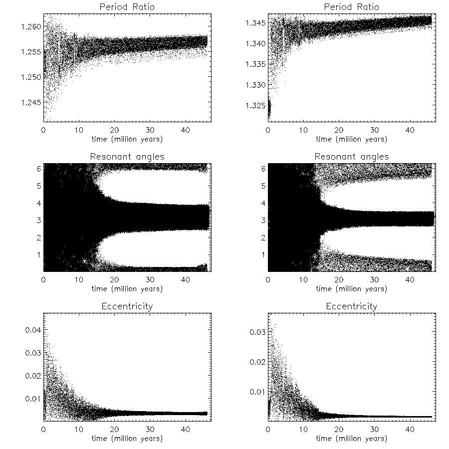
Figure 3: As in Fig. 1 but with different initial conditions described in the text.

4.1.3 A small variation of the initial period ratios

In this paper we have focused on initial conditions near to those appropriate to the Kepler 60 system. We remark that Marti et al. (2013) find that the Laplace resonance in the non dissipative GJ876 system is defined by a tiny island of regular motion surrounded by unstable highly chaotic orbits ( see also Gerlach & Haghighipour 2012). We comment that we found that some runs starting with slightly different initial conditions led to the same type of evolution as described above but took significantly longer to arrive at the librating state. We give results for the case with $C_{Q^{\prime}}=2.5,$ but with different initial conditions to those used previously, in Fig. 3. These were such that the semi-major axis of the outermost planet was decreased by a factor of $1.0050,$ while the semi-major axis of the central planet was decreased by a factor of $1.0007.$ With these changes the initial value of the period ratio $P_{2}/P_{1}$ changes from $1.2507$ to $1.2493$ and the initial value of the period ratio $P_{3}/P_{2}$ changes from $1.3344$ to $1.3259.$ Accordingly these are both below the values required for strict commensurability. This simulation ultimately attains the same libration state, with secular increasing period ratios, as the case with the original initial conditions. However, the initial period of time during which the resonant angles circulate and there are relatively large eccentricity oscillations is seen to last about twice as long at around $\sim 1.5\times 10^{7}$ yr in this case.

5 Discussion and conclusion

In this paper we have constructed a simple analytic model that describes the evolution of a three planet system in a three body resonance under the influence of tidal circularization. This is based on adopting a time averaged system for which contributions from a maximum of four resonant angles, associated with the first order resonances between the inner pair and outer pair of planets, are retained.

When all four angles undergo small amplitude libration the generalized three body Laplace relation is maintained while the period ratios increasingly depart from strict commensurability. But when only three of the resonance angles undergo small amplitude libration, the generalized three body Laplace relation was found to be replaced by a different relationship between the period ratios which depends on details such as the planet mass ratios and their orbital circularization time ratios.

Features of the analytic model such as the scaling of the evolution time scale with the planet mass scale, its dependence on tidal dissipation, and the form of the evolution of the period ratios away from commensurabilty were reproduced by our numerical simulations which were carried out for a three planet system with masses in the super-earth regime that were focussed on the Kepler 60 system for which the inner pair exhibit a 5:4 resonance and the outer pair exhibit a 4:3 resonance. However, we remark that much of the discussion should be generic.

We now briefly discuss how our results can be use to provide constraints on the amount of tidal dissipation that has occurred in such interacting systems. This discussion again adopts working parameters appropriate to the Kepler 60 system, though its form should again be generic. We remark that although Steffen et al. (2013) confirmed the Kepler 60 system by observing anti-correlated transit timing variations, low signal to noise parabolic, rather than periodic, variations are seen. Accordingly masses are not determined and whether resonant angles are in a librating state is unclear.

However, at the present time the inner and outer pair of planets are very close to 5:4 and 4:3 resonances respectively, with fractional deviations $\sim 10^{-3}.$ Such resonant chains are readily produced through convergent migration of protoplanets driven by interaction with the gas disk. Accordingly it is commonly assumed they were produced in this way while the gas disk was present (eg. Cresswell & Nelson 2006; Terquem & Papaloizou 2007; Thommes et al. 2008; Libert & Tsiganis 2011; Beaugé & Nesvorny 2012, Cossou et al. 2013) rather than through in situ formation, which tends to avoid resonances (Hansen & Murray; 2013). However, as noted by the former authors such resonant chains may be broken after the gas disperses by dynamical interactions and/or collisions with remaining planetesimals. Thus at a later time, but still shortly after formation, the system may differ to some extent from a putative initial resonant liberating state formed through convergent migration.

Although the above scenario forms a plausible basis for the origin of planetary systems that are very close to comprising a resonant chain, in principle the system could have started from a state that underwent tidal evolution of the type described here, with low $Q^{\prime},$ in such a way that the exact resonant state has been passed through only recently. However, noting that the evolution is most rapid in the resonant state this would seem to be unlikely. Accordingly, for the purposes of discussion, we shall assume that the system was formed close to the resonant state and consider how it would subsequently evolve as a result of tidal interactions with the central star.

We begin by estimating the time required for the system to attain a generalized three body Laplace resonance with all four resonance angles liberating with small amplitude. For simplicity in the discussion below, we assume that same $Q^{\prime}$ applies to all of the planets, noting extension to consider more general cases should be straightforward.

As expected, the evolution time scales in our simulations have been found to scale with the tidal dissipation parameter $Q^{\prime}.$ From the results presented in Figs. 1 and 2, the time required to attain a state in which the four resonant angles attain a state of small amplitude libration can be estimated to be $\sim 6.7\times 10^{6}C_{Q^{\prime}}$ yr. Here we assume, as indicated by these results that this time is in general proportional to $C_{Q^{\prime}}.$ Recall that $C_{Q^{\prime}}\equiv Q^{\prime}$ for ${\overline{\rho}_{i}}=2.4\hskip 2.84526pt{\rm{g\hskip 2.84526ptcm^{-3}}}$ as assumed here.

Although they do not provide an estimate of the age of the system, the stellar parameters given by Batalha et al. (2013) indicate that the star of mass $1.09M_{\odot},$ radius $1.5R_{\odot},$ and luminosity $2.5L_{\odot}$ is evolved. Accordingly, we shall adopt an age of $5\times 10^{9}$ yr in order to make illustrative estimates. Then failure to attain the librating state implies that $Q^{\prime}>\sim 750.$ This applies if $Q^{\prime}$ does not vary with time and the same for all planets (but see below). Should tides only operate on the innermost planet, the estimated bound on $Q^{\prime}$ should be reduced by a factor of two.

We now consider the expected evolution assuming that the system was formed in the four angle librating state. Then we note that if the system were actually in a three body resonance with small amplitude librations, the observed small deviations from exact commensurability would indicate a larger value of $Q^{\prime}$ than is given by the above bound. To show this, we consider the evolutionary time scale, $t_{ev},$ defined as the characteristic time required for $\Delta_{21}$ to undergo a relative change of order unity. Using (50), we find

$$t_{ev}=\left|\frac{\Delta_{21}}{d\Delta_{21}/dt}\right|=3\left(\frac{\Delta_{21}}{n_{1}}\right)^{3}{\cal T}=\frac{12288}{125}\left(\frac{P_{2}}{P_{1}}-\frac{5}{4}\right)^{3}{\cal T}$$ (71)

Using equations (LABEL:Delevfin) ond (50) while noting the scaling that ${\cal T}\propto C_{Q^{\prime}},$ we find that ${\cal T}=2.21\times 10^{12}C_{Q^{\prime}}$ yr. Thus

$$t_{ev}=2.17\times 10^{14}\left(\frac{P_{2}}{P_{1}}-\frac{5}{4}\right)^{3}C_{Q^{\prime}}\hskip 2.84526pt{\rm yr}.$$ (72)

Adopting the masses and period ratios in table 1 we then obtain

$$t_{ev}=7.44\times 10^{4}C_{Q^{\prime}}\hskip 2.84526pt{\rm yr}.$$ (73)

We recall that For the mean density ${\overline{\rho}}=2.4\hskip 2.84526pt{\rm{g\hskip 2.84526ptcm^{-3}}}$ adopted, $C_{Q^{\prime}}\equiv Q^{\prime}.$ In addition for fixed $Q^{\prime},$ planetary radii and planet mass ratios, $t_{ev}$ is inversely proportional to the planetary mass scale. Equation (73) implies that the system could not have begun in a three body resonance with four librating resonance angles and have its present period ratios if $C_{Q^{\prime}}<\sim 6.7\times 10^{4},$ this bound scaling with the mass scale. On the other hand if $C_{Q^{\prime}}>\sim 10^{3}$ the librating state would not have been attained through circularization.

Up to now we have assumed that $Q^{\prime}$ is constant. If $Q^{\prime}$ varies with time, as evolution rates are $\propto(Q^{\prime})^{-1},$ provided changes are slow enough for the system to respond adiabatically, the above estimates should relate to $\langle(Q^{\prime})^{-1}\rangle^{-1},$ where the angle brackets indicate a time average. This is effectively a statement that the amount of tidal dissipation has to have been limited. Thus although periods of strong episodic tidal heating of the type considered by Ojakangas & Stevenson (1986) may have occured, their integrated effect is constrained. We emphasise that the above estimates are provisional and that it should be possible to extend and refine the above discussion as more information about systems of this kind becomes available.

References

- (1) Barnes R., Jackson B., Raymond S. N., West A. A., Greenberg R., 2009, ApJ, 695, 1006
- (2) Batalha, N. M., Rowe, J. F., Bryson, S. T., et al. , 2013, ApJS, 204, 24
- (3) Batygin, K., Morbidelli, A., 2012, AJ, 145, 1
- (4) Beaugé, C., Nesvorny, D., 2012, ApJ, 751, 119
- (5) Brouwer D., Clemence G. M., 1961, Methods of celestial mechanics, New York: Academic Press
- (6) Correia, A. C. M., Couetdic, J., Laskar, J., Bonfils, X., Mayor, M., Bertaux, J.-L., Bouchy, F., Delfosse, X., Forveille, T., Lovis, C., Pepe, F., Perrier, C., Queloz, D., Udry, S., 2010, A& A, 511, id.A21
- (7) Cossou, C., Raymond, S. N., Pierens, A., 2013, A&A, 553, L2
- (8) Cresswell, P., Nelson, R.P., 2006, A&A, 450, 833.
- (9) Gerlach & Haghighipour , 2012, Cel. Mech. and Dynam. Astron., 113, 35
- (10) Goldreich P., Soter S., 1966, Icarus, 5, 375
- (11) Hansen, B.M. S., Murray, N., 2013, ApJ, 775, 53
- (12) Ivanov P. B., Papaloizou J. C. B., 2007, MNRAS, 376, 682
- (13) Kley, W., Nelson, R.P., 2012, ARA&A, 50, 211
- (14) Libert, A. S., Tsiganis, K., 2011, Cel. Mech. and Dynam. Astron., 111,201
- (15) Lissauer, J. J., Ragozine,D., Fabrycky, D. C., et al. 2011, ApJS, 197, 8
- (16) Lithwick, Y., Wu, Y., 2012, ApJ, 756, L11
- (17) Marti, J. G., Giuppone, C. A., Beauge, C., 2013, MNRAS, in press
- (18) Mayor M., Udry S., Lovis C., et al. 2009, A&A, 493, 639
- (19) Migaszewski, C., Sĺonina, M., Goździewski, K., 2012, MNRAS, 427, 770
- (20) Murray C. D., Dermott S. F., 1999, Solar System Dynamics (CUP), p. 254–255
- (21) Ojakangas, G. W., Stevenson, D. J., 1986, Icarus , 66, 341
- (22) Paardekooper S.–J, Mellema G., 2006, A&A, 459, L17
- (23) Papaloizou J.C.B., 2003, Cel. Mech. and Dynam. Astron., 87, 53
- (24) Papaloizou, J. C. B., 2011, Cel. Mech. and Dynam. Astron., 111, 83
- (25) Papaloizou J.C.B., Szuszkiewicz E., 2005, MNRAS, 363, 153
- (26) Papaloizou J.C.B., Terquem C., 2001, MNRAS, 325, 221
- (27) Papaloizou J.C.B., Terquem C., 2006, Rep. Prog. Phys., 69, 119
- (28) Papaloizou J.C.B., Terquem C., 2010, MNRAS, 405, 573
- (29) Raymond S. N., Barnes R., Mandell A. M., 2008, MNRAS, 384, 663
- (30) Sinclair A. T., 1975, MNRAS, 171, 59
- (31) Steffen, J. H., Fabrycky, D. C., Agol, E. , et al., 2013, MNRAS, 428, 1077
- (32) Terquem C., Papaloizou J. C. B., 2007, ApJ, 654, 1110
- (33) Thommes, E. W., Bryden, G., Wu, Y., Rasio, F. A., 2008, ApJ, 675, 1538
- (34) Ward W. R., 1997, Icarus, 126, 261