Estimation of Stable Distribution Parameters from a Dependent Sample

Abstract

Existing methods for the estimation of stable distribution parameters, such as those based on sample quantiles, sample characteristic functions or maximum likelihood generally assume an independent sample. Little attention has been paid to estimation from a dependent sample. In this paper, a method for the estimation of stable distribution parameters from a dependent sample is proposed based on the sample quantiles. The estimates are shown to be asymptotically normal. The asymptotic variance is calculated for stable moving average processes. Simulations from stable moving average (sma) processes are used to demonstrate these estimators.

1 Introduction

A number of methods have been proposed for the estimation of the parameters of a stable distribution have been proposed. A method based on sample quantiles was proposed by Fama and Roll (1971) which was simple to implement, but was only applicable to symmetric stable distributions with $\alpha\geq 1$ and contained a slight bias. This method was extended by McCulloch (1986) to cover asymmetric stable distributions and which is asymptotically unbiased. Other methods have been proposed based on the sample characteristic function, (Press (1972), Paulson et al. (1975) and Kogon and Williams (1998)). Maximum likelihood estimation methods have been proposed by Brorsen and Yang (1990) and Nolan (2001). For a discussion on the use of indirect inference for the estimation of stable distributions, see Garcia et al. (2011).

The sample quantile method of McCulloch (1986) assumes an independent sample. The primary goal of this paper is to investigate the extension of this method to cover dependent samples. For that purpose we use results on quantile estimation from dependent samples which show under certain conditions, these estimates are consistent and asymptotically normal (e.g. Sen (1968) and Dominicy et al. (2013)). We conclude with some simulations.

Throughout this paper we use the sma(q) process as an example of a dependent stable process. An sma(q) process $\{X_{t}\}$ is defined as follows

$$X_{t}=\sum_{j=0}^{q}\theta_{j}\varepsilon_{t-j}$$ (1)

where $\theta_{0}=1$ and $\{\varepsilon_{t}\}$ is an independent identically distributed (iid) sequence of stable random variables such that

$$\varepsilon_{t}\sim S_{\alpha}^{0}\left(\beta_{0},\gamma_{0},\delta_{0}\right)$$ (2)

using the $S^{0}$ parameterisation of stable random variables in Nolan (1998). Using the properties of the $S^{0}$ parameterisation given in Lemma 1, Nolan (1998) it can be shown that $X_{t}$ also has a stable distribution,

$$X_{t}\sim S_{\alpha}^{0}\left(\beta,\gamma,\delta\right).$$ (3)

Formulae for the stable distribution parameters of $X_{t}$ in terms of the sma(q) process parameters can be found in Barker (2014).

2 Quantile Estimation from a Dependent Sample

For any real-valued random variable $X$ on a probability space $\left(\Omega,\mathcal{F},P\right),$ there is an associated distribution function $F:\mathbb{R}\rightarrow\left[0,1\right]$ defined by

$$F\left(x\right)\equiv P\left(X\leq x\right).$$ (4)

The $p$th quantile, $\xi_{p}$, of $F$ is defined by

$$\xi_{p}\equiv\inf\left\{x:F\left(x\right)\leq p\right\}.$$ (5)

The density function, $f:\mathbb{R}\rightarrow\mathbb{R}_{+}$, of $F$ is defined by

$$F\left(x\right)\equiv\int_{-\infty}^{x}f\left(s\right)ds.$$ (6)

Let $\left\{x_{j}\right\}_{j=1}^{n}$ be a sample drawn from random variables with the distribution function $F$. From this sample we define the empirical distribution function and empirical quantile estimators by

$$\widehat{F}_{n}\left(x\right)=\dfrac{1}{n}\sum_{j=1}^{n}I_{\left(-\infty,x\right]}\left(x_{j}\right),$$ (7)

and

$$\widehat{\xi}_{p}=\inf\left\{x:\widehat{F}_{n}\left(x\right)\geq p\right\}.$$ (8)

There is an extensive literature about the statistical properties of the empirical estimators (e.g. Cramer (1946) and Serfling (1980)).

The following theorems assume that $\left\{x_{j}\right\}_{j=1}^{n}$ is an iid sample. The first theorem shows that the empirical quantile estimator has strong consistency wherever the underlying distribution function is not flat.

Theorem 1

(Strong Consistency of $\widehat{\xi}_{p}$ - Serfling (1980), Theorem 2.3.1). Let $0<p<1.$ If $\xi_{p}$ is the unique solution $x$ of $F\left(x_{-}\right)\leq p\leq F\left(x\right),$ then $\widehat{\xi}_{p}$ is a strongly consistent estimator of $\xi_{p}.$

The next theorem shows that the empirical quantile estimator is asymptotically normal under some conditions on the underlying distribution function (See also Cramer (1946))

Theorem 2

(Asymptotic Normality of Empirical Quantile Estimator - Serfling (1980), Corollary 2.3.3B). For $0<p<1,$ if $F$ possesses a density $f$ in a neighbourhood of $\xi_{p}$ and if $f$ is positive and continuous at $\xi_{p},$ then

$$\widehat{\xi}_{p}\text{ is }AN\left(\xi_{p},\dfrac{p\left(1-p\right)}{f^{2}\left(\xi_{p}\right)n}\right).$$ (9)

Theorem 2 can be extended to cover the estimation of multiple quantiles from a single sample.

Theorem 3

(Asymptotic Covariances of Empirical Quantile Estimators - Serfling (1980), Theorem 2.3.3B). Let $0<p_{1}<\cdots<p_{k}<1.$ Suppose that $F$ has a density $f$ in a neighbourhoods of $\xi_{p_{1}},\ldots,\xi_{p_{k}}$ and that $f$ is positive and continuous at $\xi_{p_{1}},\ldots,\xi_{p_{k}}.$ Let $\widehat{\xi}=\left(\widehat{\xi}_{p_{1}},\ldots,\widehat{\xi}_{p_{k}}\right)^{\prime}$ denote the empirical quantiles estimates of $\xi=\left(\xi_{p_{1}},\ldots,\xi_{p_{k}}\right)^{\prime},$ then

$$\sqrt{n}\left(\widehat{\xi}-\xi\right)\overset{d}{\longrightarrow}N\left(0,\Sigma\right).$$ (10)

The element in the $ith$ row and $jth$ column of $\Sigma$ is given by

$$\sigma_{ij}=\left\{\begin{array}[]{cc}\dfrac{p_{i}\left(1-p_{j}\right)}{f\left(\xi_{p_{i}}\right)f\left(\xi_{p_{j}}\right)}&\text{ for }i\leq j\\ \dfrac{p_{j}\left(1-p_{i}\right)}{f\left(\xi_{p_{i}}\right)f\left(\xi_{p_{j}}\right)}&\text{ for }i>j\end{array}\right.$$ (11)

The asymptotic distributions listed in Theorems 2 and 3 only apply if the sample $\left\{x_{j}\right\}_{j=1}^{n}$ is iid. The asymptotic distribution of the empirical quantile estimator, where the sample is taken from a possibly non-stationary m-dependent process was derived by Sen (1968). Further work in this area has been done by, amongst others: Dutta and Sen (1971) on autoregressive processes, Sen (1972) on $\phi$ - mixing processes, Oberhofer and Haupt (2005) on non-stationary processes and Dominicy et al. (2013) on S-mixing processes. In this paper, we use the results of Dominicy et al. (2013) for S-mixing processes.

Definition 1

(S-mixing Process - Berkes et al. (2009)). A process $\left\{\mathbf{X}_{t}\right\}$ is called S-mixing if it satisfies the following conditions

1. For any $t\in\mathbb{Z}$ and $m\in\mathbb{N},$ one can find a random variable $\mathbf{X}_{tm}$ such that

   $$P\left(\left|\mathbf{X}_{t}-\mathbf{X}_{tm}\right|\geq\gamma_{m}\right)\leq\delta_{m}$$ (12)

   for some numerical sequences $\gamma_{m}\rightarrow 0,\delta_{m}\rightarrow 0.$

2. For any disjoint intervals $I_{1},\ldots,I_{r}$ of integers and any positive integers $m_{1},\ldots,m_{r},$ the vectors $\left\{\mathbf{X}_{tm_{1}},t\in I_{1}\right\},\ldots,\left\{\mathbf{X}_{tm_{r}},t\in I_{r}\right\}$ are independent provided the separation between $I_{k}$ and $I_{l}$ is greater than $m_{k}+m_{l}.$

An sma process is an S-mixing process (Berkes et al. (2009)) and also a $\phi$ - mixing process (e.g. Davidson (1994)). Other examples of S-mixing processes can be found in Berkes et al. (2009) and Dominicy et al. (2013).

Let

$$\mathbf{X}_{t}=g\left(e_{t},e_{t-1},\ldots\right),\quad t\in\mathbb{Z}$$ (13)

be a $k$ - dimensional process where $\left\{e_{t}\right\}$ is an iid sequence of elements from the measurable space $\Omega$ and $g:\Omega^{\infty}\rightarrow\mathbb{R}^{k}$ is a measurable function. The following theorem from Dominicy et al. (2013) provides the asymptotic distribution for the empirical quantile estimators from a multivariate S-mixing process. Note that Theorem 6.5 in Sen (1972) proves a similar result for $\phi$ - mixing processes

Theorem 4

(Dominicy et al. (2013), Theorem 1). Let $\left\{\mathbf{X}_{t}\right\}$ be a stationary process satisfying $\left(\ref{eq:qe:10}\right)$ and let $\mathbf{\xi}=\left(\xi_{1},\ldots,\xi_{k}\right)^{\prime}$ denote the quantiles of $\left\{\mathbf{X}_{t}\right\}$ at $\mathbf{p}=\left(p_{1},\ldots,p_{k}\right)^{\prime}.$ Suppose that

A1 For each $i$ in $1,\ldots,k$ the marginal distribution function $F_{i}\left(x\right)$ has a density $f_{i}\left(x\right)$ that is positive and continuous in the neighbourhood of $\xi_{i}$ and $f_{i}\left(x\right)$ is uniformly bounded by some constant $B.$

A2 The process $\left\{\mathbf{X}_{t}\right\}$ is S-mixing with coefficients $\gamma_{m}=\delta_{m}=O\left(m^{-A}\right)$ where $A>4.$

Then

$$\sqrt{n}\left(\widehat{\mathbf{\xi}}-\mathbf{\xi}\right)\overset{d}{\longrightarrow}N\left(0,\Sigma\right)$$ (14)

where

$$\Sigma = V^{-1}QV^{-1},$$ (15)

$$V = diag\left(f_{1}\left(\xi_{1}\right),\ldots,f_{k}\left(\xi_{k}\right)\right),$$ (16)

$$Q = \sum_{h\in\mathbb{Z}}E\left[Q_{0}Q_{h}^{\prime}\right],$$ (17)

$$Q_{j} = \left(I\left\{X_{j;1}\leq\xi_{1}\right\}-p_{1},\ldots,I\left\{X_{j;k}\leq\xi_{k}\right\}-p_{k}\right).$$ (18)

The element is the $ith$ row and $jth$ column of the matrix $\Sigma$ is given by

$$\sigma_{ij}=\dfrac{\sum_{h\in\mathbb{Z}}\left(P\left(\left\{X_{t;i}\leq\xi_{i}\right\}\cap\left\{X_{t+h;j}\leq\xi_{j}\right\}\right)-p_{i}p_{j}\right)}{f_{i}\left(\xi_{i}\right)f_{j}\left(\xi_{j}\right)}.$$ (19)

Remark 1

Note that all stable distributions satisfy Assumption A1 and that all arma processes satisfy Assumption A2

Remark 2

Whilst Theorem 4 applies to the estimation of a single quantile from each component of a vector process, it can be adapted for the joint estimation of multiple quantiles from a scalar process $\left\{X_{t}\right\}$ through application to the vector process

$$\left\{\mathbf{X}_{t}\right\}=\left(X_{t},\ldots,X_{t}\right)^{\prime}$$ (20)

In order to calculate the asymptotic variance, $\Sigma$, of the empirical quantile estimates from a scalar S-mixing process $\left\{X_{t}\right\}$, it is necessary to calculate the joint probabilities

$$G_{h}\left(\xi_{i},\xi_{j}\right)=P\left(\left\{X_{t}\leq\xi_{i}\right\}\cap\left\{X_{t+h}\leq\xi_{j}\right\}\right)$$ (21)

for each $h\in\mathbb{Z}$. For $h=0,$ $\left(\ref{eq:qe:18}\right)$ can be simplified to give

$$G_{0}\left(\xi_{i},\xi_{j}\right)=\min\left(p_{i},p_{j}\right)$$ (22)

For $h\neq 0,$ the evaluation of $\left(\ref{eq:qe:18}\right)$ whilst theoretically possible for some S-mixing processes is computationally very difficult for many. For an sma(q) process, the independence of $X_{t}$ and $X_{t+h}$ for all $\left|h\right|>q$ means that $\left(\ref{eq:qe:16}\right)$ can be simplified to

$$\sigma_{ij}=\dfrac{\sum_{h=-q}^{q}\left(G_{h}\left(\xi_{i},\xi_{j}\right)-p_{i}p_{j}\right)}{f\left(\xi_{i}\right)f\left(\xi_{j}\right)}.$$ (23)

For an iid process we get

$$G_{h}\left(\xi_{i},\xi_{j}\right)=0,\quad\text{for }h\neq 0.$$ (24)

Thus for iid processes, Theorem 3 produces the same asymptotic covariance matrix as Theorem 4.

Suppose $\{X_{t}\}$ is an sma(1) process and let $f$ and $F$ denote the density and distribution functions respectively of the associated innovation sequence $\left\{\varepsilon_{t}\right\}$. Then

$$G_{1}\left(\xi_{i},\xi_{j}\right) = P\left(\left\{\varepsilon_{t}+\theta_{1}\varepsilon_{t-1}\leq\xi_{i}\right\}\cap\left\{\varepsilon_{t+1}+\theta_{1}\varepsilon_{t}\leq\xi_{j}\right\}\right)$$ (25)

$$= P\left(\left\{\varepsilon_{t-1}\leq\dfrac{\xi_{i}-\varepsilon_{t}}{\theta_{1}}\right\}\cap\left\{\varepsilon_{t+1}\leq\xi_{j}-\theta_{1}\varepsilon_{t}\right\}\right)$$

$$= \int_{-\infty}^{\infty}F\left(\dfrac{\xi_{i}-u}{\theta_{1}}\right)F\left(\xi_{j}-\theta_{1}u\right)f\left(u\right)du,$$

which can be evaluated numerically. Note that

$$G_{1}\left(\xi_{i},\xi_{j}\right)=G_{-1}\left(\xi_{j},\xi_{i}\right)$$ (26)

For higher order sma(q) processes, the evaluation of $G_{h}\left(\xi_{i},\xi_{j}\right)$ becomes computationally difficult, involving a $q-1+h$ dimensional integral. However the estimation of $G_{h}\left(\xi_{i},\xi_{j}\right)$ is straightforward. Let $\left\{x_{t}\right\}_{t=1}^{n}$ be a sample of size $n$ from the sma(q) process $\left\{X_{t}\right\}.$ We define the estimator $\widehat{G}_{h}\left(\xi_{i},\xi_{j}\right)$ as

$$\widehat{G}_{h}\left(\xi_{i},\xi_{j}\right)=\left(n-h\right)^{-1}\sum_{t=1}I\left\{x_{t}\leq\xi_{i}\right\}\cdot I\left\{x_{t+h}\leq\xi_{j}\right\},\quad\text{for }\left|h\right|>1$$ (27)

and it is clear that $\widehat{G}_{h}\left(\xi_{i},\xi_{j}\right)$ is a consistent estimator of $G_{h}\left(\xi_{i},\xi_{j}\right).$ For the purposes of this paper we do not consider the asymptotic properties of $\widehat{G}_{h}\left(\xi_{i},\xi_{j}\right).$

3 Estimation of Stable Distribution Parameters

The following method for the estimation of stable distribution parameters was proposed in McCulloch (1986). Let $\xi_{p}$ denote the $pth$ quantile of the stable distribution $S_{\alpha}^{0}\left(\beta,\gamma,\delta\right)$ and define the following statistics

$$v_{\alpha} = \dfrac{\xi_{0.95}-\xi_{0.05}}{\xi_{0.75}-\xi_{0.25}},$$ (28)

$$v_{\beta} = \dfrac{\xi_{0.95}+\xi_{0.05}-2\xi_{0.50}}{\xi_{0.95}-\xi_{0.05}}.$$ (29)

These statistics do not depend on $\gamma,\delta$ and so we can consider them as functions solely of $\alpha,\beta,$

$$v_{\alpha} = \phi_{1}\left(\alpha,\beta\right),$$ (30)

$$v_{\beta} = \phi_{2}\left(\alpha,\beta\right).$$ (31)

It can be seen that $\phi_{1}\left(\alpha,\beta\right)$ is a strictly decreasing function of $\alpha$ for each $\beta$ and that $\phi_{2}\left(\alpha,\beta\right)$ is a strictly decreasing function of $\beta$ for each $\alpha.$ The relationships $\left(\ref{eq:est:2a}\right)$ and $\left(\ref{eq:est:2b}\right)$ can be inverted to give

$$\alpha = \psi_{1}\left(v_{\alpha},v_{\beta}\right),$$ (32)

$$\beta = \psi_{2}\left(v_{\alpha},v_{\beta}\right).$$ (33)

Let $\widehat{\xi}_{p}$ denote a consistent estimator for $\xi_{p}$. Substituting the estimators $\widehat{\xi}_{p}$ into $\left(\ref{eq:est:1a}\right)$ and $\left(\ref{eq:est:1b}\right)$ gives consistent estimators for $v_{\alpha},v_{\beta},$

$$\widehat{v}_{\alpha} = \dfrac{\widehat{\xi}_{0.95}-\widehat{\xi}_{0.05}}{\widehat{\xi}_{0.75}-\widehat{\xi}_{0.25}},$$ (34)

$$\widehat{v}_{\beta} = \dfrac{\widehat{\xi}_{0.95}+\widehat{\xi}_{0.05}-2\widehat{\xi}_{0.50}}{\widehat{\xi}_{0.95}-\widehat{\xi}_{0.05}}.$$ (35)

Consistent estimators for the parameters $\alpha,\beta$ can then be calculated using

$$\widehat{\alpha} = \psi_{1}\left(\widehat{v}_{\alpha},\widehat{v}_{\beta}\right),$$ (36)

$$\widehat{\beta} = \psi_{2}\left(\widehat{v}_{\alpha},\widehat{v}_{\beta}\right).$$ (37)

Under the $S^{0}$ parameterisation of the stable distribution, the parameters $\gamma$ and $\delta$ act respectively as scale and location parameters of the distribution. We formalise this property in the following lemma.

Lemma 1

Let

$$X\sim S_{\alpha}^{0}\left(\beta,\gamma,\delta\right)$$ (38)

and

$$X^{*}\sim S_{\alpha}^{0}\left(\beta,1,0\right)$$ (39)

be stable random variables. Let $\xi_{p}$ and $\xi_{p}^{*}$ denote respectively the $p$th quantile of $X$ and $X^{*}$. Then for any $0<p_{1},p_{2}<1$ where $p_{1}\neq p_{2}$ we have

$$\gamma=\dfrac{\xi_{p_{2}}-\xi_{p_{1}}}{\xi_{p_{2}}^{*}-\xi_{p_{1}}^{*}}$$ (40)

and

$$\delta=\xi_{p_{1}}-\gamma\xi_{p_{1}}^{*}$$ (41)

Proof. From Lemma 1 (Nolan (1998)), we have

$$\gamma X^{*}+\delta\sim X.$$ (42)

It follows that for any $0<p<1$

$$\xi_{p}^{*}=\dfrac{\xi_{p}-\delta}{\gamma},$$ (43)

from which (40) and (41) follow immediately.   

We can use the results of Lemma 41 to define the estimators of $\gamma$ and $\delta$ by

$$\widehat{\gamma}=\dfrac{\widehat{\xi}_{0.75}-\widehat{\xi}_{0.25}}{\widehat{\xi}_{0.75}^{*}-\widehat{\xi}_{0.25}^{*}}$$ (44)

and

$$\widehat{\delta}=\widehat{\xi}_{0.50}-\widehat{\gamma}\widehat{\xi}_{0.50}^{*}.$$ (45)

where $\widehat{\xi}_{p}^{*}$ is the $pth$ quantile of the distribution $S_{\widehat{\alpha}}^{0}(\widehat{\beta},1,0)$. The estimators in (44) and (45) are similar to those defined in McCulloch (1986). The differences are due to McCulloch’s choice of parameterisation for the stable distribution, which includes discontinuities at $\alpha=1$.

From Lemma 41, it can be seen that other choices of quantile levels are available to define $\widehat{\gamma}$ and $\widehat{\delta}$. For computational efficiency, it is preferable to choose from the same quantile levels used to define $\widehat{\alpha}$ and $\widehat{\beta}$. Indeed, other choices of quantile levels are also available to define $\widehat{\alpha}$ and $\widehat{\beta}$ and it is possible that a different choice of quantile levels would produce better estimators.

Let

$$\widehat{\xi}_{M}=\left(\widehat{\xi}_{0.05},\widehat{\xi}_{0.25},\widehat{\xi}_{0.50},\widehat{\xi}_{0.75},\widehat{\xi}_{0.95}\right)^{\prime}$$ (46)

denote the empirical quantile estimates of

$$\xi_{M}=\left(\xi_{0.05},\xi_{0.25},\xi_{0.50},\xi_{0.75},\xi_{0.95}\right)^{\prime}$$ (47)

from an S-mixing process $\{X_{t}\}$. Let $\Sigma_{M}$ denote the asymptotic covariance matrix of $\widehat{\xi}_{M}$ obtained from Theorem 4. We define the matrix of partial derivatives $D$ by

$$D=\left(\begin{array}[]{ccccc}\dfrac{\partial\widehat{\alpha}}{\partial\widehat{\xi}_{0.05}}&\dfrac{\partial\widehat{\alpha}}{\partial\widehat{\xi}_{0.25}}&\dfrac{\partial\widehat{\alpha}}{\partial\widehat{\xi}_{0.50}}&\dfrac{\partial\widehat{\alpha}}{\partial\widehat{\xi}_{0.75}}&\dfrac{\partial\widehat{\alpha}}{\partial\widehat{\xi}_{0.95}}\\ \dfrac{\partial\widehat{\beta}}{\partial\widehat{\xi}_{0.05}}&\dfrac{\partial\widehat{\beta}}{\partial\widehat{\xi}_{0.25}}&\dfrac{\partial\widehat{\beta}}{\partial\widehat{\xi}_{0.50}}&\dfrac{\partial\widehat{\beta}}{\partial\widehat{\xi}_{0.75}}&\dfrac{\partial\widehat{\beta}}{\partial\widehat{\xi}_{0.95}}\\ \dfrac{\partial\widehat{\gamma}}{\partial\widehat{\xi}_{0.05}}&\dfrac{\partial\widehat{\gamma}}{\partial\widehat{\xi}_{0.25}}&\dfrac{\partial\widehat{\gamma}}{\partial\widehat{\xi}_{0.50}}&\dfrac{\partial\widehat{\gamma}}{\partial\widehat{\xi}_{0.75}}&\dfrac{\partial\widehat{\gamma}}{\partial\widehat{\xi}_{0.95}}\\ \dfrac{\partial\widehat{\delta}}{\partial\widehat{\xi}_{0.05}}&\dfrac{\partial\widehat{\delta}}{\partial\widehat{\xi}_{0.25}}&\dfrac{\partial\widehat{\delta}}{\partial\widehat{\xi}_{0.50}}&\dfrac{\partial\widehat{\delta}}{\partial\widehat{\xi}_{0.75}}&\dfrac{\partial\widehat{\delta}}{\partial\widehat{\xi}_{0.95}}\end{array}\right)^{\prime},$$ (48)

then following the same approach taken by in McCulloch (1986) using the Multivariate Delta Theorem (see Serfling (1980)), we obtain

$$\sqrt{n}\left(\left(\begin{array}[]{c}\widehat{\alpha}\\ \widehat{\beta}\\ \widehat{\gamma}\\ \widehat{\delta}\end{array}\right)-\left(\begin{array}[]{c}\alpha\\ \beta\\ \gamma\\ \delta\end{array}\right)\right)\overset{d}{\longrightarrow}N\left(0,D^{\prime}\Sigma_{M}D\right).$$ (49)

A general analytic formula is not available for the calculation of the partial derivatives in $\left(\ref{eq:est:15}\right)$. It is suggested in McCulloch (1986) that the partial derivatives can be estimated “by means of small perturbations of the population quantiles”, but no specific recommendations regarding the size of these perturbations are given. To limit the scope of our investigation into this matter, we restrict ourselves to perturbations given by

$$\Delta\xi=\dfrac{\widehat{\xi}_{0.75}-\widehat{\xi}_{0.25}}{C}$$ (50)

for some $C>0$ and assume that the same perturbation is applied to each quantile estimator. Let $\widehat{\alpha}_{p}^{+}$ be the estimate of $\alpha$ derived from the set of quantiles where $\widehat{\xi}_{p}$ is replaced by $\widehat{\xi}_{p}+\Delta\xi$ and $\widehat{\alpha}_{p}^{-}$ be the estimate of $\alpha$ derived from the set of quantile estimates where $\widehat{\xi}_{p}$ is replaced by $\widehat{\xi}_{p}-\Delta\xi.$ Similarly, we define $\widehat{\beta}_{p}^{+},~{}\widehat{\beta}_{p}^{-},$ etc. Our estimate for $\dfrac{\partial\widehat{\alpha}}{\partial\widehat{\xi}_{p}}$ is defined to be

$$\widehat{\dfrac{\partial\widehat{\alpha}}{\partial\widehat{\xi}_{p}}}=\dfrac{\widehat{\alpha}_{p}^{+}-\widehat{\alpha}_{p}^{-}}{2\Delta\xi}$$ (51)

with similar definitions for $\widehat{\dfrac{\partial\widehat{\beta}}{\partial\widehat{\xi}_{p}}},\widehat{\dfrac{\partial\widehat{\gamma}}{\partial\widehat{\xi}_{p}}}$ and $\widehat{\dfrac{\partial\widehat{\delta}}{\partial\widehat{\xi}_{p}}}.$

Estimates for each of the partial derivative estimators were calculated for various stable distributions. Examples of these calculations are presented in Figure 1 for values of $C$ between 50 and 1000. The optimal choice for $C$ is not obvious, given we do not have any true values for the partial derivatives. However, in general the value of the partial derivative estimates does not change greatly for $C$ between 50 and 1000. A slightly lower value of $C\$and hence slightly larger perturbation can help to smooth the partial derivatives and avoid occasional numerical abberations. Throughout this paper we use $C=400$, to calculate the partial derivative estimates. In Figure 1, the estimates calculated using $C=400$ are those indicated by fourth ${}^{\prime}\ast^{\prime}$ from the left.

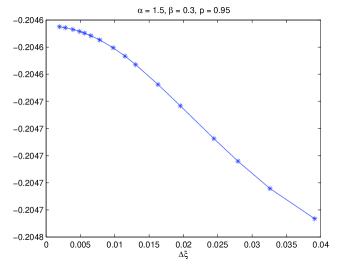
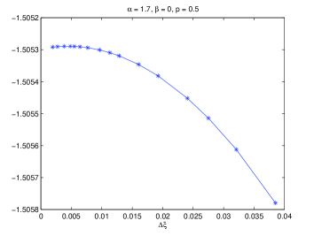
(a)	(b)

Figure 1: Estimates for (a) $\dfrac{\partial\widehat{\alpha}}{\partial\widehat{\xi}_{0.95}}$ where $\alpha=1.5$ and $\beta=0.3$ and (b) $\dfrac{\partial\widehat{\beta}}{\partial\widehat{\xi}_{0.50}}$ where $\alpha=1.7$ and $\beta=0.0$.

With some minor modifications by the author, the matlab package stbl_code was used throughout this paper to generate sequences of stable random variable, calculate values of the stable density, distribution and quantile functions. To implement stable distribution parameter estimation, a lookup table for $\psi_{1}$ and $\psi_{2}$ with $184$ values of $v_{\alpha}$ and $86$ values of $v_{\beta}$ was generated. Interpolation is used to calculate the values of $\psi_{1}$ and $\psi_{2}$ for those values of $v_{\alpha}$ and $v_{\beta}$ which do not exactly match the lookup table values. Spline interpolation is used in preference to linear interpolation, except for $\alpha$ close to $2,$ where spline interpolation occasionally performs poorly. All partial derivatives in Figure 1 were calculated using spline interpolation. If linear interpolation was used to calculate the derivatives in Figure 1, then the resulting plots would show discontinuities in the first derivative at points where the values of $v_{\alpha}$ and $v_{\beta}$ move between cells in the lookup tables.

4 Simulation

In this section we present the results of some simulations which demonstrate the use of the methods described in this paper for the estimation of the stable distribution parameters of a sma(1) process. For selected set of values $\alpha$, $\beta$, and $\theta_{1}$ a simulation is run where 2,000 realisations of the process, each of length $n=720$, are generated . The parameters $\gamma_{0}=2$ and $\delta_{0}=1$ are fixed for all simulations. Estimates for the parameters $\alpha$, $\beta$, $\gamma$ and $\delta$ are calculated for each realisation. The mean and variance of these estimates across all realisations of a particular simulation are then compared with the true parameter values and the asymptotic variance of the estimators. The results for $\alpha$, $\beta$, $\gamma$ and $\delta$ are reported in Tables 1, 2, 3 and 4 respectively.

		$\theta_{1}=0.0$		$\theta_{1}=0.2$		$\theta_{1}=0.4$
$\alpha$	$\beta$	(i)	(ii)	(i)	(ii)	(i)	(ii)
$1.2$	$0.0$	$\begin{array}[]{c}\text{{\small 1.195}}\\ \text{{\small(0.061)}}\end{array}$	$\begin{array}[]{c}\text{{\small 2.682}}\\ \text{{\small[2.555]}}\end{array}$	$\begin{array}[]{c}\text{{\small 1.195}}\\ \text{{\small(0.063)}}\end{array}$	$\begin{array}[]{c}\text{{\small 2.891}}\\ \text{{\small[2.740]}}\end{array}$	$\begin{array}[]{c}\text{{\small 1.194}}\\ \text{{\small(0.068)}}\end{array}$	$\begin{array}[]{c}\text{{\small 3.322}}\\ \text{{\small[3.200]}}\end{array}$
$1.2$	$0.2$	$\begin{array}[]{c}\text{{\small 1.196}}\\ \text{{\small(0.062)}}\end{array}$	$\begin{array}[]{c}\text{{\small 2.746}}\\ \text{{\small[2.833]}}\end{array}$	$\begin{array}[]{c}\text{{\small 1.199}}\\ \text{{\small(0.067)}}\end{array}$	$\begin{array}[]{c}\text{{\small 3.224}}\\ \text{{\small[3.040]}}\end{array}$	$\begin{array}[]{c}\text{{\small 1.198}}\\ \text{{\small(0.072)}}\end{array}$	$\begin{array}[]{c}\text{{\small 3.702}}\\ \text{{\small[3.568]}}\end{array}$
$1.2$	$0.5$	$\begin{array}[]{c}\text{{\small 1.202}}\\ \text{{\small(0.076)}}\end{array}$	$\begin{array}[]{c}\text{{\small 4.134}}\\ \text{{\small[3.975]}}\end{array}$	$\begin{array}[]{c}\text{{\small 1.201}}\\ \text{{\small(0.076)}}\end{array}$	$\begin{array}[]{c}\text{{\small 4.204}}\\ \text{{\small[4.257]}}\end{array}$	$\begin{array}[]{c}\text{{\small 1.200}}\\ \text{{\small(0.084)}}\end{array}$	$\begin{array}[]{c}\text{{\small 5.074}}\\ \text{{\small[5.058]}}\end{array}$
$1.5$	$0.0$	$\begin{array}[]{c}\text{{\small 1.503}}\\ \text{{\small(0.076)}}\end{array}$	$\begin{array}[]{c}\text{{\small 4.105}}\\ \text{{\small[3.852]}}\end{array}$	$\begin{array}[]{c}\text{{\small 1.504}}\\ \text{{\small(0.079)}}\end{array}$	$\begin{array}[]{c}\text{{\small 4.472}}\\ \text{{\small[3.984]}}\end{array}$	$\begin{array}[]{c}\text{{\small 1.502}}\\ \text{{\small(0.080)}}\end{array}$	$\begin{array}[]{c}\text{{\small 4.604}}\\ \text{{\small[4.348]}}\end{array}$
$1.5$	$0.2$	$\begin{array}[]{c}\text{{\small 1.504}}\\ \text{{\small(0.078)}}\end{array}$	$\begin{array}[]{c}\text{{\small 4.346}}\\ \text{{\small[4.076]}}\end{array}$	$\begin{array}[]{c}\text{{\small 1.506}}\\ \text{{\small(0.081)}}\end{array}$	$\begin{array}[]{c}\text{{\small 4.693}}\\ \text{{\small[4.217]}}\end{array}$	$\begin{array}[]{c}\text{{\small 1.505}}\\ \text{{\small(0.087)}}\end{array}$	$\begin{array}[]{c}\text{{\small 5.466}}\\ \text{{\small[4.611]}}\end{array}$
$1.5$	$0.5$	$\begin{array}[]{c}\text{{\small 1.505}}\\ \text{{\small(0.087)}}\end{array}$	$\begin{array}[]{c}\text{{\small 5.384}}\\ \text{{\small[5.207]}}\end{array}$	$\begin{array}[]{c}\text{{\small 1.506}}\\ \text{{\small(0.091)}}\end{array}$	$\begin{array}[]{c}\text{{\small 5.907}}\\ \text{{\small[5.384]}}\end{array}$	$\begin{array}[]{c}\text{{\small 1.506}}\\ \text{{\small(0.094)}}\end{array}$	$\begin{array}[]{c}\text{{\small 6.375}}\\ \text{{\small[5.919]}}\end{array}$
$1.8$	$0.0$	$\begin{array}[]{c}\text{{\small 1.808}}\\ \text{{\small(0.108)}}\end{array}$	$\begin{array}[]{c}\text{{\small 8.389}}\\ \text{{\small[9.471]}}\end{array}$	$\begin{array}[]{c}\text{{\small 1.809}}\\ \text{{\small(0.107)}}\end{array}$	$\begin{array}[]{c}\text{{\small 8.160}}\\ \text{{\small[9.544]}}\end{array}$	$\begin{array}[]{c}\text{{\small 1.809}}\\ \text{{\small(0.109)}}\end{array}$	$\begin{array}[]{c}\text{{\small 8.495}}\\ \text{{\small[9.783]}}\end{array}$
$1.8$	$0.2$	$\begin{array}[]{c}\text{{\small 1.810}}\\ \text{{\small(0.109)}}\end{array}$	$\begin{array}[]{c}\text{{\small 8.515}}\\ \text{{\small[9.536]}}\end{array}$	$\begin{array}[]{c}\text{{\small 1.808}}\\ \text{{\small(0.110)}}\end{array}$	$\begin{array}[]{c}\text{{\small 8.678}}\\ \text{{\small[9.611]}}\end{array}$	$\begin{array}[]{c}\text{{\small 1.806}}\\ \text{{\small(0.109)}}\end{array}$	$\begin{array}[]{c}\text{{\small 8.614}}\\ \text{{\small[9.853]}}\end{array}$
$1.8$	$0.5$	$\begin{array}[]{c}\text{{\small 1.809}}\\ \text{{\small(0.106)}}\end{array}$	$\begin{array}[]{c}\text{{\small 8.083}}\\ \text{{\small[9.902]}}\end{array}$	$\begin{array}[]{c}\text{{\small 1.808}}\\ \text{{\small(0.108)}}\end{array}$	$\begin{array}[]{c}\text{{\small 8.353}}\\ \text{{\small[9.981]}}\end{array}$	$\begin{array}[]{c}\text{{\small 1.809}}\\ \text{{\small(0.110)}}\end{array}$	$\begin{array}[]{c}\text{{\small 8.669}}\\ \text{{\small[10.24]}}\end{array}$

Table 1: Simulation results of the estimation of $\alpha$ from selected sma(1) processes. Reported in this table for each process are (i) the mean and standard deviation, in ( ), of $\widehat{\alpha}$ across all realisations and (ii) the variance of $\widehat{\alpha}$ across all realisations multiplied by the sample size $n$ and the true asymptotic variance, in [ ].

In each case the mean value of the estimator across all realisations is within one standard deviation of the true parameter value and is generally much closer than that. The normalised variance (i.e. the variance multiplied by the sample size) across all realisations is reasonably close to the asymptotic variance.

The normalised variance of $\widehat{\alpha}$ where $\alpha=1.8$ appears to be slightly less than the asymptotic variance. This is due to the truncation of all $\widehat{\alpha}$ estimates into the range $\left(0,2\right].$ A similar effect is seen with $\widehat{\beta}$ estimates where $\alpha=1.8$ and $\beta_{0}=0.5$. Estimates of $\widehat{\beta}$ where $\alpha=1.8$ are the least precise. This is to be expected as the asymptotic variance of $\widehat{\beta}$ increases to $\infty$ as $\alpha$ increases to 2.

For each of the selected sma(1) processes and for each of the estimators $\widehat{\alpha}$, $\widehat{\beta}$, $\widehat{\gamma}$ and $\widehat{\delta}$ the asymptotic variance of the estimator is higher for $\theta_{1}=0.2$ than for $\theta_{1}=0.0$ and higher still for $\theta_{1}=0.4.$ The effect of increases in $\theta_{1}$ on the asymptotic variance of the estimators $\widehat{\alpha}$, $\widehat{\beta}$, $\widehat{\gamma}$ and $\widehat{\delta}$ appears to decrease as $\alpha$ increases and is more significant for $\widehat{\gamma}$ and $\widehat{\delta}$ than for $\widehat{\alpha}$ and $\widehat{\beta}$. From additional simulation results not included in this paper, we observe that the asymptotic variance of $\widehat{\gamma}$ appears symmetric in $\theta_{1}$ about zero, however that does not appear to be the case for $\widehat{\alpha}$, $\widehat{\beta}$ and $\widehat{\delta}$ where more complicated relationships exist between the asymptotic variances and the parameter values.

		$\theta_{1}=0.0$		$\theta_{1}=0.2$		$\theta_{1}=0.4$
$\alpha$	$\beta$	(i)	(ii)	(i)	(ii)	(i)	(ii)
$1.2$	$0.0$	$\begin{array}[]{c}\text{{\small 0.000}}\\ \text{{\small(0.105)}}\end{array}$	$\begin{array}[]{c}\text{{\small 7.961}}\\ \text{{\small[8.684]}}\end{array}$	$\begin{array}[]{c}\text{{\small 0.002}}\\ \text{{\small(0.121)}}\end{array}$	$\begin{array}[]{c}\text{{\small 10.46}}\\ \text{{\small[10.91]}}\end{array}$	$\begin{array}[]{c}\text{{\small 0.001}}\\ \text{{\small(0.131)}}\end{array}$	$\begin{array}[]{c}\text{{\small 12.30}}\\ \text{{\small[12.94]}}\end{array}$
$1.2$	$0.2$	$\begin{array}[]{c}\text{{\small 0.193}}\\ \text{{\small(0.101)}}\end{array}$	$\begin{array}[]{c}\text{{\small 7.408}}\\ \text{{\small[7.677]}}\end{array}$	$\begin{array}[]{c}\text{{\small 0.196}}\\ \text{{\small(0.113)}}\end{array}$	$\begin{array}[]{c}\text{{\small 9.230}}\\ \text{{\small[9.657]}}\end{array}$	$\begin{array}[]{c}\text{{\small 0.194}}\\ \text{{\small(0.124)}}\end{array}$	$\begin{array}[]{c}\text{{\small 11.03}}\\ \text{{\small[11.44]}}\end{array}$
$1.2$	$0.5$	$\begin{array}[]{c}\text{{\small 0.498}}\\ \text{{\small(0.082)}}\end{array}$	$\begin{array}[]{c}\text{{\small 4.866}}\\ \text{{\small[4.223]}}\end{array}$	$\begin{array}[]{c}\text{{\small 0.495}}\\ \text{{\small(0.089)}}\end{array}$	$\begin{array}[]{c}\text{{\small 5.751}}\\ \text{{\small[5.199]}}\end{array}$	$\begin{array}[]{c}\text{{\small 0.494}}\\ \text{{\small(0.098)}}\end{array}$	$\begin{array}[]{c}\text{{\small 6.852}}\\ \text{{\small[6.046]}}\end{array}$
$1.5$	$0.0$	$\begin{array}[]{c}\text{{\small-0.001}}\\ \text{{\small(0.127)}}\end{array}$	$\begin{array}[]{c}\text{{\small 11.60}}\\ \text{{\small[11.67]}}\end{array}$	$\begin{array}[]{c}\text{{\small 0.001}}\\ \text{{\small(0.140)}}\end{array}$	$\begin{array}[]{c}\text{{\small 14.10}}\\ \text{{\small[13.27]}}\end{array}$	$\begin{array}[]{c}\text{{\small 0.000}}\\ \text{{\small(0.151)}}\end{array}$	$\begin{array}[]{c}\text{{\small 16.44}}\\ \text{{\small[15.52]}}\end{array}$
$1.5$	$0.2$	$\begin{array}[]{c}\text{{\small 0.202}}\\ \text{{\small(0.140)}}\end{array}$	$\begin{array}[]{c}\text{{\small 14.06}}\\ \text{{\small[11.16]}}\end{array}$	$\begin{array}[]{c}\text{{\small 0.204}}\\ \text{{\small(0.139)}}\end{array}$	$\begin{array}[]{c}\text{{\small 13.88}}\\ \text{{\small[12.60]}}\end{array}$	$\begin{array}[]{c}\text{{\small 0.203}}\\ \text{{\small(0.151)}}\end{array}$	$\begin{array}[]{c}\text{{\small 16.33}}\\ \text{{\small[14.63]}}\end{array}$
$1.5$	$0.5$	$\begin{array}[]{c}\text{{\small 0.525}}\\ \text{{\small(0.147)}}\end{array}$	$\begin{array}[]{c}\text{{\small 15.44}}\\ \text{{\small[11.44]}}\end{array}$	$\begin{array}[]{c}\text{{\small 0.522}}\\ \text{{\small(0.152)}}\end{array}$	$\begin{array}[]{c}\text{{\small 16.70}}\\ \text{{\small[12.24]}}\end{array}$	$\begin{array}[]{c}\text{{\small 0.520}}\\ \text{{\small(0.156)}}\end{array}$	$\begin{array}[]{c}\text{{\small 17.57}}\\ \text{{\small[13.45]}}\end{array}$
$1.8$	$0.0$	$\begin{array}[]{c}-\text{{\small 0.008}}\\ \text{{\small(0.367)}}\end{array}$	$\begin{array}[]{c}\text{{\small 97.20}}\\ \text{{\small[53.62]}}\end{array}$	$\begin{array}[]{c}\text{{\small 0.008}}\\ \text{{\small(0.369)}}\end{array}$	$\begin{array}[]{c}\text{{\small 97.76}}\\ \text{{\small[55.74]}}\end{array}$	$\begin{array}[]{c}\text{{\small 0.000}}\\ \text{{\small(0.375)}}\end{array}$	$\begin{array}[]{c}\text{{\small 101.5}}\\ \text{{\small[60.59]}}\end{array}$
$1.8$	$0.2$	$\begin{array}[]{c}\text{{\small 0.223}}\\ \text{{\small(0.367)}}\end{array}$	$\begin{array}[]{c}\text{{\small 97.40}}\\ \text{{\small[63.83]}}\end{array}$	$\begin{array}[]{c}\text{{\small 0.202}}\\ \text{{\small(0.381)}}\end{array}$	$\begin{array}[]{c}\text{{\small 104.4}}\\ \text{{\small[65.85]}}\end{array}$	$\begin{array}[]{c}\text{{\small 0.186}}\\ \text{{\small(0.380)}}\end{array}$	$\begin{array}[]{c}\text{{\small 104.1}}\\ \text{{\small[70.58]}}\end{array}$
$1.8$	$0.5$	$\begin{array}[]{c}\text{{\small 0.488}}\\ \text{{\small(0.334)}}\end{array}$	$\begin{array}[]{c}\text{{\small 80.51}}\\ \text{{\small[118.5]}}\end{array}$	$\begin{array}[]{c}\text{{\small 0.488}}\\ \text{{\small(0.347)}}\end{array}$	$\begin{array}[]{c}\text{{\small 86.49}}\\ \text{{\small[120.0]}}\end{array}$	$\begin{array}[]{c}\text{{\small 0.484}}\\ \text{{\small(0.353)}}\end{array}$	$\begin{array}[]{c}\text{{\small 89.85}}\\ \text{{\small[124.1]}}\end{array}$

Table 2: Simulation results of the estimation of $\beta$ from selected sma(1) processes. Reported in this table for each process are (i) the mean and standard deviation, in ( ), of $\widehat{\beta}$ across all realisations and (ii) the variance of $\widehat{\beta}$ across all realisations multiplied by the sample size $n$ and the true asymptotic variance, in [ ].

These simulations provide some confidence that the estimators discussed in this paper, are an unbiased method for the estimation of stable distribution parameters from a sma(1) process and that the asymptotic variance provides a good approximation for estimator variance at sample sizes equal to 720.

		$\theta_{1}=0.0$			$\theta_{1}=0.4$
$\alpha$	$\beta$	$\gamma$	(i)	(ii)	$\gamma$	(i)	(ii)
$1.2$	$0.0$	2.000	$\begin{array}[]{c}\text{{\small 1.991}}\\ \text{{\small(0.104)}}\end{array}$	$\begin{array}[]{c}\text{{\small 7.751}}\\ \text{{\small[7.983]}}\end{array}$	2.541	$\begin{array}[]{c}\text{{\small 2.523}}\\ \text{{\small(0.153)}}\end{array}$	$\begin{array}[]{c}\text{{\small 16.82}}\\ \text{{\small[16.32]}}\end{array}$
$1.2$	$0.2$	2.000	$\begin{array}[]{c}\text{{\small 1.992}}\\ \text{{\small(0.112)}}\end{array}$	$\begin{array}[]{c}\text{{\small 9.000}}\\ \text{{\small[8.648]}}\end{array}$	2.541	$\begin{array}[]{c}\text{{\small 2.535}}\\ \text{{\small(0.156)}}\end{array}$	$\begin{array}[]{c}\text{{\small 17.58}}\\ \text{{\small[17.52]}}\end{array}$
$1.2$	$0.5$	2.000	$\begin{array}[]{c}\text{{\small 2.001}}\\ \text{{\small(0.123)}}\end{array}$	$\begin{array}[]{c}\text{{\small 10.83}}\\ \text{{\small[10.80]}}\end{array}$	2.541	$\begin{array}[]{c}\text{{\small 2.543}}\\ \text{{\small(0.171)}}\end{array}$	$\begin{array}[]{c}\text{{\small 21.14}}\\ \text{{\small[21.15]}}\end{array}$
$1.5$	$0.0$	2.000	$\begin{array}[]{c}\text{{\small 2.000}}\\ \text{{\small(0.097)}}\end{array}$	$\begin{array}[]{c}\text{{\small 6.822}}\\ \text{{\small[6.553]}}\end{array}$	2.325	$\begin{array}[]{c}\text{{\small 2.322}}\\ \text{{\small(0.120)}}\end{array}$	$\begin{array}[]{c}\text{{\small 10.32}}\\ \text{{\small[10.45]}}\end{array}$
$1.5$	$0.2$	2.000	$\begin{array}[]{c}\text{{\small 1.997}}\\ \text{{\small(0.094)}}\end{array}$	$\begin{array}[]{c}\text{{\small 6.290}}\\ \text{{\small[6.633]}}\end{array}$	2.325	$\begin{array}[]{c}\text{{\small 2.318}}\\ \text{{\small(0.120)}}\end{array}$	$\begin{array}[]{c}\text{{\small 10.37}}\\ \text{{\small[10.54]}}\end{array}$
$1.5$	$0.5$	2.000	$\begin{array}[]{c}\text{{\small 2.000}}\\ \text{{\small(0.098)}}\end{array}$	$\begin{array}[]{c}\text{{\small 6.838}}\\ \text{{\small[6.877]}}\end{array}$	2.325	$\begin{array}[]{c}\text{{\small 2.321}}\\ \text{{\small(0.125)}}\end{array}$	$\begin{array}[]{c}\text{{\small 11.24}}\\ \text{{\small[10.77]}}\end{array}$
$1.8$	$0.0$	2.000	$\begin{array}[]{c}\text{{\small 2.000}}\\ \text{{\small(0.093)}}\end{array}$	$\begin{array}[]{c}\text{{\small 6.162}}\\ \text{{\small[6.272]}}\end{array}$	2.205	$\begin{array}[]{c}\text{{\small 2.204}}\\ \text{{\small(0.108)}}\end{array}$	$\begin{array}[]{c}\text{{\small 8.407}}\\ \text{{\small[8.482]}}\end{array}$
$1.8$	$0.2$	2.000	$\begin{array}[]{c}\text{{\small 2.000}}\\ \text{{\small(0.094)}}\end{array}$	$\begin{array}[]{c}\text{{\small 6.417}}\\ \text{{\small[6.267]}}\end{array}$	2.205	$\begin{array}[]{c}\text{{\small 2.200}}\\ \text{{\small(0.108)}}\end{array}$	$\begin{array}[]{c}\text{{\small 8.378}}\\ \text{{\small[8.473]}}\end{array}$
$1.8$	$0.5$	2.000	$\begin{array}[]{c}\text{{\small 2.003}}\\ \text{{\small(0.093)}}\end{array}$	$\begin{array}[]{c}\text{{\small 6.146}}\\ \text{{\small[6.227]}}\end{array}$	2.205	$\begin{array}[]{c}\text{{\small 2.210}}\\ \text{{\small(0.111)}}\end{array}$	$\begin{array}[]{c}\text{{\small 8.799}}\\ \text{{\small[8.408]}}\end{array}$

Table 3: Simulation results of the estimation of $\gamma$ from selected sma(1) processes. Reported in this table for each process are (i) the mean and standard deviation, in ( ), of $\widehat{\gamma}$ across all realisations and (ii) the variance of $\widehat{\gamma}$ across all realisations multiplied by the sample size $n$ and the true asymptotic variance, in [ ].

		$\theta_{1}=0.0$			$\theta_{1}=0.4$
$\alpha$	$\beta$	$\delta$	(i)	(ii)	$\delta$	(i)	(ii)
$1.2$	$0.0$	1.000	$\begin{array}[]{c}\text{{\small 0.998}}\\ \text{{\small(0.130)}}\end{array}$	$\begin{array}[]{c}\text{{\small 12.15}}\\ \text{{\small[13.05]}}\end{array}$	1.400	$\begin{array}[]{c}\text{{\small 1.398}}\\ \text{{\small(0.194)}}\end{array}$	$\begin{array}[]{c}\text{{\small 27.04}}\\ \text{{\small[28.32]}}\end{array}$
$1.2$	$0.2$	1.000	$\begin{array}[]{c}\text{{\small 1.003}}\\ \text{{\small(0.134)}}\end{array}$	$\begin{array}[]{c}\text{{\small 12.95}}\\ \text{{\small[13.19]}}\end{array}$	1.559	$\begin{array}[]{c}\text{{\small 1.558}}\\ \text{{\small(0.197)}}\end{array}$	$\begin{array}[]{c}\text{{\small 27.97}}\\ \text{{\small[28.62]}}\end{array}$
$1.2$	$0.5$	1.000	$\begin{array}[]{c}\text{{\small 1.001}}\\ \text{{\small(0.139)}}\end{array}$	$\begin{array}[]{c}\text{{\small 14.00}}\\ \text{{\small[14.11]}}\end{array}$	1.798	$\begin{array}[]{c}\text{{\small 1.812}}\\ \text{{\small(0.208)}}\end{array}$	$\begin{array}[]{c}\text{{\small 31.15}}\\ \text{{\small[30.41]}}\end{array}$
$1.5$	$0.0$	1.000	$\begin{array}[]{c}\text{{\small 1.001}}\\ \text{{\small(0.143)}}\end{array}$	$\begin{array}[]{c}\text{{\small 14.73}}\\ \text{{\small[15.49]}}\end{array}$	1.400	$\begin{array}[]{c}\text{{\small 1.397}}\\ \text{{\small(0.200)}}\end{array}$	$\begin{array}[]{c}\text{{\small 28.71}}\\ \text{{\small[27.46]}}\end{array}$
$1.5$	$0.2$	1.000	$\begin{array}[]{c}\text{{\small 1.005}}\\ \text{{\small(0.148)}}\end{array}$	$\begin{array}[]{c}\text{{\small 15.73}}\\ \text{{\small[15.61]}}\end{array}$	1.495	$\begin{array}[]{c}\text{{\small 1.500}}\\ \text{{\small(0.198)}}\end{array}$	$\begin{array}[]{c}\text{{\small 28.22}}\\ \text{{\small[27.68]}}\end{array}$
$1.5$	$0.5$	1.000	$\begin{array}[]{c}\text{{\small 0.993}}\\ \text{{\small(0.150)}}\end{array}$	$\begin{array}[]{c}\text{{\small 16.27}}\\ \text{{\small[16.58]}}\end{array}$	1.638	$\begin{array}[]{c}\text{{\small 1.633}}\\ \text{{\small(0.201)}}\end{array}$	$\begin{array}[]{c}\text{{\small 29.09}}\\ \text{{\small[29.24]}}\end{array}$
$1.8$	$0.0$	1.000	$\begin{array}[]{c}\text{{\small 0.997}}\\ \text{{\small(0.160)}}\end{array}$	$\begin{array}[]{c}\text{{\small 18.49}}\\ \text{{\small[19.50]}}\end{array}$	1.400	$\begin{array}[]{c}\text{{\small 1.395}}\\ \text{{\small(0.202)}}\end{array}$	$\begin{array}[]{c}\text{{\small 29.35}}\\ \text{{\small[30.46]}}\end{array}$
$1.8$	$0.2$	1.000	$\begin{array}[]{c}\text{{\small 1.010}}\\ \text{{\small(0.159)}}\end{array}$	$\begin{array}[]{c}\text{{\small 18.15}}\\ \text{{\small[19.61]}}\end{array}$	1.439	$\begin{array}[]{c}\text{{\small 1.454}}\\ \text{{\small(0.199)}}\end{array}$	$\begin{array}[]{c}\text{{\small 28.62}}\\ \text{{\small[30.59]}}\end{array}$
$1.8$	$0.5$	1.000	$\begin{array}[]{c}\text{{\small 1.018}}\\ \text{{\small(0.160)}}\end{array}$	$\begin{array}[]{c}\text{{\small 18.35}}\\ \text{{\small[20.10]}}\end{array}$	1.497	$\begin{array}[]{c}\text{{\small 1.512}}\\ \text{{\small(0.203)}}\end{array}$	$\begin{array}[]{c}\text{{\small 29.80}}\\ \text{{\small[31.24]}}\end{array}$

Table 4: Simulation results of the estimation of $\delta$ from selected sma(1) processes. Reported in this table for each process are (i) the mean and standard deviation, in ( ), of $\widehat{\delta}$ across all realisations and (ii) the variance of $\widehat{\delta}$ across all realisations multiplied by the sample size $n$ and the true asymptotic variance, in [ ].

References

• Barker (2014) Barker, A., 2014. On the log quantile difference of the temporal aggregation of a stable moving average process URL: http://arxiv.org/abs/1404.6875. preprint, Macquarie University.
• Berkes etΒ al. (2009) Berkes, I., HΓΆrmann, S., Schauer, J., 2009. Asymptotic results for the empirical process of stationary sequences. Stochastic Processes and their Applications 119, 1298–1324.
• Brorsen and Yang (1990) Brorsen, B., Yang, S., 1990. Maximum likelihood estimates of symmetric stable distribution parameters. Communications in Statistics - Simulation and Computation 19, 1459–1464.
• Cramer (1946) Cramer, H., 1946. Mathematical Methods of Statistics. Princeton University Press.
• Davidson (1994) Davidson, J., 1994. Stochastic Limit Theory: An Introduction for Econometricians. Oxford University Press.
• Dominicy etΒ al. (2013) Dominicy, Y., Hormann, S., Ogata, H., Veredas, D., 2013. On sample marginal quantiles for stationary processes. Statistics and Probability Letters 83, 28–36.
• Dutta and Sen (1971) Dutta, K., Sen, P., 1971. On the Bahadur representation of sample quantiles in some stationary multivariate autoregressive processes. Journal of Multivariate Analysis 1, 186–198.
• Fama and Roll (1971) Fama, E., Roll, R., 1971. Parameter estimates for symmetric stable distributions. Journal of the American Statistical Association 66, 331–338.
• Garcia etΒ al. (2011) Garcia, R., Renault, E., Veredas, D., 2011. Estimation of stable distributions by indirect inference. Journal of Econometrics 161, 325–337.
• Kogon and Williams (1998) Kogon, S., Williams, D., 1998. Characteristic function based estimation of stable distribution parameters, in: Adler, R., Feldman, R., Taqqu, M. (Eds.), A Practical Guide to Heavy Tails: Statistical Techniques and Applications. BirkhΓ€user.
• McCulloch (1986) McCulloch, J., 1986. Simple consistent estimators of stable distribution parameters. Communications in Statistics - Simulation and Computation 15, 1109–1136.
• Nolan (1998) Nolan, J., 1998. Parameterizations and modes of stable distributions. Statistics and Probability Letters 38, 187–195.
• Nolan (2001) Nolan, J., 2001. Maximum likelihood estimation of stable parameters, in: Barndorff-Nielsen, O., Mikosch, T., Resnick, I. (Eds.), Levy Processes: Theory and Application. BirkhΓ€user.
• Oberhofer and Haupt (2005) Oberhofer, W., Haupt, H., 2005. The asymptotic distribution of the unconditional quantile estimator under dependence. Statistics and Probability Letters 73, 243–250.
• Paulson etΒ al. (1975) Paulson, A., Holcomb, E., Leitch, R., 1975. The estimation of the parameters of the stable laws. Biometrika 62, 163–170.
• Press (1972) Press, S., 1972. Estimation in univariate and multivariate stable distributions. Journal of the Americal Statistical Association 67, 842–846.
• Sen (1968) Sen, P., 1968. Asymptotic normality of sample quantiles for m-dependent processes. The Annals of Mathematical Statistics 39, 1724–1730.
• Sen (1972) Sen, P., 1972. On the Bahadur representation of sample quantiles for sequences of $\phi$ - mixing random variables. Journal of Multivariate Analysis 2, 77–95.
• Serfling (1980) Serfling, R., 1980. Approximation Theorems of Mathematical Statistics. Wiley.