An efficient algorithm for T-estimation

Abstract

We introduce an efficient and exact algorithm, together with a faster but approximate version, which implements with a sub-quadratic complexity the hold-out derived from T-estimation. We study empirically the performance of this hold-out in the context of density estimation considering well-known competitors (hold-out derived from least-squares or Kullback-Leibler divergence, model selection procedures, etc.) and classical problems including histogram or bandwidth selection. Our algorithms are integrated in a companion R-package called Density.T.HoldOut available on the CRAN: http://cran.r-project.org/web/packages/Density.T.HoldOut/index.html.

Index terms— T-estimation; density estimation; hold-out; Density.T.HoldOut; R-package

1 Introduction

Suppose we have at hand a sample of independent and identically distributed (i.i.d.) random variables from some unknown density $s$ with respect to some dominating measure $\mu$ and that we want to estimate $s$ from the sample.

Many papers have been published about the solution of this estimation problem with as little prior information on $s$ as possible. A widely used strategy consists in starting from a family of preliminary estimators (for instance kernel or histogram estimators) with some varying smoothing parameter (the bandwidth or the partition) and selecting one candidate using the sample. Nevertheless, since the 30’s (Larson, 1931) it has been known that building estimators and evaluating their quality with the same data yields an overoptimistic result. Many solutions exist to overcome this problem. One natural procedure - called hold-out - consists in splitting the sample into two subsamples, building a family of estimators using the first subsample (which we shall call the training sample) and making the selection using the second subsample (which we shall call the validation sample).

Concerning the selection part, Birgé (2006, Section 9) proposed a procedure - called T-hold-out hereafter - based on robust tests between the preliminary estimators. The procedure can be derived from Birgé’s construction of T-estimators oriented to model selection. The definition of these estimators is introduced in the same paper but relies on old ideas arising from Le Cam (1973); Birgé (1983, 1984a, 1984b). Indeed, conditionally to the training sample, all the estimators are deterministic so that the models are reduced to points and the problem amounts to select one point from the validation sample.

The purpose of this paper is to provide an efficient algorithm that implements the T-hold-out, made available in our R-package called Density.T.HoldOut. Our motivations are twofold. First, when we started this research in the summer of 2012 there was no practical application of T-estimation and we were very surprised to observe that most authors - including Birgé himself - considered this procedure only as a theoretical tool, because of its supposed “too high computational complexity” as pointed out in Birgé (2006), Birgé (2007, p.45) and Baraud and Birgé (2009, p.241). Second, we thought it would be of interest to compare empirically T-estimation with classical resampling and penalization procedures since they are motivated by risk estimation, whereas T-estimators are based on robust tests and thus enjoy some robustness properties. For this purpose we considered several finite collections of preliminary estimators. These included histogram or kernel collections - leading to some well-known estimation problems: number of bin selection, partition selection, bandwidth selection, but also more complex collections mixing histograms and kernel estimators potentially completed with some parametric ones. The scripts, developed for this paper using our R-package, are available on the RunMyCode website (http://www.runmycode.org) to increase transparency and reproducibility.

Hold-out is not specific to the density framework. Indeed, in all cases where we have at hand two independent random samples $\textbf{X}_{t}$ and $\textbf{X}_{v}$, one can build a collection of estimators using the training sample $\textbf{X}_{t}$ and proceed to the selection with the validation sample $\textbf{X}_{v}$. In density estimation, hold-out has been investigated theoretically for projection estimators (Arlot and Lerasle, 2014, Section 8.1) and kernel density estimates (Devroye and Lugosi, 2001) among other examples. Searching for the best linear (or convex) combination of the preliminary estimators in the validation step leads to the linear (or convex) aggregation problem (see Rigollet and Tsybakov (2007)). Moreover, theoretical properties of the hold-out have also been studied in classification (Bartlett et al., 2002; Blanchard and Massart, 2006) and in regression -by Lugosi and Nobel (1999); Juditsky and Nemirovski (2000); Nemirovski (2000); Wegkamp (2003), among others.

1.1 Framework

Let us consider a sample $\textbf{X}=\left\{\left.X_{1},\ldots,X_{n}\right.\right\}$ of i.i.d. random variables $X_{i}$ with values in the measured space $(\mathcal{X},\mathcal{W},\mu)$. We suppose that the distribution of $X_{i}$ admits a density $s$ with respect to $\mu$ and aim to estimate $s$. We turn the set $\mathcal{S}$ of all probability densities with respect to $\mu$ into a metric space using the Hellinger distance $h(t,u)$ where

$$h^{2}(t,u)=\frac{1}{2}\int\left(\left.\sqrt{t(x)}-\sqrt{u(x)}\right.\right)^{2}d\mu(x)\enspace.$$

Although Birgé’s procedure relies on this distance, we shall also consider $L_{q}$-distances - derived from $L_{q}$-norms denoted $\|.\|_{q}$ - for $q=1,2$.

The quality of an approximation $t\in\mathcal{S}$ of the function $s$ is measured by $\ell(t,s)$, where $\ell$ is a loss function (typically some power of a distance). The risk of an estimator $\tilde{s}=\tilde{s}(\textbf{X})$ of the function $s$ is defined through this loss function by $R_{s}(\tilde{s},\ell):=\mathbb{E}_{s}[\ell(\tilde{s},s)]$, where $\mathbb{E}_{s}$ denotes the expectation when $s$ obtains. The Hellinger risk $R_{s}(\tilde{s},h^{2})$ comes from the loss $\ell=h^{2}$. The loss can also be defined as $\ell(t,s)=\mathbb{E}_{s}[\gamma(t,X)-\gamma(s,X)]$, where $\gamma:\mathcal{S}\times\mathcal{X}\mapsto[0,\infty)$ is a contrast function for which $s$ appears as a minimizer of $\mathbb{E}_{s}[\gamma(t,X)]$ when $t\in\mathcal{S}$ (Birgé and Massart, 1993, Definition 1). In this context, the $L_{2}$-loss (resp. the Kullback-Leibler loss) is defined via the contrast function $\gamma(t,x)=\|t\|_{2}^{2}-2t(x)$ (resp. $\gamma(t,x)=-\log(t(x))$) for any $t\in\mathcal{S}$, $x\in\mathcal{X}$.

1.2 About the Hold-Out

Formally, the hold-out (HO) is a two-steps estimation procedure which relies on a split of X into two non-empty complementary subsamples, $\textbf{X}_{t}$ and $\textbf{X}_{v}$.

• Step one: Using the training sample $\textbf{X}_{t}$, we build a finite set $S=\left\{\left.\hat{s}_{m}[\textbf{X}_{t}],m\in\mathcal{M}\right.\right\}$ of preliminary estimators.

• Step two: The validation sample $\textbf{X}_{v}$ is dedicated to the selection of one point $\hat{m}$ in $\cal M$.

The final estimator is either $\hat{s}_{\hat{m}}[\textbf{X}_{t}]$ or $\hat{s}_{\hat{m}}[\textbf{X}]$ depending on the authors. The goal is generally to select $\hat{m}\in\cal M$ such that

$$R_{s}(\hat{s}_{\hat{m}}[\textbf{X}_{t}],\ell)\sim\inf_{m\in\mathcal{M}}R_{s}(\hat{s}_{m}[\textbf{X}_{t}],\ell)\quad\text{or}\quad R_{s}(\hat{s}_{\hat{m}}[\textbf{X}],\ell)\sim\inf_{m\in\mathcal{M}}R_{s}(\hat{s}_{m}[\textbf{X}],\ell)\enspace,$$

where $\ell$ is the relevant loss function and the symbol $\sim$ means that quantities on both sides are of the same order.

Usually, after performing Step one, one defines some random criterion $\text{crit}(m)$ for each $m$ and selects the $\hat{m}\in\mathcal{M}$ that minimizes $\text{crit}(m)$. In the classical hold-out, when the loss $\ell$ is defined through a contrast function, this criterion is an estimation of the risk, made using the empirical contrast based on the validation sample:

$$\text{crit}_{{\rm HO}}(m,\textbf{X}_{t},\textbf{X}_{v})=\frac{1}{|\textbf{X}_{v}|}\sum_{X_{i}\in\textbf{X}_{v}}\gamma(\hat{s}_{m}[\textbf{X}_{t}],X_{i})\enspace,$$

where $|A|$ denotes the cardinality of the set $A$. In this context one naturally selects the estimator with the smallest estimated risk,

$$\hat{m}\in\arg\min_{m\in\mathcal{M}}\text{crit}_{{\rm HO}}(m,\textbf{X}_{t},\textbf{X}_{v})\enspace.$$

We shall denote in what follows $\hat{m}_{LS}$ and $\hat{m}_{KL}$ for the estimators selected by the classical procedure using the contrast functions $\gamma(t,x)=\|t\|_{2}^{2}-2t(x)$ and $\gamma(t,x)=-\log(t(x))$ respectively. We call least-squares hold-out (LSHO) and Kullback-Leibler hold-out (KLHO) the corresponding HO procedures. Few theoretical results exist concerning this classical HO in the density framework. Nevertheless, considering projection estimators together with the least-squares contrast, Arlot and Lerasle (2014) have shown that the LSHO criterion can be written as a penalization criterion with some resampling-based penalty. They also proved an oracle inequality and provided variances computations for this criterion (see Theorem 3 and Section S.2. in the supplementary material in Arlot and Lerasle (2014)).

1.3 Overview of the paper

In practice the selection problem of Step two amounts to select one estimator in a given collection of $|\mathcal{M}|$ initial candidates. While the classical HO relies on the optimization of an empirical contrast function and thus requires at most $|\mathcal{M}|$ computations, T-estimation involves pairwise comparisons based on robust tests leading to a quadratic number $O(|\mathcal{M}|^{2})$ of tests.

The first goal of this paper is to provide an algorithm in the general framework of T-estimation which allows an efficient and exact implementation of T-estimation in the HO context. This algorithm breaks this quadratic bound. The second goal is to compare the risk performance of this T-hold-out for two different tests, three losses, a large set of densities and several sample sizes. We shall make a comparison against two types of procedures: those which select one point in a given family using the validation sample and those which estimate the density from the full sample.

Moreover, we provide a faster, albeit approximate, version of this exact algorithm. We shall study both algorithms from a computational complexity point-of-view as well as the risk performance of the resulting estimators.

The paper is organized as follows. In Section 2 we revisit the definition of the T-hold-out in a general framework. We introduce in Section 3 our exact and efficient algorithm which implements exact T-estimation and one approximate version derived from it. Section 4 presents the simulation protocol of our empirical study together with a short description of the main function of the companion R-package Density.T.HoldOut. Section 5 is dedicated to the study of the quality of the two possible T-hold-out in terms of risk. We also provide comparisons with other hold-out procedures, direct estimation procedures –penalized estimators or Lepski’s method– and some bandwidth estimators obtained using asymptotic derivation of the risk. Section 6 is devoted to the empirical study of the complexity of the exact algorithm. Section 7 provides a comparison of exact and approximate algorithms both in terms of risk and complexity.

2 T-Hold-Out

Let us recall the T-hold-out procedure in a general framework where robust tests exist. We have at hand two independent samples, $\textbf{X}_{t}$ and $\textbf{X}_{v}$, and want to estimate some target $s$ belonging to the metric space $(\mathcal{S},d)$. Suppose that a family $S=\left\{\left.\hat{s}_{m}[\textbf{X}_{t}],m\in\mathcal{M}\right.\right\}$ of estimators of $s$ has been built from $\textbf{X}_{t}$, and we want to proceed to the selection step with $\textbf{X}_{v}$. For $m_{1},m_{2}\in\mathcal{M}$, we write $d(m_{1},m_{2})$ instead of $d\left(\left.\hat{s}_{m_{1}}[\textbf{X}_{t}],\hat{s}_{m_{2}}[\textbf{X}_{t}]\right.\right)$. Let us assume that $\psi_{m_{1},m_{2}}$ is a statistical test that decides between $m_{1}$ and $m_{2}$ which, conditionally to the knowledge of $S$, is based only on $\textbf{X}_{v}$. The T-hold-out (THO) criterion is given by

$$\text{crit}_{{\rm THO}}(m,\textbf{X}_{t},\textbf{X}_{v}):=\sup_{j\in\mathcal{R}_{m}}d(j,m)\enspace,$$

with $\mathcal{R}_{m}$ the set of estimators preferred to $m$, namely $\left\{\left.j\in\mathcal{M},\leavevmode\nobreak\ j\neq m\leavevmode\nobreak\ |\leavevmode\nobreak\ \psi_{m,j}=j\right.\right\}$. One finally chooses

$$\hat{m}\in\arg\min_{m\in\mathcal{M}}\leavevmode\nobreak\ \text{crit}_{{\rm THO}}(m,\textbf{X}_{t},\textbf{X}_{v})\enspace.$$

Considering two densities $\hat{s}_{i}[\textbf{X}_{t}]$ and $\hat{s}_{j}[\textbf{X}_{t}]$, the test is defined by

$$\psi_{i,j}=\left\{\begin{array}[]{lll}i\quad\text{if}\quad T_{i,j}\leq 0\\ \\ j\quad\text{otherwise}.\end{array}\right.$$ (1)

In the density framework, the test statistic $T_{i,j}$ can be one of the following:

• setting $\omega=\arccos(1-h^{2}(\hat{s}_{i}[\textbf{X}_{t}],\hat{s}_{j}[\textbf{X}_{t}]))$, Birgé (2013a, Section 4) introduced

  $$T_{i,j}=\sum_{X_{k}\in\textbf{X}_{v}}\log\left(\left.\frac{\sin(\theta\omega)\sqrt{\hat{s}_{i}[\textbf{X}_{t}]}+\sin(\omega(1-\theta))\sqrt{\hat{s}_{j}[\textbf{X}_{t}]}}{\sin(\theta\omega)\sqrt{\hat{s}_{j}[\textbf{X}_{t}]}+\sin(\omega(1-\theta))\sqrt{\hat{s}_{i}[\textbf{X}_{t}]}}(X_{k})\right.\right)\enspace,$$ (2)

• setting $r_{i,j}[\textbf{X}_{t}]=\left(\left.\hat{s}_{i}[\textbf{X}_{t}]+\hat{s}_{j}[\textbf{X}_{t}]\right.\right)/2$, Baraud (2011, Section 2) considered

  $$T_{i,j}=h^{2}\left(\left.\hat{s}_{i}[\textbf{X}_{t}],r_{i,j}[\textbf{X}_{t}]\right.\right)-h^{2}\left(\left.\hat{s}_{j}[\textbf{X}_{t}],r_{i,j}[\textbf{X}_{t}]\right.\right)+\frac{1}{|\textbf{X}_{v}|}\sum_{X_{k}\in\textbf{X}_{v}}\frac{\sqrt{\hat{s}_{j}[\textbf{X}_{t}]}-\sqrt{\hat{s}_{i}[\textbf{X}_{t}]}}{\sqrt{r_{i,j}[\textbf{X}_{t}]}}(X_{k})\enspace.$$ (3)

To the best of our knowledge it is the first HO based on the Hellinger distance. There are several theoretical differences with classical HO methods. The criterion $\text{crit}_{{\rm THO}}(m,\textbf{X}_{t},\textbf{X}_{v})$ does not estimate the risk but appears instead as a plausibility index. Its value is computed through robust tests between estimators, while the classical HO criterion is computed independently for each estimator and thus does not take the geometrical structure of $S$ into account.

Theoretical results about the THO procedure can be found in Birgé (2006, Corollary 9) for the Hellinger risk, and in Birgé (2013b, Corollary 1) for the $L_{2}$-risk. The key assumption in the construction is the existence of some test having the following robustness property.

Assumption A There exist two constants $a>0$, $\theta\in(0,1/2)$, such that, for any $m_{1}$ and $m_{2}\in\mathcal{M}$, there exists a test $\psi_{m_{1},m_{2}}=\psi_{m_{2},m_{1}}$ which chooses between $m_{1}$ and $m_{2}$, and satisfies:

$$\sup_{\left\{\left.s\in\mathcal{S}|d(s,m_{1})\leq\theta d(m_{1},m_{2})\right.\right\}}\mathbb{P}_{s}\left[\left.\psi_{m_{1},m_{2}}=m_{2}\right.\right]\leq\leavevmode\nobreak\ \exp\left(\left.-a|\textbf{X}_{v}|d^{2}(m_{1},m_{2})\right.\right)\enspace,$$ (4)

$$\sup_{\left\{\left.s\in\mathcal{S}|d(s,m_{2})\leq\theta d(m_{1},m_{2})\right.\right\}}\mathbb{P}_{s}\left[\left.\psi_{m_{1},m_{2}}=m_{1}\right.\right]\leq\leavevmode\nobreak\ \exp\left(\left.-a|\textbf{X}_{v}|d^{2}(m_{1},m_{2})\right.\right)\enspace.$$ (5)

In the density framework Assumption A is fulfilled with $d=h$ for the previous tests (see Birgé (1984a, b) and Baraud (2011, Section 2)). In Birgé (2013a), it is shown that $a=(1-2\theta)^{2}$ for the first test (2). The proof of the robustness when using (3) in the density framework is an unpublished result of Sart (private communication) leading only to a different value of $a$. Nevertheless, it has been done in a different context by Sart (2011, Section 6).

3 Efficient algorithms for T-estimation

In this section, we describe our algorithms which are at the core of the Density.T.HoldOut package to implement THO. Both algorithms may be useful in a general framework of T-estimation as they allow one to reduce the combinatorial complexity. While our first algorithm computes the true T-estimator, the second implements a lossy approach which reduces the complexity further when the family $S$ is very large, while maintaining good performance in terms of Hellinger risk. In both cases, we assume that Step one has already been performed, hence our aim is only to select $\hat{m}$ among the finite collection $S$ of preliminary estimators using $\textbf{X}_{v}$, as described in Section 2. Since $\cal M$ is finite, we assume without loss of generality that $\mathcal{M}=\left\{\left.1,\ldots,M\right.\right\}$. Since the estimators $\hat{s}_{m}[\textbf{X}_{t}]$ are built from a sample independent of $\textbf{X}_{v}$, they are, conditionally to $\textbf{X}_{t}$, deterministic points in $\cal S$. From now on we denote them $s_{m}$ - or $m$ when no confusion is possible - and the THO criterion $\text{crit}_{{\rm THO}}(m,\textbf{X}_{t},\textbf{X}_{v})$ is denoted $\mathcal{D}(m)=\max_{i\in\mathcal{R}_{m}}d(i,m)$, where we recall that $\mathcal{R}_{m}$ consists of the $j\in\left\{\left.1,\ldots,M\right.\right\}\setminus\{m\}$ which are chosen against $m$ by the robust tests. Finally let us denote $\bar{\mathcal{B}}(m,r)=\left\{\left.l\in\left\{\left.1,\ldots,M\right.\right\}:d(m,l)\leq r\right.\right\}$ the intersection of $\cal M$ with the closed ball with center $m$ and radius $r>0$. From a purely combinatorial point-of-view, the computation of $\hat{m}$ minimizing the plausibility index $\mathcal{D}(m)$ requires the computation of $O(M^{2})$ tests with a “naive” algorithm, which is prohibitive as compared to the $O(M)$ operations needed to compute the classical HO estimator.

3.1 Exact T-Hold-Out

The T-estimator search can be realized with a non-quadratic number of tests, thanks to a simple argument which is summarized by the following lemma and its corollary.

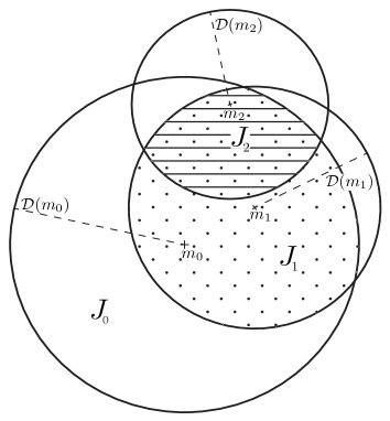
Figure 1: Illustration of our exact search for T-estimation. Along the three first iterations, the estimators $m_{i}$, $i=0,1,2$ are considered with associated radii $\mathcal{D}(m_{i})$ and the T-estimator belongs successively to $J_{i}$ where $J_{0}$ is $\bar{\mathcal{B}}(m_{0},\mathcal{D}(m_{0}))$, $J_{1}$ is the dotted and $J_{2}$ the hatched area.

Lemma 1.

For any point $m_{0}\in\left\{\left.1,\ldots,M\right.\right\}$, the T-estimator $\hat{m}$ belongs to $\bar{\mathcal{B}}(m_{0},\mathcal{D}(m_{0}))$.

Proof.

Suppose that there exists one point $m_{0}\in\left\{\left.1,\ldots,M\right.\right\}$ such that $\hat{m}$ does not belong to the closed ball of radius $\mathcal{D}(m_{0})$ centered at $m_{0}$. Then it does not belong to $\mathcal{R}_{m_{0}}$, and it follows that $\psi_{m_{0},\hat{m}}=m_{0}$. Hence $m_{0}$ belongs to $\mathcal{R}_{\hat{m}}$ leading to $\mathcal{D}(\hat{m})\geq d(\hat{m},m_{0})>\mathcal{D}(m_{0})$ which provides a contradiction with $\mathcal{D}(\hat{m})=\min_{m\in\left\{\left.1,\ldots,M\right.\right\}}\mathcal{D}(m)$. ∎

Corollary 1.

For any subset $J\subset\left\{\left.1,\ldots,M\right.\right\}$, the T-estimator $\hat{m}$ belongs to

$$\bigcap_{m\in J}\bar{\mathcal{B}}(m,\mathcal{D}(m))\enspace.$$

Proof.

The proof, illustrated by Figure 1, is straightforward using similar arguments as in Lemma 1. ∎

It follows that, starting from $m_{0}$, only a point inside $\bar{\mathcal{B}}(m_{0},\mathcal{D}(m_{0}))$ may be the T-estimator. If any point $m_{1}$ in this first ball satisfies $\mathcal{D}(m_{1})<\mathcal{D}(m_{0})$, by Lemma 1, the T-estimator will belong to $\bar{\mathcal{B}}(m_{0},\mathcal{D}(m_{0}))\bigcap\bar{\mathcal{B}}(m_{1},\mathcal{D}(m_{1}))$. Again, criterion $\mathcal{D}$ needs to be computed only for points inside this intersection. We keep intersecting balls $\bar{\mathcal{B}}(m,\mathcal{D}(m))$ until there are no more points with a value of $\mathcal{D}$ smaller than its running value. This approach provides an exact computation of the T-estimator.

At each step of the recursion, the current best point is denoted $m$ with associated value $\mathcal{D}(m)$ denoted by $\mathcal{D}$. The running intersection which contains the potentially better points than $m$ is denoted $J$ (this set does not contain $m$). The recursion stops when $J$ is empty. At a given step of the recursion, a point $j$ in $J$ is better than $m$ - and thus replaces it - if $\mathcal{D}(j)<\mathcal{D}$. In all cases, $j$ is removed from the set $J$. During the iteration, $|J|$ and $\mathcal{D}$ decrease ensuring that the algorithm stops. The last running $m$ is the T-estimator. The pseudo-code implementing the efficient and exact search of the T-estimator is provided by Algorithm 1.

Input: $m\in J=\left\{\left.1,\ldots,M\right.\right\}$

1 for $(j\neq m)$ do compute $\psi_{m,j}(\textbf{X}_{v})$

2 Compute $\mathcal{D}=\mathcal{D}(m)$ and set $J=\bar{\mathcal{B}}(m,\mathcal{D})\setminus\{m\}$

3while $(|J|>0)$ do

4       Set $\mathcal{D}_{tmp}=0$, select $j\in J$ and set $J=J\setminus\{j\}$

5      for $(k\neq j)$ do

6             Compute $\psi_{k,j}(\textbf{X}_{v})$ // if it has not been done yet

7            if $(\psi_{k,j}(\textbf{X}_{v})==k)$ then // $k\in\mathcal{R}_{j}$

8                   Set $\mathcal{D}_{tmp}=\max(\mathcal{D}_{tmp},d(j,k))$

9                  if $(\mathcal{D}_{tmp}>\mathcal{D})$ then break // break the for loop

10                  

11            

12       Set $m=j$, $\mathcal{D}=\mathcal{D}_{tmp}$ and $J=J\bigcap\bar{\mathcal{B}}(m,\mathcal{D})$

13 Return: $m$ // the T-estimator

14

Algorithm 1 Efficient and exact T-Hold-Out

Comments: This algorithm works for all the statistical frameworks of T-estimation, and does not depend on the considered robust test. The “for” loop is realized on all $k\not=j$, as $\mathcal{D}(k)$ depends on all points and not only on those in $J$. If there are $N$ points in the first ball, the number of computed tests is at most $O(N*M)$. Moreover, if the first ball is empty, i.e. if $\mathcal{D}(m)=0$, the algorithm stops immediately, returning $m$ for $\hat{m}$. In this case, the complexity of our algorithm is $O(M)$. Any preliminary estimator (maximum likelihood, least-squares, $L_{1}$-minimizer, etc.) may be a starting point of our algorithm. We hope that by beginning from a good preliminary estimator, there will be only few points in the first ball, resulting in less computations. The computation requires $O(M^{2})$ operations if $J$ decreases by only one point at each step of the recursion which happens only if the selected $j$ satisfies

$$\max_{k\in J}d(j,k)=\max_{k\neq l\in J}d(k,l)$$

at each iteration.

3.2 Fast algorithm for approximate T-Hold-Out

Assumption A ensures that as soon as the Hellinger distance between two estimators of $S$ is large enough, the probability that the robust test does not choose the best estimator is small. However, as shown in Lemma 1 of Le Cam (1973), when this distance is smaller than $c\,n^{-1/2}$, where $c$ is a small positive constant, the two corresponding probabilities cannot be separated by a test built on $n$ observations anymore. From this remark, we derive a lossy version from our efficient and exact algorithm. The main difference consists in ignoring points in $S$ as soon as their Hellinger distance to a previously considered one is smaller than a given threshold $\delta_{n}>0$.

We introduce this distance control at two steps of our efficient and exact algorithm. As the interior points of $\bar{\mathcal{B}}(m,\delta_{n})$ cannot be properly distinguished from $m$ by any test, the set $J$ becomes, at lines 1 and 1 of Algorithm 1, the intersection of rings instead of balls, obtained by removing from the original ball $\bar{\mathcal{B}}(m,\mathcal{D}(m))$ the ball $\bar{\mathcal{B}}(m,\delta_{n})$. In the same spirit, at line 1 of Algorithm 1, the current $k$, in the for loop, is considered if and only if its distance to $\mathcal{T}_{j}$ is larger than $\delta_{n}$, where $\mathcal{T}_{j}$ is made of the running $j$ and the further points which have been tested against $j$. The pseudo-code of this lossy version is provided by Algorithm 2 and illustrated by Figure 2.

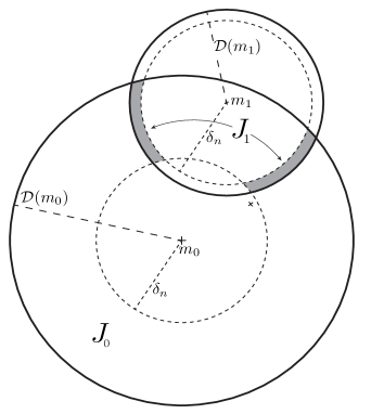
Figure 2: Illustration of the approximate T-estimation search: $J_{0}$ is a ring around $m_{0}$. The point following $m_{0}$ has changed with respect to Figure 1 as the previously selected $m_{1}$ is now inside $\bar{\mathcal{B}}(m_{0},\delta_{n})$. $J_{1}$ (in grey) appears as the intersection of two rings.

Input: $m\in J=\left\{\left.1,\ldots,M\right.\right\}$; $\delta_{n}>0$

1

2for $(j\neq m)$ do compute $\psi_{m,j}(\textbf{X}_{v})$

3 Compute $\mathcal{D}=\mathcal{D}(m)$ and set $J=\bar{\mathcal{B}}(m,\mathcal{D})\setminus\bar{\mathcal{B}}(m,\delta_{n})$

4while $(|J|>0)$ do

5       Set $\mathcal{D}_{tmp}=0$, select $j\in J$ and set $J=J\setminus\{j\}$

6      Define $\mathcal{T}_{j}=\{j\}$

7      for $(k\neq j)$ do

8            

9            if $(d(j,\mathcal{T}_{j})\leq\delta_{n})$ then next $k$ // next $k$ if distance is too small

10            

11            Set $\mathcal{T}_{j}=\mathcal{T}_{j}\cup\{k\}$

12            Compute $\psi_{k,j}(\textbf{X}_{v})$ // if it has not been done yet

13            if $(\psi_{k,j}(\textbf{X}_{v})==k)$ then // $k\in\mathcal{R}_{j}$

14                   Set $\mathcal{D}_{tmp}=\max(\mathcal{D}_{tmp},d(j,k))$

15                  if $(\mathcal{D}_{tmp}>\mathcal{D})$ then break // break the for loop

16                  

17            

18       Set $m=j$, $\mathcal{D}=\mathcal{D}_{tmp}$ and $J=J\bigcap\left[\bar{\mathcal{B}}(m,\mathcal{D})\setminus\bar{\mathcal{B}}(m,\delta_{n})\right]$

19 Return: $m$ // the approximate T-estimator

20

Algorithm 2 Approximate T-Hold-Out

4 Simulation protocol

In our simulations, we consider only the density estimation framework. This is motivated by the fact that likelihood ratio tests are not robust in this context, and we hoped to observe differences in terms of risk.

We considered $\textbf{X}=\left\{\left.X_{1},\ldots,X_{n}\right.\right\}$ i.i.d. random variables from an unknown density $s$ with respect to the Lebesgue measure on $\mathcal{X}=\mathbb{R}$ and, for a given proportion $p$ in $(0,1)$, we divide randomly X into $\textbf{X}_{t}=\left\{\left.X_{1},\ldots,X_{n_{1}}\right.\right\}$ and $\textbf{X}_{v}=\left\{\left.X_{n_{1}+1},\ldots,X_{n}\right.\right\}$, with $n_{1}=[pn]$ where $[x]$ is the integer part of $x$. Simulations were carried out with four sample sizes $n=100,250,500,1000$ and three different proportions $p=1/2,2/3,3/4$ using the two different robust tests (2) and (3). Our test functions $s$ vary in a subset $\mathcal{L}$ made of the densities $s_{1}$,…, $s_{28}$ of the R-package benchden which are in $L_{1}\cap L_{2}$ - to ensure that risks are computable. This set $\mathcal{L}$ is made of the densities $s_{i}$ for

$$i\in\left\{\left.1,\ldots,5,7,11,12,13,16,17,21,\ldots,27\right.\right\}.$$

We considered several estimator collections:

• $S_{R}$ made of regular histograms with bin number varying from 1 to $\lceil n_{1}/\log(n_{1})\rceil$ as described in Birgé and Rozenholc (2006);

• $S_{I}$ made of the maximum likelihood irregular histograms when the bin number only varies from 1 to $\min(100,\lceil n_{1}/\log(n_{1})\rceil)$ as described in Rozenholc et al. (2010);

• $S_{K}$ made of Gaussian kernel estimators with the varying bandwidths chosen as

  $$(\max[\textbf{X}_{t}]-\min[\textbf{X}_{t}])/2j\quad\mbox{ for }\quad j=1,\ldots,\lceil n_{1}/\log(n_{1})\rceil.$$

• $S_{P}$ made of parametric estimates obtained by moment’s method for the Gaussian, exponential, log-normal, chi-square, gamma and beta distributions together with a maximum likelihood estimate of the uniform distribution;

• $S_{C}=S_{R}\cup S_{I}$

• $S_{1}=S_{R}\cup S_{I}\cup S_{K}$;

• $S_{2}=S_{R}\cup S_{I}\cup S_{K}\cup S_{P}$.

The estimation accuracy of a given procedure $\tilde{s}$ has been evaluated using an empirical version of the risk $R_{s}(\tilde{s},\ell)=\mathbb{E}_{s}[\ell(\tilde{s},s)]$, obtained by generating $100$ $n$-samples $\textbf{X}^{(j)}$, $1\leq j\leq 100$, of density $s$:

$$\bar{R}_{s}(\tilde{s},\ell)=\frac{1}{100}\sum_{j=1}^{100}\ell(\tilde{s}[\textbf{X}^{(j)}],s)\enspace,$$

where $\ell(t,u)$ is either $h^{2}(t,u)$ or $\|t-u\|_{q}^{q}$, for $q=1,2$.

In order to compare two procedures $\tilde{t}_{1}$ and $\tilde{t}_{2}$, we introduce the normalized $\log_{2}$-ratio of their empirical risks, namely:

$$\bar{W}_{s}(\tilde{t}_{1},\tilde{t}_{2})=\frac{1}{r}\log_{2}\frac{\bar{R}_{s}(\tilde{t}_{1},\ell)}{\bar{R}_{s}(\tilde{t}_{2},\ell)}=\log_{2}\bar{R}_{s}^{1/r}(\tilde{t}_{1},\ell)-\log_{2}\bar{R}_{s}^{1/r}(\tilde{t}_{2},\ell)\enspace,$$

where $r$ is equal to $q$ for $L_{q}$ losses and 2 for the Hellinger loss. The aim of the normalization by $r$ is to provide an easier comparison of $\bar{W}_{s}$ when the loss changes. In our empirical study, procedure $\tilde{t}_{2}$ is thus considered better in terms of risk than $\tilde{t}_{1}$ for a given loss function $\ell$ if the values of $\bar{W}_{s}(\tilde{t}_{1},\tilde{t}_{2})$ are positive when the density $s$ varies.

We compared the four hold-out methods described above: T-estimation with the tests given by (2) and (3), LS and KL. We first computed $\hat{s}_{m}[\textbf{X}_{t}]$ for all $m\in\cal M$, and then selected $\hat{m}$ minimizing the respective HO criterion resulting in $\hat{m}_{T1}$, $\hat{m}_{T2}$, $\hat{m}_{LS}$ and $\hat{m}_{KL}$, providing $\tilde{s}$ as either $\hat{s}_{\hat{m}}[\textbf{X}_{t}]$ or $\hat{s}_{\hat{m}}[\textbf{X}]$. As $\hat{m}$ depends on the chosen proportion $p$, in order to explicitly specify the dependency of $\hat{m}$ with respect to this parameter, we will use the following notations $\hat{s}_{\hat{m}[p]}[\textbf{X}_{t}]$ or $\hat{s}_{\hat{m}[p]}[\textbf{X}]$ when needed. In Algorithms 1 and 2, the input $m$ has been set to $\hat{m}_{LS}$ and $j=\arg\max_{k\in J}d(k,m)$, at line 1. In Algorithm 2, we fixed $\delta_{n}=1/\sqrt{|\textbf{X}_{v}|}$ as a lower bound for the Hellinger distance between distinguishable probabilities, following Le Cam (1973).

Moreover, we also considered some calibrated estimation procedures which choose $m$ in some particular families. These are not direct competitors with the T-estimation as they cannot deal with general families $S$ but provide a good benchmark in terms of risk:

• for $S_{R}$, $S_{I}$, $S_{C}$, the penalized maximum likelihood estimators, denoted $\tilde{s}_{\rm pen}$ introduced in Birgé and Rozenholc (2006); Rozenholc et al. (2010) and implemented in the R-package histogram,

• for $S_{K}$, the ${L}_{1}$-version of the procedure introduced in Goldenshluger and Lepski (2011), denoted $\tilde{s}_{GL}$.

For fairness, we applied these calibrated estimation procedures in their original setting which use the full sample replacing $n_{1}$ by $n$ in the definition of $S_{R}$ and $S_{K}$.

Finally, for the family $S_{K}$, we considered some bandwidth selectors (namely nrd, ucv, bcv, SJ) implemented in the density generic function available in R , providing some well-known estimators $\tilde{s}_{nrd}$, $\tilde{s}_{bcv}$, $\tilde{s}_{ucv}$, $\tilde{s}_{SJ}$ of the density which are not chosen in $S$ (Silverman, 1986; Sheather and Jones, 1991; Scott, 1992).

The R-package Density.T.HoldOut is a ready-to-use software that implements our algorithms in the density framework. The main function - called DensityTestim - receives as input a sample X and a family of estimators and returns the selected estimator. The previously described families are available and can be extended or adapted by the user (default family is $S_{2}$). Other important input arguments are parameters $p$, $\theta$ and the starting point (default values are $p=1/2$ , $\theta=1/4$ and $\hat{m}_{LS}$). This function implements the exact and lossy algorithms, through the numeric csqrt (default value 1) which controls $\delta_{n}={\tt csqrt}/\sqrt{|\textbf{X}_{v}|}$ in Algorithm 2. The robust test might be the one defined by (2) setting test=’birge’ (default), or by (3) setting test=’baraud’. The resulting estimator is either built with $\textbf{X}_{t}$ (last=’training’) or X (last=’full’, default).

5 Simulation results

This section, made using Algorithm 1, is devoted to the study of the quality of the T-hold-out. We illustrate our results showing boxplots of $\bar{W}_{s}(\tilde{t}_{1},\tilde{t}_{2})$ for all 18 densities $s\in\mathcal{L}$, various choices of estimators $\tilde{t}_{1}$ and $\tilde{t}_{2}$ and for different collections of estimators $S$, as described in the previous section. We begin by investigating how parameter $\theta$ influences the THO procedure deduced from (2). Then we show that the two robust procedures derived from (2) and (3) have similar behavior in terms of risk, and therefore pursue using the first one only. After studying how $p$ influences the quality of estimation, we provide two main comparison types. First we look at HO methods which select among a family of points using the validation sample. Then we compare the THO against some density estimation methods, which are not necessarily selection procedures anymore. In this subsection, we divide the presentation between calibrated selection procedures build directly on the full sample and some selectors of the bandwidth obtained using asymptotic derivation of the risk for some specific loss.

5.1 Influence of $\theta$

The robustness of the procedure build using (2) is controlled through the parameter $\theta<1/2$ (see Eq. 2), the KLHO corresponding to $\theta=0$ (no robustness). We computed the empirical risk using the THO procedure with $\theta=1/16,1/8,1/4,3/8,7/16$, and $n=100,250,500,1000$. We observed that $\theta$ has little influence in terms of risk ($\theta=1/16$ being slightly worse) and decided to pursue the empirical study with $\theta=1/4$.

5.2 Influence of the robust test

As we dispose of two robust tests to proceed the THO, we compare the two corresponding strategies in Figure 3 using $\tilde{t}_{1}=\hat{s}_{\hat{m}_{T1}[p]}[\textbf{X}_{t}]$ and $\tilde{t}_{2}=\hat{s}_{\hat{m}_{T2}[p]}[\textbf{X}_{t}]$ for $p=1/2$, $2/3$ and $3/4$ (each value corresponding to one subfigure below). For a fixed $n$, there are $18\times 6$ ratios obtained when both the density and the collection of estimators vary.

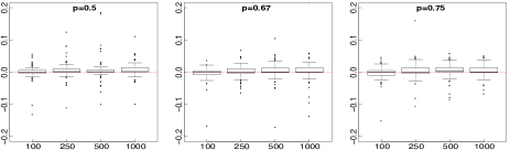
Figure 3: From left to right, normalized $\log_{2}$-ratio of the empirical risks $\bar{W}_{s}(\hat{s}_{\hat{m}_{T1}[p]}[\textbf{X}_{t}],\hat{s}_{\hat{m}_{T2}[p]}[\textbf{X}_{t}])$ for the Hellinger loss for $p=1/2$, $2/3$ and $3/4$. Each subfigure shows the boxplot for $n$ equals 100, 250, 500 and 1000. The horizontal red dotted line provides the reference value 0.

Surprisingly the two procedures behave very similarly in all settings, and only few differences can be observed in terms of Hellinger risk (generally less than 2%). We therefore pursue our empirical study with the procedure derived from (2), and from now on we denote $\hat{m}_{T}$ instead of $\hat{m}_{T1}$, when no confusion is possible.

5.3 Influence of $p$

We examine the dependence of the THO with respect to $p$, the proportion of the initial sample dedicated to building the estimators, using the Hellinger risk.

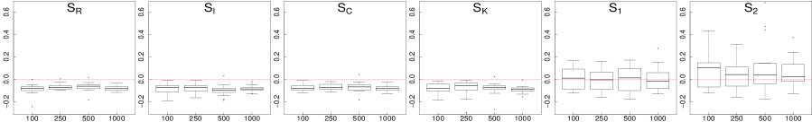
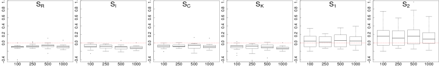
Figure 4: From left to right, normalized $\log_{2}$-ratio of the empirical risks $\bar{W}_{s}(\hat{s}_{\hat{m}_{T}[2/3]}[\textbf{X}_{t}],\hat{s}_{\hat{m}_{T}[1/2]}[\textbf{X}_{t}])$ (upper line) and $\bar{W}_{s}(\hat{s}_{\hat{m}_{T}[3/4]}[\textbf{X}_{t}],\hat{s}_{\hat{m}_{T}[1/2]}[\textbf{X}_{t}])$ (bottom line) for the Hellinger loss, using collections $S_{R}$, $S_{I}$, $S_{C}$, $S_{K}$, $S_{1}$ and $S_{2}$. Each subfigure shows the boxplot for $n$ equals 100, 250, 500 and 1000. The horizontal red dotted line provides the reference value 0.

Figure 4 is built using $\tilde{t}_{1}=\hat{s}_{\hat{m}_{T}[p]}[\textbf{X}_{t}]$ for $p$ equals 2/3 (upper line), 3/4 (bottom line) and $\tilde{t}_{2}=\hat{s}_{\hat{m}_{T}[1/2]}[\textbf{X}_{t}]$. We observe two different behaviors for families $S_{R}$, $S_{I}$, $S_{C}$ and $S_{K}$ on the one hand and for $S_{1}$ and $S_{2}$ on the other hand. For the first families $p=2/3$ or $3/4$ is better than $p=1/2$. For the second ones $p=2/3$ seems equivalent to $p=1/2$ but $p=3/4$ is worst than $p=1/2$. Hence we consider preferable to use $p=2/3$, which makes the best compromise for all families.

5.4 Comparing Hold-Out methods

Hold-out procedures are universal since they do not depend on the choice of family $S$. They can be seen as methods that choose among some family of fixed points. Setting $p=2/3$, we compare the THO to the KLHO and LSHO introduced in Section 1.2 using each of the 6 estimator collections described in Section 4.

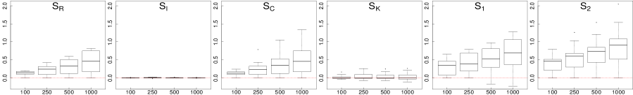
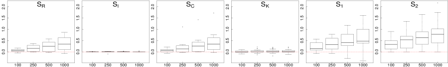
Figure 5: From left to right, normalized $\log_{2}$-ratio of the empirical risks $\bar{W}_{s}(\hat{s}_{\hat{m}_{KL}}[\textbf{X}_{t}],\hat{s}_{\hat{m}_{T}}[\textbf{X}_{t}])$ for $p=2/3$, using collections $S_{R}$, $S_{I}$, $S_{C}$, $S_{K}$, $S_{1}$ and $S_{2}$. Upper line, using Hellinger loss, bottom line using $L_{1}$ loss. See Figure 4 for more details.

Figure 5 is built using $\tilde{t}_{1}=\hat{s}_{\hat{m}_{KL}}[\textbf{X}_{t}]$ and $\tilde{t}_{2}=\hat{s}_{\hat{m}_{T}}[\textbf{X}_{t}]$ considering Hellinger (upper line) and $L_{1}$ (bottom line) losses. In all cases, the median and most of the distribution are positive, meaning that the THO outperforms the KLHO estimator. For collections $S_{I}$ and $S_{K}$, empirical risks for both losses are similar, with $\bar{W}_{s}(\hat{s}_{\hat{m}_{KL}}[\textbf{X}_{t}],\hat{s}_{\hat{m}_{T}}[\textbf{X}_{t}])$ being respectively larger than -0.01 (except for the uniform density) for $S_{I}$, and -0.2 for $S_{K}$. When $n$ grows, while for $S_{I}$ and $S_{K}$ the ratio remains stable, it increases for all other families in favor of the THO. Moreover when going from collection $S_{1}$ to $S_{2}$, that is adding the parametric collection $S_{P}$, we observe that the already good performance of the THO improves. We therefore suspect that the THO chooses the parametric estimator more often than KLHO when facing the corresponding densities.

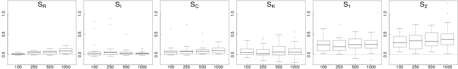
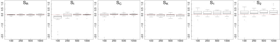
Figure 6: From left to right, normalized $\log_{2}$-ratio of the empirical risks $\bar{W}_{s}(\hat{s}_{\hat{m}_{LS}}[\textbf{X}_{t}],\hat{s}_{\hat{m}_{T}}[\textbf{X}_{t}])$ for $p=2/3$, using collections $S_{R}$, $S_{I}$, $S_{C}$, $S_{K}$, $S_{1}$ and $S_{2}$. Upper line, using Hellinger loss, bottom line using $L_{2}$ loss. See Figure 4 for more details.

Figure 6 is built using $\tilde{t}_{1}=\hat{s}_{\hat{m}_{LS}}[\textbf{X}_{t}]$ and $\tilde{t}_{2}=\hat{s}_{\hat{m}_{T}}[\textbf{X}_{t}]$ considering Hellinger (upper line) and $L_{2}$ (bottom line) losses. The THO performs better than the LSHO estimator for all collections except for the collection $S_{I}$ when $n=100$. For the larger collections $S_{1}$ and $S_{2}$, the THO outperforms the LSHO. However, as $n$ grows, we observe that the relative quality of the two procedures remain stable.

5.5 Comparing final strategies for T-Hold-Out

Here, we investigate whether $\hat{s}_{\hat{m}_{T}}[\textbf{X}_{t}]$ or $\hat{s}_{\hat{m}_{T}}[\textbf{X}]$ performs better. For this purpose, we study the Hellinger risk of $\hat{s}_{\hat{m}_{T}}[\textbf{X}]$ when $p$ varies. Figure 7 is built using $\tilde{t}_{1}=\hat{s}_{\hat{m}_{T}[p]}[\textbf{X}]$ for $p$ equals 2/3 (upper line), 3/4 (bottom line) and $\tilde{t}_{2}=\hat{s}_{\hat{m}_{T}[1/2]}[\textbf{X}]$. We observe that against $p=2/3$ or $p=3/4$, the value $p=1/2$ provides better results for the large families $S_{1}$ and $S_{2}$ while for the small families the results are more balanced. Hence we consider preferable to make use of this strategy with $p=1/2$.

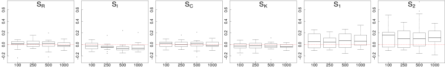
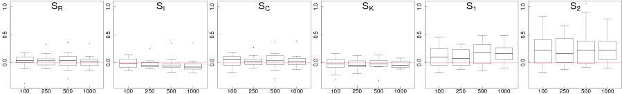
Figure 7: From left to right, normalized $\log_{2}$-ratio of the empirical risks $\bar{W}_{s}(\hat{s}_{\hat{m}_{T}[2/3]}[\textbf{X}],\hat{s}_{\hat{m}_{T}[1/2]}[\textbf{X}])$ (upper line) and $\bar{W}_{s}(\hat{s}_{\hat{m}_{T}[3/4]}[\textbf{X}],\hat{s}_{\hat{m}_{T}[1/2]}[\textbf{X}])$ (bottom line) for the Hellinger loss, using collections $S_{R}$, $S_{I}$, $S_{C}$, $S_{K}$, $S_{1}$ and $S_{2}$. See Figure 4 for more details.

We now compare the Hellinger risks of $\hat{s}_{\hat{m}_{T}[2/3]}[\textbf{X}_{t}]$ - which appeared as the best competitor in Section 5.3 - and $\hat{s}_{\hat{m}_{T}[1/2]}[\textbf{X}]$. Figure 8 is built using $\tilde{t}_{1}=\hat{s}_{\hat{m}_{T}[1/2]}[\textbf{X}]$ and $\tilde{t}_{2}=\hat{s}_{\hat{m}_{T}[2/3]}[\textbf{X}_{t}]$. We observe that the strategy $\hat{s}_{\hat{m}_{T}[1/2]}[\textbf{X}]$ is preferable, since its median (and even most of its distribution) is negative in all considered settings. It should be noticed that our simulations show that, more than the value of $p$, it is the use of X instead of $\textbf{X}_{t}$ which has the larger influence on the final risk.

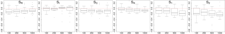
Figure 8: From left to right, normalized $\log_{2}$-ratio of the empirical risks $\bar{W}_{s}(\hat{s}_{\hat{m}_{T}[1/2]}[\textbf{X}],\hat{s}_{\hat{m}_{T}[2/3]}[\textbf{X}_{t}])$ for Hellinger loss, using collections $S_{R}$, $S_{I}$, $S_{C}$, $S_{K}$, $S_{1}$ and $S_{2}$. See Figure 4 for more details.

5.6 T-Hold-Out against dedicated estimation procedures

We now compare the THO competitor $\hat{s}_{\hat{m}_{T}[1/2]}[\textbf{X}]$ against the so-called dedicated methods. Figure 9 is built using $\tilde{t}_{1}=\tilde{s}[\textbf{X}]$ ($\tilde{s}$ being either $\tilde{s}_{\rm pen}$ or $\tilde{s}_{GL}$) and $\tilde{t}_{2}=\hat{s}_{\hat{m}_{T}[1/2]}[\textbf{X}]$ considering Hellinger (upper line) and $L_{1}$ (bottom line) losses. We observe that the THO is slightly worse than a well-calibrated procedure for histograms but outperforms the $L_{1}$-version of the Goldenshluger-Lepski procedure.

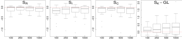
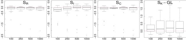
Figure 9: From left to right, normalized $\log_{2}$-ratio of the empirical risks $\bar{W}_{s}(\tilde{s}[\textbf{X}],\hat{s}_{\hat{m}_{T}[1/2]}[\textbf{X}])$ using collections $S_{R}$, $S_{I}$, $S_{C}$ and $S_{K}$ with Hellinger (upper line) and $L_{1}$ (bottom line) losses. For the 3 first collections $\tilde{s}$ is $\tilde{s}_{\rm pen}$ and $\tilde{s}_{GL}$ for $S_{K}$. Each subfigure shows the boxplot for $n$ equals 100, 250, 500 and 1000. The horizontal red dotted line provides the reference value 0.

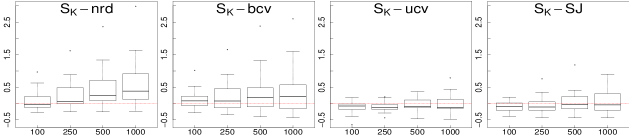
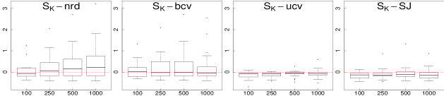
Figure 10: From left to right, normalized $\log_{2}$-ratio of the empirical risks $\bar{W}_{s}(\tilde{s}[\textbf{X}],\hat{s}_{\hat{m}_{T}[1/2]}[\textbf{X}])$ for collection $S_{K}$. The 3 first competitors $\tilde{s}$ are the kernel estimators with respective bandwidth provided by the bandwidth selectors $nrd$, $bcv$, $ucv$ and $SJ$ as defined in the function density of the stats package of R. Upper line, using Hellinger loss, bottom line using $L_{1}$ loss. See Figure 4 for more details.

For the sake of completeness, we also provide in Figure 10 the comparison between the THO and well-known estimators of the density derived from bandwidth selectors available in the density generic function of R. We observe that $\tilde{s}_{ucv}$ and $\tilde{s}_{SJ}$ perform well (particularly for the $L_{1}$-loss), whereas the THO outperforms $\tilde{s}_{nrd}$ and $\tilde{s}_{bcv}$.

6 Empirical complexity of the exact algorithm

To evaluate the complexity of our algorithms let us denote by $N$ the number of tests needed in the computation of the THO for each generated sample of our simulations. As $N$ is between $M-1$ and $M(M-1)/2$, we define the so-called “THO complexity” as the ratio of $N-M+1$ over its maximal value, that is

$$\frac{2(N-M+1)}{(M-1)(M-2)}\enspace.$$ (6)

For any run, this ratio belongs to $[0,1]$ by construction. For each fixed $n$, we get a global sample of size 10800 corresponding to “18 densities” times “6 families” times “100 simulations”. Figure 11 shows the empirical cumulative distribution function (CDF) of the latter sample with the quantiles 0.75, 0.9 and 0.95, for both tests (2) and (3). We observe from this figure that in both cases the complexity of our algorithm tends to improve with $n$. Moreover, 75% of the THO complexities are smaller than 0.1 for $n$ equals 250, 500 and 1000 and 95% are smaller than 0.4 for all values of $n$. The THO complexity using (3) is slightly smaller. However the comparison of two estimators in (3) requires the computation of one integral to compute the difference of squared Hellinger distances involving the middle point. From a practical point-of-view, we indeed observed that using the test (3) is more CPU time-consuming. Since both strategies have similar THO complexity, we pursue our study again using the procedure derived from (2) only.

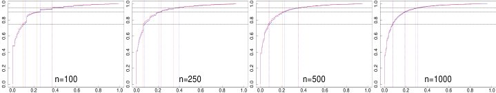
Figure 11: From left to right, the CDF for $n=100$, 250, 500 and 1000 of the THO complexity using Algorithm 1 in plain line: procedure derived from (2) in blue and from (3) in red. The horizontal black dotted lines provide the values 0.75, 0.9 and 0.95 and the vertical dotted lines their respective quantiles using the respective colors.

In order to complete this study of the complexity we focused on the two collections $S_{R}$ and $S_{K}$ for which the number of estimators depends on $n$ as $M=\lceil n_{1}/\log(n_{1})\rceil$. Having in mind that $N$ is not smaller than $M-1$ and not larger than $M(M-1)/2$, we assumed $N$ to be of order $(M-1)^{\beta}$ with $\beta$ in $[1,2]$. For each density and each value of $n$, we compute the average of $\log(N)$ over the 100 runs. In Figure 12 these average values are drawn versus $\log(M-1)$ for the two collections and for each density.

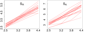
Figure 12: Graphs of $\log(N)$ versus $\log(M-1)$ for each density when using the collections $S_{R}$ (left) and $S_{K}$ (right).

As Figure 12 exhibits mostly linear behaviors, we computed the slope in the linear model of $\log(N)$ versus $\log(M-1)$ as an estimator of $\beta$ when $n_{1}$ varies. We observe that this estimator concentrates around respectively 1.2 and 1.4 for the collections $S_{R}$ and $S_{K}$ providing a good indicator that our algorithm is typically sub-quadratic. The larger value of $\beta$ for the collection $S_{K}$ may be explained by the fact that, for our set of bandwidths, the kernel estimators may be very similar, inducing a slow decrease of the running intersection $J$ in Algorithm 1.

7 Study of the approximate T-Hold-Out

We provide a comparison of the estimators selected using Algorithms 1 and 2 respectively, that is the exact T-estimator and its approximate version (denoted here by $\hat{m}_{T}^{g}$) computed with $\delta_{n}={c}/\sqrt{|\textbf{X}_{v}|}$ for different values of $c$. We compare these estimators using the two strategies based on $\textbf{X}_{t}$ and X.

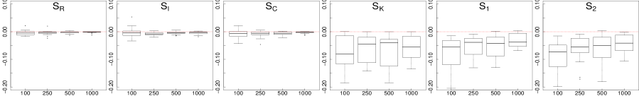
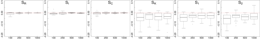
Figure 13: From left to right, normalized $\log_{2}$-ratio of the empirical risks $\bar{W}_{s}(\hat{s}_{\hat{m}_{T}}[\textbf{X}_{t}],\hat{s}_{\hat{m}_{T}^{g}}[\textbf{X}_{t}])$ (upper line) and $\bar{W}_{s}(\hat{s}_{\hat{m}_{T}}[\textbf{X}],\hat{s}_{\hat{m}_{T}^{g}}[\textbf{X}])$ using $c=1$ (bottom line) for the Hellinger loss, using collections $S_{R}$, $S_{I}$, $S_{C}$, $S_{K}$, $S_{1}$ and $S_{2}$. See Figure 4 for more details.

Figure 13 is built using $\tilde{t}_{1}=\hat{s}_{\hat{m}_{T}}[\textbf{X}_{t}]$ and $\tilde{t}_{2}=\hat{s}_{\hat{m}_{T}^{g}}[\textbf{X}_{t}]$ with $p=2/3$ on the upper line and using $\tilde{t}_{1}=\hat{s}_{\hat{m}_{T}}[\textbf{X}]$ and $\tilde{t}_{2}=\hat{s}_{\hat{m}_{T}^{g}}[\textbf{X}]$ with $p=1/2$ on the bottom line. As expected, the exact THO is better in terms of risk. For histogram families, the degradation of the Hellinger risk is negligible. For families $S_{K}$, $S_{1}$ and $S_{2}$, we observe that the risk increases not more than 20% in most of the cases ($y$-axis reference value equals to -0.13). The empirical cumulative distribution function (CDF) of the complexity ratio defined in (6) is shown in Figure 14, for both tests, for comparison with Figure 11. Clearly the CDFs of the lossy version are more concentrated around 0, showing a significant gain in terms of complexity when using Algorithm 2 (quantiles are divided by more than 2.5).

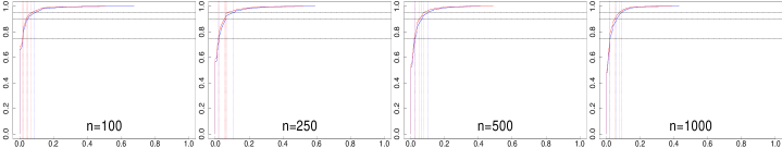
Figure 14: From left to right, the CDF for $n=100$, 250, 500 and 1000 of the THO complexity in plain line using Algorithm 2 with $c=1$. See Figure 11 for more details.

A further study, using $c=2$ in the approximate algorithm, shows that the risk increases up to 75% in most of the cases and does not offer a good trade-off between complexity and accuracy.

8 Conclusion

We introduce an efficient and exact algorithm, together with an approximate version, for T-estimation in the context of hold-out. We study the performances of this T-hold-out in the density framework using two different robust tests. Calibration study shows that, when building the final estimate only with the training sample, a good choice of the ratio between training and validation sample sizes is $p=2/3$. However, risks can be improved using the full sample to build the final estimate when using $p=1/2$. Our procedure is competitive compared to classical hold-out derived from Kullback-Leibler or least-squares contrasts. It still behaves well against model selection procedures derived from a calibrated penalized contrast for histogram selection, and against most of the bandwidth selectors for kernel estimators. Empirically, we observe that this algorithm improves clearly the combinatorial complexity. Moreover, it can be speeded up thanks to our proposed lossy version, which offers the expected trade-off between complexity and estimation quality. Finally, the two THO strategies are very similar in terms of Hellinger risk and THO complexity, but we recommend to proceed the THO procedure based on (2) since it is less time-consuming.

References

- Arlot and Lerasle (2014) S. Arlot and M. Lerasle. Why V = 5 is enough in V -fold cross-validation. arXiv:1210.5830v2, 2014.
- Baraud (2011) Y. Baraud . Estimator selection with respect to Hellinger-type risks. Probab. Theory Related Fields, 151:353–401, 2011.
- Baraud and Birgé (2009) Y. Baraud and L. Birgé. Estimating the intensity of a random measure by histogram type estimators. Probab. Theory Related Fields, 143:239–284, 2009.
- Bartlett et al. (2002) P. Bartlett, S. Boucheron, and G. Lugosi. Model selection and error estimation. Machine Learning, 48:85–113, 2002.
- Berlinet and Devroye (1994) A. Berlinet and L. Devroye. A comparison of kernel density estimates. Publications de l’Institut de Statistique de l’Universite de Paris, 38(3):3–59, 1994.
- Birgé (1983) L. Birgé. Approximation dans les espaces métriques et theorie de l’estimation. Z. Wahrscheinlichkeitstheorie verw. Geb., 65:181–237, 1983.
- Birgé (1984a) L. Birgé. Sur un theorème de minimax et son application aux tests. Probab. Math. Statist., 3:259–282, 1984a.
- Birgé (1984b) L. Birgé. Stabilité et instabilité du risque minimax pour des variables indépendantes équidistribuées. Ann. Inst. H. Poincaré Sect. B, 20:201–223, 1984b.
- Birgé (2006) L. Birgé. Model selection via testing: an alternative to (penalized) maximum likelihood estimators. Ann. Institut Henri Poincare, Probab. et Statist., 42:273–325, 2006.
- Birgé (2007) L. Birgé. Model selection for Poisson Processes. Asymptotic: Particles, processes and inverse problems, Festschrift for Piet Groeneboom (E. Cator, G. Jongbloed, C. Kraaikamp, R. Lopuhaä and J. Wellner, eds), IMS Lecture Notes – Monograph Series 55:32–64, 2007.
- Birgé (2013a) L. Birgé. Robust tests for Model Selection. From Probability to Statistics and Back: High-Dimensional Models and Processes – A Festschrift in Honor of Jon A. Wellner (M.Banerjee, F. Bunea, J. Huang, V. Koltchinskii and M. Mathuis,eds), IMS Collections – Volume 9:47–64, 2013a.
- Birgé (2013b) L. Birgé. Model Selection for density estimation with -loss. Probab. Theory Related Fields, pages 1–42, 2013b.
- Birgé and Massart (1993) L. Birgé and P. Massart. Rates of convergence for minimum contrast estimators. Probab. Theory Related Fields, 97:113–150, 1993.
- Birgé and Rozenholc (2006) L. Birgé and Y. Rozenholc. How many bins should be put in a regular histogram. ESAIM Probab. Statist., 10:24–45, 2006.
- Blanchard and Massart (2006) G. Blanchard and P. Massart. Discussion: Local rademacher complexities and oracle inequalities in risk minimization. Ann. Statist., 34(6):2664–2671, 2006.
- Devroye and Lugosi (2001) L. Devroye and G. Lugosi. Combinatorial Methods in Density Estimation. Springer-Verlag, New York, 2001.
- Goldenshluger and Lepski (2011) A. Goldenshluger and O. Lepski. Bandwidth selection in kernel density estimation: oracle inequalities and adaptive minimax optimality. Ann. Statist., 39(3):1608–1632, 2011.
- Juditsky and Nemirovski (2000) A. Juditsky and A. Nemirovski. Functional aggregation for nonparametric estimation. Ann. Statist., 28:681–712, 2000.
- Larson (1931) S. C. Larson. The shrinkage of the coefficient of multiple correlation. J. Edic. Psychol., 22:45–55, 1931.
- Le Cam (1973) L. M. Le Cam. Convergence of estimates under dimensionality restrictions. Ann. Statist., 1:38–55, 1973.
- Lugosi and Nobel (1999) G. Lugosi and A.B. Nobel. Adaptive model selection using empirical complexities. Ann. Statist., 27(6):1830–1864, 1999.
- Mildenberger and Weinert (2012) T. Mildenberger and H. Weinert. The benchden package: Benchmark densities for nonparametric density estimation. Journal of Statistical Software, 46(14):1–14, 2012.
- Nemirovski (2000) A. Nemirovski. Topics in Non-Parametric Statistics. Lecture on Probability Theory and Statistics. Ecole d’Eté de Probabilités de Saint-Flour XXVIII - 1998 (P. Bernard, ed.) Lecture Notes in Math. Springer, Berlin, 2000.
- Rigollet and Tsybakov (2007) P. Rigollet and A. B. Tsybakov. Linear and convex aggregation of density estimators. Mathematical Methods of Statistics, 16(3):260–280, 2007.
- Rozenholc et al. (2010) Y. Rozenholc, T. Mildenberger, and U. Gather. Combining regular and irregular histograms by penalized likelihood. Computational Statistics and Data Analysis, 54(12):3313–3323, 2010.
- Sart (2011) M. Sart. Model selection for Poisson processes with covariates. arXiv:1112.5634, 2011.
- Sart (2012) M. Sart. Estimation of the transition density of a Markov chain. Ann. Inst. Henri Poincaré Probab. et Statis. (to appear), 2012.
- Sart (2013) M. Sart. Robust estimation on a parametric model with tests. http://arxiv.org/abs/1308.2927v2, 2013.
- Scott (1992) D.W. Scott. Multivariate Density Estimation: Theory, Practice, and Visualization. Wiley, 1992.
- Sheather and Jones (1991) S. J. Sheather and M. C. Jones. A reliable data-based bandwidth selection method for kernel density estimation. J. Roy. Statist. Soc. Ser. B., 53:683–690, 1991.
- Silverman (1986) B. W. Silverman. Density Estimation. London: Chapman and Hall, 1986.
- Wegkamp (2003) M. Wegkamp. Model selection in nonparametric regression. Ann. Statist., 31(1):252–273, 2003.