Abstract

This text is about the mathematical use of certain divergent power series.

The first part is an introduction to $1$-summability. The definitions rely on the formal Borel transform and the Laplace transform along an arbitrary direction of the complex plane. Given an arc of directions, if a power series is $1$-summable in that arc, then one can attach to it a Borel-Laplace sum, i.e. a holomorphic function defined in a large enough sector and asymptotic to that power series in Gevrey sense.

The second part is an introduction to Écalle’s resurgence theory. A power series is said to be resurgent when its Borel transform is convergent and has good analytic continuation properties: there may be singularities but they must be isolated. The analysis of these singularities, through the so-called alien calculus, allows one to compare the various Borel-Laplace sums attached to the same resurgent $1$-summable series. In the context of analytic difference-or-differential equations, this sheds light on the Stokes phenomenon.

A few elementary or classical examples are given a thorough treatment (the Euler series, the Stirling series, a less known example by Poincaré). Special attention is devoted to non-linear operations: $1$-summable series as well as resurgent series are shown to form algebras which are stable by composition. As an application, the resurgent approach to the classification of tangent-to-identity germs of holomorphic diffeomorphisms in the simplest case is included. An example of a class of non-linear differential equations giving rise to resurgent solutions is also presented. The exposition is as self-contained as can be, requiring only some familiarity with holomorphic functions of one complex variable.

This text grew out of a course given in a CIMPA school in Lima in 2008 and further courses taught at the Scuola Normale Superiore di Pisa between 2008 and 2010. We tried to make it as self-contained as possible, so that it can be used with undergraduate students, assuming only on their part some familiarity with holomorphic functions of one complex variable. The first part of the text (Sections 1–17) is an introduction to $1$-summability. The second part (Sections 18–37) is an introduction to Écalle’s resurgence theory.

Throughout the text, we use the notations

$$\mathbb{N}=\{0,1,2,\ldots\},\qquad\mathbb{N}^{*}=\{1,2,3,\ldots\}$$

for the set of non-negative integers and the set of positive integers.

Introduction

1 Prologue

1.1  At the beginning of the second volume of his New methods of celestial mechanics [Po94], H. Poincaré dedicates two pages to elucidating “a kind of misunderstanding between geometers and astronomers about the meaning of the word convergence”. He proposes a simple example, namely the two series

$$\sum\frac{1000^{n}}{n!}\quad\textrm{and}\quad\sum\frac{n!}{1000^{n}}.$$ (1)

He says that, for geometers (i.e. mathematicians), the first one is convergent because the term for $n=1.000.000$ is much smaller than the term for $n=999.999$, whereas the second one is divergent because the general term is unbounded (indeed, the $(n+1)$-th term is obtained from the $n$th one by multiplying either by $1000/n$ or by $n/1000$). On the contrary, according to Poincaré, astronomers will consider the first series as divergent because the general term is an increasing function of $n$ for $n\leq 1000$, and they will consider the second one as convergent because the first $1000$ terms decrease rapidly.

He then proposes to reconcile both points of view by clarifying the role that divergent series (in the sense of geometers) can play in the approximation of certain functions. He mentions the example of the classical Stirling series, for which the absolute value of the general term is first a decreasing function of $n$ and then an increasing function; this is a divergent series and still, Poincaré says, “when stopping at the least term one gets a representation of Euler’s gamma function, with greater accuracy if the argument is larger”. This is the origin of the modern theory of asymptotic expansions.

1.2  In this text we shall focus on formal series given as power series expansions, like the Stirling series for instance, rather than on numerical series. Thus, we would rather present Poincaré’s simple example (1) in the form of two formal series

$$\sum_{n\geq 0}\frac{1000^{n}}{n!}t^{n}\quad\textrm{and}\quad\sum_{n\geq 0}\frac{n!}{1000^{n}}t^{n},$$ (2)

the first of which has infinite radius of convergence, while the second has zero radius of convergence. For us, divergent series will usually mean a formal power series with zero radius of convergence.

Our first aim in this text is to discuss the Borel-Laplace summation process as a way of obtaining a function from a (possibly divergent) formal series, the relation between the original formal series and this function being a particular case of asymptotic expansion of Gevrey type. For instance, this will be illustrated on Euler’s gamma function and the Stirling series (see Section 11). But we shall also describe in this example and others the phenomenon for which J. Écalle coined the name resurgence at the beginning of the 1980s and give a brief introduction to this beautiful theory.

2 An example by Poincaré

Before stating the basic definitions and introducing the tools with which we shall work, we want to give an example of a divergent formal series $\tilde{\phi}(t)$ arising in connection with a holomorphic function $\phi(t)$ (later on, we shall come back to this example and see how the general theory helps to understand it). Up to changes in the notation this example is taken from Poincaré’s discussion of divergent series, still at the beginning of [Po94].

Fix $w\in\mathbb{C}$ with $0<|w|<1$ and consider the series of functions of the complex variable $t$

$$\phi(t)=\sum_{k\geq 0}\phi_{k}(t),\qquad\phi_{k}(t)=\frac{w^{k}}{1+kt}.$$ (3)

This series is uniformly convergent in any compact subset of $U=\mathbb{C}^{*}\setminus\big{\{}-1,-\frac{1}{2},-\frac{1}{3},\ldots\big{\}}$, as is easily checked, thus its sum $\phi$ is holomorphic in $U$.

We can even check that $\phi$ is meromorphic in $\mathbb{C}^{*}$ with a simple pole at every point of the form $-\frac{1}{k}$ with $k\in\mathbb{N}^{*}$: Indeed, $\mathbb{C}^{*}$ can be written as the union of the open sets

$$\Omega_{N}=\{t\in\mathbb{C}\mid|t|>1/N\}$$

for all $N\geq 1$; for each $N$, the finite sum $\phi_{0}+\phi_{1}+\cdots+\phi_{N}$ is meromorphic in $\Omega_{N}$ with simple poles at $-1,-\frac{1}{2},\ldots,-\frac{1}{N-1}$, on the other hand the functions $\phi_{k}$ are holomorphic in $\Omega_{N}$ for all $k\geq N+1$, with $\displaystyle|\phi_{k}(t)|\leq\frac{|w|^{k}}{k|t+1/k|}\leq\left(\frac{1}{N}-\frac{1}{N+1}\right)^{-1}\frac{|w|^{k}}{k}$, whence the uniform convergence and the holomorphy in $\Omega_{N}$ of $\phi_{N+1}+\phi_{N+2}+\cdots$ follow, and consequently the meromorphy of $\phi$.

We now show how this function $\phi$ gives rise to a divergent formal series when $t$ approaches $0$. For each $k\in\mathbb{N}$, we have a convergent Taylor expansion at the origin

$$\phi_{k}(t)=\sum_{n\geq 0}(-1)^{n}w^{k}k^{n}t^{n}\quad\textrm{for $|t|$ small enough.}$$

Since for each $n\in\mathbb{N}$ the numerical series

$$b_{n}=\sum_{k\geq 0}k^{n}w^{k}$$ (4)

is convergent, one could be tempted to recombine the (convergent) Taylor expansions of the $\phi_{k}$’s as $\displaystyle\phi(t)\textrm{``$=$''}\sum_{k}\left(\sum_{n}(-1)^{n}w^{k}k^{n}t^{n}\right)\textrm{``$=$''}\sum_{n}(-1)^{n}\left(\sum_{k}k^{n}w^{k}\right)t^{n}$, which amounts to considering the well-defined formal series

$$\tilde{\phi}(t)=\sum_{n\geq 0}(-1)^{n}b_{n}t^{n}$$ (5)

as a Taylor expansion at $0$ for $\phi(t)$. But it turns out that this formal series is divergent!

Indeed, the coefficients $b_{n}$ can be considered as functions of the complex variable $w={\mathrm{e}}^{s}$, for $w$ in the unit disc or, equivalently, for $\mathop{\Re e}\nolimits s<0$; we have $b_{0}=(1-w)^{-1}=(1-{\mathrm{e}}^{s})^{-1}$ and $b_{n}=\left(w\frac{d}{dw}\right)^{n}b_{0}=\left(\frac{d}{ds}\right)^{n}b_{0}$. Now, if $\tilde{\phi}(t)$ had nonzero radius of convergence, there would exist $A,B>0$ such that $|b_{n}|\leq AB^{n}$ and the formal series

$$F({\zeta})=\sum(-1)^{n}b_{n}\frac{{\zeta}^{n}}{n!}$$ (6)

would have infinite radius of convergence, whereas, recognizing the Taylor formula of $b_{0}$ with respect to the variable $s$, we see that $F({\zeta})=\sum(-1)^{n}\frac{{\zeta}^{n}}{n!}\left(\frac{d}{ds}\right)^{n}b_{0}=(1-{\mathrm{e}}^{s-{\zeta}})^{-1}$ has a finite radius of convergence ($F({\zeta})$ is in fact the Taylor expansion at $0$ of a meromorphic function with poles on $s+2\pi{\mathrm{i}}\mathbb{Z}$, thus this radius of convergence is $\operatorname{dist}(s,2\pi{\mathrm{i}}\mathbb{Z})$).

Now the question is to understand the relation between the divergent formal series $\tilde{\phi}(t)$ and the function $\phi(t)$ we started from. We shall see in this course that the Borel-Laplace summation is a way of going from $\tilde{\phi}(t)$ to $\phi(t)$, that $\tilde{\phi}(t)$ is the asymptotic expansion of $\phi(t)$ as $|t|\to 0$ in a very precise sense and we shall explain what resurgence means in this example.

Remark 2.1.

We can already observe that the moduli of the coefficients $b_{n}$ satisfy

$$|b_{n}|\leq AB^{n}n!,\qquad n\in\mathbb{N},$$ (7)

for appropriate constants $A$ and $B$ (independent of $n$). Such inequalities are called $1$-Gevrey estimates for the formal series $\tilde{\phi}(t)=\sum b_{n}t^{n}$. For the specific example of the coefficients (4), inequalities (7) can be obtained by reverting the last piece of reasoning: since the meromorphic function $F({\zeta})$ is holomorphic for $|{\zeta}|<d=\operatorname{dist}(s,2\pi{\mathrm{i}}\mathbb{Z})$ and $b_{n}=(-1)^{n}F^{(n)}(0)$, the Cauchy inequalities yield (7) with any $B>1/d$.

Remark 2.2.

The function $\phi$ we started with is not holomorphic (nor meromorphic) in any neighbourhood of $0$, because of the accumulation at the origin of the sequence of simple poles $-1/k$; it would thus have been quite surprising to find a positive radius of convergence for $\tilde{\phi}$.

The differential algebra $\mathbb{C}[[z^{-1}]]_{1}$

and the formal Borel transform

3 The differential algebra $\big{(}\mathbb{C}[[z^{-1}]],\partial\big{)}$

3.1  It will be convenient for us to set $z=1/t$ in order to “work at $\infty$” rather than at the origin. At the level of formal expansions, this simply means that we shall deal with expansions involving non-positive integer powers of the indeterminate. We denote by

$$\mathbb{C}[[z^{-1}]]=\bigg{\{}\varphi(z)=\sum_{n\geq 0}a_{n}z^{-n},\;\textrm{with any $a_{0},a_{1},\ldots\in\mathbb{C}$}\bigg{\}}$$

the set of all these formal series. This is a complex vector space, and also an algebra when we take into account the Cauchy product:

$$\Big{(}\sum_{n\geq 0}a_{n}z^{-n}\Big{)}\Big{(}\sum_{n\geq 0}b_{n}z^{-n}\Big{)}=\sum_{n\geq 0}c_{n}z^{-n},\qquad c_{n}=\sum_{p+q=n}a_{p}b_{q}.$$

The natural derivation

$$\partial=\dfrac{{\mathrm{d}}\,\,}{{\mathrm{d}}z}$$ (8)

makes it a differential algebra; this simply means that we have singled out a $\mathbb{C}$-linear map which satisfies the Leibniz rule

$$\partial(\varphi\psi)=(\partial\varphi)\psi+\varphi(\partial\psi),\qquad\varphi,\psi\in\mathbb{C}[[z^{-1}]].$$ (9)

If we return to the variable $t$ and define $D=-t^{2}\dfrac{{\mathrm{d}}\,\,}{{\mathrm{d}}t}$, we obviously get an isomorphism of differential algebras between $\big{(}\mathbb{C}[[z^{-1}]],\partial\big{)}$ and $\big{(}\mathbb{C}[[t]],D\big{)}$ by mapping $\sum a_{n}z^{-n}$ to $\sum a_{n}t^{n}$.

3.2  The standard valuation (or ‘order’) on $\mathbb{C}[[z^{-1}]]$ is the map

$$\operatorname{val}\colon\thinspace\mathbb{C}[[z^{-1}]]\to\mathbb{N}\cup\{\infty\}$$ (10)

defined by $\operatorname{val}(0)=\infty$ and $\operatorname{val}(\varphi)=\min\{n\in\mathbb{N}\mid a_{n}\neq 0\}$ for $\varphi=\sum a_{n}z^{-n}\neq 0$.

For $\nu\in\mathbb{N}$, we shall use the notation

$$z^{-\nu}\mathbb{C}[[z^{-1}]]=\bigg{\{}\sum_{n\geq\nu}a_{n}z^{-n},\;\textrm{with any $a_{\nu},a_{\nu+1},\ldots\in\mathbb{C}$}\bigg{\}}.$$ (11)

This is precisely the set of all $\varphi\in\mathbb{C}[[z^{-1}]]$ such that $\operatorname{val}(\varphi)\geq\nu$. In particular, from the viewpoint of the ring structure, $\mathfrak{I}=z^{-1}\mathbb{C}[[z^{-1}]]$ is the maximal ideal of $\mathbb{C}[[z^{-1}]]$; its elements will often be referred to as “formal series without constant term”.

Observe that

$$\operatorname{val}(\partial\varphi)\geq\operatorname{val}(\varphi)+1,\qquad\varphi\in\mathbb{C}[[z^{-1}]],$$ (12)

with equality if and only if $\varphi\in z^{-1}\mathbb{C}[[z^{-1}]]$.

3.3  It is an exercise to check that the formula

$$d(\varphi,\psi)=2^{-\operatorname{val}(\psi-\varphi)},\qquad\varphi,\psi\in\mathbb{C}[[z^{-1}]],$$ (13)

defines a distance and that $\mathbb{C}[[z^{-1}]]$ then becomes a complete metric space. The topology induced by this distance is called the Krull topology or the topology of the formal convergence (or the $\mathfrak{I}$-adic topology). It provides a simple way of using the language of topology to describe certain algebraic properties.

We leave it to the reader to check that a sequence $(\varphi_{p})_{p\in\mathbb{N}}$ of formal series is a Cauchy sequence if and only if, for each $n\in\mathbb{N}$, the sequence of the $n$th coefficients is stationary: there exists an integer $\mu_{n}$ such that $\operatorname{coeff}_{n}(\varphi_{p})$ is the same complex number $\alpha_{n}$ for all $p\geq\mu_{n}$. The limit $\displaystyle\lim_{p\to\infty}\varphi_{p}$ is then simply $\displaystyle\sum_{n\geq 0}\alpha_{n}z^{-n}$. (This property of formal convergence of $(\varphi_{p})$ has no relation with any topology on the field of coefficients, except with the discrete one).

In practice, we shall use the fact that a series of formal series $\sum\varphi_{p}$ is formally convergent if and only if there is a sequence of integers $\nu_{p}\xrightarrow[p\to\infty]{}\infty$ such that $\varphi_{p}\in z^{-\nu_{p}}\mathbb{C}[[z^{-1}]]$ for all $p$. Each coefficient of the sum $\varphi=\sum\varphi_{p}$ is then given by a finite sum: the coefficient of $z^{-n}$ in $\varphi$ is $\displaystyle\operatorname{coeff}_{n}(\varphi)=\sum_{p\in M_{n}}\operatorname{coeff}_{n}(\varphi_{p})$, where $M_{n}=\{p\mid\nu_{p}\leq n\}$.

Exercise 3.1.

Check that, as claimed above, (13) defines a distance which makes $\mathbb{C}[[z^{-1}]]$ a complete metric space; check that the subspace $\mathbb{C}[z^{-1}]$ of polynomial formal series is dense. Show that, for the Krull topology, $\mathbb{C}[[z^{-1}]]$ is a topological ring (i.e. addition and multiplication are continuous) but not a topological $\mathbb{C}$-algebra (the scalar multiplication is not). Show that $\partial$ is a contraction for the distance (13).

3.4  As an illustration of the use of the Krull topology, let us define the composition operators by means of formally convergent series.

Given $\varphi,\chi\in\mathbb{C}[[z^{-1}]]$, we observe that $\operatorname{val}(\partial^{p}\varphi)\geq\operatorname{val}(\varphi)+p$ (by repeated use of (12)), hence $\operatorname{val}(\chi^{p}\,\partial^{p}\varphi)\geq\operatorname{val}(\varphi)+p$ and the series

$$\varphi\circ(\operatorname{id}+\chi)\coloneqq\sum_{p\geq 0}\frac{1}{p!}\chi^{p}\,\partial^{p}\varphi$$ (14)

is formally convergent. Moreover

$$\operatorname{val}\big{(}\varphi\circ(\operatorname{id}+\chi)\big{)}=\operatorname{val}(\varphi).$$ (15)

We leave it as an exercise for the reader to check that, for fixed $\chi$, the operator $\Theta\colon\thinspace\varphi\mapsto\varphi\circ(\operatorname{id}+\chi)$ is a continuous automorphism of algebra (i.e. a $\mathbb{C}$-linear invertible map, continuous for the Krull topology, such that $\Theta(\varphi\psi)=(\Theta\varphi)(\Theta\psi)$).

A particular case is the shift operator

$$T_{c}\colon\thinspace\mathbb{C}[[z^{-1}]]\to\mathbb{C}[[z^{-1}]],\quad\varphi(z)\mapsto\varphi(z+c)$$ (16)

with any $c\in\mathbb{C}$ (the operator $T_{c}$ is even a differential algebra automorphism, i.e. an automorphism of algebra which commutes with the differential $\partial$).

The counterpart of these operators in $\mathbb{C}[[t]]$ via the change of indeterminate $t=z^{-1}$ is $\phi(t)\mapsto\phi(\frac{t}{1+ct})$ for the shift operator and, more generally for the composition with $\operatorname{id}+\chi$, $\phi\mapsto\phi\circ F$ with $F(t)=\frac{t}{1+tG(t)}$, $G(t)=\chi(t^{-1})$. See Sections 14–16 for more on the composition of formal series at $\infty$ (in particular for associativity).

Exercise 3.2 (Substitution into a power series).

Check that, for any $\varphi(z)\in z^{-1}\mathbb{C}[[z^{-1}]]$, the formula

$$H(t)=\sum_{p\geq 0}h_{p}t^{p}\mapsto H\circ\varphi(z)\coloneqq\sum_{p\geq 0}h_{p}\big{(}\varphi(z)\big{)}^{p}$$

defines a homomorphism of algebras from $\mathbb{C}[[t]]$ to $\mathbb{C}[[z^{-1}]]$, i.e. a linear map $\Theta$ such that $\Theta 1=1$ and $\Theta(H_{1}H_{2})=(\Theta H_{1})(\Theta H_{2})$ for all $H_{1},H_{2}$.

Exercise 3.3.

Put the Krull topology on $\mathbb{C}[[t]]$ and use it to define the composition operator $C_{F}\colon\thinspace\phi\mapsto\phi\circ F$ for any $F\in t\mathbb{C}[[t]]$; check that $C_{F}$ is an algebra endomorphism of $\mathbb{C}[[t]]$. Prove that any algebra endomorphim $\Theta$ of $\mathbb{C}[[t]]$ is of this form. (Hint: justify that $\phi\in t\mathbb{C}[[t]]\iff\forall\alpha\in\mathbb{C}^{*},\ \alpha+\phi\ \text{invertible}\implies\forall\alpha\in\mathbb{C}^{*},\ \alpha+\Theta\phi\ \text{invertible}$; deduce that $F\coloneqq\Theta t\in t\mathbb{C}[[t]]$; then, for any $\phi\in\mathbb{C}[[t]]$ and $k\in\mathbb{N}$, show that $\operatorname{val}(\Theta\phi-C_{F}\phi)\geq k$ by writing $\phi=P+t^{k}\psi$ with a polynomial $P$ and conclude.)

4 The formal Borel transform and the space of $1$-Gevrey formal series $\mathbb{C}[[z^{-1}]]_{1}$

4.1  We now define a map on the space $z^{-1}\mathbb{C}[[z^{-1}]]$ of formal series without constant term (recall the notation (11)):

Definition 4.1.

The formal Borel transform is the linear map $\mathcal{B}\colon\thinspace z^{-1}\mathbb{C}[[z^{-1}]]\to\mathbb{C}[[{\zeta}]]$ defined by

$$\mathcal{B}\colon\thinspace\tilde{\varphi}=\sum_{n=0}^{\infty}a_{n}z^{-n-1}\mapsto\hat{\varphi}=\sum_{n=0}^{\infty}a_{n}\frac{{\zeta}^{n}}{n!}.$$

In other words, we simply shift the powers by one unit and divide the $n$th coefficient by $n!$. Changing the name of the indeterminate from $z$ (or $z^{-1}$) into ${\zeta}$ is only a matter of convention, however we strongly advise against keeping the same symbol.

The motivation for introducing $\mathcal{B}$ will appear in Sections 6 and 7 with the use of the Laplace transform.

The map $\mathcal{B}$ is obviously a linear isomorphism between the spaces $z^{-1}\mathbb{C}[[z^{-1}]]$ and $\mathbb{C}[[{\zeta}]]$. Let us see what happens with the convergent formal series of the first of these spaces. We say that $\tilde{\varphi}(z)\in\mathbb{C}[[z^{-1}]]$ is convergent at $\infty$ (or simply ‘convergent’) if the associated formal series $\tilde{\phi}(t)=\tilde{\varphi}(1/z)\in\mathbb{C}[[t]]$ has positive radius of convergence. The set of convergent formal series at $\infty$ is denoted $\mathbb{C}\{z^{-1}\}$; the ones without constant term form a subspace denoted $z^{-1}\mathbb{C}\{z^{-1}\}$.

Lemma 4.2.

Let $\tilde{\varphi}\in z^{-1}\mathbb{C}[[z^{-1}]]$. Then $\tilde{\varphi}\in z^{-1}\mathbb{C}\{z^{-1}\}$ if and only if its formal Borel transfom $\hat{\varphi}=\mathcal{B}\tilde{\varphi}$ has infinite radius of convergence and defines an entire function of bounded exponential type, i.e. there exist $A,c>0$ such that $|\hat{\varphi}({\zeta})|\leq A\,\mathrm{e}^{c|{\zeta}|}$ for all ${\zeta}\in\mathbb{C}$.

Proof.

Let $\tilde{\varphi}(z)=\sum_{n\geq 0}a_{n}z^{-n-1}$. This formal series is convergent if and only if there exist $A,c>0$ such that, for all $n\in\mathbb{N}$, $|a_{n}|\leq Ac^{n}$.

If it is so, then $\left|a_{n}{\zeta}^{n}/n!\right|\leq A|c{\zeta}|^{n}\ n!$, whence the conclusion follows.

Conversely, suppose $\hat{\varphi}=\mathcal{B}\tilde{\varphi}$ sums to an entire function satisfying $|\hat{\varphi}({\zeta})|\leq A\,\mathrm{e}^{c|{\zeta}|}$ for all ${\zeta}\in\mathbb{C}$ and fix $n\in\mathbb{N}$. We have $a_{n}=\hat{\varphi}^{(n)}(0)$ and, applying the Cauchy inequality with a circle $C(0,R)=\{\,{\zeta}\in\mathbb{C}\mid|{\zeta}|=R\,\}$, we get

$$|a_{n}|\leq\frac{n!}{R^{n}}\max_{C(0,R)}|\hat{\varphi}|\leq\frac{n!}{R^{n}}A\,\mathrm{e}^{cR}.$$

Choosing $R=n$ and using $n!=1\times 2\times\cdots\times n\leq n^{n}$, we obtain $|a_{n}|\leq A(\mathrm{e}^{c})^{n}$, which concludes the proof. ∎

The most basic example is the geometric series

$$\tilde{\chi}_{c}(z)=z^{-1}(1-cz^{-1})^{-1}=T_{-c}(z^{-1})$$ (17)

convergent for $|z|>|c|$, where $c\in\mathbb{C}$ is fixed. Its formal Borel transform is the exponential series

$$\hat{\chi}_{c}({\zeta})=\mathrm{e}^{c{\zeta}}.$$ (18)

4.2  In fact, we shall be more interested in formal series of $\mathbb{C}[[{\zeta}]]$ having positive but not necessarily infinite radius of convergence. They will correspond to power expansions in $z^{-1}$ satisfying Gevrey estimates similar to the ones encountered in Remark 2.1:

Definition 4.3.

We call $1$-Gevrey formal series any formal series $\tilde{\varphi}(z)=\sum_{n\geq 0}a_{n}z^{-n}\in\mathbb{C}[[z^{-1}]]$ for which there exist $A,B>0$ such that $|a_{n}|\leq AB^{n}n!$ for all $n\geq 0$. $1$-Gevrey formal series make up a vector space denoted by $\mathbb{C}[[z^{-1}]]_{1}$.

Lemma 4.4.

Let $\tilde{\varphi}\in z^{-1}\mathbb{C}[[z^{-1}]]$ and $\hat{\varphi}=\mathcal{B}\tilde{\varphi}\in\mathbb{C}[[{\zeta}]]$. Then $\hat{\varphi}\in\mathbb{C}\{{\zeta}\}$ (i.e. the formal series $\hat{\varphi}({\zeta})$ has positive radius of convergence) if and only if $\tilde{\varphi}\in\mathbb{C}[[z^{-1}]]_{1}$.

Proof.

Obvious. ∎

In other words, a formal series without constant term is $1$-Gevrey if and only if its formal Borel transform is convergent. The space of $1$-Gevrey formal series without constant term will be denoted $z^{-1}\mathbb{C}[[z^{-1}]]_{1}=\mathcal{B}^{-1}\big{(}\mathbb{C}\{{\zeta}\}\big{)}$, thus

$$\mathbb{C}[[z^{-1}]]_{1}=\mathbb{C}\oplus z^{-1}\mathbb{C}[[z^{-1}]]_{1}.$$ (19)

4.3  We leave it to the reader to check the following elementary properties:

Lemma 4.5.

If $\tilde{\varphi}\in z^{-1}\mathbb{C}[[z^{-1}]]$ and $\hat{\varphi}=\mathcal{B}\tilde{\varphi}\in\mathbb{C}[[{\zeta}]]$, then

• $\partial\tilde{\varphi}\in z^{-2}\mathbb{C}[[z^{-1}]]$ and $\mathcal{B}(\partial\tilde{\varphi})=-{\zeta}\hat{\varphi}({\zeta})$,

• $T_{c}\tilde{\varphi}\in z^{-1}\mathbb{C}[[z^{-1}]]$ and $\mathcal{B}(T_{c}\tilde{\varphi})=\mathrm{e}^{-c{\zeta}}\hat{\varphi}({\zeta})$ for any $c\in\mathbb{C}$,

• $\mathcal{B}(z^{-1}\tilde{\varphi})=\int_{0}^{\zeta}\hat{\varphi}({\zeta}_{1})\,{\mathrm{d}}{\zeta}_{1}$,

• if $\tilde{\varphi}\in z^{-2}\mathbb{C}[[z^{-1}]]$ then $\mathcal{B}(z\tilde{\varphi})=\dfrac{{\mathrm{d}}\hat{\varphi}}{{\mathrm{d}}{\zeta}}$.

In the third property, the integration in the right-hand side is to be interpreted termwise. The second property can be used to deduce (18) from the fact that, according to (17), $\tilde{\chi}_{c}=T_{-c}(\tilde{\chi}_{0})$ and $\tilde{\chi}_{0}=z^{-1}$ has Borel tranform $=1$.

Since $\frac{\mathrm{e}^{-{\zeta}}-1}{{\zeta}}$ is invertible in $\mathbb{C}[[{\zeta}]]$ and in $\mathbb{C}\{{\zeta}\}$, the second property implies

Corollary 4.6.

Given $\tilde{\psi}\in z^{-2}\mathbb{C}[[z^{-1}]]$, with Borel transform $\hat{\psi}({\zeta})\in{\zeta}\mathbb{C}[[{\zeta}]]$, the equation

$$\tilde{\varphi}(z+1)-\tilde{\varphi}(z)=\tilde{\psi}(z)$$

admits a unique solution $\tilde{\varphi}$ in $z^{-1}\mathbb{C}[[z^{-1}]]$, whose Borel transform is given by

$$\hat{\varphi}({\zeta})=\frac{1}{\mathrm{e}^{-{\zeta}}-1}\hat{\psi}({\zeta}).$$

If $\tilde{\psi}(z)$ is $1$-Gevrey, then so is the solution $\tilde{\varphi}(z)$.

5 The convolution in $\mathbb{C}[[{\zeta}]]$ and in $\mathbb{C}\{{\zeta}\}$

5.1  The convolution product, denoted by the symbol $*$, is defined as the push-forward by $\mathcal{B}$ of the Cauchy product:

Definition 5.1.

Given two formal series $\hat{\varphi},\hat{\psi}\in\mathbb{C}[[{\zeta}]]$, their convolution product is $\hat{\varphi}*\hat{\psi}:=\mathcal{B}(\tilde{\varphi}\tilde{\psi})$, where $\tilde{\varphi}=\mathcal{B}^{-1}\hat{\varphi}$, $\tilde{\psi}=\mathcal{B}^{-1}\hat{\psi}$.

At the level of coefficients, we thus have

$$\hat{\varphi}=\sum_{n\geq 0}a_{n}\frac{{\zeta}^{n}}{n!},\enspace\hat{\psi}=\sum_{n\geq 0}b_{n}\frac{{\zeta}^{n}}{n!}\quad\Longrightarrow\quad\hat{\varphi}*\hat{\psi}=\sum_{n\geq 0}c_{n}\frac{{\zeta}^{n+1}}{(n+1)!}\enspace\textrm{with}\;c_{n}=\sum_{p+q=n}a_{p}b_{q}.$$ (20)

The convolution product is bilinear, commutative and associative in $\mathbb{C}[[{\zeta}]]$ (because the Cauchy product is bilinear, commutative and associative in $z^{-1}\mathbb{C}[[z^{-1}]]$). It has no unit in $\mathbb{C}[[{\zeta}]]$ (since the Cauchy product, when restricted to $z^{-1}\mathbb{C}[[z^{-1}]]$, has no unit). One remedy consists in adjoining a unit: consider the vector space $\mathbb{C}\times\mathbb{C}[[{\zeta}]]$, in which we denote the element $(1,0)$ by $\delta$; we can write this space as $\mathbb{C}\delta\oplus\mathbb{C}[[{\zeta}]]$ if we identify the subspace $\{0\}\times\mathbb{C}[[{\zeta}]]$ with $\mathbb{C}[[{\zeta}]]$. Defining the product by

$$(a\delta+\hat{\varphi})*(b\delta+\hat{\psi})\coloneqq ab\delta+a\hat{\psi}+b\hat{\varphi}+\hat{\varphi}*\hat{\psi},$$

we extend the convolution law of $\mathbb{C}[[{\zeta}]]$ and get a unital algebra $\mathbb{C}\delta\oplus\mathbb{C}[[{\zeta}]]$ in which $\mathbb{C}[[{\zeta}]]$ is embedded; by setting

$$\mathcal{B}1\coloneqq\delta,$$

we extend $\mathcal{B}$ as an algebra isomorphism between $\mathbb{C}[[z^{-1}]]$ and $\mathbb{C}\delta\oplus\mathbb{C}[[{\zeta}]]$. The formula

$$\hat{\partial}\colon\thinspace a\delta+\hat{\varphi}({\zeta})\mapsto-{\zeta}\hat{\varphi}({\zeta})$$ (21)

defines a derivation of $\mathbb{C}\delta\oplus\mathbb{C}[[{\zeta}]]$ and the extended $\mathcal{B}$ appears as an isomorphism of differential algebras

$$\mathcal{B}\colon\thinspace\big{(}\mathbb{C}[[z^{-1}]],\partial\big{)}\xrightarrow{\sim}\big{(}\mathbb{C}\delta\oplus\mathbb{C}[[{\zeta}]],\hat{\partial}\big{)}$$

(simple consequence of the first property in Lemma 4.5). It induces a linear isomorphism

$$\mathcal{B}\colon\thinspace\mathbb{C}[[z^{-1}]]_{1}\xrightarrow{\sim}\mathbb{C}\delta\oplus\mathbb{C}\{{\zeta}\}$$ (22)

(in view of (19) and Lemma 4.4), which is in fact an algebra isomorphism: we shall see in Lemma 5.3 that $\mathbb{C}\delta\oplus\mathbb{C}\{{\zeta}\}$ is a subalgebra of $\mathbb{C}\delta\oplus\mathbb{C}[[{\zeta}]]$, and hence $\mathbb{C}[[z^{-1}]]_{1}$ is a subalgebra of $\mathbb{C}[[z^{-1}]]$.

Remark 5.2.

For $c\in\mathbb{C}$, the formula

$$\hat{T}_{c}\colon\thinspace a\delta+\hat{\varphi}({\zeta})\mapsto a\delta+\mathrm{e}^{-c{\zeta}}\hat{\varphi}({\zeta})$$ (23)

defines a differential algebra automorphism of $\big{(}\mathbb{C}\delta\oplus\mathbb{C}[[{\zeta}]],\hat{\partial}\big{)}$, which is the counterpart of the operator $T_{c}$ via the extended Borel transform.

5.2  When particularized to convergent formal series of the indeterminate ${\zeta}$, the convolution can be given a more analytic description:

Lemma 5.3.

Consider two convergent formal series $\hat{\varphi},\hat{\psi}\in\mathbb{C}\{{\zeta}\}$. Let $R>0$ be smaller than the radius of convergence of each of them and denote by $\Phi$ and $\Psi$ the holomorphic functions defined by $\hat{\varphi}$ and $\hat{\psi}$ in the disc $D(0,R)=\{\,{\zeta}\in\mathbb{C}\mid|{\zeta}|<R\,\}$. Then the formula

$$\Phi*\Psi({\zeta})=\int_{0}^{\zeta}\Phi({\zeta}_{1})\Psi({\zeta}-{\zeta}_{1})\,{\mathrm{d}}{\zeta}_{1}$$ (24)

defines a function $\Phi*\Psi$ holomorphic in $D(0,R)$ which is the sum of the formal series $\hat{\varphi}*\hat{\psi}$ (the radius of convergence of which is thus at least $R$).

Proof.

By assumption, the power series

$$\hat{\varphi}({\zeta})=\sum_{n\geq 0}a_{n}\frac{{\zeta}^{n}}{n!}\enspace\text{and}\enspace\hat{\psi}({\zeta})=\sum_{n\geq 0}b_{n}\frac{{\zeta}^{n}}{n!}$$

sum to $\Phi({\zeta})$ and $\Psi({\zeta})$ for any ${\zeta}$ in $D(0,R)$.

Formula (24) defines a function holomorphic in $D(0,R)$, since $\Phi*\Psi({\zeta})=\int_{0}^{1}F(s,{\zeta})\,{\mathrm{d}}s$ with

$$(s,{\zeta})\;\mapsto\;F(s,{\zeta})={\zeta}\Phi(s{\zeta})\Psi\big{(}(1-s){\zeta}\big{)}$$ (25)

continuous in $s$, holomorphic in ${\zeta}$ and bounded in $[0,1]\times D(0,R^{\prime})$ for any $R^{\prime}<R$.

Now, manipulating $F(s,{\zeta})$ as a product of absolutely convergent series, we write

$$F(s,{\zeta})=\sum_{p,q\geq 0}a_{p}b_{q}\frac{(s{\zeta})^{p}}{p!}\frac{\big{(}(1-s){\zeta}\big{)}^{q}}{q!}{\zeta}=\sum_{n\geq 0}F_{n}(s){\zeta}^{n+1}$$

with $F_{n}(s)=\sum_{p+q=n}a_{p}b_{q}\frac{s^{p}}{p!}\frac{(1-s)^{q}}{q!}$; the elementary identity $\int_{0}^{1}\frac{s^{p}}{p!}\frac{(1-s)^{q}}{q!}\,{\mathrm{d}}s=\frac{1}{(p+q+1)!}$ yields $\int_{0}^{1}F_{n}(s)\,{\mathrm{d}}s=\frac{c_{n}}{(n+1)!}$ with $c_{n}=\sum_{p+q=n}a_{p}b_{q}$, hence

$$\ \Phi*\Psi({\zeta})=\sum_{n\geq 0}c_{n}\frac{{\zeta}^{n+1}}{(n+1)!}$$

for any ${\zeta}\in D(0,R)$; recognizing in the right-hand side the formal series $\hat{\varphi}*\hat{\psi}$ (cf. (20)), we conclude that this formal series has radius of convergence $\geq R$ and sums to $\Phi*\Psi$. ∎

For instance, since $\mathcal{B}z^{-1}=1$, the left-hand side in the third property of Lemma 4.5 can be written $(1*\hat{\varphi})({\zeta})$ and, if $\tilde{\varphi}(z)\in z^{-1}\mathbb{C}[[z^{-1}]]_{1}$, the integral $\int_{0}^{\zeta}\hat{\varphi}({\zeta}_{1})\,{\mathrm{d}}{\zeta}_{1}$ in the right-hand side can now be given its usual analytical meaning: it is the antiderivative of $\hat{\varphi}$ which vanishes at $0$.

We usually make no difference between a convergent formal series $\hat{\varphi}$ and the holomorphic function $\Phi$ that it defines in a neighbourhood of the origin; for instance we usually denote them by the same symbol and consider that the convolution law defined by the integral (24) coincides with the restriction to $\mathbb{C}\{{\zeta}\}$ of the convolution law of $\mathbb{C}[[{\zeta}]]$. However, as we shall see from Section 18 onward, things get more complicated when we consider the analytic continuation in the large of such holomorphic functions. Think for instance of a convergent $\hat{\varphi}({\zeta})$ which is the Taylor expansion at $0$ of a function holomorphic in $\mathbb{C}\setminus\Omega$, where $\Omega$ is a discrete subset of $\mathbb{C}^{*}$ (e.g. a function which is meromorphic in $\mathbb{C}$ and regular at $0$): in this case $\hat{\varphi}$ has an analytic continuation in $\mathbb{C}\setminus\Omega$ whereas, as a rule, its antiderivative $1*\hat{\varphi}$ has only a multiple-valued continuation there…

5.3  We end this section with an example which is simple (because it deals with explicit entire functions of ${\zeta}$) but useful:

Lemma 5.4.

Let $p,q\in\mathbb{N}$ and $c\in\mathbb{C}$. Then

$$\Big{(}\frac{{\zeta}^{p}}{p!}\mathrm{e}^{c{\zeta}}\Big{)}*\Big{(}\frac{{\zeta}^{q}}{q!}\mathrm{e}^{c{\zeta}}\Big{)}=\frac{{\zeta}^{p+q+1}}{(p+q+1)!}\mathrm{e}^{c{\zeta}}.$$ (26)

Proof.

One could compute the convolution integral e.g. by induction on $q$, but one can also notice that $\frac{{\zeta}^{p}}{p!}\mathrm{e}^{c{\zeta}}$ is the formal Borel transform of $T_{-c}z^{-p-1}$ (by virtue of the second property in Lemma 4.5), therefore the left-hand side of (26) is the Borel transform of $(T_{-c}z^{-p-1})(T_{-c}z^{-q-1})=T_{-c}z^{-p-q-2}$. ∎

The Borel-Laplace summation along $\mathbb{R}^{+}$

6 The Laplace transform

The Laplace transform of a function $\hat{\varphi}\colon\thinspace\mathbb{R}^{+}\to\mathbb{C}$ is the function $\mathcal{L}^{0}\hat{\varphi}$ defined by the formula

$$(\mathcal{L}^{0}\hat{\varphi})(z)=\int_{0}^{+\infty}\mathrm{e}^{-z{\zeta}}\hat{\varphi}({\zeta})\,{\mathrm{d}}{\zeta}.$$ (27)

Here we assume $\hat{\varphi}$ continuous (or at least locally integrable on $\mathbb{R}^{*+}$ and integrable on $[0,1]$) and

$$|\hat{\varphi}({\zeta})|\leq A\,\mathrm{e}^{c_{0}{\zeta}},\qquad{\zeta}\geq 1,$$ (28)

for some constants $A>0$ and $c_{0}\in\mathbb{R}$, so that the above integral makes sense for any complex number $z$ in the half-plane

$$\Pi_{c_{0}}\coloneqq\{\,z\in\mathbb{C}\mid\mathop{\Re e}\nolimits z>c_{0}\,\}.$$

Standard theorems ensure that $\mathcal{L}^{0}\hat{\varphi}$ is holomorphic in $\Pi_{c_{0}}$ (because $|\mathrm{e}^{-z{\zeta}}|=\mathrm{e}^{-{\zeta}\mathop{\Re e}\nolimits z}\leq\mathrm{e}^{-c_{1}{\zeta}}$ for any $z\in\Pi_{c_{1}}$, hence, for any $c_{1}>c_{0}$, we can find $\Phi\colon\thinspace\mathbb{R}^{+}\to\mathbb{R}^{+}$ integrable and independent of $z$ such that $|\mathrm{e}^{-z{\zeta}}\hat{\varphi}({\zeta})|\leq\Phi({\zeta})$ and deduce that $\mathcal{L}^{0}\hat{\varphi}$ is holomorphic on $\Pi_{c_{1}}$).

Lemma 6.1.

For any $n\in\mathbb{N}$, $\mathcal{L}^{0}\big{(}\frac{{\zeta}^{n}}{n!}\big{)}(z)=z^{-n-1}$ on $\Pi_{0}$.

Proof.

The function $\mathcal{L}^{0}\big{(}\frac{{\zeta}^{n}}{n!}\big{)}$ is holomorphic in $\Pi_{c_{0}}$ for any $c_{0}>0$, thus in $\Pi_{0}$. The reader can check by induction on $n$ that $\int_{0}^{+\infty}\mathrm{e}^{-s}s^{n}\,{\mathrm{d}}s=n!$ and deduce the result for $z>0$ by the change of variable ${\zeta}=s/z$, and then for $z\in\Pi_{0}$ by analytic continuation. ∎

In fact, for any complex number $\nu$ such that $\mathop{\Re e}\nolimits\nu>0$, $\mathcal{L}^{0}\big{(}\frac{{\zeta}^{\nu-1}}{{\Gamma}(\nu)}\big{)}=z^{-\nu}$ for $z\in\Pi_{0}$, where ${\Gamma}$ is Euler’s gamma function (see Section 11).

We leave it to the reader to check

Lemma 6.2.

Let $\hat{\varphi}$ as above, $\varphi\coloneqq\mathcal{L}^{0}\hat{\varphi}$ and $c\in\mathbb{C}$. Then each of the functions $-{\zeta}\hat{\varphi}({\zeta})$, $\mathrm{e}^{-c{\zeta}}\hat{\varphi}({\zeta})$ or $1*\hat{\varphi}({\zeta})=\int_{0}^{\zeta}\hat{\varphi}({\zeta}_{1})\,{\mathrm{d}}{\zeta}_{1}$ satisfies estimates of the form (28) and

• $\mathcal{L}^{0}(-{\zeta}\hat{\varphi})=\dfrac{{\mathrm{d}}\varphi}{{\mathrm{d}}z}$,

• $\mathcal{L}^{0}(\mathrm{e}^{-c{\zeta}}\hat{\varphi})=\varphi(z+c)$,

• $\mathcal{L}^{0}(1*\hat{\varphi})=z^{-1}\varphi(z)$,

• if moreover $\hat{\varphi}$ is continuously derivable on $\mathbb{R}^{+}$ with $\frac{{\mathrm{d}}\hat{\varphi}}{{\mathrm{d}}{\zeta}}$ satisfying estimates of the form (28), then $\mathcal{L}^{0}\bigg{(}\dfrac{{\mathrm{d}}\hat{\varphi}}{{\mathrm{d}}{\zeta}}\bigg{)}=z\varphi(z)-\hat{\varphi}(0)$.

Remark 6.3.

Assume that $\hat{\varphi}\colon\thinspace\mathbb{R}^{+}\to\mathbb{C}$ is bounded and locally integrable. Then $\mathcal{L}^{0}\hat{\varphi}$ is holomorphic in $\{\mathop{\Re e}\nolimits z>0\}$. If one assumes moreover that $\mathcal{L}^{0}\hat{\varphi}$ extends holomorphically to a neighbourhood of $\{\mathop{\Re e}\nolimits z\geq 0\}$, then the limit of $\int_{0}^{T}\hat{\varphi}({\zeta})\,{\mathrm{d}}{\zeta}$ as $T\to\infty$ exists and equals $(\mathcal{L}^{0}\hat{\varphi})(0)$; see [Zag97] for a proof of this statement and its application to a remarkably short proof of the Prime Number Theorem (less than three pages!).

7 The fine Borel-Laplace summation

7.1  We shall be particularly interested in the Laplace transforms of functions that are analytic in a neighbourhood of $\mathbb{R}^{+}$ and that we view as analytic continuations of holomorphic germs at $0$.

Definition 7.1.

We call half-strip any set of the form $S_{\delta}=\{\,{\zeta}\in\mathbb{C}\mid\operatorname{dist}({\zeta},\mathbb{R}^{+})<\delta\,\}$ with a $\delta>0$. For $c_{0}\in\mathbb{R}$, we denote by $\mathcal{N}_{c_{0}}(\mathbb{R}^{+})$ the set consisting of all convergent formal series $\hat{\varphi}({\zeta})$ defining a holomorphic function near $0$ which extends analytically to a half-strip $S_{\delta}$ with

$$|\hat{\varphi}({\zeta})|\leq A\,\mathrm{e}^{c_{0}|{\zeta}|},\qquad{\zeta}\in S_{\delta},$$

where $A$ is a positive constant (we use the same symbol $\hat{\varphi}$ to denote the function in $S_{\delta}$ and the power series which is its Taylor expansion at $0$). We also set

$$\mathcal{N}(\mathbb{R}^{+})=\bigcup_{c_{0}\in\mathbb{R}}\mathcal{N}_{c_{0}}(\mathbb{R}^{+})$$

(increasing union).

Theorem 7.2.

Let $\hat{\varphi}\in\mathcal{N}_{c_{0}}(\mathbb{R}^{+})$, $c_{0}\geq 0$. Set $a_{n}\coloneqq\hat{\varphi}^{(n)}(0)$ for every $n\in\mathbb{N}$ and $\varphi=\mathcal{L}^{0}\hat{\varphi}$. Then for any $c_{1}>c_{0}$ there exist $L,M>0$ such that

$$|\varphi(z)-a_{0}z^{-1}-a_{1}z^{-2}-\cdots-a_{N-1}z^{-N}|\leq LM^{N}N!|z|^{-N-1},\qquad z\in\Pi_{c_{1}},\;N\in\mathbb{N}.$$ (29)

Proof.

Without loss of generality we can assume $c_{0}>0$. Let $\delta,A>0$ be as in Definition 7.1. We first apply the Cauchy inequalities in the discs $D({\zeta},\delta)$ of radius $\delta$ centred on the points ${\zeta}\in\mathbb{R}^{+}$:

$$|\hat{\varphi}^{(n)}({\zeta})|\leq\frac{n!}{\delta^{n}}\sup_{D({\zeta},\delta)}|\hat{\varphi}|\leq n!\delta^{-n}A^{\prime}\mathrm{e}^{c_{0}{\zeta}},\qquad{\zeta}\in\mathbb{R}^{+},\;n\in\mathbb{N},$$ (30)

where $A^{\prime}=A\,\mathrm{e}^{c_{0}\delta}$. In particular, the coefficient $a_{N}=\hat{\varphi}^{(N)}(0)$ satisfies

$$|a_{N}|\leq N!\delta^{-N}A^{\prime}$$ (31)

for any $N\in\mathbb{N}$. Let us introduce the function

$$R({\zeta})\coloneqq\hat{\varphi}({\zeta})-a_{0}-a_{1}{\zeta}-\cdots-a_{N}\frac{{\zeta}^{N}}{N!},$$

which belongs to $\mathcal{N}_{c_{0}}(\mathbb{R}^{+})$ (because $c_{0}>0$) and has Laplace transform

$$\mathcal{L}^{0}R(z)=\varphi(z)-a_{0}z^{-1}-a_{1}z^{-2}-\cdots-a_{N}z^{-N-1}.$$

Since $0=R(0)=R^{\prime}(0)=\cdots=R^{(N)}(0)$, the last property in Lemma 6.2 implies $\mathcal{L}^{0}R(z)=z^{-1}\mathcal{L}^{0}R^{\prime}(z)=z^{-2}\mathcal{L}^{0}R^{\prime\prime}(z)=\cdots=z^{-N-1}\mathcal{L}^{0}R^{(N+1)}(z)$ and, taking into account $R^{(N+1)}=\hat{\varphi}^{(N+1)}$, we end up with

$$\varphi(z)-a_{0}z^{-1}-\cdots-a_{N-1}z^{-N}=a_{N}z^{-N-1}+z^{-N-1}\mathcal{L}^{0}\hat{\varphi}^{(N+1)}(z).$$

For $z\in\Pi_{c_{1}}$, $|\mathcal{L}^{0}(\mathrm{e}^{c_{0}{\zeta}})(z)|\leq\frac{1}{\mathop{\Re e}\nolimits z-c_{0}}\leq\frac{1}{c_{1}-c_{0}}$, thus inequality (30) implies that $|\mathcal{L}^{0}\hat{\varphi}^{(N+1)}(z)|\leq(N+1)!\delta^{-N-1}\frac{A^{\prime}}{c_{1}-c_{0}}\leq N!(2/\delta)^{N}\frac{A^{\prime}}{\delta(c_{1}-c_{0})}$. Together with (31), this yields the conclusion with $M=2/\delta$ and $L=A^{\prime}\big{(}1+\frac{1}{\delta(c_{1}-c_{0})}\big{)}$. ∎

7.2  Here we see the link between the Laplace transform of analytic functions and the formal Borel transform: the Taylor series at $0$ of $\hat{\varphi}({\zeta})$ is $\sum a_{n}\frac{{\zeta}^{n}}{n!}$, thus the finite sum which is subtracted from $\varphi(z)$ in the left-hand side of (29) is nothing but a partial sum of the formal series $\tilde{\varphi}(z)\coloneqq\mathcal{B}^{-1}\hat{\varphi}=\sum a_{n}z^{-n-1}\in z^{-1}\mathbb{C}[[z^{-1}]]_{1}$.

The connection between the formal series $\tilde{\varphi}$ and the function $\varphi$ which is expressed by (29) is a particular case of a kind of asymptotic expansion, called $1$-Gevrey asymptotic expansion. Let us make this more precise:

Definition 7.3.

Given $\mathscr{D}\subset\mathbb{C}^{*}$ unbounded, a function $\phi\colon\thinspace\mathscr{D}\to\mathbb{C}$ and a formal series $\tilde{\phi}(z)=\sum_{n\geq 0}c_{n}z^{-n}\in\mathbb{C}[[z^{-1}]]$, we say that $\phi$ admits $\tilde{\phi}$ as uniform asymptotic expansion in $\mathscr{D}$ if there exists a sequence of positive numbers $(K_{N})_{N\in\mathbb{N}}$ such that

$$\left\lvert\phi(z)-c_{0}-c_{1}z^{-1}-\cdots-c_{N-1}z^{-(N-1)}\right\rvert\leq K_{N}\lvert z\rvert^{-N},\qquad z\in\mathscr{D},\quad N\in\mathbb{N}.$$ (32)

We then use the notation

$$\phi(z)\sim\tilde{\phi}(z)\quad\text{uniformly for $z\in\mathscr{D}$.}$$

If there exist $L,M>0$ such that (32) holds with the sequence $K_{N}=LM^{N}N!$, then we say that $\phi$ admits $\tilde{\phi}$ as uniform $1$-Gevrey asymptotic expansion in $\mathscr{D}$ and we use the notation

$$\phi(z)\sim_{1}\tilde{\phi}(z)\quad\text{uniformly for $z\in\mathscr{D}$.}$$

The reader is referred to [Lod13] for more on asymptotic expansions. As for now, we content ourselves with observing that, given $\phi$ and $\mathscr{D}$,

1. there can be at most one formal series $\tilde{\phi}$ such that $\phi(z)\sim\tilde{\phi}(z)$ uniformly for $z\in\mathscr{D}$;

2. if $\phi(z)\sim_{1}\tilde{\phi}(z)$ uniformly for $z\in\mathscr{D}$, then $\tilde{\phi}\in\mathbb{C}[[z^{-1}]]_{1}$.

(Indeed, if (32) holds, then the coefficients of $\tilde{\phi}$ are inductively determined by

$$c_{N}=\lim_{\begin{subarray}{c}\lvert z\rvert\to\infty\\ z\in\mathscr{D}\end{subarray}}z^{N}\rho_{N}(z),\qquad\rho_{N}(z)\coloneqq\phi(z)-\sum_{n=0}^{N-1}c_{n}z^{-n}$$

because $\lvert\rho_{N}(z)-c_{N}z^{-N}\rvert\leq K_{N+1}z^{-N-1}$, and it follows that $\lvert c_{N}\rvert\leq K_{N}$.)

Theorem 7.2 can be rephrased as:

If $\hat{\varphi}\in\mathcal{N}_{c_{0}}(\mathbb{R}^{+})$ with $c_{0}\geq 0$, then the function $\varphi\coloneqq\mathcal{L}^{0}\hat{\varphi}$ (which is holomorphic in $\Pi_{c_{0}}$) and the formal series $\tilde{\varphi}\coloneqq\mathcal{B}^{-1}\hat{\varphi}$ (which belong to $z^{-1}\mathbb{C}[[z^{-1}]]_{1}$) satisfy

$$\varphi(z)\sim_{1}\tilde{\varphi}(z)\quad\text{uniformly for $z\in\Pi_{c_{1}}$}$$ (33)

for any $c_{1}>c_{0}$.

7.3  Theorem 7.2 can be exploited as a tool for “resummation”: if it is the formal series $\tilde{\varphi}(z)\in z^{-1}\mathbb{C}[[z^{-1}]]_{1}$ which is given in the first place, we may apply the formal Borel transform to get $\hat{\varphi}({\zeta})\in\mathbb{C}\{{\zeta}\}$; if it turns out that $\hat{\varphi}$ belongs to the subspace $\mathcal{N}(\mathbb{R}^{+})$ of $\mathbb{C}\{{\zeta}\}$, then we can apply the Laplace transform and get a holomorphic function $\varphi(z)$ which admits $\tilde{\varphi}(z)$ as $1$-Gevrey asymptotic expansion. This process, which allows us to go from the formal series $\tilde{\varphi}(z)$ to the function $\varphi=\mathcal{L}^{0}\mathcal{B}\tilde{\varphi}$, is called fine Borel-Laplace summation (in the direction of $\mathbb{R}^{+}$).

The above proof of Theorem 7.2 is taken from [Mal95], in which the reader will also find a converse statement (see also Nevanlinna’s theorem in [Lod13]): given $\tilde{\varphi}\in z^{-1}\mathbb{C}[[z^{-1}]]$, the mere existence of a holomorphic function $\varphi$ which admits $\tilde{\varphi}$ as uniform $1$-Gevrey asymptotic expansion in a half-plane of the form $\Pi_{c_{1}}$ entails that $\mathcal{B}\tilde{\varphi}\in\mathcal{N}(\mathbb{R}^{+})$; moreover, such a holomorphic function $\varphi$ is then unique (we skip the proof of these facts). In this situation, the holomorphic function $\varphi(z)$ can be viewed as a kind of sum of $\tilde{\varphi}(z)$, although this formal series may be divergent, and the formal series $\tilde{\varphi}$ itself is said to be fine-summable in the direction of $\mathbb{R}^{+}$.

If we start with a convergent formal series, say $\tilde{\varphi}(z)\in z^{-1}\mathbb{C}\{z^{-1}\}$ supposed to be convergent for $|z|>c_{0}$, then the reader can check that $\mathcal{B}\tilde{\varphi}\in\mathcal{N}_{c_{1}}(\mathbb{R}^{+})$ for any $c_{1}>c_{0}$, thus $\tilde{\varphi}(z)$ is fine-summable and $\mathcal{L}^{0}\mathcal{B}\tilde{\varphi}$ is holomorphic in the half-plane $\Pi_{c_{0}}$. We shall see in Section 9 that $\mathcal{L}^{0}\mathcal{B}\tilde{\varphi}$ is nothing but the restriction to $\Pi_{c_{0}}$ of the ordinary sum of $\tilde{\varphi}(z)$.

7.4  The formal series without constant term that are fine-summable in the direction of $\mathbb{R}^{+}$ clearly form a linear subspace of $z^{-1}\mathbb{C}[[z^{-1}]]_{1}$. To cover the case where there is a non-zero constant term, we make use of the convolution unit $\delta=\mathcal{B}1$ introduced in Section 5. We extend the Laplace transform by setting $\mathcal{L}^{0}\delta\coloneqq 1$ and, more generally,

$$\mathcal{L}^{0}(a\,\delta+\hat{\varphi})\coloneqq a+\mathcal{L}^{0}\hat{\varphi}$$

for a complex number $a$ and a function $\hat{\varphi}$.

Definition 7.4.

A formal series of $\mathbb{C}[[z^{-1}]]$ is said to be fine-summable in the direction of $\mathbb{R}^{+}$ if it can be written in the form $\tilde{\varphi}_{0}(z)=a+\tilde{\varphi}(z)$ with $a\in\mathbb{C}$ and $\tilde{\varphi}\in\mathcal{B}^{-1}\big{(}\mathcal{N}(\mathbb{R}^{+})\big{)}$, i.e. if its formal Borel transform $\mathcal{B}\tilde{\varphi}_{0}=a\,\delta+\hat{\varphi}({\zeta})$ belongs to the subspace $\mathbb{C}\,\delta\oplus\mathcal{N}(\mathbb{R}^{+})$ of $\mathbb{C}\,\delta\oplus\mathbb{C}[[{\zeta}]]$. Its Borel sum is then defined as the function $\mathcal{L}^{0}(a\,\delta+\hat{\varphi})$, which is holomorphic in a half-plane $\Pi_{c}$ (choosing $c\in\mathbb{R}$ large enough).

The operator of Borel-Laplace summation in the direction of $\mathbb{R}^{+}$ is defined as the composition $\mathscr{S}^{0}\coloneqq\mathcal{L}^{0}\circ\mathcal{B}$ acting on all such formal series $\tilde{\varphi}_{0}(z)$.

Clearly, as a consequence of Theorem 7.2 and Definition 7.4, we have

Corollary 7.5.

If $\tilde{\varphi}_{0}\in\mathbb{C}[[z^{-1}]]$ is fine-summable in the direction of $\mathbb{R}^{+}$, then there exists $c>0$ such that the function $\mathscr{S}^{0}\tilde{\varphi}_{0}$ is holomorphic in $\Pi_{c}$ and satisfies

$$\mathscr{S}^{0}\tilde{\varphi}_{0}(z)\sim_{1}\tilde{\varphi}_{0}(z)\quad\text{uniformly for $z\in\Pi_{c}$.}$$

Remark 7.6.

Beware that $\Pi_{c}$ is usually not the maximal domain of holomorphy of the Borel sum $\mathscr{S}^{0}\tilde{\varphi}_{0}$: it often happens that this function admits analytic continuation in a much larger domain and, in that case, $\Pi_{c}$ may or may not be the maximal domain of validity of the uniform $1$-Gevrey asymptotic expansion property.

7.5  We now indicate a simple result of stability under convolution:

Theorem 7.7.

The space $\mathcal{N}(\mathbb{R}^{+})$ is a subspace of $\mathbb{C}\{{\zeta}\}$ stable by convolution. Moreover, if $c_{0}\in\mathbb{R}$ and $\hat{\varphi},\hat{\psi}\in\mathcal{N}_{c_{0}}(\mathbb{R}^{+})$, then $\hat{\varphi}*\hat{\psi}\in\mathcal{N}_{c_{1}}(\mathbb{R}^{+})$ for every $c_{1}>c_{0}$ and

$$\mathcal{L}^{0}(\hat{\varphi}*\hat{\psi})=(\mathcal{L}^{0}\hat{\varphi})(\mathcal{L}^{0}\hat{\psi})$$ (34)

in the half-plane $\Pi_{c_{0}}$.

Corollary 7.8.

The space $\mathbb{C}\oplus\mathcal{B}^{-1}\big{(}\mathcal{N}(\mathbb{R}^{+})\big{)}$ of all fine-summable formal series in the direction of $\mathbb{R}^{+}$ is a subalgebra of $\mathbb{C}[[z^{-1}]]$ which contains the convergent formal series. The operator of Borel-Laplace summation $\mathscr{S}^{0}$ satisfies

$$\mathscr{S}^{0}\left(\frac{{\mathrm{d}}\tilde{\varphi}_{0}}{{\mathrm{d}}z}\right)=\frac{{\mathrm{d}}\,}{{\mathrm{d}}z}\big{(}\mathscr{S}^{0}\tilde{\varphi}_{0}\big{)},\qquad\mathscr{S}^{0}\big{(}\tilde{\varphi}_{0}(z+c)\big{)}=(\mathscr{S}^{0}\tilde{\varphi}_{0})(z+c)$$ (35)

$$\mathscr{S}^{0}(\tilde{\varphi}_{0}\tilde{\psi}_{0})=(\mathscr{S}^{0}\tilde{\varphi}_{0})(\mathscr{S}^{0}\tilde{\psi}_{0})$$ (36)

for any $c\in\mathbb{C}$ and fine-summable formal series $\tilde{\varphi}_{0}$, $\tilde{\psi}_{0}$.

Later, we shall see that Borel-Laplace summation is also compatible with the non-linear operation of composition of formal series.

Proof of Theorem 7.7.

Suppose $\hat{\varphi},\hat{\psi}\in\mathcal{N}(\mathbb{R}^{+})$, with $\hat{\varphi}$ holomorphic in a half-strip $S_{\delta^{\prime}}$ in which $|\hat{\varphi}({\zeta})|\leq A^{\prime}\,\mathrm{e}^{c_{0}^{\prime}|{\zeta}|}$, and $\hat{\psi}$ holomorphic in a half-strip $S_{\delta^{\prime\prime}}$ in which $|\hat{\psi}({\zeta})|\leq A^{\prime\prime}\,\mathrm{e}^{c_{0}^{\prime\prime}|{\zeta}|}$. Let $\delta=\min\{\delta^{\prime},\delta^{\prime\prime}\}$ and $c_{0}=\max\{c_{0}^{\prime},c_{0}^{\prime\prime}\}$.

We write $\hat{\chi}({\zeta})=\int_{0}^{1}F(s,{\zeta})\,{\mathrm{d}}s$ with $F(s,{\zeta})={\zeta}\hat{\varphi}(s{\zeta})\hat{\psi}\big{(}(1-s){\zeta}\big{)}$ and argue as in the proof of Lemma 5.3: $F$ is continuous in $s$ and holomorphic in ${\zeta}$ for $(s,{\zeta})\in[0,1]\times S_{\delta}$, with

$$|F(s,{\zeta})|\leq|{\zeta}|A^{\prime}A^{\prime\prime}\mathrm{e}^{c_{0}^{\prime}s|{\zeta}|+c_{0}^{\prime\prime}(1-s)|{\zeta}|}\leq A^{\prime}A^{\prime\prime}|{\zeta}|\mathrm{e}^{c_{0}|{\zeta}|}.$$ (37)

In particular $F$ is bounded in $[0,1]\times C$ for any compact subset $C$ of $S_{\delta}$, thus $\hat{\chi}$ is holomorphic in $S_{\delta}$. Inequality (37) implies $|\hat{\chi}({\zeta})|\leq A^{\prime}A^{\prime\prime}|{\zeta}|\mathrm{e}^{c_{0}|{\zeta}|}=O\big{(}\mathrm{e}^{c_{1}|{\zeta}|}\big{)}$ for any $c_{1}>c_{0}$, hence $\hat{\chi}\in\mathcal{N}_{c_{1}}(\mathbb{R}^{+})$. The identity (34) follows from Fubini’s theorem. ∎

Proof of Corollary 7.8.

Let $\tilde{\varphi}_{0}=a\,\delta+\tilde{\varphi}$ and $\tilde{\psi}_{0}=b+\tilde{\psi}$ with $a,b\in\mathbb{C}$ and $\tilde{\varphi},\tilde{\psi}\in z^{-1}\mathbb{C}[[z^{-1}]]$. We already mentioned the fact that if $\tilde{\varphi}\in z^{-1}\mathbb{C}\{z^{-1}\}$ then $\tilde{\varphi}$ is fine-summable, thus $\tilde{\varphi}_{0}$ is fine-summable in that case.

Suppose $\tilde{\varphi},\tilde{\psi}\in\mathcal{B}^{-1}\big{(}\mathcal{N}(\mathbb{R}^{+})\big{)}$. Property (35) follows from Lemmas 4.5 and 6.2, since the constant $a$ is killed by $\frac{{\mathrm{d}}\,}{{\mathrm{d}}z}$ and left invariant by $T_{c}$. Since $\tilde{\varphi}_{0}\tilde{\psi}_{0}=ab+a\tilde{\psi}+b\tilde{\varphi}+\tilde{\varphi}\tilde{\psi}$ has formal Borel transform $ab\,\delta+a\hat{\psi}+b\hat{\varphi}+\hat{\varphi}*\hat{\psi}$, Theorem 7.7 implies that $\tilde{\varphi}_{0}\tilde{\psi}_{0}\in\mathbb{C}\oplus\mathcal{B}^{-1}\big{(}\mathcal{N}(\mathbb{R}^{+})\big{)}$ and, since $\mathscr{S}^{0}(ab)=ab$, property (36) follows by linearity from Lemma 5.3 and Theorem 7.7 applied to $\mathcal{B}\tilde{\varphi}*\mathcal{B}\tilde{\psi}$. ∎

8 The Euler series

The Euler series $\tilde{\Phi}^{\raisebox{-0.69318pt}{$\scriptstyle\mathrm{E}$}}(t)=\sum_{n\geq 0}(-1)^{n}n!t^{n+1}$ is a classical example of divergent formal series. We write it “at $\infty$” as

$$\tilde{\varphi}^{\raisebox{-0.69318pt}{$\scriptstyle\mathrm{E}$}}(z)=\sum_{n\geq 0}(-1)^{n}n!z^{-n-1}.$$ (38)

Clearly, its Borel transform is the geometric series

$$\hat{\varphi}^{\raisebox{-0.69318pt}{$\scriptstyle\mathrm{E}$}}({\zeta})=\sum_{n\geq 0}(-1)^{n}{\zeta}^{n}=\frac{1}{1+{\zeta}},$$ (39)

which is convergent in the unit disc and sums to a meromorphic function. The divergence of $\tilde{\varphi}^{\raisebox{-0.69318pt}{$\scriptstyle\mathrm{E}$}}(z)$ is reflected in the non-entireness of $\hat{\varphi}^{\raisebox{-0.69318pt}{$\scriptstyle\mathrm{E}$}}$, which has a pole at $-1$ (cf. Lemma 4.2).

Observe that $\tilde{\Phi}^{\raisebox{-0.69318pt}{$\scriptstyle\mathrm{E}$}}(t)$ can be obtained as the unique formal solution to a differential equation, the so-called Euler equation:

$$t^{2}\frac{{\mathrm{d}}\tilde{\Phi}}{{\mathrm{d}}t}+\tilde{\Phi}=t.$$

With our change of variable $z=1/t$, the Euler equation becomes $-\partial\tilde{\varphi}+\tilde{\varphi}=z^{-1}$; applying the formal Borel transform to the equation itself is an efficient way of checking the formula for $\hat{\varphi}^{\raisebox{-0.69318pt}{$\scriptstyle\mathrm{E}$}}({\zeta})$: a formal series without constant term $\tilde{\varphi}$ is solution if and only if its Borel transform $\hat{\varphi}$ satisfies $({\zeta}+1)\hat{\varphi}({\zeta})=1$ (cf. Lemma 4.5) and, since $1+{\zeta}$ is invertible in the ring $\mathbb{C}[[{\zeta}]]$, the only possibility is $\hat{\varphi}^{\raisebox{-0.69318pt}{$\scriptstyle\mathrm{E}$}}({\zeta})=(1+{\zeta})^{-1}$.

Formula (39) shows that $\hat{\varphi}^{\raisebox{-0.69318pt}{$\scriptstyle\mathrm{E}$}}({\zeta})$ is holomorphic and bounded in a neighbourhood of $\mathbb{R}^{+}$ in $\mathbb{C}$, hence $\hat{\varphi}^{\raisebox{-0.69318pt}{$\scriptstyle\mathrm{E}$}}\in\mathcal{N}_{0}(\mathbb{R}^{+})$. The Euler series is thus fine-summable in the direction of $\mathbb{R}^{+}$ and has a Borel sum $\varphi^{\raisebox{-0.69318pt}{$\scriptstyle\mathrm{E}$}}=\mathcal{L}^{0}\mathcal{B}\tilde{\varphi}^{\raisebox{-0.69318pt}{$\scriptstyle\mathrm{E}$}}$ holomorphic in the half-plane $\Pi_{0}=\{\,\mathop{\Re e}\nolimits z>0\,\}$. The first part of (35) shows that this function $\varphi^{\raisebox{-0.69318pt}{$\scriptstyle\mathrm{E}$}}$ is a solution of the Euler equation in the variable $z$.

Remark 8.1.

The series $\tilde{\Phi}^{\raisebox{-0.69318pt}{$\scriptstyle\mathrm{E}$}}(t)$ appears in Euler’s famous 1760 article De seriebus divergentibus, in which Euler introduces it as a tool in one of his methods to study the divergent numerical series

$$1-1!+2!-3!+\cdots,$$

which he calls Wallis’ series—see [Bar79] and [Ra12a]. Following Euler, we may adopt $\varphi^{\raisebox{-0.69318pt}{$\scriptstyle\mathrm{E}$}}(1)\simeq 0.59634736\ldots$ as the numerical value to be assigned this divergent series.

The discussion of this example continues in Section 10; in particular, we shall see how Borel sums can be defined in other half-planes than the ones bisected by $\mathbb{R}^{+}$ and that $\varphi^{\raisebox{-0.69318pt}{$\scriptstyle\mathrm{E}$}}$ admits an analytic continuation outside $\Pi_{0}$ (cf. Remark 7.6).

$1$-summable formal series in an arc of directions

9 Varying the direction of summation

9.1  Let ${\theta}\in\mathbb{R}$. By $\mathrm{e}^{{\mathrm{i}}{\theta}}\mathbb{R}^{+}$ we mean the oriented half-line which can be parametrised as $\{\,\xi\,\mathrm{e}^{{\mathrm{i}}{\theta}},\;\xi\in\mathbb{R}^{+}\,\}$. Correspondingly, we define the Laplace transform of a function $\hat{\varphi}\colon\thinspace\mathrm{e}^{{\mathrm{i}}{\theta}}\mathbb{R}^{+}\to\mathbb{C}$ by the formula

$$(\mathcal{L}^{\theta}\hat{\varphi})(z)=\int_{0}^{+\infty}\mathrm{e}^{-z\xi\,\mathrm{e}^{{\mathrm{i}}{\theta}}}\hat{\varphi}(\xi\,\mathrm{e}^{{\mathrm{i}}{\theta}})\mathrm{e}^{{\mathrm{i}}{\theta}}\,{\mathrm{d}}\xi,$$ (40)

with obvious adaptations of the assumptions we had at the beginning of Section 6, in particular $|\hat{\varphi}({\zeta})|\leq A\,\mathrm{e}^{c_{0}|{\zeta}|}$ for ${\zeta}\in\mathrm{e}^{{\mathrm{i}}{\theta}}[1,+\infty)$, so that $\mathcal{L}^{\theta}\hat{\varphi}$ is a well-defined function holomorphic in a half-plane

$$\Pi^{\theta}_{c_{0}}\coloneqq\{\,z\in\mathbb{C}\mid\mathop{\Re e}\nolimits(z\,\mathrm{e}^{{\mathrm{i}}{\theta}})>c_{0}\,\}.$$

Since $\langle z,w\rangle\coloneqq\mathop{\Re e}\nolimits(z\bar{w})$ defines the standard real scalar product on $\mathbb{C}\simeq\mathbb{R}\oplus{\mathrm{i}}\mathbb{R}$, we see that $\Pi^{\theta}_{c_{0}}$ is the half-plane bisected by the half-line $\mathrm{e}^{-{\mathrm{i}}{\theta}}\mathbb{R}^{+}$ obtained from $\Pi_{c_{0}}=\Pi^{0}_{c_{0}}$ by the rotation of angle $-{\theta}$.

The operator $\mathcal{L}^{\theta}$ is the Laplace transform in the direction ${\theta}$; the reader can check that it satisfies properties analogous to those explained in Sections 6 and 7 for $\mathcal{L}^{0}$.

Definition 9.1.

A formal series $\tilde{\varphi}_{0}(z)\in\mathbb{C}[[z^{-1}]]$ is said to be fine-summable in the direction ${\theta}$ if it can be written $\tilde{\varphi}_{0}=a+\tilde{\varphi}$ with $a\in\mathbb{C}$ and $\tilde{\varphi}\in\mathcal{B}^{-1}\big{(}\mathcal{N}(\mathrm{e}^{{\mathrm{i}}{\theta}}\mathbb{R}^{+})\big{)}$, where the space $\mathcal{N}(\mathrm{e}^{{\mathrm{i}}{\theta}}\mathbb{R}^{+})$ is defined by replacing $S_{\delta}$ with $S^{\theta}_{\delta}\coloneqq\{\,{\zeta}\in\mathbb{C}\mid\operatorname{dist}({\zeta},\mathrm{e}^{{\mathrm{i}}{\theta}}\,\mathbb{R}^{+})<\delta\,\}$ in Definition 7.1 (see Figure 10 on p. 10).

The Laplace transform $\mathcal{L}^{\theta}$ is well-defined in $\mathcal{N}(\mathrm{e}^{{\mathrm{i}}{\theta}}\mathbb{R}^{+})$; we extend it as a linear map on $\mathbb{C}\,\delta\oplus\mathcal{N}(\mathrm{e}^{{\mathrm{i}}{\theta}}\mathbb{R}^{+})$ by setting $\mathcal{L}^{\theta}\delta\coloneqq 1$ and define the Borel-Laplace summation operator as the composition

$$\mathscr{S}^{\theta}\coloneqq\mathcal{L}^{\theta}\circ\mathcal{B}$$ (41)

acting on all fine-summable formal series in the direction ${\theta}$. There is an analogue of Corollary 7.5:

If $\tilde{\varphi}_{0}\in\mathbb{C}[[z^{-1}]]$ is fine-summable in the direction ${\theta}$, then there exists $c>0$ such that the function $\mathscr{S}^{\theta}\tilde{\varphi}_{0}$ is holomorphic in $\Pi^{\theta}_{c}$ and satisfies

$$\mathscr{S}^{\theta}\tilde{\varphi}_{0}(z)\sim_{1}\tilde{\varphi}_{0}(z)\quad\text{uniformly for $z\in\Pi^{\theta}_{c}$.}$$

There is also an analogue of Corollary 7.8: the product of two fine-summable formal series is fine-summable and $\mathscr{S}^{\theta}$ satisfies properties analogous to (35) and (36).

9.2  The case of a function $\hat{\varphi}$ holomorphic in a sector is of particular interest, we thus give a new definition in the spirit of Definitions 7.1 and 9.1, replacing half-strips by sectors:

Definition 9.2.

Let $I$ be an open interval of $\mathbb{R}$ and $\gamma\colon\thinspace I\to\mathbb{R}$ a locally bounded function. For any locally bounded function $\alpha\colon\thinspace I\to\mathbb{R}^{+}$, we denote by $\mathcal{N}(I,\gamma,\alpha)$ the set consisting of all convergent formal series $\hat{\varphi}({\zeta})$ defining a holomorphic function near $0$ which extends analytically to the open sector $\{\,\xi\,\mathrm{e}^{{\mathrm{i}}{\theta}}\mid\xi>0,\;{\theta}\in I\,\}$ and satisfies

$$|\hat{\varphi}(\xi\,\mathrm{e}^{{\mathrm{i}}{\theta}})|\leq\alpha({\theta})\,\mathrm{e}^{\gamma({\theta})\xi},\qquad\xi>0,\;{\theta}\in I.$$

We denote by $\mathcal{N}(I,\gamma)$ the set of all $\hat{\varphi}({\zeta})$ for which there exists a locally bounded function $\alpha$ such that $\hat{\varphi}\in\mathcal{N}(I,\gamma,\alpha)$. We denote by $\mathcal{N}(I)$ the set of all $\hat{\varphi}({\zeta})$ for which there exists a locally bounded function $\gamma$ such that $\hat{\varphi}\in\mathcal{N}(I,\gamma)$.

For example, in view of (39), the Borel transform $\hat{\varphi}^{\raisebox{-0.69318pt}{$\scriptstyle\mathrm{E}$}}({\zeta})$ of the Euler series belongs to $\mathcal{N}(I,0,\alpha)$ with $I=(-\pi,\pi)$ and

$$\alpha({\theta})=\begin{cases}\hfil 1\hfil&\text{if $|{\theta}|\leq\pi/2$,}\\ 1/|\sin{\theta}|&\text{else.}\end{cases}$$

Clearly, if $\hat{\varphi}\in\mathcal{N}(I,\gamma)$ and ${\theta}\in I$, then $z\mapsto(\mathcal{L}^{\theta}\hat{\varphi})(z)$ is defined and holomorphic in $\Pi^{\theta}_{\gamma({\theta})}$.

Lemma 9.3.

Let $\gamma$ and $I$ be as in Definition 9.2. Then, for every ${\theta}\in I$, there exists a number $c=c({\theta})$ such that $\mathcal{N}(I,\gamma)\subset\mathcal{N}_{c}(\mathrm{e}^{{\mathrm{i}}{\theta}}\,\mathbb{R}^{+})$; one can choose $c$ to be the supremum of $\gamma$ on an arbitrary neighbourhood of ${\theta}$.

The proof is left as an exercise.

Lemma 9.3 shows that a $\hat{\varphi}$ belonging to $\mathcal{N}(I,\gamma)$ is the Borel transform of a formal series $\tilde{\varphi}(z)$ which is fine-summable in any direction ${\theta}\in I$; for each ${\theta}\in I$, we get a function $\mathcal{L}^{\theta}\hat{\varphi}$ holomorphic in the half-plane $\Pi^{\theta}_{\gamma({\theta})}$, with the property of uniform $1$-Gevrey asymptotic expansion

$$\mathcal{L}^{\theta}\hat{\varphi}(z)\sim_{1}\tilde{\varphi}(z)\quad\text{uniformly for $z\in\Pi^{\theta}_{\gamma^{\prime}({\theta})}$,}$$

where $\gamma^{\prime}({\theta})>0$ is large enough to be larger than a local bound of $\gamma$. We now show that these various functions match, at least if the length of $I$ is less than $\pi$, so that we can glue them and define a Borel sum of $\tilde{\varphi}(z)$ holomorphic in the union of all the half-planes $\Pi^{\theta}_{\gamma({\theta})}$.

Lemma 9.4.

Suppose $\hat{\varphi}\in\mathcal{N}(I,\gamma)$ with $\gamma$ and $I$ as in Definition 9.2 and suppose

$${\theta}_{1},{\theta}_{2}\in I,\qquad 0<{\theta}_{2}-{\theta}_{1}<\pi.$$

Then $\Pi^{{\theta}_{1}}_{\gamma({\theta}_{1})}\cap\Pi^{{\theta}_{2}}_{\gamma({\theta}_{2})}$ is a non-empty sector in restriction to which the functions $\mathcal{L}^{{\theta}_{1}}\hat{\varphi}$ and $\mathcal{L}^{{\theta}_{2}}\hat{\varphi}$ coincide.

Proof.

The non-emptiness of the intersection of the half-planes $\Pi^{{\theta}_{1}}_{\gamma({\theta}_{1})}$ and $\Pi^{{\theta}_{2}}_{\gamma({\theta}_{2})}$ is an elementary geometric fact which follows from the assumption $0<{\theta}_{2}-{\theta}_{1}<\pi$: this set is the sector $\mathscr{D}=\{\,z_{*}+r\,\mathrm{e}^{{\mathrm{i}}{\theta}}\mid r>0,\;{\theta}\in(-{\theta}_{1}-\frac{\pi}{2},-{\theta}_{2}+\frac{\pi}{2})\,\}$, where $\{z_{*}\}$ is the intersection of the lines $\mathrm{e}^{-{\mathrm{i}}{\theta}_{1}}\big{(}\gamma({\theta}_{1})+{\mathrm{i}}\mathbb{R}\big{)}$ and $\mathrm{e}^{-{\mathrm{i}}{\theta}_{2}}\big{(}\gamma({\theta}_{2})+{\mathrm{i}}\mathbb{R}\big{)}$.

Let $\alpha\colon\thinspace I\to\mathbb{R}^{+}$ be a locally bounded function such that $\hat{\varphi}\in\mathcal{N}(I,\gamma,\alpha)$. Let $c=\sup_{[{\theta}_{1},{\theta}_{2}]}\gamma$ and $A=\sup_{[{\theta}_{1},{\theta}_{2}]}\alpha$ (both $c$ and $A$ are finite by the local boundedness assumption). By the identity theorem for holomorphic functions, it is sufficient to check that $\mathcal{L}^{{\theta}_{1}}\hat{\varphi}$ and $\mathcal{L}^{{\theta}_{2}}\hat{\varphi}$ coincide on the set $\mathscr{D}_{1}=\Pi^{{\theta}_{1}}_{c+1}\cap\Pi^{{\theta}_{2}}_{c+1}$, since $\mathscr{D}_{1}$ is a non-empty sector contained in $\mathscr{D}$.

Let $z\in\mathscr{D}_{1}$. We have $\mathop{\Re e}\nolimits(z\,\mathrm{e}^{{\mathrm{i}}{\theta}})>c+1$ for all ${\theta}\in[{\theta}_{1},{\theta}_{2}]$ (simple geometric property, or property of the superlevel sets of the cosine function) thus, for any ${\zeta}\in\mathbb{C}^{*}$,

$$\arg{\zeta}\in[{\theta}_{1},{\theta}_{2}]\enspace\Longrightarrow\enspace|\mathrm{e}^{-z{\zeta}}\hat{\varphi}({\zeta})|\leq A\,\mathrm{e}^{-|{\zeta}|}.$$ (42)

The two Laplace transforms can be written

$$\mathcal{L}^{{\theta}_{j}}\hat{\varphi}(z)=\int_{0}^{\mathrm{e}^{{\mathrm{i}}{\theta}_{j}}\infty}\mathrm{e}^{-z{\zeta}}\hat{\varphi}({\zeta})\,{\mathrm{d}}{\zeta}=\lim_{R\to\infty}\int_{0}^{R\,\mathrm{e}^{{\mathrm{i}}{\theta}_{j}}}\mathrm{e}^{-z{\zeta}}\hat{\varphi}({\zeta})\,{\mathrm{d}}{\zeta},\qquad j=1,2,$$

but, for each $R>0$, the Cauchy theorem implies

$$\left(\int_{0}^{R\,\mathrm{e}^{{\mathrm{i}}{\theta}_{2}}}-\int_{0}^{R\,\mathrm{e}^{{\mathrm{i}}{\theta}_{1}}}\right)\mathrm{e}^{-z{\zeta}}\hat{\varphi}({\zeta})\,{\mathrm{d}}{\zeta}=\int_{C}\mathrm{e}^{-z{\zeta}}\hat{\varphi}({\zeta})\,{\mathrm{d}}{\zeta},\qquad C=\{\,R\,\mathrm{e}^{{\mathrm{i}}{\theta}}\mid{\theta}\in[{\theta}_{1},{\theta}_{2}]\,\}$$

and, by (42), this difference has a modulus $\leq AR({\theta}_{2}-{\theta}_{1})\mathrm{e}^{-R}$, hence it tends to $0$ as $R\to\infty$. ∎

9.3  Lemma 9.4 allows us to glue toghether the various Laplace transforms:

Definition 9.5.

For $I$ open interval of $\mathbb{R}$ of length $|I|\leq\pi$ and $\gamma\colon\thinspace I\to\mathbb{R}$ locally bounded, we define

$$\mathscr{D}(I,\gamma)=\bigcup_{{\theta}\in I}\Pi^{\theta}_{\gamma({\theta})},$$

which is an open subset of $\mathbb{C}$ (see Figure 1), and, for any $\hat{\varphi}\in\mathcal{N}(I,\gamma)$, we define a function $\mathcal{L}^{I}\hat{\varphi}$ holomorphic in $\mathscr{D}(I,\gamma)$ by

$$\mathcal{L}^{I}\hat{\varphi}(z)=\mathcal{L}^{\theta}\hat{\varphi}(z)\quad\text{with ${\theta}\in I$ such that $z\in\Pi^{\theta}_{\gamma({\theta})}$}$$

for any $z\in\mathscr{D}(I,\gamma)$.

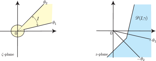
Figure 1: $1$-summability in an arc of directions. Left: $\hat{\varphi}({\zeta})\in\mathcal{N}(I,\gamma)$ is holomorphic in the union of a disc and a sector. Right: the domain $\mathscr{D}(I,\gamma)$ where $\mathcal{L}^{I}\hat{\varphi}(z)$ is holomorphic.

Observe that, for a given $z\in\mathscr{D}(I,\gamma)$, there are infinitely many possible choices for ${\theta}$, which all give the same result by virtue of Lemma 9.4; $\mathscr{D}(I,\gamma)$ is a “sectorial neighbourhood of $\infty$” centred on the ray $\arg z=-{\theta}^{*}$ with aperture $\pi+|I|$, where ${\theta}^{*}$ denotes the midpoint of $I$, in the sense that, for every ${\varepsilon}>0$, it contains a sector bisected by the half-line of direction $-{\theta}^{*}$ with opening $\pi+|I|-{\varepsilon}$ (see [CNP93]).

We extend the definition of the linear map $\mathcal{L}^{I}$ to $\mathbb{C}\,\delta\oplus\mathcal{N}(I,\gamma)$ by setting $\mathcal{L}^{I}\delta\coloneqq 1$.

Definition 9.6.

Given an open interval $I$, we say that a formal series $\tilde{\varphi}_{0}(z)\in\mathbb{C}[[z^{-1}]]$ is $1$-summable in the directions of $I$ if $\mathcal{B}\tilde{\varphi}_{0}\in\mathbb{C}\,\delta\oplus\mathcal{N}(I)$. The Borel-Laplace summation operator is defined as the composition

$$\mathscr{S}^{I}\coloneqq\mathcal{L}^{I}\circ\mathcal{B}$$ (43)

acting on all such formal series, which produces functions holomorphic in sectorial neighbourhoods of $\infty$ of the form $\mathscr{D}(I,\gamma)$, with locally bounded functions $\gamma\colon\thinspace I\to\mathbb{R}$.

There is an analogue of Corollary 7.8: the product of two formal series which are $1$-summable in the directions of $I$ is itself $1$-summable in these directions, as a consequence of Lemma 9.3 and of the stability under multiplication of fine-summable series, and the properties (35) and (36) hold for the summation operator $\mathscr{S}^{I}$ too.

As for the property of asymptotic expansion, it takes the following form: if $\tilde{\varphi}_{0}(z)$ is $1$-summable in the directions of $I$, then there exists $\gamma\colon\thinspace I\to\mathbb{R}$ locally bounded such that

$$\text{$J$ relatively compact subinterval of~{}$I$}\quad\Longrightarrow\quad\mathscr{S}^{I}\tilde{\varphi}_{0}(z)\sim_{1}\tilde{\varphi}_{0}(z)\quad\text{uniformly for $z\in\mathscr{D}(J,\gamma_{|J})$}$$

(use Theorem 7.2 and Lemma 9.3). We introduce the notation

$$\mathscr{S}^{I}\tilde{\varphi}_{0}(z)\sim_{1}\tilde{\varphi}_{0}(z)\quad\text{for $z\in\mathscr{D}(I,\gamma)$}$$ (44)

for this property, thus dropping the adverb “uniformly”. Indeed we cannot claim that $\mathscr{S}^{I}\tilde{\varphi}_{0}$ admits $\tilde{\varphi}_{0}$ as uniform $1$-Gevrey asymptotic expansion for $z\in\mathscr{D}(I,\gamma)$ (this might simply be wrong for any locally bounded function $\gamma\colon\thinspace I\to\mathbb{R}$): uniform estimates are guaranteed only when restricting to relatively compact subintervals.

The reader may check that the above definition of $1$-summability in an arc of directions $I$ coincides with the definition of $k$-summability in the directions of $I$ given in [Lod13] when $k=1$.

Remark 9.7.

Suppose that $\tilde{\varphi}_{0}(z)\in\mathcal{B}^{-1}\big{(}\mathbb{C}\,\delta\oplus\mathcal{N}(I,\gamma)\big{)}$, so that the Borel sum $\varphi_{0}(z)=\mathscr{S}^{I}\tilde{\varphi}_{0}(z)$ is holomorphic in $\mathscr{D}(I,\gamma)$ with the asymptotic property (44). Of course it may happen that $\tilde{\varphi}_{0}$ is $1$-summable in the directions of an interval which is larger than $I$, in which case there will be an analytic continuation for $\varphi_{0}$ with $1$-Gevrey asymptotic expansion in a sectorial neighbourhood of $\infty$ of aperture larger than $\pi+|I|$. But even if it is not so it may happen that $\varphi_{0}$ admits analytic continuation outside $\mathscr{D}(I,\gamma)$.

An interesting phenomenon which may occur in that case is the so-called Stokes phenomenon: the asymptotic behaviour at $\infty$ of the analytic continuation of $\varphi_{0}$ may be totally different of what it was in the directions of $\mathscr{D}(I,\gamma)$, typically one may encounter oscillatory behaviour along the limiting directions $-{\theta}^{*}\pm\frac{1}{2}\big{(}{\pi}+|I|\big{)}$ (where ${\theta}^{*}$ is the midpoint of $I$) and exponential growth beyond these directions. Examples can be found in Section 10 (Euler series: Remark 10.1 and Exercise 10.1) and § 13.1 (exponential of the Stirling series).

9.4  What if $|I|>\pi$? First observe that, if $|I|\geq 2\pi$, then $\mathcal{N}(I)$ coincides with the set of entire functions of bounded exponential type and the corresponding formal series in $z$ are precisely the convergent ones by Lemma 4.2:

$$|I|\geq 2\pi\quad\Longrightarrow\quad\mathcal{B}^{-1}\big{(}\mathbb{C}\,\delta\oplus\mathcal{N}(I)\big{)}=\mathbb{C}\{z^{-1}\}.$$

This case will be dealt with in § 9.7. We thus suppose $\pi<|I|<2\pi$.

For $\hat{\varphi}\in\mathcal{N}(I,\gamma)$, we can still define a family of holomorphic functions $\varphi_{\theta}\coloneqq\mathcal{L}^{\theta}\hat{\varphi}$ holomorphic on $\pi_{\theta}\coloneqq\Pi^{\theta}_{\gamma({\theta})}$ (${\theta}\in I$), with the property that $0<{\theta}_{2}-{\theta}_{1}<\pi\;\Longrightarrow\;\pi_{{\theta}_{1}}\cap\pi_{{\theta}_{2}}\neq\emptyset$ and $\varphi_{{\theta}_{1}}\equiv\varphi_{{\theta}_{2}}$ on $\pi_{{\theta}_{1}}\cap\pi_{{\theta}_{2}}$, but the trouble is that also for $\pi<{\theta}_{2}-{\theta}_{1}<2\pi$ is the intersection of half-planes $\pi_{{\theta}_{1}}\cap\pi_{{\theta}_{2}}$ non-empty and then nothing guarantees that $\varphi_{{\theta}_{1}}$ and $\varphi_{{\theta}_{2}}$ match on $\pi_{{\theta}_{1}}\cap\pi_{{\theta}_{2}}$.

The remedy consists in lifting the half-planes $\pi_{\theta}$ and their union $\mathscr{D}(I,\gamma)$ to the Riemann surface of the logarithm $\tilde{\mathbb{C}}=\{\,r\,{\underline{\mathrm{e}}}^{{\mathrm{i}}t}\mid r>0,\;t\in\mathbb{R}\,\}$ (see Section 24 for the definition of $\tilde{\mathbb{C}}$ and the notation ${\underline{\mathrm{e}}}^{{\mathrm{i}}t}$ which represents a point “above” the complex number $\mathrm{e}^{{\mathrm{i}}t}$). For this, we suppose $\gamma({\theta})>0$, so that $\pi_{\theta}$ is the set of all complex numbers $z=r\,\mathrm{e}^{{\mathrm{i}}t}$ with $r>\gamma({\theta})$ and $t\in\big{(}-{\theta}-\arccos\frac{\gamma({\theta})}{r},-{\theta}+\arccos\frac{\gamma({\theta})}{r}\big{)}$ (and adding any integer multiple of $2\pi$ to $t$ yields the same $z$). We set

$$\tilde{\pi}_{\theta}\coloneqq\{\,z=r\,{\underline{\mathrm{e}}}^{{\mathrm{i}}t}\in\tilde{\mathbb{C}}\mid r>\gamma({\theta}),\;t\in\big{(}-{\theta}-\arccos\tfrac{\gamma({\theta})}{r},-{\theta}+\arccos\tfrac{\gamma({\theta})}{r}\big{)}\,\},\qquad\tilde{\mathscr{D}}(I,\gamma)\coloneqq\bigcup_{{\theta}\in I}\tilde{\pi}_{\theta}$$

(this time $r\,{\underline{\mathrm{e}}}^{{\mathrm{i}}t}$ and $r\,{\underline{\mathrm{e}}}^{{\mathrm{i}}(t+2\pi m)}$ are regarded as different points of $\tilde{\mathbb{C}}$) and consider $\varphi_{\theta}=\mathcal{L}^{\theta}\hat{\varphi}$ as holomorphic in $\tilde{\pi}_{\theta}$. By gluing the various $\varphi_{\theta}$’s we now get a function which is holomorphic in $\tilde{\mathscr{D}}(I,\gamma)\subset\tilde{\mathbb{C}}$ and which we denote by $\mathcal{L}^{I}\hat{\varphi}$.

The overlap between the half-planes $\pi_{{\theta}_{1}}$ and $\pi_{{\theta}_{2}}$ for ${\theta}_{2}-{\theta}_{1}>\pi$ is no longer a problem since their lifts $\tilde{\pi}_{{\theta}_{1}}$ and $\tilde{\pi}_{{\theta}_{2}}$ do not intersect (they do not lie in the same sheet of $\tilde{\mathbb{C}}$) and $\mathcal{L}^{I}\hat{\varphi}$ may behave differently on them.

Therefore, one can extend Definition 9.6 to the case of an interval $I$ of length $>\pi$ and define $1$-summability in the directions of $I$ and the summation operator $\mathscr{S}^{I}$ the same way, except that the Borel sum $\mathscr{S}^{I}\tilde{\varphi}_{0}$ of a $1$-summable formal series $\tilde{\varphi}_{0}$ is now a function holomorphic in an open subset of the Riemann surface of the logarithm $\tilde{\mathbb{C}}$.

9.5  As already announced, the Borel sum of a convergent formal series coincides with its ordinary sum:

Lemma 9.8.

Suppose $\tilde{\varphi}_{0}\in\mathbb{C}\{z^{-1}\}$ and call $\varphi_{0}(z)$ the holomorphic function it defines for $|z|$ large enough. Then $\tilde{\varphi}_{0}$ is $1$-summable in the directions of any interval $I$ and $\mathscr{S}^{I}\tilde{\varphi}_{0}$ coincides with $\varphi_{0}$.

Proof.

Let $\tilde{\varphi}_{0}=a+\tilde{\varphi}$ with $a\in\mathbb{C}$ and $\tilde{\varphi}(z)=\sum a_{n}z^{-n-1}$, so $\varphi(z)=a+\sum a_{n}z^{-n-1}$ for $|z|$ large enough. By Lemma 4.2, $\hat{\varphi}=\mathcal{B}\tilde{\varphi}$ is a convergent formal series summing to an entire function and there exists $c>0$ such that $\hat{\varphi}\in\mathcal{N}_{c}(\mathrm{e}^{{\mathrm{i}}{\theta}}\,\mathbb{R}^{+})$ for all ${\theta}\in\mathbb{R}$. Lemma 9.4 allows us to glue together the Laplace transforms $\mathcal{L}^{\theta}\hat{\varphi}$: we get one function $\varphi_{*}$ holomorphic in $\bigcup_{{\theta}\in\mathbb{R}}\Pi^{\theta}_{c}=\{\,|z|>c\,\}$, with the asymptotic expansion property $\varphi_{*}(z)\sim_{1}\tilde{\varphi}(z)$ uniformly for $\{\,|z|>c_{1}\,\}$ for any $c_{1}>c$.

The function $\Phi_{*}\colon\thinspace t\mapsto\varphi_{*}(1/t)$ is thus holomorphic in the punctured disc $\{\,0<|t|<1/c\,\}$. Inequality (32) with $N=0$ shows that $\Phi_{*}$ is bounded, thus the origin is a removable singularity and $\Phi_{*}$ is holomorphic at $t=0$. Now inequality (32) with $N=1,2,\ldots$ shows that $\sum a_{n}t^{n+1}$ is the Taylor expansion at $0$ of $\Phi_{*}(t)$, hence $a+\varphi_{*}(1/t)\equiv\varphi_{0}(1/t)$. ∎

10 Return to the Euler series

As already mentioned (right after Definition 9.2), $\hat{\varphi}^{\raisebox{-0.69318pt}{$\scriptstyle\mathrm{E}$}}\in\mathcal{N}(I,0)$ with $I=(-\pi,\pi)$. We can thus extend the domain of analyticity of $\varphi^{\raisebox{-0.69318pt}{$\scriptstyle\mathrm{E}$}}=\mathcal{L}^{0}\hat{\varphi}^{\raisebox{-0.69318pt}{$\scriptstyle\mathrm{E}$}}$, a priori holomorphic in $\pi_{0}=\{\,\mathop{\Re e}\nolimits z>0\,\}$, by gluing the Laplace transforms $\mathcal{L}^{\theta}\hat{\varphi}^{\raisebox{-0.69318pt}{$\scriptstyle\mathrm{E}$}}$, $-\pi<{\theta}<\pi$, each of which is holomorphic in the open half-plane $\pi_{\theta}$ bisected by the ray of direction $-{\theta}$ and having the origin on its boundary. But if we take no precaution this yields a multiple-valued function: there are two possible values for $\mathop{\Re e}\nolimits z<0$, according as one uses ${\theta}$ close to $\pi$ or to $-\pi$.

A first way of presenting the situation consists in considering the subinterval $J^{+}=(0,\pi)$, the Borel sum $\varphi^{+}=\mathscr{S}^{J^{+}}\tilde{\varphi}^{\raisebox{-0.69318pt}{$\scriptstyle\mathrm{E}$}}$ holomorphic in $\mathscr{D}(J^{+},0)=\mathbb{C}\setminus{\mathrm{i}}\mathbb{R}^{+}$ which extends analytically $\varphi^{\raisebox{-0.69318pt}{$\scriptstyle\mathrm{E}$}}$ there, and $J^{-}=(-\pi,0)$, $\varphi^{-}=\mathscr{S}^{J^{-}}\tilde{\varphi}^{\raisebox{-0.69318pt}{$\scriptstyle\mathrm{E}$}}$ analytic continuation of $\varphi^{\raisebox{-0.69318pt}{$\scriptstyle\mathrm{E}$}}$ in $\mathscr{D}(J^{-},0)=\mathbb{C}\setminus{\mathrm{i}}\mathbb{R}^{-}$. See the first two parts of Figure 2.

The intersection of the domains $\mathbb{C}\setminus{\mathrm{i}}\mathbb{R}^{+}$ and $\mathbb{C}\setminus{\mathrm{i}}\mathbb{R}^{-}$ has two connected components, the half-planes $\{\,\mathop{\Re e}\nolimits z>0\,\}$ and $\{\,\mathop{\Re e}\nolimits z<0\,\}$; both functions $\varphi^{+}$ and $\varphi^{-}$ coincide with $\varphi^{\raisebox{-0.69318pt}{$\scriptstyle\mathrm{E}$}}$ on the former, whereas a simple adaptation of the proof of Lemma 9.4 involving Cauchy’s residue theorem yields

$$\mathop{\Re e}\nolimits z<0\enspace\Longrightarrow\enspace\varphi^{+}(z)-\varphi^{-}(z)=2\pi{\mathrm{i}}\,\mathrm{e}^{z}.$$ (45)

(This corresponds to the cohomological viewpoint presented in [Lod13]: $(\varphi^{+},\varphi^{-})$ defines a $0$-cochain.)

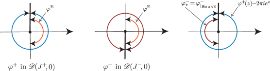
Figure 2: Borel sums of the Euler series. Left and middle: $\varphi^{\pm}$ extends $\varphi^{\raisebox{-0.62386pt}{$\scriptstyle\mathrm{E}$}}$ in the cut plane $\mathscr{D}(J^{\pm},0)$. Right: $\varphi^{+}(z)-2\pi{\mathrm{i}}\,\mathrm{e}^{z}$ extends $\varphi^{-}_{*}=\varphi^{-}_{|\{\mathop{\Re e}\nolimits z<0\}}$ in the cut plane $\mathscr{D}(J^{+},0)$.

Another way of putting it is to declare that $\varphi^{\raisebox{-0.69318pt}{$\scriptstyle\mathrm{E}$}}=\mathscr{S}^{I}\tilde{\varphi}^{\raisebox{-0.69318pt}{$\scriptstyle\mathrm{E}$}}$ is a holomorphic function on

$$\tilde{\mathscr{D}}(I,0)=\{\,z\in\tilde{\mathbb{C}}\mid-\tfrac{3\pi}{2}<\arg z<\tfrac{3\pi}{2}\,\}$$

(cf. Section 9.7) and to rewrite (45) as

$$\frac{\pi}{2}<\arg z<\frac{3\pi}{2}\enspace\Longrightarrow\enspace\varphi^{\raisebox{-0.69318pt}{$\scriptstyle\mathrm{E}$}}(z\,{\underline{\mathrm{e}}}^{-2\pi{\mathrm{i}}})-\varphi^{\raisebox{-0.69318pt}{$\scriptstyle\mathrm{E}$}}(z)=2\pi{\mathrm{i}}\,\mathrm{e}^{z}.$$ (46)

Remark 10.1.

[Stokes phenomenon for $\varphi^{\raisebox{-0.69318pt}{$\scriptstyle\mathrm{E}$}}$.] Let us consider the restriction $\varphi^{-}_{*}$ of the above function $\varphi^{-}$ to the left half-plane $\{\,\mathop{\Re e}\nolimits z<0\,\}$. Using (45) we can write it as $\varphi^{+}(z)-2\pi{\mathrm{i}}\,\mathrm{e}^{z}$, where $\varphi^{+}$ is holomorphic in an open sector bisected by ${\mathrm{i}}\mathbb{R}^{-}$, namely the cut plane $\mathscr{D}^{+}=\mathbb{C}\setminus{\mathrm{i}}\mathbb{R}^{+}$, and the other term is an entire function: this provides the analytic continuation of $\varphi^{-}_{*}$ through the cut ${\mathrm{i}}\mathbb{R}^{-}$ to the whole of $\mathscr{D}^{+}$. See the third part of Figure 2.

Observe that $\varphi^{+}\sim_{1}\tilde{\varphi}^{\raisebox{-0.69318pt}{$\scriptstyle\mathrm{E}$}}$ in $\mathscr{D}^{+}$, in particular it tends to $0$ at $\infty$ along the directions contained in $\mathscr{D}^{+}$, while the exponential $\mathrm{e}^{z}$ oscillates along ${\mathrm{i}}\mathbb{R}^{-}$ and is exponentially growing in the right half-plane: we see that, for $\varphi^{-}$, the asymptotic behaviour encoded by $\tilde{\varphi}^{\raisebox{-0.69318pt}{$\scriptstyle\mathrm{E}$}}$ in the left half-plane breaks when we cross the limiting direction ${\mathrm{i}}\mathbb{R}^{-}$; the asymptotic behaviour of the analytic continuation is oscillatory on ${\mathrm{i}}\mathbb{R}^{-}$ (up to a correction which tends to $0$) and after the crossing we find exponential growth.

A similar analysis can be performed with $\varphi^{+}_{*}=\varphi^{+}_{|\{\mathop{\Re e}\nolimits z<0\}}$ when one crosses ${\mathrm{i}}\mathbb{R}^{+}$, writing it as $\varphi^{-}(z)+2\pi{\mathrm{i}}\,\mathrm{e}^{z}$. This is a manifestation of the Stokes phenomenon evoked in Remark 9.7.

Exercise 10.1.

Use (46) to prove that $\varphi^{\raisebox{-0.69318pt}{$\scriptstyle\mathrm{E}$}}$ is the restriction to $\tilde{\mathscr{D}}(I,0)$ of a function which is holomorphic in the whole of $\tilde{\mathbb{C}}$. (Hint: Show that the formula $z\in\tilde{\mathbb{C}}\mapsto\varphi(z)\coloneqq\varphi^{\raisebox{-0.69318pt}{$\scriptstyle\mathrm{E}$}}(z\,{\underline{\mathrm{e}}}^{-2\pi{\mathrm{i}}m})-2\pi{\mathrm{i}}m\,\mathrm{e}^{z}$ if $m\in\mathbb{Z}$ and $\arg z\in(2\pi m-\frac{3\pi}{2},2\pi m+\frac{3\pi}{2})$ makes sense.) In which sectors of $\tilde{\mathbb{C}}$ is the Euler series asymptotic to this function?

Exercise 10.2.

What kind of singularity has $\varphi^{\raisebox{-0.69318pt}{$\scriptstyle\mathrm{E}$}}(z)$ when $|z|\to 0$? (Hint: Find an elementary function $L(z)$ such that $L(z\,{\underline{\mathrm{e}}}^{-2\pi{\mathrm{i}}})-L(z)=-2\pi{\mathrm{i}}\,\mathrm{e}^{z}$ and consider $\varphi^{\raisebox{-0.69318pt}{$\scriptstyle\mathrm{E}$}}+L$.)

Observe that the Euler equation $-\frac{{\mathrm{d}}\varphi}{{\mathrm{d}}z}+\varphi=z^{-1}$ is a non-homogeneous linear differential equation; the solutions of the associated homogeneous equation are the functions $\lambda\,\mathrm{e}^{z}$, $\lambda\in\mathbb{C}$. By virtue of the general properties of the summation operator $\mathscr{S}^{\theta}$, any Borel sum of $\tilde{\varphi}^{\raisebox{-0.69318pt}{$\scriptstyle\mathrm{E}$}}$ is an analytic solution of the Euler equation. In particular, the Borel sums $\varphi^{+}$ and $\varphi^{-}$ are solutions each in its own domain of definition; on formula (45) we can check that their restrictions to $\{\mathop{\Re e}\nolimits z<0\}$ differ by a solution of the homogeneous equation, as should be. In fact, any two branches of the analytic continuation of $\varphi^{\raisebox{-0.69318pt}{$\scriptstyle\mathrm{E}$}}$ differ by an integer multiple of $2\pi{\mathrm{i}}\,\mathrm{e}^{z}$. Among all the solutions of the Euler equation, $\varphi^{\raisebox{-0.69318pt}{$\scriptstyle\mathrm{E}$}}$ can be characterised as the only one which tends to $0$ when $z\to\infty$ along a ray of direction $\in(-\frac{\pi}{2},\frac{\pi}{2})$ (whereas, in the directions of $(\frac{\pi}{2},\frac{3\pi}{2})$, this is no longer a distinctive property of $\varphi^{\raisebox{-0.69318pt}{$\scriptstyle\mathrm{E}$}}$: all the solutions tend to $0$ in those directions!).

Exercise 10.3.

How can one use the so-called method of “variation of constants” to find directly an integral formula for the solution $\varphi^{\raisebox{-0.69318pt}{$\scriptstyle\mathrm{E}$}}$ of the Euler equation?

11 The Stirling series

The Stirling series is a classical example of divergent formal series, which is connected to Euler’s gamma function. The latter is the holomorphic function defined by the formula

$${\Gamma}(z)=\int_{0}^{+\infty}t^{z-1}\mathrm{e}^{-t}\,{\mathrm{d}}t$$ (47)

for any $z\in\mathbb{C}$ with $\mathop{\Re e}\nolimits z>0$ (so as to ensure the convergence of the integral). Integrating by parts, one gets the functional equation

$${\Gamma}(z+1)=z{\Gamma}(z).$$ (48)

This equation provides the analytic continuation of ${\Gamma}$ for $z\in\mathbb{C}\setminus(-\mathbb{N})$ in the form

$${\Gamma}(z)=\frac{{\Gamma}(z+n)}{z(z+1)\cdots(z+n-1)}$$ (49)

with any non-negative integer $n>-\mathop{\Re e}\nolimits z$; thus ${\Gamma}$ is meromorphic in $\mathbb{C}$ with simple poles at the non-positive integers. Since ${\Gamma}(1)=1$, the functional equation also shows that

$${\Gamma}(n+1)=n!,\qquad n\in\mathbb{N}.$$ (50)

Our starting point will be Stirling’s formula for the restriction of ${\Gamma}$ to the positive real axis:

Lemma 11.1.

$$\left(\frac{x}{2\pi}\right)^{\frac{1}{2}}x^{-x}\mathrm{e}^{x}\,{\Gamma}(x)\xrightarrow[x\to+\infty]{}1.$$ (51)

Proof.

This is an exercise in real analysis (and, as such, the following proof has nothing to do with the rest of the text!). In view of the functional equation, it is sufficient to prove that the function

$$f(x)\coloneqq\frac{{\Gamma}(x+1)}{x^{x+\frac{1}{2}}\mathrm{e}^{-x}}=\int_{0}^{+\infty}\frac{t^{x}\mathrm{e}^{-t}}{x^{x}\mathrm{e}^{-x}}\frac{{\mathrm{d}}t}{x^{1/2}}$$

tends to $\sqrt{2\pi}$ as $x\to+\infty$. The idea is that the main contribution in this integral arises for $t$ close to $x$ and that, for $t=x+s$ with $s\to 0$, $\frac{t^{x}\mathrm{e}^{-t}}{x^{x}\mathrm{e}^{-x}}\sim\exp(-\frac{s^{2}}{2x})$ and $\int_{-x}^{+\infty}\exp(-\frac{s^{2}}{2x})\,\frac{{\mathrm{d}}s}{x^{1/2}}=\int_{-\sqrt{x}}^{+\infty}\exp(-\frac{\xi^{2}}{2})\,{\mathrm{d}}\xi$, which converges to

$$\int_{-\infty}^{+\infty}\mathrm{e}^{-\xi^{2}/2}\,{\mathrm{d}}\xi=\sqrt{2\pi}$$ (52)

as $x\to+\infty$. We now provide estimates to convert this into rigorous arguments.

We shall always assume $x\geq 1$. The change of variable $t=x+\xi\sqrt{x}$ yields

$$f(x)=\int_{-\infty}^{+\infty}\mathrm{e}^{g(x,\xi)}\,{\mathrm{d}}\xi,\quad\text{with}\enspace g(x,\xi)\coloneqq\bigg{(}x\log\big{(}1+\frac{\xi}{\sqrt{x}}\big{)}-\xi\sqrt{x}\bigg{)}\mathds{1}_{\{\xi>-\sqrt{x}\}}.$$ (53)

Integrating $\frac{1}{1+{\sigma}}=1-\frac{{\sigma}}{1+{\sigma}}=1-{\sigma}+\frac{{\sigma}^{2}}{1+{\sigma}}$, we get $\log(1+\tau)=\tau-\int_{0}^{\tau}\frac{{\sigma}\,{\mathrm{d}}{\sigma}}{1+{\sigma}}=\tau-\tau^{2}/2+\int_{0}^{\tau}\frac{{\sigma}^{2}\,{\mathrm{d}}{\sigma}}{1+{\sigma}}$ for any $\tau>-1$, whence

$$g(x,\xi)=-x\int_{0}^{\xi/\sqrt{x}}\frac{{\sigma}\,{\mathrm{d}}{\sigma}}{1+{\sigma}}=-\frac{\xi^{2}}{2}+x\int_{0}^{\xi/\sqrt{x}}\frac{{\sigma}^{2}\,{\mathrm{d}}{\sigma}}{1+{\sigma}}$$ (54)

for any $\xi>-\sqrt{x}$. Since $\int_{0}^{\tau}\frac{{\sigma}^{2}\,{\mathrm{d}}{\sigma}}{1+{\sigma}}=O(\tau^{3})$ as $\tau\to 0$, the last part of (54) shows that

$$g(x,\xi)\xrightarrow[x\to+\infty]{}-\xi^{2}/2\quad\text{for each $\xi\in\mathbb{R}$}.$$

We shall use the first part of (54) to show that

1. for $-\sqrt{x}<\xi\leq 0$, $g(x,\xi)\leq-\xi^{2}/2$, whence $e^{g(x,\xi)}\leq G_{1}(\xi)\coloneqq\mathrm{e}^{-\xi^{2}/2}$;

2. for $0\leq\xi\leq\sqrt{x}$, $g(x,\xi)\leq-\xi^{2}/4$, whence $e^{g(x,\xi)}\leq G_{2}(\xi)\coloneqq\mathrm{e}^{-\xi^{2}/4}$;

3. for $\xi\geq\sqrt{x}$, $g(x,\xi)\leq-\xi/2$, whence $e^{g(x,\xi)}\leq G_{3}(\xi)\coloneqq\mathrm{e}^{-|\xi|/2}$.

This is sufficient to conclude by means of Lebesgue’s dominated convergence theorem, since this will yield $e^{g(x,\xi)}\leq G_{1}(\xi)+G_{2}(\xi)+G_{3}(\xi)$ for all $x\geq 1$ and $\xi\in\mathbb{R}$ and the function $G_{1}+G_{2}+G_{3}$ is independent of $x$ and integrable on $\mathbb{R}$, thus (53) implies $\displaystyle f(x)\xrightarrow[x\to+\infty]{}\int_{-\infty}^{+\infty}\lim_{x\to+\infty}\mathrm{e}^{g(x,\xi)}\,{\mathrm{d}}\xi$ and (52) yields the final result.

– Proof of (i): Assume $-\sqrt{x}<\xi\leq 0$. Changing ${\sigma}$ into $-{\sigma}$ and integrating the inequality $\frac{{\sigma}}{1-{\sigma}}\geq{\sigma}$ over ${\sigma}\in\big{[}0,|\xi|/\sqrt{x}\big{]}$, we get $g(x,\xi)=-x\int_{0}^{|\xi|/\sqrt{x}}\frac{{\sigma}\,{\mathrm{d}}{\sigma}}{1-{\sigma}}\leq-|\xi|^{2}/2$.

– Proof of (ii): Assume $0\leq\xi\leq\sqrt{x}$, observe that $\frac{{\sigma}}{1+{\sigma}}\geq\frac{{\sigma}}{2}$ for $0\leq{\sigma}\leq\xi/\sqrt{x}$ and integrate.

– Proof of (iii): Assume $\xi\geq\sqrt{x}\geq 1$. Noticing that $\frac{{\sigma}}{1+{\sigma}}\geq\frac{1}{2}$ for ${\sigma}\geq 1$, we get $\int_{0}^{\xi/\sqrt{x}}\frac{{\sigma}\,{\mathrm{d}}{\sigma}}{1+{\sigma}}\geq\int_{1}^{\xi/\sqrt{x}}\frac{{\sigma}\,{\mathrm{d}}{\sigma}}{1+{\sigma}}\geq\frac{\xi}{2\sqrt{x}}$, hence $g(x,\xi)\leq-\frac{1}{2}\xi\sqrt{x}\leq-\frac{\xi}{2}$.

∎

Observe that the left-hand side of (51) extends to a holomorphic function in a cut plane:

$$\lambda(z)\coloneqq\frac{1}{\sqrt{2\pi}}z^{\frac{1}{2}-z}\mathrm{e}^{z}\,{\Gamma}(z),\qquad z\in\mathbb{C}\setminus\mathbb{R}^{-}$$ (55)

(using the principal branch of the logarithm (116) to define $z^{\frac{1}{2}-z}\coloneqq\mathrm{e}^{(\frac{1}{2}-z)\mathrm{Log\hskip 1.5pt}z}$; in fact, $\lambda$ has a meromorphic continuation to the Riemann surface of the logarithm $\tilde{\mathbb{C}}$ defined in Section 24).

Theorem 11.2.

Let $I=(-\frac{\pi}{2},\frac{\pi}{2})$. The above function $\lambda$ can be written $\mathrm{e}^{\mathscr{S}^{I}\tilde{\mu}}$, where $\tilde{\mu}(z)\in z^{-1}\mathbb{C}[[z^{-1}]]$ is a divergent odd formal series which is $1$-summable in the directions of $I$, whose formal Borel transform belongs to $\mathcal{N}(I,0)$ and is explicitly given by

$$\hat{\mu}({\zeta})={\zeta}^{-2}\left(\frac{{\zeta}}{2}\coth\frac{{\zeta}}{2}-1\right),\qquad{\zeta}\in\mathbb{C}\setminus(\Delta^{+}\cup\Delta^{-})$$ (56)

where $\Delta^{\pm}$ is the half-line $\pm 2\pi{\mathrm{i}}[1,+\infty)$, and whose Borel sum $\mathscr{S}^{I}\tilde{\mu}$ is holomorphic in the cut plane $\mathscr{D}(I,0)=\mathbb{C}\setminus\mathbb{R}^{-}$.

It is the formal series $\tilde{\mu}(z)$, the asymptotic expansion of $\log\lambda(z)$, that is usually called the Stirling series.

Exercise 11.1.

Compute the Taylor expansion of the right-hand side of (56) in terms of the Bernoulli numbers $B_{2k}$ defined by $\displaystyle\frac{{\zeta}}{\mathrm{e}^{\zeta}-1}=1-\frac{1}{2}{\zeta}+\sum_{k\geq 1}\frac{B_{2k}}{(2k)!}{\zeta}^{2k}$ (so $B_{2}=1/6$, $B_{4}=-1/30$, $B_{6}=1/42$, etc.). Deduce that

$$\tilde{\mu}(z)=\sum_{k\geq 1}\frac{B_{2k}}{2k(2k-1)}z^{-2k+1}=\frac{1}{12}z^{-1}-\frac{1}{360}z^{-3}+\frac{1}{1260}z^{-5}+\cdots.$$ (57)

We shall see in § 13.1 that one can pass from $\tilde{\mu}$ to its exponential and get an improvement of (51) in the form of

Corollary 11.3 (Refined Stirling formula).

The formal series $\tilde{\lambda}(z)\coloneqq\mathrm{e}^{\tilde{\mu}(z)}$ is $1$-summable in the directions of $(-\frac{\pi}{2},\frac{\pi}{2})$ and its Borel sum is the function $\lambda$, with

$$\lambda(z)=\tfrac{1}{\sqrt{2\pi}}z^{\frac{1}{2}-z}\mathrm{e}^{z}\,{\Gamma}(z)\sim_{1}\tilde{\lambda}(z)=1+\sum_{n\geq 0}g_{n}z^{-n-1}\enspace\text{uniformly for $|z|>c$ and $\arg z\in(-\beta,\beta)$}$$ (58)

for any $c>0$ and $\beta\in(0,{\pi})$, with rationals $g_{0},g_{1},g_{2},\ldots$ computable in terms of the Bernoulli numbers:

$$g_{0} =\tfrac{1}{2}B_{2}$$

$$g_{1} =\tfrac{1}{8}B_{2}^{2}$$

$$g_{2} =\tfrac{1}{48}B_{2}^{3}+\tfrac{1}{12}B_{4}$$

$$g_{3} =\tfrac{1}{384}B_{2}^{4}+\tfrac{1}{24}B_{2}B_{4}$$

$$g_{4} =\tfrac{1}{3840}B_{2}^{5}+\tfrac{1}{96}B_{2}^{2}B_{4}+\tfrac{1}{30}B_{6}$$

$$\hphantom{=}\vdots$$

Inserting the numerical values of the Bernoulli numbers, we get

$${\Gamma}(z)\sim_{1}\mathrm{e}^{-z}z^{z-\frac{1}{2}}\sqrt{2\pi}\Big{(}1+\tfrac{1}{12}z^{-1}+\tfrac{1}{288}z^{-2}-\tfrac{139}{51840}z^{-3}-\tfrac{571}{2488320}z^{-4}+\tfrac{163879}{209018880}z^{-5}+\cdots\Big{)}$$ (59)

uniformly in the domain specified in (58).

Proof of Theorem 11.2.

a) We first consider $\lambda(x)=\frac{1}{\sqrt{2\pi}}x^{\frac{1}{2}-x}\mathrm{e}^{x}\,{\Gamma}(x)$ for $x>0$. The functional equation (48) yields

$$\lambda(x+1)=(1+x^{-1})^{-\frac{1}{2}-x}\mathrm{e}\,\lambda(x).$$

Formula (47) shows that, for $x>0$, ${\Gamma}(x)>0$ thus also $\lambda(x)>0$ and we can define

$$\mu(x)\coloneqq\log\lambda(x),\qquad x>0.$$ (60)

This function is a particular solution of the linear difference equation

$$\mu(x+1)-\mu(x)=\psi(x),$$ (61)

where $\psi(x)\coloneqq\log\big{(}(1+x^{-1})^{-\frac{1}{2}-x}\mathrm{e}\big{)}=1-(\frac{1}{2}+x)\log(1+x^{-1})$.

b) Using the principal branch of the logarithm (116), holomorphic in $\mathbb{C}\setminus\mathbb{R}^{-}$, we see that $\psi$ is the restriction to $(0,+\infty)$ of a function which is holomorphic in $\mathbb{C}\setminus[-1,0]$:

$$\psi(z)=-\frac{1}{2}\mathrm{Log\hskip 1.5pt}(1+z^{-1})+z\big{(}z^{-1}-\mathrm{Log\hskip 1.5pt}(1+z^{-1})\big{)}.$$

We observe that $\psi$ is holomorphic at $\infty$ (i.e. $t\mapsto\psi(1/t)$ is holomorphic at the origin); moreover $\psi(z)=O(z^{-2})$ and its Taylor series at $\infty$ is

$$\tilde{\psi}(z)=\frac{1}{2}\tilde{L}(z)+z\big{(}z^{-1}+\tilde{L}(z)\big{)}\in z^{-2}\mathbb{C}\{z^{-1}\},\qquad\tilde{L}(z)\coloneqq-\sum_{n\geq 1}\frac{(-1)^{n-1}}{n}z^{-n}.$$

With a view to applying Corollary 4.6, we compute the Borel transform $\hat{\psi}=\mathcal{B}\tilde{\psi}$: using $\hat{L}({\zeta})=-\sum_{n\geq 1}(-{\zeta})^{n-1}/n!={\zeta}^{-1}(\mathrm{e}^{-{\zeta}}-1)$ and the last property in Lemma 4.5, we get

$$\hat{\psi}({\zeta})=\frac{1}{2}\hat{L}({\zeta})+\frac{{\mathrm{d}}\,}{{\mathrm{d}}{\zeta}}(1+\hat{L})=\frac{1}{2}{\zeta}^{-1}(\mathrm{e}^{-{\zeta}}-1)-{\zeta}^{-2}(\mathrm{e}^{-{\zeta}}-1)-{\zeta}^{-1}\mathrm{e}^{-{\zeta}}.$$

c) Corollary 4.6 shows that the difference equation $\tilde{\varphi}(z+1)-\tilde{\varphi}(z)=\tilde{\psi}(z)$ has a unique solution in $z^{-1}\mathbb{C}[[z^{-1}]]$, whose Borel transform is

$$-{\zeta}^{-2}+\frac{1}{2}{\zeta}^{-1}-{\zeta}^{-1}\frac{\mathrm{e}^{-{\zeta}}}{\mathrm{e}^{-{\zeta}}-1}={\zeta}^{-2}\left(-1+{\zeta}\bigg{(}\frac{1}{2}+\frac{1}{\mathrm{e}^{\zeta}-1}\bigg{)}\right)=\hat{\mu}({\zeta}),$$

where $\hat{\mu}({\zeta})$ is defined by (56). The formal series $\hat{\mu}({\zeta})$ is convergent and defines an even holomorphic function which extends analytically to $\mathbb{C}\setminus(\Delta^{+}\cup\Delta^{-})$ (in fact, it even extends meromorphically to $\mathbb{C}$, with simple poles on $2\pi{\mathrm{i}}\,\mathbb{Z}^{*}$).

d) Let us check that $\hat{\mu}\in\mathcal{N}(I,0)$ with $I=(-\frac{\pi}{2},\frac{\pi}{2})$. For ${\theta}_{0}\in(0,\frac{\pi}{2})$, we shall bound $|\hat{\mu}|$ in the sector ${\Sigma}=\{\,\xi\,\mathrm{e}^{{\mathrm{i}}{\theta}}\mid\xi\geq 0,\;{\theta}\in[-{\theta}_{0},{\theta}_{0}]\,\}$. Let ${\varepsilon}\coloneqq\min\{\pi,2\pi\cos{\theta}_{0}\}$, so that ${\Sigma}$ does not intersect the discs $D(\pm 2\pi{\mathrm{i}},{\varepsilon})$. Since ${\varepsilon}>0$, the number

$$A({\varepsilon})\coloneqq\sup\Big{\{}\Big{|}\coth\frac{{\zeta}}{2}\Big{|},\;{\zeta}\in\mathbb{C}\setminus\bigcup_{m\in\mathbb{Z}}D(2\pi{\mathrm{i}}\,m,{\varepsilon})\Big{\}}$$

is finite, because ${\zeta}\mapsto\coth\frac{{\zeta}}{2}$ is $2\pi{\mathrm{i}}$-periodic, continuous in the closed set $\{\,|\mathop{\Im m}\nolimits{\zeta}|\leq\pi\,\}\setminus D(0,{\varepsilon})$ and tends to $\pm 1$ as $\mathop{\Re e}\nolimits{\zeta}\to\pm\infty$; $A$ is in fact a decreasing function of ${\varepsilon}$. For ${\zeta}\in{\Sigma}\setminus D(0,1)$, we have $|\hat{\mu}({\zeta})|\leq\frac{1}{2}|{\zeta}|^{-1}A({\varepsilon})+|{\zeta}|^{-2}\leq A({\varepsilon})+1$. Since $\hat{\mu}$ is holomorphic in the disc $D(0,2\pi)$, the number $B\coloneqq\sup\{|\hat{\mu}({\zeta})|,\;{\zeta}\in D(0,1)\}$ is finite too, and we end up with

$$|\hat{\mu}({\zeta})|\leq\max\{A({\varepsilon})+1,B\},\qquad{\zeta}\in{\Sigma},$$

whence we can conclude $\hat{\mu}\in\mathcal{N}(I,0,\alpha)$ with $\alpha({\theta})=\max\big{\{}A\big{(}{\varepsilon}({\theta})\big{)}+1,B\big{\}}$, ${\varepsilon}({\theta})=\min\{\pi,2\pi|\cos{\theta}|\}$.

e) On the one hand, we have a solution $x\mapsto\mu(x)$ of equation (61): $\mu(x+1)-\mu(x)=\psi(x)$; this solution is defined for $x>0$ and Stirling’s formula (51) implies that $\mu(x)$ tends to $0$ as $x\to+\infty$.

On the other hand, we have a formal solution $\tilde{\mu}(z)$ to the equation $\tilde{\mu}(z+1)-\tilde{\mu}(z)=\tilde{\psi}(z)$, which is $1$-summable, with a Borel sum $\mu^{+}(z)\coloneqq\mathscr{S}^{I}\tilde{\mu}(z)$ holomorphic in $\mathscr{D}(I,0)=\mathbb{C}\setminus\mathbb{R}^{-}$. The property (35) for the summation operator $\mathscr{S}^{I}$ implies that

$$\mu^{+}(z+1)-\mu^{+}(z)=\mathscr{S}^{I}\tilde{\psi}(z),\qquad z\in\mathbb{C}\setminus\mathbb{R}^{-}.$$

But $\tilde{\psi}$ is the convergent Taylor expansion of $\psi$ at $\infty$, $\mathscr{S}^{I}\tilde{\psi}$ is nothing but the analytic continuation of $\psi_{|(0,+\infty)}$. The restriction of $\mu^{+}$ to $(0,+\infty)$ is thus a solution to the same difference equation (61). Moreover, the $1$-Gevrey asymptotic property implies that $\mu^{+}(x)$ tends to $0$ as $x\to+\infty$.

The difference $x\mapsto\Delta(x)\coloneqq\mu^{+}(x)-\mu(x)$ thus satisfies $\Delta(x+1)-\Delta(x)=0$ and it tends to $0$ as $x\to+\infty$, hence $\Delta\equiv 0$. ∎

Remark 11.4.

Our chain of reasoning consisted in considering $\log\lambda_{|(0,+\infty)}$ and obtaining its analytic continuation to $\mathbb{C}\setminus\mathbb{R}^{-}$ in the form $\mathscr{S}^{I}\tilde{\mu}$. As a by-product, we deduce that the holomorphic function $\lambda$ does not vanish on $\mathbb{C}\setminus\mathbb{R}^{-}$ (being the exponential of a holomorphic function), hence the function ${\Gamma}$ itself does not vanish on $\mathbb{C}\setminus\mathbb{R}^{-}$, nor does its meromorphic continuation anywhere in the complex plane in view of (49).

The formal series $\tilde{\mu}(z)$ is odd because $\hat{\mu}({\zeta})$ is even and the Borel transform $\mathcal{B}$ shifts the powers by one unit. This does not imply that $\mathscr{S}^{I}\tilde{\mu}$ is odd! The direct consequence of the oddness of $\tilde{\mu}$ is rather the following: $\tilde{\mu}$ is $1$-summable in the directions of $J=(\frac{\pi}{2},\frac{3\pi}{2})$ and the Borel sums $\mu^{+}=\mathscr{S}^{I}\tilde{\mu}$ and $\mu^{-}=\mathscr{S}^{J}\tilde{\mu}$ are related by

$$\mu^{-}(z)=-\mu^{+}(-z),\qquad z\in\mathbb{C}\setminus\mathbb{R}^{+},$$

because a change of variable in the Laplace integral yields $\mathcal{L}^{\theta}\hat{\mu}(z)=-\mathcal{L}^{{\theta}+\pi}\hat{\mu}(-z)$. The function $\mu^{-}$ is in fact another solution of the difference equation (61).

Exercise 11.2.

1. With the notations of Remark 11.4, prove that

   $$\mu^{+}(z)-\mu^{-}(z)=\sum_{m\geq 1}\frac{1}{m}\mathrm{e}^{-2\pi{\mathrm{i}}\,mz},\qquad\mathop{\Im m}\nolimits z<0$$

   by means of a residue computation (taking advantage of the existence of a meromorphic continuation to $\mathbb{C}$ for $\hat{\mu}({\zeta})$, with simple poles on $2\pi{\mathrm{i}}\mathbb{Z}^{*}$, according to (56)).

2. Deduce that, when we increase $\arg z$ above $\pi$ or diminish it below $-\pi$, the function $\mu^{+}(z)$ has a multiple-valued analytic continuation with logarithmic singularities at negative integers.

3. Deduce that $\lambda(z)=\frac{1}{(1-\mathrm{e}^{-2\pi{\mathrm{i}}z})\lambda(-z)}$ for $\mathop{\Im m}\nolimits z<0$, thus the restriction $\lambda_{|\{\mathop{\Im m}\nolimits z<0\}}$ extends meromorphically to $\mathbb{C}\setminus\mathbb{R}^{+}$ with simple poles at the negative integers.

4. Compute the residue of this meromorphic continuation at a negative integer $-k$ and check that the result is consistent with formula (55) and the fact that the residue of the simple pole of ${\Gamma}$ at $-k$ is $(-1)^{k}/k!$. (Answer: $-\frac{{\mathrm{i}}k^{k+\frac{1}{2}}\mathrm{e}^{-k}}{k!\sqrt{2\pi}}$.)

5. Repeat the previous computations with $\mathop{\Im m}\nolimits z>0$. Does one obtain the same meromorphic continuation to $\mathbb{C}\setminus\mathbb{R}^{+}$ for $\lambda_{|\{\mathop{\Im m}\nolimits z>0\}}$? (Answer: no! But why?)

6. Prove the reflection formula

   $${\Gamma}(z){\Gamma}(1-z)=\frac{\pi}{\sin(\pi z)}.$$ (62)

Exercise 11.3.

Using (48), write a functional equation for the logarithmic derivative $\psi(z)\coloneqq{\Gamma}^{\prime}(z)/{\Gamma}(z)$. Is there any solution of this equation in $\mathbb{C}[[z^{-1}]]$? Using the principal branch of the logarithm (116) and taking for granted that $\chi(z)\coloneqq\psi(z)-\mathrm{Log\hskip 1.5pt}z$ tends to $0$ as $z$ tends to $+\infty$ along the real axis, show that $\chi(z)$ is the Borel sum of a $1$-summable formal series (to be computed explicitly).

12 Return to Poincaré’s example

In Section 2, we saw Poincaré’s example of a meromorphic function $\phi(t)$ of $\mathbb{C}^{*}$ giving rise to a divergent formal series $\tilde{\phi}(t)$ (formulas (3) and (5)). There, $w=\mathrm{e}^{s}$ was a parameter, with $|w|<1$, i.e. $\mathop{\Re e}\nolimits s<0$, and we had

$$\phi(t)=\sum_{k\geq 0}\frac{w^{k}}{1+kt},\qquad\tilde{\phi}(t)=\sum_{n\geq 0}a_{n}t^{n}$$

with well-defined coefficients $a_{n}=(-1)^{n}b_{n}$ depending on $s$.

To investigate the relationship between $\phi(t)$ and $\tilde{\phi}(t)$, we now set

$$\varphi^{\raisebox{-0.69318pt}{$\scriptstyle\mathrm{P}$}}(z)=z^{-1}\phi(z^{-1})=\sum_{k\geq 0}\frac{w^{k}}{z+k},\qquad\tilde{\varphi}^{\raisebox{-0.69318pt}{$\scriptstyle\mathrm{P}$}}(z)=z^{-1}\tilde{\phi}(z^{-1})=\sum_{n\geq 0}a_{n}z^{-n-1}$$ (63)

(to place ourselves at $\infty$ and get rid of the constant term) so that $\varphi^{\raisebox{-0.69318pt}{$\scriptstyle\mathrm{P}$}}$ is a meromorphic function of $\mathbb{C}$ with simple poles at non-positive integers and $\tilde{\varphi}^{\raisebox{-0.69318pt}{$\scriptstyle\mathrm{P}$}}(z)\in z^{-1}\mathbb{C}[[z^{-1}]]$. The formal Borel transform $\hat{\varphi}^{\raisebox{-0.69318pt}{$\scriptstyle\mathrm{P}$}}({\zeta})$ of $\tilde{\varphi}^{\raisebox{-0.69318pt}{$\scriptstyle\mathrm{P}$}}(z)$ was already computed under the name $F({\zeta})$ (cf. formula (6) and the paragraph which contains it):

$$\hat{\varphi}^{\raisebox{-0.69318pt}{$\scriptstyle\mathrm{P}$}}({\zeta})=\frac{1}{1-\mathrm{e}^{s-{\zeta}}}.$$ (64)

The natural questions are now: Is $\tilde{\varphi}^{\raisebox{-0.69318pt}{$\scriptstyle\mathrm{P}$}}$ $1$-summable in any arc of directions and is $\varphi^{\raisebox{-0.69318pt}{$\scriptstyle\mathrm{P}$}}$ its Borel sum? We shall see that the answers are affirmative, with the help of a difference equation:

Lemma 12.1.

The function $\varphi^{\raisebox{-0.69318pt}{$\scriptstyle\mathrm{P}$}}$ of (63) satisfies the functional equation

$$\varphi(z)-w\varphi(z+1)=z^{-1}.$$ (65)

For any $z_{0}\in\mathbb{C}\setminus\mathbb{R}^{-}$, the restriction of $\varphi^{\raisebox{-0.69318pt}{$\scriptstyle\mathrm{P}$}}$ to the half-line $z_{0}+\mathbb{R}^{+}$ is the only bounded solution of (65) on this half-line.

Proof.

We easily see that $w\varphi^{\raisebox{-0.69318pt}{$\scriptstyle\mathrm{P}$}}(z+1)=\sum\frac{w^{k+1}}{z+1+k}=\varphi^{\raisebox{-0.69318pt}{$\scriptstyle\mathrm{P}$}}(z)-z^{-1}$ for any $z\in\mathbb{C}\setminus(-\mathbb{N})$. The boundedness of $\varphi^{\raisebox{-0.69318pt}{$\scriptstyle\mathrm{P}$}}$ on the half-lines stems from the fact that, for $z\in z_{0}+\mathbb{R}^{+}$ and $k\in\mathbb{N}$, $|z+k|\geq|\mathop{\Im m}\nolimits(z+k)|=|\mathop{\Im m}\nolimits z_{0}|$ and, if $\mathop{\Im m}\nolimits z_{0}=0$, $|z+k|\geq z_{0}>0$, hence, in all cases, $\big{|}\frac{w^{k}}{z+k}\big{|}\leq A(z_{0})|w|^{k}$ with $A(z_{0})>0$ independent of $z$.

As for the uniqueness: suppose $\varphi_{1}$ and $\varphi_{2}$ are bounded functions on $z_{0}+\mathbb{R}^{+}$ which solve (65), then $\psi\coloneqq\varphi_{2}-\varphi_{1}$ is a bounded solution of the equation $\psi(z)-w\psi(z+1)=0$, which implies $\psi(z)=w^{n}\psi(z+n)$ for any $z\in z_{0}+\mathbb{R}^{+}$ and $n\in\mathbb{N}$; we get $\psi(z)=0$ by taking the limit as $n\to\infty$. ∎

But equation (65), written in the form $\varphi-wT_{1}\varphi=z^{-1}$, can also be considered in $\mathbb{C}[[z^{-1}]]$.

Lemma 12.2.

The formal series $\tilde{\varphi}^{\raisebox{-0.69318pt}{$\scriptstyle\mathrm{P}$}}$ of (63) is the unique solution of (65) in $\mathbb{C}[[z^{-1}]]$.

Proof.

It is clear that the constant term of any formal solution of (65) must vanish. We thus consider a formal series $\tilde{\varphi}(z)\in z^{-1}\mathbb{C}[[z^{-1}]]$. Let us denote its formal Borel transform by $\hat{\varphi}({\zeta})\in\mathbb{C}[[{\zeta}]]$; in view of the second property of Lemma 4.5, $\tilde{\varphi}$ is solution of (65) if and only if $(1-w\,\mathrm{e}^{-{\zeta}})\hat{\varphi}({\zeta})=1$. There is a unique solution because $1-w\,\mathrm{e}^{-{\zeta}}$ is invertible in $\mathbb{C}[[{\zeta}]]$ (recall that $w\neq 1$ by assumption) and its Borel transform is $(1-w\,\mathrm{e}^{-{\zeta}})^{-1}$, which according to (64) coincides with $\hat{\varphi}^{P}({\zeta})$ (recall that $w=\mathrm{e}^{s}$). ∎

Theorem 12.3.

The formal series $\tilde{\varphi}^{\raisebox{-0.69318pt}{$\scriptstyle\mathrm{P}$}}$ is $1$-summable in the directions of $I=(-\frac{\pi}{2},\frac{\pi}{2})$ and fine-summable in the directions $\pm\frac{\pi}{2}$, with $\hat{\varphi}^{\raisebox{-0.69318pt}{$\scriptstyle\mathrm{P}$}}\in\mathcal{N}(I,0)\cap\mathcal{N}_{0}({\mathrm{i}}\mathbb{R}^{+})\cap\mathcal{N}_{0}(-{\mathrm{i}}\mathbb{R}^{-})$. Its Borel sum $\mathscr{S}^{I}\tilde{\varphi}^{P}$ coincides with the function $\varphi^{\raisebox{-0.69318pt}{$\scriptstyle\mathrm{P}$}}$ in $\mathscr{D}(I,0)=\mathbb{C}\setminus\mathbb{R}^{-}$.

Let $\omega_{k}=s-2\pi{\mathrm{i}}k$ for $k\in\mathbb{Z}$. Then, for each $k\in\mathbb{Z}$, the formal series $\tilde{\varphi}^{\raisebox{-0.69318pt}{$\scriptstyle\mathrm{P}$}}$ is $1$-summable in the directions of $J_{k}=(\arg\omega_{k},\arg\omega_{k+1})\subset(\frac{\pi}{2},\frac{3\pi}{2})$, with $\hat{\varphi}^{\raisebox{-0.69318pt}{$\scriptstyle\mathrm{P}$}}\in\mathcal{N}(J_{k},\gamma)$, $\gamma({\theta})\coloneqq\cos{\theta}$, thus $\mathscr{D}(J_{k},\gamma)$ is a sectorial neighbourhood of $\infty$ containing the real half-line $(-\infty,1)$ (see Figure 3). The Borel sum of $\tilde{\varphi}^{\raisebox{-0.69318pt}{$\scriptstyle\mathrm{P}$}}$ in the directions of $J_{k}$ is a solution of equation (65) which differs from $\varphi^{\raisebox{-0.69318pt}{$\scriptstyle\mathrm{P}$}}$ by

$$\varphi^{\raisebox{-0.69318pt}{$\scriptstyle\mathrm{P}$}}(z)-\mathscr{S}^{J_{k}}\tilde{\varphi}^{\raisebox{-0.69318pt}{$\scriptstyle\mathrm{P}$}}(z)=2\pi{\mathrm{i}}\frac{\mathrm{e}^{-\omega_{k}z}}{1-\mathrm{e}^{-2\pi{\mathrm{i}}z}}=-2\pi{\mathrm{i}}\frac{\mathrm{e}^{-\omega_{k+1}z}}{1-\mathrm{e}^{2\pi{\mathrm{i}}z}}.$$ (66)

Remark 12.4.

As a consequence of (66), we rediscover the fact that $\varphi^{\raisebox{-0.69318pt}{$\scriptstyle\mathrm{P}$}}$ not only is holomorphic in $\mathbb{C}\setminus\mathbb{R}^{-}$ but also extends to a meromorphic function of $\mathbb{C}$, with simple poles at non-positive integers (because we can express it as the sum of $2\pi{\mathrm{i}}\frac{\mathrm{e}^{-sz}}{1-\mathrm{e}^{-2\pi{\mathrm{i}}z}}$, meromorphic on $\mathbb{C}$, and $\mathscr{S}^{J_{0}}\tilde{\varphi}^{\raisebox{-0.69318pt}{$\scriptstyle\mathrm{P}$}}$, holomorphic in a sectorial neighbourhood of $\infty$ which contains $\mathbb{R}^{-}$). Similarly, each function $\mathscr{S}^{J_{k}}\tilde{\varphi}^{\raisebox{-0.69318pt}{$\scriptstyle\mathrm{P}$}}$ is meromorphic in $\mathbb{C}$, with simple poles at the positive integers.

In the course of the proof of formula (66), it will be clear that its right-hand side is exponentially flat at $\infty$ in the appropriate directions, as one might expect since it has $1$-Gevrey asymptotic expansion reduced to $0$. This right-hand side is of the form $\psi(z)=\mathrm{e}^{-sz}\chi(z)$ with a $1$-periodic function $\chi$; it is easy to check that this is the general form of the solution of the homogeneous difference equation $\psi(z)-w\psi(z+1)=0$.

Figure 3: Borel-Laplace summation for Poincaré’s example.

The proof of Theorem 12.3 makes use of

Lemma 12.5.

Let ${\sigma}\in(0,-\mathop{\Re e}\nolimits s)$ and $\delta>0$. Then there exist $A=A({\sigma})>0$ and $B=B(\delta)>0$ such that, for any ${\zeta}\in\mathbb{C}$,

$$\mathop{\Re e}\nolimits{\zeta}\geq-{\sigma}\quad\Longrightarrow\quad|\hat{\varphi}^{\raisebox{-0.69318pt}{$\scriptstyle\mathrm{P}$}}({\zeta})|\leq A,$$ (67)

$$\operatorname{dist}({\zeta},s+2\pi{\mathrm{i}}\mathbb{Z})\geq\delta\quad\Longrightarrow\quad|\hat{\varphi}^{\raisebox{-0.69318pt}{$\scriptstyle\mathrm{P}$}}({\zeta})|\leq B\,\mathrm{e}^{\mathop{\Re e}\nolimits{\zeta}}.$$ (68)

Lemma 12.5 implies Theorem 12.3.

Inequality (67) implies that

$$\hat{\varphi}^{\raisebox{-0.69318pt}{$\scriptstyle\mathrm{P}$}}\in\mathcal{N}(I,0)\cap\mathcal{N}_{0}({\mathrm{i}}\mathbb{R}^{+})\cap\mathcal{N}_{0}(-{\mathrm{i}}\mathbb{R}^{-}),$$

whence the first summability statements follow. Lemma 12.2 and the property (35) for the summation operator $\mathscr{S}^{I}$ imply that $\mathscr{S}^{I}\tilde{\varphi}^{\raisebox{-0.69318pt}{$\scriptstyle\mathrm{P}$}}$ is a solution of (65); this solution is bounded on the half-line $[1,+\infty)$, because of the property (44) (in fact it tends to $0$ on any half-line of the form $z_{0}+\mathbb{R}^{+}$), thus it coincides with $\varphi^{\raisebox{-0.69318pt}{$\scriptstyle\mathrm{P}$}}$ by virtue of Lemma 12.1.

Since $\mathop{\Re e}\nolimits{\zeta}=\gamma(\arg{\zeta})|{\zeta}|$, inequality (68) implies that

$$\hat{\varphi}^{\raisebox{-0.69318pt}{$\scriptstyle\mathrm{P}$}}\in\mathcal{N}(J_{k},\gamma,\alpha_{k})$$

with $\alpha_{k}\colon\thinspace{\theta}\in J_{k}\mapsto B\big{(}\delta_{k}({\theta})\big{)}$, $\delta_{k}({\theta})=\min\big{\{}\operatorname{dist}(\omega_{k},\mathrm{e}^{{\mathrm{i}}{\theta}}\mathbb{R}^{+}),\operatorname{dist}(\omega_{k+1},\mathrm{e}^{{\mathrm{i}}{\theta}}\mathbb{R}^{+})\big{\}}$, whence the $1$-summability in the directions of $J_{k}$ follows. Again, the Borel sum is a solution of the difference equation (65), a priori defined and holomorphic in $\mathscr{D}(J_{k},\gamma)$, which is the union of the half-planes $\Pi^{\theta}_{\gamma({\theta})}$ for ${\theta}\in J_{k}$; one can check that each of these half-planes has the point $1$ on its boundary and that the intersection $\mathscr{D}$ of $\mathscr{D}(J_{k},\gamma)$ with $\mathbb{C}\setminus\mathbb{R}^{-}$ is connected. Thus, to conclude, it is sufficient to prove (66) for $z$ belonging to one of the open subdomains $\mathscr{D}_{1}^{+}\coloneqq\Pi^{\theta}_{\gamma({\theta})+1}\cap\Pi^{\pi/2}_{1}$ or $\mathscr{D}_{1}^{-}\coloneqq\Pi^{\theta}_{\gamma({\theta})+1}\cap\Pi^{-\pi/2}_{1}$, with an arbitrary ${\theta}\in J_{k}$ (none of them is empty).

Without loss of generality we can suppose ${\theta}\neq\pi$. If ${\theta}\in(\frac{\pi}{2},\pi)$, we proceed as follows: for any integer $\ell\leq k$, the horizontal line through the midpoint of $(\omega_{\ell},\omega_{\ell-1})$ cuts the half-lines $\mathrm{e}^{{\mathrm{i}}{\theta}}\mathbb{R}^{+}$ and ${\mathrm{i}}\mathbb{R}^{+}$ in the points $R_{\ell}\,\mathrm{e}^{{\mathrm{i}}{\theta}}$ and ${\mathrm{i}}R_{\ell}\sin{\theta}$, where $R_{\ell}$ is a positive real number which tends to $+\infty$ as $\ell\to\infty$ (see Figure 3). Thus, for $z\in\mathscr{D}_{1}^{+}$, we have

$$\varphi^{\raisebox{-0.69318pt}{$\scriptstyle\mathrm{P}$}}(z)=\mathcal{L}^{\pi/2}\hat{\varphi}^{\raisebox{-0.69318pt}{$\scriptstyle\mathrm{P}$}}(z) =\lim_{\ell\to\infty}\int_{0}^{{\mathrm{i}}R_{\ell}\sin{\theta}}\mathrm{e}^{-z{\zeta}}\hat{\varphi}^{\raisebox{-0.69318pt}{$\scriptstyle\mathrm{P}$}}({\zeta})\,{\mathrm{d}}{\zeta},$$

$$\mathscr{S}^{J_{k}}\tilde{\varphi}^{\raisebox{-0.69318pt}{$\scriptstyle\mathrm{P}$}}(z)=\mathcal{L}^{{\theta}}\hat{\varphi}^{\raisebox{-0.69318pt}{$\scriptstyle\mathrm{P}$}}(z) =\lim_{\ell\to\infty}\int_{0}^{R_{\ell}\,\mathrm{e}^{{\mathrm{i}}{\theta}}}\mathrm{e}^{-z{\zeta}}\hat{\varphi}^{\raisebox{-0.69318pt}{$\scriptstyle\mathrm{P}$}}({\zeta})\,{\mathrm{d}}{\zeta}.$$

Formula (64) shows that $\hat{\varphi}^{\raisebox{-0.69318pt}{$\scriptstyle\mathrm{P}$}}$ is meromorphic, with simple poles at the points $\omega_{m}$, $m\in\mathbb{Z}$, and residue $=1$ at each of these poles. Cauchy’s Residue Theorem implies that, for each $\ell\leq k$,

$$\left(\int_{0}^{{\mathrm{i}}R_{\ell}\sin{\theta}}-\int_{0}^{R_{\ell}\,\mathrm{e}^{{\mathrm{i}}{\theta}}}\right)\mathrm{e}^{-z{\zeta}}\hat{\varphi}^{\raisebox{-0.69318pt}{$\scriptstyle\mathrm{P}$}}({\zeta})\,{\mathrm{d}}{\zeta}=2\pi{\mathrm{i}}\sum_{m=\ell}^{k}\mathrm{e}^{-\omega_{m}z}+\int_{L_{\ell}}\mathrm{e}^{-z{\zeta}}\hat{\varphi}^{\raisebox{-0.69318pt}{$\scriptstyle\mathrm{P}$}}({\zeta})\,{\mathrm{d}}{\zeta},$$ (69)

where $L_{\ell}$ is the line segment $[R_{\ell}\,\mathrm{e}^{{\mathrm{i}}{\theta}},{\mathrm{i}}R_{\ell}\sin{\theta}]$. As in the proof of Lemma 9.4, we have

$$\arg{\zeta}\in\left[\tfrac{\pi}{2},{\theta}\right]\quad\Longrightarrow\quad|\mathrm{e}^{-z{\zeta}}|\leq\mathrm{e}^{-|{\zeta}|(\gamma({\theta})+1)}=\mathrm{e}^{-\mathop{\Re e}\nolimits{\zeta}-|{\zeta}|}$$

(we have used $1\geq\gamma({\theta})+1$), thus ${\zeta}\in L_{\ell}\,\Longrightarrow\,|\mathrm{e}^{-z{\zeta}}\hat{\varphi}^{\raisebox{-0.69318pt}{$\scriptstyle\mathrm{P}$}}({\zeta})|\leq B(\pi)\,\mathrm{e}^{-|{\zeta}|}\leq B(\pi)\,\mathrm{e}^{-R_{\ell}\sin{\theta}}$. Hence the integral in the right-hand side of (69) tends to $0$ and we are left with the geometric series $\mathrm{e}^{-\omega_{k}z}+\mathrm{e}^{-\omega_{k-1}z}+\cdots=\mathrm{e}^{-\omega_{k}z}\sum_{n\geq 0}\mathrm{e}^{-2\pi{\mathrm{i}}nz}$ (since $-\omega_{m}z=-\omega_{k}z-2\pi{\mathrm{i}}(k-m)z$), which yields (66).

If ${\theta}\in(\pi,\frac{3\pi}{2})$, we rather take $\ell\geq k+1$ and $z\in\mathscr{D}_{1}^{-}$ and end up with

$$\varphi^{\raisebox{-0.69318pt}{$\scriptstyle\mathrm{P}$}}(z)-\mathscr{S}^{J_{k}}\tilde{\varphi}^{\raisebox{-0.69318pt}{$\scriptstyle\mathrm{P}$}}(z)=\left(\int_{0}^{-{\mathrm{i}}\infty}-\int_{0}^{\mathrm{e}^{{\mathrm{i}}{\theta}}\infty}\right)\mathrm{e}^{-z{\zeta}}\hat{\varphi}^{\raisebox{-0.69318pt}{$\scriptstyle\mathrm{P}$}}({\zeta})\,{\mathrm{d}}{\zeta}=\\ -2\pi{\mathrm{i}}\sum_{m=k+1}^{\infty}\mathrm{e}^{-\omega_{m}z}=-2\pi{\mathrm{i}}\mathrm{e}^{-\omega_{k}z}\sum_{n\geq 1}\mathrm{e}^{2\pi{\mathrm{i}}nz},$$

which yields the same formula. ∎

Proof of Lemma 12.5.

In view of (64), for $\mathop{\Re e}\nolimits{\zeta}\geq-{\sigma}$ we have $|\mathrm{e}^{s-{\zeta}}|\leq\mathrm{e}^{{\sigma}+\mathop{\Re e}\nolimits s}<1$ and inequality (67) thus holds with $A=(1-\mathrm{e}^{{\sigma}+\mathop{\Re e}\nolimits s})^{-1}$.

Formula (64) can be rewritten as $\hat{\varphi}^{\raisebox{-0.69318pt}{$\scriptstyle\mathrm{P}$}}({\zeta})=\frac{\mathrm{e}^{\zeta}}{\mathrm{e}^{\zeta}-\mathrm{e}^{s}}$. Let $C_{\delta}\coloneqq\{\,{\zeta}\in\mathbb{C}\mid\operatorname{dist}({\zeta},s+2\pi{\mathrm{i}}\mathbb{Z})\geq\delta\,\}$ and $F({\zeta})\coloneqq|\mathrm{e}^{\zeta}-\mathrm{e}^{s}|$. The function $F$ is $2\pi{\mathrm{i}}$-periodic and does not vanish on $C_{\delta}$; since $F({\zeta})$ tends to $+\infty$ as $\mathop{\Re e}\nolimits{\zeta}\to+\infty$ and to $|w|$ as $\mathop{\Re e}\nolimits{\zeta}\to-\infty$, we can find $R>0$ such that $F({\zeta})\geq|w|/2$ for $|\mathop{\Re e}\nolimits{\zeta}|\geq R$, while $M\coloneqq\min\{\,F({\zeta})\mid{\zeta}\in C_{\delta},\,|\mathop{\Re e}\nolimits{\zeta}|\leq R,\,|\mathop{\Im m}\nolimits{\zeta}|\leq\pi\,\}$ is a well-defined positive number by compactness; (68) follows with $B=\max\{2/|w|,1/M\}$. ∎

13 Non-linear operations with $1$-summable formal series

13.1  The stability under multiplication of the space of $1$-summable formal series associated with an interval $I$ was already mentioned (right after Definition 9.6), but it is often useful to have more quantitative information on what happens in the variable ${\zeta}$, which amounts to controlling better the convolution products.

Lemma 13.1.

Suppose that ${\theta}\in\mathbb{R}$ and we are given locally integrable functions $\hat{\varphi}_{1},\hat{\varphi}_{2}\colon\thinspace\mathrm{e}^{{\mathrm{i}}{\theta}}\,\mathbb{R}^{+}\to\mathbb{C}$ and $\Phi_{1},\Phi_{2}\colon\thinspace\mathrm{e}^{{\mathrm{i}}{\theta}}\,\mathbb{R}^{+}\to\mathbb{R}^{+}$ such that

$$|\hat{\varphi}_{j}({\zeta})|\leq\Phi_{j}\big{(}|{\zeta}|\big{)},\qquad{\zeta}\in\mathrm{e}^{{\mathrm{i}}{\theta}}\,\mathbb{R}^{+}$$

for $j=1,2$ and $\Phi_{1}$, $\Phi_{2}$ are integrable on $[0,1]$. Then the convolution products $\hat{\varphi}_{3}=\hat{\varphi}_{1}*\hat{\varphi}_{2}$ and $\Phi_{3}=\Phi_{1}*\Phi_{2}$ defined by formula (24) satisfy

$$|\hat{\varphi}_{3}({\zeta})|\leq\Phi_{3}\big{(}|{\zeta}|\big{)},\qquad{\zeta}\in\mathrm{e}^{{\mathrm{i}}{\theta}}\,\mathbb{R}^{+}.$$

Proof.

Write $\hat{\varphi}_{3}({\zeta})$ as $\int_{0}^{1}\hat{\varphi}_{1}(s{\zeta})\hat{\varphi}_{2}\big{(}(1-s){\zeta}\big{)}{\zeta}\,{\mathrm{d}}s$ and $\Phi_{3}(\xi)$ as $\int_{0}^{1}\Phi_{1}(s\xi)\Phi_{2}\big{(}(1-s)\xi\big{)}\xi\,{\mathrm{d}}s$. ∎

Lemma 13.2.

Suppose $\Delta$ is an open subset of $\mathbb{C}$ which is star-shaped with respect to $0$ (i.e. it is non-empty and, for every ${\zeta}\in\Delta$, the line segment $[0,{\zeta}]$ is included in $\Delta$). Suppose $\hat{\varphi}_{1}$ and $\hat{\varphi}_{2}$ are holomorphic in $\Delta$. Then their convolution product (which is well defined since $0\in\Delta$) is also holomorphic in $\Delta$.

Proof.

The function $(s,{\zeta})\mapsto\hat{\varphi}_{1}(s{\zeta})\hat{\varphi}_{2}\big{(}(1-s){\zeta}\big{)}$ is continuous in $s$, holomorphic in ${\zeta}$ and bounded in $[0,1]\times K$ for any compact subset $K$ of $\Delta$. ∎

13.2  As an application, we show that $1$-summability is compatible with the composition operator associated with a $1$-summable formal series and with substitution into a convergent power expansion:

Theorem 13.3.

Suppose $I$ is an open interval of $\mathbb{R}$, $\tilde{\varphi}_{0}(z)=a+\tilde{\varphi}(z)$ and $\tilde{\psi}_{0}(z)$ are $1$-summable formal series in the directions of $I$, with $a\in\mathbb{C}$ and $\tilde{\varphi}(z)\in z^{-1}\mathbb{C}[[z^{-1}]]$, and $H(t)\in\mathbb{C}\{t\}$. Then the formal series $\tilde{\psi}_{0}\circ(\operatorname{id}+\tilde{\varphi}_{0})$ and $H\circ\tilde{\varphi}$ are $1$-summable in the directions of $I$ and

$$\mathscr{S}^{I}\big{(}\tilde{\psi}_{0}\circ(\operatorname{id}+\tilde{\varphi}_{0})\big{)}=(\mathscr{S}^{I}\tilde{\psi}_{0})\circ(\operatorname{id}+\mathscr{S}^{I}\tilde{\varphi}_{0}),\qquad\mathscr{S}^{I}(H\circ\tilde{\varphi})=H\circ\mathscr{S}^{I}\tilde{\varphi}.$$ (70)

More precisely, if $\mathcal{B}\tilde{\varphi}\in\mathcal{N}(I,\gamma,\alpha)$ and $\mathcal{B}\tilde{\psi}_{0}\in\mathbb{C}\,\delta\oplus\mathcal{N}(I,\gamma)$ with $\alpha,\gamma\colon\thinspace I\to\mathbb{R}$ locally bounded, $\alpha\geq 0$, and $\rho$ is a positive number smaller than the radius of convergence of $H$, then

$$\mathcal{B}\big{(}\tilde{\psi}_{0}\circ(\operatorname{id}+\tilde{\varphi}_{0})\big{)} \in\mathbb{C}\,\delta\oplus\mathcal{N}(I,\gamma_{1}), \gamma_{1} \coloneqq\gamma+|a|+\sqrt{\alpha},$$ (71)

$$\mathcal{B}(H\circ\tilde{\varphi}) \in\mathbb{C}\,\delta\oplus\mathcal{N}(I,\gamma_{2}), \gamma_{2} \coloneqq\gamma+\rho^{-1}\alpha,$$ (72)

$$z\in\mathscr{D}(I,\gamma_{1})\enspace\Longrightarrow\enspace z+\mathscr{S}^{I}\tilde{\varphi}_{0}(z)\in\mathscr{D}(I,\gamma),\qquad z\in\mathscr{D}(I,\gamma_{2})\enspace\Longrightarrow\enspace|\mathscr{S}^{I}\tilde{\varphi}(z)|\leq\rho$$ (73)

and the identities in (70) hold in $\mathscr{D}(\gamma_{1},I)$ and $\mathscr{D}(\gamma_{2},I)$ respectively.

Proof.

By assumption, $\hat{\varphi}=\mathcal{B}\tilde{\varphi}\in\mathcal{N}(I,\gamma,\alpha)$. The properties (73) are easily obtained as a consequence of

$$z\in\Pi^{\theta}_{\gamma_{j}({\theta})}\quad\Longrightarrow\quad\mathscr{S}^{I}\tilde{\varphi}(z)=\mathcal{L}^{\theta}\hat{\varphi}(z)\enspace\text{and}\enspace|\mathcal{L}^{\theta}\hat{\varphi}(z)|\leq\frac{\alpha({\theta})}{\gamma_{j}({\theta})-\gamma({\theta})}$$ (74)

for any ${\theta}\in I$ and $j=1,2$.

Let $\tilde{\psi}_{0}(z)=b+\tilde{\psi}(z)$ and $H=c+h(t)$ with $b,c\in\mathbb{C}$ and $\tilde{\psi}(z)\in z^{-1}\mathbb{C}[[z^{-1}]]$, $h(t)\in t\mathbb{C}\{t\}$, so that

$$\tilde{\psi}_{0}\circ(\operatorname{id}+\tilde{\varphi}_{0}) =b+\tilde{\lambda},\qquad \tilde{\lambda} \coloneqq\tilde{\psi}\circ(\operatorname{id}+\tilde{\varphi}_{0}),$$ (75)

$$H\circ\tilde{\varphi} =c+\tilde{\mu},\qquad \tilde{\mu} \coloneqq h\circ\tilde{\varphi}.$$ (76)

We recall that $\tilde{\lambda}$ and $\tilde{\mu}$ are defined by the formally convergent series of formal series

$$\tilde{\lambda}=\sum_{k\geq 0}\frac{1}{k!}(\partial^{k}\tilde{\psi})(\tilde{\varphi}_{0})^{k},\qquad\tilde{\mu}=\sum_{k\geq 1}h_{k}\tilde{\varphi}^{k},$$ (77)

where we use the notation $h(t)=\sum_{k\geq 1}h_{k}t^{k}$.

Correspondingly, in we have formally convergent series of formal series in $\mathbb{C}[[{\zeta}]]$: for instance, the Borel transform of $\tilde{\mu}$ is

$$\hat{\mu}=\sum_{k\geq 1}h_{k}\hat{\varphi}^{*k},\quad\text{where}\enspace\hat{\varphi}^{*k}=\underbrace{\hat{\varphi}*\cdots*\hat{\varphi}}_{\text{$k$ factors}}\in{\zeta}^{k-1}\mathbb{C}[[{\zeta}]].$$ (78)

But the series in the right-hand side of (78) can be viewed as a series of holomorphic functions, since $\hat{\varphi}$ is holomorphic in the union of a disc $D(0,R)$ and of the sector ${\Sigma}=\{\,\xi\,\mathrm{e}^{{\mathrm{i}}{\theta}}\mid\xi>0,\;{\theta}\in I\,\}$: the open set $D(0,R)\cup{\Sigma}$ is star-shaped with respect to $0$, thus Lemma 13.2 applies and each $\hat{\varphi}^{*k}$ is holomorphic in $D(0,R)\cup{\Sigma}$. We shall prove the normal convergence of this series of functions in each compact subset of $D(0,R)\cup{\Sigma}$ and provide appropriate bounds.

Choosing $R>0$ smaller than the radius of convergence of $\hat{\varphi}$, we have

$$|\hat{\varphi}({\zeta})| \leq A, {\zeta} \in D(0,R),$$

$$|\hat{\varphi}({\zeta})| \leq\Phi_{\theta}(\xi)\coloneqq\alpha({\theta})\,\mathrm{e}^{\gamma({\theta})\xi}, {\zeta} \in{\Sigma},$$

with a positive number $A$, using the notations $\xi=|{\zeta}|$ and ${\theta}=\arg{\zeta}$ in the second case. The computation of $\Phi_{\theta}^{*k}(\xi)$ is easy, since $\Phi_{\theta}$ can be viewed as the restriction to $\mathbb{R}^{+}$ of the Borel transform of $\alpha({\theta})T_{-\gamma({\theta})}(z^{-1})$; Lemma 13.1 thus yields

$$|\hat{\varphi}^{*k}({\zeta})| \leq A^{k}\frac{\xi^{k-1}}{(k-1)!}, {\zeta} \in D(0,R),$$ (79)

$$|\hat{\varphi}^{*k}({\zeta})| \leq\Phi_{\theta}^{*k}(\xi)=\alpha({\theta})^{k}\frac{\xi^{k-1}}{(k-1)!}\mathrm{e}^{\gamma({\theta})\xi}, {\zeta} \in{\Sigma}.$$ (80)

These inequalities, together with the fact that there exists $B>0$ such that $|h_{k}|\leq B\rho^{-k}$ for all $k\geq 1$ (because $\rho$ is smaller than the radius of convergence of $H$), imply that the series of functions $\sum h_{k}\hat{\varphi}^{*k}$ is uniformly convergent in every compact subset of $D(0,R)\cup{\Sigma}$; the sum of this series is a holomorphic function whose Taylor coefficients at $0$ coincide with those of $\hat{\mu}$, hence $\hat{\mu}({\zeta})\in\mathbb{C}\{{\zeta}\}$ and $\hat{\mu}$ extends analytically to $D(0,R)\cup{\Sigma}$.

Inequalities (80) also show that, for ${\zeta}\in{\Sigma}$,

$$|h_{k}\hat{\varphi}^{*k}({\zeta})|\leq\alpha({\theta})B\rho^{-1}\frac{\big{(}\rho^{-1}\alpha({\theta})\xi\big{)}^{k-1}}{(k-1)!}\mathrm{e}^{\gamma({\theta})\xi},$$

hence $|\hat{\mu}({\zeta})|\leq\alpha({\theta})B\rho^{-1}\exp{\big{(}(\gamma({\theta})+\rho^{-1}\alpha({\theta}))\xi\big{)}}$, i.e. $\hat{\mu}\in\mathcal{N}(I,\gamma+\rho^{-1}\alpha)$. The dominated convergence theorem shows that, for each ${\theta}\in I$ and $z\in\Pi^{\theta}_{\gamma_{2}({\theta})}$, $\mathcal{L}^{\theta}\hat{\mu}(z)$ coincides with the convergent sum of the series $\sum h_{k}(\mathcal{L}^{\theta}\hat{\varphi}^{*k})(z)=\sum h_{k}\big{(}\mathcal{L}^{\theta}\hat{\varphi}(z)\big{)}^{k}$, which is $h\big{(}\mathcal{L}^{\theta}\hat{\varphi}(z)\big{)}$, whence $\mathscr{S}^{I}\tilde{\mu}(z)\equiv h\big{(}\mathscr{S}^{I}\tilde{\varphi}(z)\big{)}$.

We now move on to the case of $\tilde{\lambda}$. Without loss of generality we can suppose that $a=0$, i.e. that there is no translation term in $\tilde{\varphi}_{0}$, since $\tilde{\lambda}=(T_{a}\tilde{\psi})\circ(\operatorname{id}+\tilde{\varphi})$, thus it will be sufficient to apply the translationless case of (70) and (71) to $T_{a}\tilde{\psi}\in\mathcal{B}^{-1}\big{(}\mathcal{N}(I,\gamma+|a|)\big{)}$: the identity (35) for $\mathscr{S}^{I}$ will yield $\mathscr{S}^{I}\Big{(}(T_{a}\tilde{\psi})\circ(\operatorname{id}+\tilde{\varphi})\Big{)}=(\mathscr{S}^{I}T_{a}\tilde{\psi})\circ(\operatorname{id}+\mathscr{S}^{I}\tilde{\varphi})=(\mathscr{S}^{I}\tilde{\psi})\circ(\operatorname{id}+a)\circ(\operatorname{id}+\mathscr{S}^{I}\tilde{\varphi})=(\mathscr{S}^{I}\tilde{\psi})\circ(\operatorname{id}+a+\mathscr{S}^{I}\tilde{\varphi})$.

When $a=0$, in view of (77) and the first property in Lemma 4.5, the formal series $\hat{\lambda}\coloneqq\mathcal{B}\tilde{\lambda}\in\mathbb{C}[[{\zeta}]]$ is given by the formally convergent series of formal series

$$\hat{\lambda}=\sum_{k\geq 0}\hat{\chi}_{k},\qquad\hat{\chi}_{k}\coloneqq\frac{1}{k!}\big{(}(-{\zeta})^{k}\hat{\psi}\big{)}*\hat{\varphi}^{*k}.$$

We now view the right-hand side as a series of holomorphic functions. Diminishing $R$ if necessary so as to make it smaller than the radius of convergence of $\hat{\psi}$ and taking $\alpha^{\prime}\colon\thinspace I\to\mathbb{R}^{+}$ locally bounded such that $\hat{\psi}\in\mathcal{N}(I,\gamma,\alpha^{\prime})$, we can find $A^{\prime}>0$ such that

$$|\hat{\psi}({\zeta})| \leq A^{\prime}, {\zeta} \in D(0,R),$$

$$|\hat{\psi}({\zeta})| \leq\Psi_{\theta}(\xi)\coloneqq\alpha^{\prime}({\theta})\,\mathrm{e}^{\gamma({\theta})\xi}, {\zeta} \in{\Sigma}.$$

Lemma 13.1 and 13.2 show that the $\hat{\chi}_{k}$’s are holomorphic in $D(0,R)\cup{\Sigma}$ and satisfy

$$|\hat{\chi}_{k}({\zeta})| \leq A^{\prime}\frac{\xi^{k}}{k!}*A^{k}\frac{\xi^{k-1}}{(k-1)!}=A^{\prime}A^{k}\frac{\xi^{2k}}{(2k)!}, {\zeta} \in D(0,R),$$ (81)

$$|\hat{\chi}_{k}({\zeta})| \leq\Big{(}\frac{\xi^{k}}{k!}\Psi_{\theta}\Big{)}*\Phi_{\theta}^{*k}(\xi)=\alpha^{\prime}({\theta})\alpha^{k}({\theta})\frac{\xi^{2k}}{(2k)!}\mathrm{e}^{\gamma({\theta})\xi}, {\zeta} \in{\Sigma}$$ (82)

(we used (79), (80) and (26)). The series $\sum\hat{\chi}_{k}$ is thus uniformly convergent in the compact subsets of $D(0,R)\cup{\Sigma}$ and sums to a holomorphic function, whose Taylor series at $0$ is $\hat{\lambda}$. Hence we can view $\hat{\lambda}$ as a holomorphic function and the last inequalities imply that $|\hat{\lambda}({\zeta})|\leq\alpha^{\prime}({\theta})\cosh\big{(}\sqrt{\alpha({\theta})}\xi\big{)}\mathrm{e}^{\gamma({\theta})\xi}\leq\alpha^{\prime}({\theta})\mathrm{e}^{(\sqrt{\alpha({\theta})}+\gamma({\theta}))\xi}$ for ${\zeta}\in{\Sigma}$. This yields $\hat{\lambda}\in\mathcal{N}(I,\gamma+\sqrt{\alpha})$ and, since $\mathcal{L}^{\theta}\hat{\chi}_{k}=\frac{1}{k!}\big{(}\big{(}\frac{{\mathrm{d}}\,}{{\mathrm{d}}z}\big{)}^{k}\mathcal{L}^{\theta}\hat{\psi}\big{)}(\mathcal{L}^{\theta}\hat{\varphi})^{k}$ (use the first property in Lemma 6.2 and the identity (34) for $\mathcal{L}^{\theta}$), the dominated convergence theorem yields $\mathscr{S}^{I}\tilde{\lambda}=(\mathscr{S}^{I}\tilde{\psi})\circ(\operatorname{id}+\mathscr{S}^{I}\tilde{\varphi})$. ∎

Exercise 13.1.

Prove the following multivariate version of the result on substitution in a convergent series: suppose that $r\geq 1$, $H(t_{1},\ldots,t_{r})\in\mathbb{C}\{t_{1},\ldots,t_{r}\}$, $I$ is an open interval of $\mathbb{R}$ and $\tilde{\varphi}_{1}(z),\ldots,\tilde{\varphi}_{r}(z)\in z^{-1}\mathbb{C}[[z^{-1}]]$ are $1$-summable in the directions of $I$; then the formal series

$$\tilde{\chi}(z)\coloneqq H\big{(}\tilde{\varphi}_{1}(z),\ldots,\tilde{\varphi}_{r}(z)\big{)}$$

is $1$-summable in the directions of $I$ and $\mathscr{S}^{I}\tilde{\chi}=H\circ(\mathscr{S}^{I}\tilde{\varphi}_{1},\ldots,\mathscr{S}^{I}\tilde{\varphi}_{r})$.

13.3  Proof of Corollary 11.3. As a consequence of Theorem 13.3, using $H(t)=\mathrm{e}^{t}$, we obtain the $1$-summability in the directions of $I=(-\frac{\pi}{2},\frac{\pi}{2})$ of the exponential $\tilde{\lambda}$ of the Stirling series $\tilde{\mu}$, whence the refined Stirling formula (58) for $\lambda=\mathrm{e}^{\mathscr{S}^{I}\tilde{\mu}}=\mathscr{S}^{I}\tilde{\lambda}$.

Exercise 13.2.

We just obtained that

$${\Gamma}(z)\sim_{1}\mathrm{e}^{-z}z^{z-\frac{1}{2}}\sqrt{2\pi}\Big{(}1+\sum_{k\geq 0}g_{k}z^{-k-1}\Big{)}\quad\text{uniformly for $|z|>c$ and $\arg z\in(-\beta,\beta)$}$$

for any $c>0$ and $\beta\in(0,{\pi})$ (with the extended notation of footnote 4). Show that

$$\frac{1}{{\Gamma}(z)}\sim_{1}\tfrac{1}{\sqrt{2\pi}}\mathrm{e}^{z}z^{-z+\frac{1}{2}}\Big{(}1+\sum_{k\geq 0}(-1)^{k+1}g_{k}z^{-k-1}\Big{)}\quad\text{uniformly for $|z|>c$ and $\arg z\in(-\beta,\beta)$}$$

for the same values of $c$ and $\beta$.

Remark 13.4.

Since $n!=n{\Gamma}(n)$ by (50) and (48), we get

$$n! \sim\frac{n^{n}\sqrt{2\pi n}}{\mathrm{e}^{n}}\Big{(}1+\frac{1}{12n}+\frac{1}{288n^{2}}-\frac{139}{51840n^{3}}-\frac{571}{2488320n^{4}}+\frac{163879}{209018880n^{5}}+\cdots\Big{)}$$

$$\frac{1}{n!} \sim\frac{\mathrm{e}^{n}}{n^{n}\sqrt{2\pi n}}\Big{(}1-\frac{1}{12n}+\frac{1}{288n^{2}}+\frac{139}{51840n^{3}}-\frac{571}{2488320n^{4}}-\frac{163879}{209018880n^{5}}+\cdots\Big{)}$$

uniformly for $n\in\mathbb{N}^{*}$. See [DeA09] for a direct proof.

Remark 13.5.

In accordance with Remark 9.7, we observe a kind of Stokes phenomenon for the function $\lambda$: it is a priori holomorphic in the cut plane $\mathbb{C}\setminus\mathbb{R}^{-}$, or equivalently in the sector $\{\,-\pi<\arg z<\pi\,\}$ of the Riemann surface of the logarithm $\tilde{\mathbb{C}}$, but Exercise 11.2 gives the ‘reflection formula’ $\lambda(z)=\frac{1}{(1-\mathrm{e}^{-2\pi{\mathrm{i}}z})\lambda(\mathrm{e}^{{\mathrm{i}}\pi}z)}$ for $-\pi<\arg z<0$, which yields a meromorphic continuation for $\lambda$ in the larger sector $\{\,-2\pi<\arg z<\pi\,\}$ (with the points $k\,\mathrm{e}^{-{\mathrm{i}}\pi}$, $k\in\mathbb{N}^{*}$, as only poles); the asymptotic property $\lambda(z)\sim_{1}\tilde{\lambda}(z)$ is valid in the directions of $(-\pi,\pi)$ but not in those of $(-2\pi,-\pi]$: the ray $\mathrm{e}^{-{\mathrm{i}}\pi}\mathbb{R}^{+}$ is singular and the reflection formula implies that, in the directions of $(-2\pi,-\pi)$, $\lambda(z)\sim-\mathrm{e}^{2\pi{\mathrm{i}}z}$, which is exponentially small (and $\mathrm{e}^{-2\pi{\mathrm{i}}z}\lambda(z)\sim_{1}-\tilde{\lambda}(z)$ there).

In fact, iterating the reflection formula we find a meromorphic continuation to the whole of $\tilde{\mathbb{C}}$, with a ‘monodromy relation’ $\lambda(z)=-\mathrm{e}^{2\pi{\mathrm{i}}z}\lambda(z\,{\underline{\mathrm{e}}}^{2\pi{\mathrm{i}}})$ (with the notations of Section 24). Outside the singular rays, the asymptotic behaviour is given by

$$\lambda(z)=(-1)^{n}\mathrm{e}^{-2\pi{\mathrm{i}}nz}\,\lambda(z\,{\underline{\mathrm{e}}}^{-2\pi{\mathrm{i}}n})\sim_{1}(-1)^{n}\mathrm{e}^{-2\pi{\mathrm{i}}nz}\,\tilde{\lambda}(z)$$

uniformly for $|z|$ large enough and $2\pi n-\beta<\arg z<2\pi n+\beta$, with arbitrary $n\in\mathbb{Z}$ and $\beta\in(0,\pi)$. Except in the initial sector of definition ($n=0$), we thus find exponential decay and growth alternating at each crossing of a singular ray ${\underline{\mathrm{e}}}^{(2n-1){\mathrm{i}}\pi}\mathbb{R}^{+}$ or of a ray ${\underline{\mathrm{e}}}^{2n{\mathrm{i}}\pi}\mathbb{R}^{+}$ on which the behaviour is oscillatory, according to the sign of $n\mathop{\Im m}\nolimits z$ (since $|\mathrm{e}^{-2\pi{\mathrm{i}}nz}|=\mathrm{e}^{2\pi n\mathop{\Im m}\nolimits z}$).

The last properties can also be deduced from formula (55).

13.4  We leave it to the reader to adapt the results of this section to fine-summable formal series in a direction ${\theta}$.

Formal tangent-to-identity diffeomorphisms

14 Germs of holomorphic diffeomorphisms

A holomorphic local diffeomorphism around $0$ is a holomorphic map $F\colon\thinspace U\to\mathbb{C}$, where $U$ is an open neighbourhood of $0$ in $\mathbb{C}$, such that $F(0)=0$ and $F^{\prime}(0)\neq 0$. The local inversion theorem shows that there is an open neighbourhood $V$ of $0$ contained in $U$ such that $F(V)$ is open and $F$ induces a biholomorphism from $V$ to $F(V)$. When we are not too much interested in the precise domains $U$ or $V$ but are ready to replace them by smaller neighrbouhoods of $0$, we may consider the germ of $F$ at $0$. This means that we consider the equivalence class of $F$ for the following equivalence relation: two holomorphic local diffeomorphisms are equivalent if there exists an open neighbourhood of $0$ on which their restrictions coincide.

It is easy to see that a germ of holomorphic diffeomorphism at $0$ can be identified with the Taylor series at $0$ of any of its representatives. Moreover, our equivalence relation is compatible with the composition and the inversion of holomorphic local diffeomorphisms. Consequently, the germs of holomorphic diffeomorphisms at $0$ make up a (nonabelian) group, isomorphic to

$$\{\,F(t)\in t\mathbb{C}\{t\}\mid F^{\prime}(0)\neq 0\,\}=\Big{\{}F(t)=\sum_{n\geq 1}c_{n}t^{n}\in\mathbb{C}\{t\}\mid c_{1}\neq 0\Big{\}}.$$

The coefficient $c_{1}=F^{\prime}(0)$ is called the “multiplier” of $F$. Obviously, for two germs of holomorphic diffeomorphisms $F$ and $G$, $(F\circ G)^{\prime}(0)=F^{\prime}(0)G^{\prime}(0)$. Therefore, the germs $F$ of holomorphic diffeomorphisms at $0$ such that $F^{\prime}(0)=1$ make up a subgroup; such germs are said to be “tangent-to-identity”.

Germs of holomorphic diffeomorphisms can also be considered at $\infty$: via the inversion $t\mapsto z=1/t$, a germ $F(t)$ at $0$ is conjugate to $f(z)=1/F(1/z)$. From now on, we focus on the tangent-to-identity case

$$F(t)=t-{\sigma}t^{2}-\tau t^{3}+\cdots=t(1-{\sigma}t-\tau t^{2}+\cdots)\in\mathbb{C}\{t\}\qquad({\sigma},\tau\in\mathbb{C}).$$ (83)

This amounts to considering germs of holomorphic diffeomorphisms at $\infty$ of the form

$$f(z)=z(1-{\sigma}z^{-1}-\tau z^{-2}+\cdots)^{-1}=z+{\sigma}+(\tau+{\sigma}^{2})z^{-1}+\cdots\in\operatorname{id}+\mathbb{C}\{z^{-1}\}.$$ (84)

For such a germ $f$, there exists $c>0$ large enough and a representative which is an injective holomorphic function in $\{\,|z|>c\,\}$. We use the notations

$$\mathscr{G}\coloneqq\operatorname{id}+\mathbb{C}\{z^{-1}\}$$

for the group of tangent-to-identity germs of holomorphic diffeomorphisms at $\infty$, and

$$\mathscr{G}_{\sigma}\coloneqq\operatorname{id}+{\sigma}+z^{-1}\mathbb{C}\{z^{-1}\}$$

when we want to keep track of the coefficient ${\sigma}$ in (84). Notice that, if $f_{1}\in\mathscr{G}_{{\sigma}_{1}}$ and $f_{2}\in\mathscr{G}_{{\sigma}_{2}}$, then $f_{1}\circ f_{2}\in\mathscr{G}_{{\sigma}_{1}+{\sigma}_{2}}$.

15 Formal diffeomorphisms

Even if we are interested in properties of the group $\mathscr{G}$, or even of a single element of $\mathscr{G}$, it is useful (as we shall see in Sections 32–37) to drop the convergence requirement and consider the larger set

$$\tilde{\mathscr{G}}=\operatorname{id}+\mathbb{C}[[z^{-1}]].$$

This is the set of formal tangent-to-identity diffeomorphisms at $\infty$, which we view as a complete metric space by means of the distance

$$d\big{(}\tilde{f},\tilde{h}\big{)}\coloneqq 2^{-\operatorname{val}(\tilde{\chi}-\tilde{\varphi})},\qquad\tilde{f}=\operatorname{id}+\tilde{\varphi},\;\tilde{h}=\operatorname{id}+\tilde{\chi},\qquad\tilde{\varphi},\tilde{\chi}\in\mathbb{C}[[z^{-1}]],$$

as we did for $\mathbb{C}[[z^{-1}]]$ in § 3. Notice that $\mathscr{G}$ appears as a dense subset of $\tilde{\mathscr{G}}$. We also use the notation

$$\tilde{\mathscr{G}}_{\sigma}=\operatorname{id}+{\sigma}+z^{-1}\mathbb{C}[[z^{-1}]]=\big{\{}\,\tilde{f}(z)=z+{\sigma}+\tilde{\varphi}(z)\mid\tilde{\varphi}\in z^{-1}\mathbb{C}[[z^{-1}]]\,\big{\}}\subset\tilde{\mathscr{G}}$$

for any ${\sigma}\in\mathbb{C}$. Via the inversion $z\mapsto 1/z$, the elements of $\tilde{\mathscr{G}}$ are conjugate to formal tangent-to-identity diffeomorphisms at $0$, i.e. formal series of the form (83) but without the convergence condition (the corresponding $F(t)$ is in $\mathbb{C}[[t]]$ but not necessarily in $\mathbb{C}\{t\}$); the elements of $\tilde{\mathscr{G}}_{\sigma}$ are conjugate to formal series of the form $F(t)=t-{\sigma}t^{2}+\cdots\in\mathbb{C}[[t]]$, by the formal analogue of (84).

Theorem 15.1.

The set $\tilde{\mathscr{G}}$ is a nonabelian topological group for the composition law

$$\tilde{f}\circ\tilde{h}\coloneqq\operatorname{id}+\tilde{\chi}+\tilde{\varphi}\circ(\operatorname{id}+\tilde{\chi}),\qquad\tilde{f}=\operatorname{id}+\tilde{\varphi},\;\tilde{h}=\operatorname{id}+\tilde{\chi},\qquad\tilde{\varphi},\tilde{\chi}\in\mathbb{C}[[z^{-1}]],$$ (85)

with $\tilde{\varphi}\circ(\operatorname{id}+\tilde{\chi})$ defined by (14). The subset

$$\tilde{\mathscr{G}}_{0}=\operatorname{id}+z^{-1}\mathbb{C}[[z^{-1}]]$$

is a subgroup of $\tilde{\mathscr{G}}$.

Notice that the definition (85) of the composition law in $\tilde{\mathscr{G}}$ can also be written

$$\tilde{f}\circ\tilde{h}=\sum_{k\geq 0}\frac{1}{k!}\tilde{\chi}^{k}\,\partial^{k}\tilde{f},\qquad\tilde{h}=\operatorname{id}+\tilde{\chi},$$ (86)

with the convention $\partial^{0}\tilde{f}=\tilde{f}=\operatorname{id}+\tilde{\varphi}$, $\partial\tilde{f}=1+\partial\tilde{\varphi}$ and $\partial^{k}\tilde{f}=\partial^{k}\tilde{\varphi}$ for $k\geq 2$.

Proof of Theorem 15.1.

The composition (85) is a continuous map $\tilde{\mathscr{G}}\times\tilde{\mathscr{G}}\to\tilde{\mathscr{G}}$ because, for $\tilde{f},\tilde{f}^{*},\tilde{h},\tilde{h}^{*}\in\tilde{\mathscr{G}}$, formula (86) implies

$$\tilde{f}\circ\tilde{h}^{*}-\tilde{f}\circ\tilde{h}=(\tilde{h}^{*}-\tilde{h})\int_{0}^{1}\partial\tilde{f}\circ\big{(}(1-t)\tilde{h}+t\tilde{h}^{*}\big{)}\,{\mathrm{d}}t$$ (87)

(where $\partial\tilde{f}\circ\big{(}(1-t)\tilde{h}+t\tilde{h}^{*}\big{)}$ is a formal series whose coefficients depend polynomially on $t$ and integration is meant coefficient-wise); this is a formal series of valuation $\geq\operatorname{val}(\tilde{h}^{*}-\tilde{h})$, by virtue of (15), hence the difference

$$\tilde{f}^{*}\circ\tilde{h}^{*}-\tilde{f}\circ\tilde{h}=(\tilde{f}^{*}-\tilde{f})\circ\tilde{h}^{*}+\tilde{f}\circ\tilde{h}^{*}-\tilde{f}\circ\tilde{h}$$

is a formal series of valuation $\geq\min\big{\{}\operatorname{val}(\tilde{f}^{*}-\tilde{f}),\operatorname{val}(\tilde{h}^{*}-\tilde{h})\big{\}}$ (using again (15)), i.e.

$$d(\tilde{f}\circ\tilde{h},\tilde{f}^{*}\circ\tilde{h}^{*})\leq\max\big{\{}d(\tilde{f},\tilde{f}^{*}),d(\tilde{h},\tilde{h}^{*})\big{\}}.$$

The subset $\tilde{\mathscr{G}}_{0}$ is clearly stable by composition.

The composition law of $\tilde{\mathscr{G}}$, when restricted to $\mathscr{G}$, boils down to the composition of holomorphic germs which is associative ($\mathscr{G}$ is a group) and $\mathscr{G}$ is a dense subset of $\tilde{\mathscr{G}}$, thus composition is associative in $\tilde{\mathscr{G}}$ too. It is not commutative in $\tilde{\mathscr{G}}$ since it is not commutative in $\mathscr{G}$. The element $\operatorname{id}$ is clearly a unit for composition in $\tilde{\mathscr{G}}$ thus we only need to show that there is a well-defined continuous inverse map $\tilde{h}\in\tilde{\mathscr{G}}\mapsto\tilde{h}^{\circ(-1)}\in\tilde{\mathscr{G}}$ and that this map leaves $\tilde{\mathscr{G}}_{0}$ invariant.

We first show that every element $\tilde{h}\in\tilde{\mathscr{G}}$ has a unique left inverse $\mathscr{L}(\tilde{h})$. Given $\tilde{h}=\operatorname{id}+\tilde{\chi}$, the equation $\tilde{f}\circ\tilde{h}=\operatorname{id}$ is equivalent to the fixed-point equation

$$\tilde{f}=\mathscr{C}(\tilde{f}),\qquad\mathscr{C}(\tilde{f})\coloneqq\operatorname{id}-(\tilde{f}\circ\tilde{h}-\tilde{f})=\operatorname{id}-\tilde{\chi}\int_{0}^{1}\partial\tilde{f}\circ(\operatorname{id}+t\tilde{\chi})\,{\mathrm{d}}t$$ (88)

(we have used (87) to get the last expression of $\mathscr{C}$). The map $\mathscr{C}\colon\thinspace\tilde{\mathscr{G}}\to\tilde{\mathscr{G}}$ is a contraction of our complete metric space, because the difference

$$\mathscr{C}(\tilde{f}^{*})-\mathscr{C}(\tilde{f})=-\tilde{\chi}\int_{0}^{1}\partial(\tilde{f}^{*}-\tilde{f})\circ(\operatorname{id}+t\tilde{\chi})\,{\mathrm{d}}t$$ (89)

has valuation $\geq\operatorname{val}(\tilde{f}^{*}-\tilde{f})+1$ (because of (15): $\operatorname{val}\big{(}\partial(\tilde{f}^{*}-\tilde{f})\circ(\operatorname{id}+t\tilde{\chi})\big{)}=\operatorname{val}\big{(}\partial(\tilde{f}^{*}-\tilde{f})\big{)}\geq\operatorname{val}(\tilde{f}^{*}-\tilde{f})+1$ for each $t$), hence $d\big{(}\mathscr{C}(\tilde{f}),\mathscr{C}(\tilde{f}^{*})\big{)}\leq\frac{1}{2}d(\tilde{f},\tilde{f}^{*})$. The Banach fixed-point theorem implies that there is a unique solution $\tilde{f}=\mathscr{L}(\tilde{h})$, obtained as the limit of the Cauchy sequence $\mathscr{L}_{n}(\tilde{h})\coloneqq\underbrace{\mathscr{C}\circ\cdots\circ\mathscr{C}}_{\text{$n$ times}}(0)$ as $n\to\infty$.

We observe that, if $\tilde{h}\in\tilde{\mathscr{G}}_{0}$, then $\mathscr{C}(\tilde{\mathscr{G}})\subset\tilde{\mathscr{G}}_{0}$, thus $\mathscr{L}_{n}(\tilde{h})\in\tilde{\mathscr{G}}_{0}$ for each $n\geq 0$ and clearly $\mathscr{L}(\tilde{h})\in\tilde{\mathscr{G}}_{0}$ in that case.

The fact that each element has a unique left inverse implies that each element is invertible: given $\tilde{h}\in\tilde{\mathscr{G}}$, its left inverse $\tilde{f}\coloneqq\mathscr{L}(\tilde{h})$ is also a right inverse because $\tilde{h}^{*}\coloneqq\mathscr{L}(\tilde{f})$ satisfies $\tilde{h}^{*}=\tilde{h}^{*}\circ(\tilde{f}\circ\tilde{h})=(\tilde{h}^{*}\circ\tilde{f})\circ\tilde{h}=\tilde{h}$, i.e. $\tilde{h}\circ\tilde{f}=\operatorname{id}$.

Finally, we check that $\mathscr{L}$ is continuous. For $\tilde{h},\tilde{h}^{*}\in\tilde{\mathscr{G}}$, we denote by $\mathscr{C},\mathscr{C}^{*}$ the corresponding maps defined by (88). For any $\tilde{f},\tilde{f}^{*}$, the difference $\mathscr{C}^{*}(\tilde{f})-\mathscr{C}(\tilde{f})=\tilde{f}\circ\tilde{h}-\tilde{f}\circ\tilde{h}^{*}$ has valuation $\geq\operatorname{val}(\tilde{h}^{*}-\tilde{h})$ (as already deduced from (87)), while $\operatorname{val}\big{(}\mathscr{C}^{*}(\tilde{f}^{*})-\mathscr{C}^{*}(\tilde{f})\big{)}\geq\operatorname{val}(\tilde{f}^{*}-\tilde{f})+1$ (as already deduced from (89)), hence $d\big{(}\mathscr{C}(\tilde{f}),\mathscr{C}^{*}(\tilde{f}^{*})\big{)}\leq\max\big{\{}d(\tilde{h},\tilde{h}^{*}),\frac{1}{2}d(\tilde{f},\tilde{f}^{*})\big{\}}$. It follows by induction that $d\big{(}\mathscr{L}_{n}(\tilde{h}),\mathscr{L}_{n}(\tilde{h}^{*})\big{)}=d\big{(}\mathscr{C}(\mathscr{L}_{n-1}(\tilde{h})),\mathscr{C}^{*}(\mathscr{L}_{n-1}(\tilde{h}^{*}))\big{)}\leq d(\tilde{h},\tilde{h}^{*})$ for every $n\geq 1$, hence $d\big{(}\mathscr{L}(\tilde{h}),\mathscr{L}(\tilde{h}^{*})\big{)}\leq d(\tilde{h},\tilde{h}^{*})$. ∎

Notice that $\tilde{\mathscr{G}}_{0}=\{\,\tilde{f}\in\tilde{\mathscr{G}}\mid d(\operatorname{id},\tilde{f})\leq\frac{1}{2}\,\}=\{\,\tilde{f}\in\tilde{\mathscr{G}}\mid d(\operatorname{id},\tilde{f})<1\,\}$ is a closed ball as well as an open ball, thus it is both closed and open for the Krull topology of $\tilde{\mathscr{G}}$.

16 Inversion in the group $\tilde{\mathscr{G}}$

There is an explicit formula for the inverse of an element of $\tilde{\mathscr{G}}$, which is a particular case of the Lagrange reversion formula (adapted to our framework):

Theorem 16.1.

For any $\tilde{\chi}\in\mathbb{C}[[z^{-1}]]$, the inverse of $\tilde{h}=\operatorname{id}+\tilde{\chi}$ can be written as the formally convergent series of formal series

$$(\operatorname{id}+\tilde{\chi})^{\circ(-1)}=\operatorname{id}+\sum_{k\geq 1}\frac{(-1)^{k}}{k!}\partial^{k-1}(\tilde{\chi}^{k}).$$ (90)

The proof of Theorem 16.1 will make use of

Lemma 16.2.

Let $\tilde{\chi}\in\mathbb{C}[[z^{-1}]]$ and $n\geq 1$. Then, for any $\tilde{\psi}\in\mathbb{C}[[z^{-1}]]$,

$$\sum_{k=0}^{n}(-1)^{k}\binom{n}{k}\tilde{\chi}^{n-k}\,\partial^{n-1}(\tilde{\chi}^{k}\tilde{\psi})=0.$$ (91)

Proof of Lemma 16.2.

Let us call $H_{n}\tilde{\psi}$ the left-hand side of (91). We have $H_{1}\tilde{\psi}=\tilde{\chi}\,\partial^{0}\tilde{\psi}-\partial^{0}(\tilde{\chi}\tilde{\psi})=0$. It is thus sufficient to prove the recursive formula

$$H_{n+1}\tilde{\psi}=-\partial H_{n}(\tilde{\chi}\tilde{\psi})+\tilde{\chi}\,\partial H_{n}\tilde{\psi}-n(\partial\tilde{\chi})H_{n}\tilde{\psi}.$$

To this end, we use the convention $\binom{n}{-1}=\binom{n}{n+1}=0$ and compute

$$-\partial H_{n}(\tilde{\chi}\tilde{\psi}) =\sum_{k=-1}^{n}(-1)^{k+1}\binom{n}{k}\partial\big{[}\tilde{\chi}^{n-k}\,\partial^{n-1}(\tilde{\chi}^{k+1}\tilde{\psi})\big{]}$$

$$=\sum_{k=0}^{n+1}(-1)^{k}\binom{n}{k-1}\partial\big{[}\tilde{\chi}^{n+1-k}\,\partial^{n-1}(\tilde{\chi}^{k}\tilde{\psi})\big{]}$$

(shifting the summation index to get the last expression), while

$$\tilde{\chi}\,\partial H_{n}\tilde{\psi} =\sum_{k=0}^{n+1}(-1)^{k}\binom{n}{k}\tilde{\chi}\,\partial\big{[}\tilde{\chi}^{n-k}\,\partial^{n-1}(\tilde{\chi}^{k}\tilde{\psi})\big{]}.$$

The Leibniz rule yields

$$-\partial H_{n}(\tilde{\chi}\tilde{\psi})+\tilde{\chi}\,\partial H_{n}\tilde{\psi}=\sum_{k=0}^{n+1}(-1)^{k}\Big{[}\binom{n}{k-1}+\binom{n}{k}\Big{]}\tilde{\chi}^{n+1-k}\,\partial^{n}(\tilde{\chi}^{k}\tilde{\psi})\\[4.30554pt] +\sum_{k=0}^{n+1}(-1)^{k}\Big{[}(n+1-k)\binom{n}{k-1}+(n-k)\binom{n}{k}\Big{]}\tilde{\chi}^{n-k}(\partial\tilde{\chi})\partial^{n-1}(\tilde{\chi}^{k}\tilde{\psi}).$$

The expression in the former bracket is $\binom{n+1}{k}$, hence the first sum is nothing but $H_{n+1}\tilde{\psi}$; the expression in the latter bracket is $n$ times $\binom{n-1}{k}+\binom{n-1}{k-1}=\binom{n}{k}$, hence the second sum is $n(\partial\tilde{\chi})H_{n}\tilde{\psi}$. ∎

Proof of Theorem 16.1.

Let $\tilde{h}=\operatorname{id}+\tilde{\chi}\in\tilde{\mathscr{G}}$. Lemma 16.2 shows that the right-hand side of (90) defines a left inverse for $\tilde{h}$. Indeed, denoting by $\tilde{f}=\operatorname{id}+\tilde{\varphi}$ this right-hand side, we have

$$\tilde{f}\circ\tilde{h}-\operatorname{id}=\tilde{\chi}+\tilde{\varphi}\circ(\operatorname{id}+\tilde{\chi})=\tilde{\chi}+\sum_{\ell\geq 0,\,k\geq 1}\frac{(-1)^{k}}{k!\ell!}\tilde{\chi}^{\ell}\,\partial^{k+\ell-1}(\tilde{\chi}^{k})=\sum_{n\geq 1}\frac{1}{n!}\tilde{H}_{n}$$

with $\tilde{H}_{n}=\sum(-1)^{k}\binom{n}{k}\tilde{\chi}^{\ell}\,\partial^{n-1}(\tilde{\chi}^{k})$, the last sum running over all pairs of non-negative integers $(k,\ell)$ such that $k+\ell=n$ (absorbing the first $\tilde{\chi}$ in $\tilde{H}_{1}$ and taking care of $k=0$ according as $n=1$ or $n\geq 2$; formal summability legitimates our Fubini-like manipulation), then Lemma 16.2 with $\tilde{\psi}=1$ says that $\tilde{H}_{n}=0$ for every $n\geq 1$. ∎

Exercise 16.1 (Lagrange reversion formula).

Prove that, with the same convention as in (86),

$$\tilde{f}\circ\tilde{h}^{\circ(-1)}=\tilde{f}+\sum_{k\geq 1}\frac{(-1)^{k}}{k!}\partial^{k-1}(\tilde{\chi}^{k}\partial\tilde{f}),\qquad\tilde{h}=\operatorname{id}+\tilde{\chi}.$$

(Hint: Use Lemma 16.2 with $\tilde{\psi}=\partial(\tilde{f}-\operatorname{id})=-1+\partial\tilde{f}$.)

Exercise 16.2.

Let $h=\operatorname{id}+\chi\in\mathscr{G}$, i.e. with $\chi\in\mathbb{C}\{z^{-1}\}$. We can thus choose $c_{0},M>0$ such that $|\chi(z)|\leq M$ for $|z|\geq c_{0}$. Show that $h^{\circ(-1)}(z)$ is convergent for $|z|\geq c_{0}+M$. (Hint: Given $\delta>M$, use the Cauchy inequalities to bound $|\partial^{k-1}(\chi^{k})(z)|$ for $|z|>c_{0}+\delta$.)

17 The group of $1$-summable formal diffeomorphisms in an arc of directions

Among all formal tangent-to-identity diffeomorphisms, we now distinguish those which are $1$-summable in an arc of directions.

Definition 17.1.

Let $I$ be an open interval of $\mathbb{R}$. Let $\gamma,\alpha\colon\thinspace I\to\mathbb{R}$ be locally bounded functions with $\alpha\geq 0$. For any ${\sigma}\in\mathbb{C}$ we define

$$\tilde{\mathscr{G}}(I,\gamma,\alpha) \coloneqq\big{\{}\,\tilde{f}=\operatorname{id}+\tilde{\varphi}_{0}\mid\tilde{\varphi}_{0}\in\mathcal{B}^{-1}\big{(}\mathbb{C}\,\delta\oplus\mathcal{N}(I,\gamma,\alpha)\big{)}\,\big{\}}, \quad\tilde{\mathscr{G}}_{\sigma}(I,\gamma,\alpha) \coloneqq\tilde{\mathscr{G}}(I,\gamma,\alpha)\cap\tilde{\mathscr{G}}_{\sigma},$$

$$\tilde{\mathscr{G}}(I,\gamma) \coloneqq\big{\{}\,\tilde{f}=\operatorname{id}+\tilde{\varphi}_{0}\mid\tilde{\varphi}_{0}\in\mathcal{B}^{-1}\big{(}\mathbb{C}\,\delta\oplus\mathcal{N}(I,\gamma)\big{)}\,\big{\}}, \quad\tilde{\mathscr{G}}_{\sigma}(I,\gamma) \coloneqq\tilde{\mathscr{G}}(I,\gamma)\cap\tilde{\mathscr{G}}_{\sigma},$$

$$\tilde{\mathscr{G}}(I) \coloneqq\big{\{}\,\tilde{f}=\operatorname{id}+\tilde{\varphi}_{0}\mid\tilde{\varphi}_{0}\in\mathcal{B}^{-1}\big{(}\mathbb{C}\,\delta\oplus\mathcal{N}(I)\big{)}\,\big{\}}, \quad\tilde{\mathscr{G}}_{\sigma}(I) \coloneqq\tilde{\mathscr{G}}(I)\cap\tilde{\mathscr{G}}_{\sigma}.$$

We extend the definition of the Borel summation operator $\mathscr{S}^{I}$ to $\tilde{\mathscr{G}}(I)$ by setting

$$\tilde{f}=\operatorname{id}+\tilde{\varphi}_{0}\in\tilde{\mathscr{G}}(I,\gamma)\quad\Longrightarrow\quad\mathscr{S}^{I}\tilde{f}(z)=z+\mathscr{S}^{I}\tilde{\varphi}^{0}(z),\qquad z\in\mathscr{D}(I,\gamma).$$

For $|I|\geq 2\pi$, $\tilde{\mathscr{G}}(I)$ coincides with the group $\mathscr{G}$ of holomorphic tangent-to-identity diffeomorphisms and $\mathscr{S}^{I}$ is the ordinary summation operator for Taylor series at $\infty$, but

$$|I|<2\pi\quad\Longrightarrow\quad\mathscr{G}\,\subsetneqq\,\tilde{\mathscr{G}}(I)\,\subsetneqq\,\tilde{\mathscr{G}}.$$

For $\tilde{f}\in\tilde{\mathscr{G}}(I)$, the function $\mathscr{S}^{I}\tilde{f}$ is holomorphic in a sectorial neighbourhood of $\infty$ (but not in a full neighbourhood of $\infty$ if $\tilde{f}\notin\mathscr{G}$); we shall see that it defines an injective transformation in a domain of the form $\mathscr{D}(I,\gamma)$. We first study composition and inversion in $\tilde{\mathscr{G}}(I)$.

Theorem 17.2.

Let $I$ be an open interval of $\mathbb{R}$ and $\gamma,\alpha\colon\thinspace I\to\mathbb{R}$ be locally bounded functions with $\alpha\geq 0$. Let ${\sigma},\tau\in\mathbb{C}$ and $\tilde{f}\in\tilde{\mathscr{G}}_{\sigma}(I,\gamma,\alpha)$, $\tilde{g}\in\tilde{\mathscr{G}}_{\tau}(I,\gamma)$. Then $\tilde{g}\circ\tilde{f}\in\tilde{\mathscr{G}}_{{\sigma}+\tau}(I,\gamma_{1})$ with $\gamma_{1}=\gamma+|{\sigma}|+\sqrt{\alpha}$, the function $\mathscr{S}^{I}\tilde{f}$ maps $\mathscr{D}(I,\gamma_{1})$ in $\mathscr{D}(I,\gamma)$ and

$$\mathscr{S}^{I}(\tilde{g}\circ\tilde{f})=(\mathscr{S}^{I}\tilde{g})\circ(\mathscr{S}^{I}\tilde{f})\enspace\text{on $\mathscr{D}(I,\gamma_{1})$}.$$

Proof.

Apply Theorem 13.3 to $\tilde{\varphi}_{0}\coloneqq\tilde{f}-\operatorname{id}$ and $\tilde{\psi}_{0}\coloneqq\tilde{g}-\operatorname{id}$. ∎

Theorem 17.3.

Let $\tilde{f}\in\tilde{\mathscr{G}}_{\sigma}(I,\gamma,\alpha)$. Then $\tilde{h}\coloneqq\tilde{f}^{\circ(-1)}\in\tilde{\mathscr{G}}_{-{\sigma}}(I,\gamma^{*},\alpha)$ with $\gamma^{*}\coloneqq\gamma+|{\sigma}|+2\sqrt{\alpha}$ and

$$\mathscr{S}^{I}\tilde{f}\big{(}\mathscr{D}(I,\gamma_{1})\big{)} \subset\mathscr{D}(I,\gamma^{*}), \enspace(\mathscr{S}^{I}\tilde{h})\circ\mathscr{S}^{I}\tilde{f} =\operatorname{id}\enspace\text{on $\mathscr{D}(I,\gamma_{1})$,}$$ (92)

$$\mathscr{S}^{I}\tilde{h}\big{(}\mathscr{D}(I,\gamma_{2})\big{)} \subset\mathscr{D}(I,\gamma), \enspace(\mathscr{S}^{I}\tilde{f})\circ\mathscr{S}^{I}\tilde{h} =\operatorname{id}\enspace\text{on $\mathscr{D}(I,\gamma_{2})$,}$$ (93)

with $\gamma_{1}\coloneqq\gamma+2|{\sigma}|+(1+\sqrt{2})\sqrt{\alpha}$ and $\gamma_{2}\coloneqq\gamma+|{\sigma}|+(1+\sqrt{2})\sqrt{\alpha}$.

Moreover, $\mathscr{S}^{I}\tilde{f}$ is injective on $\mathscr{D}\big{(}I,\gamma+(1+\sqrt{2})\sqrt{\alpha}\big{)}$.

Proof.

We first assume $\tilde{f}\in\tilde{\mathscr{G}}_{0}(I,\gamma,\alpha)$. By (90), we have $\tilde{h}=\operatorname{id}+\tilde{\chi}$ with $\tilde{\chi}$ given by a formally convergent series in $z^{-1}\mathbb{C}[[z^{-1}]]$:

$$\tilde{\chi}=\sum_{k\geq 1}\tilde{\chi}_{k},\qquad\tilde{\chi}_{k}=\frac{(-1)^{k}}{k!}\partial^{k-1}(\tilde{\varphi}^{k}).$$

Correspondingly, $\mathcal{B}\tilde{\chi}$ is given by a formally convergent series in $\mathbb{C}[[{\zeta}]]$:

$$\hat{\chi}=\sum_{k\geq 1}\hat{\chi}_{k},\qquad\hat{\chi}_{k}=-\frac{{\zeta}^{k-1}}{k!}\hat{\varphi}^{*k}$$

(beware that the last expression involves multiplication by $-\frac{{\zeta}^{k-1}}{k!}$, not convolution!). We argue as in the proof of Theorem 13.3 and view $\hat{\chi}$ as a series of holomorphic functions in the union of a disc $D(0,R)$ and a sector ${\Sigma}$ in which $\hat{\varphi}$ itself is holomorphic; inequalities (79) and (80) yield

$$|\hat{\chi}_{k}({\zeta})| \leq A^{k}\frac{\xi^{2(k-1)}}{k!(k-1)!}, {\zeta} \in D(0,R),$$ (94)

$$|\hat{\chi}_{k}({\zeta})| \leq\alpha({\theta})^{k}\frac{\xi^{2(k-1)}}{k!(k-1)!}\mathrm{e}^{\gamma({\theta})\xi}, {\zeta} \in{\Sigma},$$ (95)

where $\xi=|{\zeta}|$ and ${\theta}=\arg{\zeta}$. The series of holomorphic functions $\sum\hat{\chi}_{k}$ is thus uniformly convergent in every compact subset of $D(0,R)\cup{\Sigma}$ and its sum is a holomorphic function whose Taylor series at $0$ is $\hat{\chi}$. Therefore $\hat{\chi}\in\mathbb{C}\{{\zeta}\}$ extends analytically to $D(0,R)\cup{\Sigma}$; moreover, since $\frac{1}{k!(k-1)!}\leq\frac{1}{k}\frac{2^{2(k-1)}}{(2(k-1))!}$, (95) yields

$$|\hat{\chi}({\zeta})|\leq\sum_{k\geq 1}\frac{\alpha({\theta})^{k}}{k}\frac{(2\xi)^{2(k-1)}}{\big{(}2(k-1)\big{)}!}\mathrm{e}^{\gamma({\theta})\xi}\leq\alpha({\theta})\,\mathrm{e}^{(\gamma({\theta})+2\sqrt{\alpha({\theta})})\xi}$$

for ${\zeta}\in{\Sigma}$. Hence $\tilde{h}\in\tilde{\mathscr{G}}_{0}(I,\gamma+2\sqrt{\alpha},\alpha)$ when ${\sigma}=0$.

In the general case, we observe that $\tilde{f}=(\operatorname{id}+{\sigma})\circ\tilde{g}$ with $\tilde{g}\coloneqq(\operatorname{id}-{\sigma})\circ\tilde{f}\in\tilde{\mathscr{G}}_{0}(I,\gamma,\alpha)$, thus $\tilde{g}^{\circ(-1)}=\operatorname{id}+\tilde{\chi}\in\tilde{\mathscr{G}}_{0}(I,\gamma+2\sqrt{\alpha},\alpha)$ and $\tilde{h}=\tilde{f}^{\circ(-1)}=\tilde{g}^{\circ(-1)}\circ(\operatorname{id}-{\sigma})=\operatorname{id}-{\sigma}+T_{-{\sigma}}\tilde{\chi}$, which implies $\tilde{h}\in\tilde{\mathscr{G}}(I,\gamma+2\sqrt{\alpha}+|{\sigma}|,\alpha)$ by the second property in Lemma 4.5.

Since $\tilde{h}\circ\tilde{f}=\tilde{f}\circ\tilde{h}=\operatorname{id}$, we can apply Theorem 17.2 and get $(\mathscr{S}^{I}\tilde{h})\circ\mathscr{S}^{I}\tilde{f}=\operatorname{id}$ and $(\mathscr{S}^{I}\tilde{f})\circ\mathscr{S}^{I}\tilde{h}=\operatorname{id}$ in appropriate domains; in fact, by analytic continuation, these identities will hold in any domain $\mathscr{D}(I,\gamma+\delta_{1})$, resp. $\mathscr{D}(I,\gamma+\delta_{2})$, such that

$$\mathscr{S}^{I}\tilde{f}\big{(}\mathscr{D}(I,\gamma+\delta_{1})\big{)}\subset\mathscr{D}(I,\gamma^{*}),\qquad\mathscr{S}^{I}\tilde{h}\big{(}\mathscr{D}(I,\gamma+\delta_{2})\big{)}\subset\mathscr{D}(I,\gamma).$$

Writing $\tilde{f}=\operatorname{id}+{\sigma}+\tilde{\varphi}$ with $\mathcal{B}\tilde{\varphi}\in\mathcal{N}(I,\gamma,\alpha)$, with the help of (74) one can easily show that $\delta_{1}=\gamma_{1}-\gamma$ and $\delta_{2}=\gamma_{2}-\gamma$ satisfy this.

For the injectivity statement, we write again $\tilde{f}=(\operatorname{id}+{\sigma})\circ\tilde{g}$ and apply the previous result to $\tilde{g}\in\mathscr{G}_{0}(I,\gamma,\alpha)$. The function $\mathscr{S}^{I}\tilde{g}$ maps $\mathscr{D}\coloneqq\mathscr{D}\big{(}I,\gamma+(1+\sqrt{2})\sqrt{\alpha}\big{)}$ in the domain $\mathscr{D}\big{(}I,\gamma+2\sqrt{\alpha}\big{)}$, on which $\mathscr{S}^{I}(\tilde{g}^{\circ(-1)})$ is well-defined, and $\mathscr{S}^{I}(\tilde{g}^{\circ(-1)})\circ\mathscr{S}^{I}\tilde{g}=\operatorname{id}$ on $\mathscr{D}$, therefore $\mathscr{S}^{I}\tilde{g}$ is injective on $\mathscr{D}$, and so is the function $\mathscr{S}^{I}\tilde{f}={\sigma}+\mathscr{S}^{I}\tilde{g}$. ∎

Corollary 17.4.

For any open interval $I$, $\tilde{\mathscr{G}}(I)$ and $\tilde{\mathscr{G}}_{0}(I)$ are subgroups of $\tilde{\mathscr{G}}$.

Exercise 17.1.

Consider the set $\operatorname{id}+\mathbb{C}[[z^{-1}]]_{1}$ of $1$-Gevrey tangent-to-identity formal diffeomorphisms, so that

$$\tilde{\mathscr{G}}(I)\;\subsetneqq\;\operatorname{id}+\mathbb{C}[[z^{-1}]]_{1}\;\subsetneqq\;\tilde{\mathscr{G}}.$$

Show that $\operatorname{id}+\mathbb{C}[[z^{-1}]]_{1}$ is a subgroup of $\tilde{\mathscr{G}}$. (Hint: View $\mathbb{C}[[z^{-1}]]_{1}$ as $\mathcal{B}^{-1}\big{(}\mathbb{C}\,\delta\oplus\mathbb{C}\{{\zeta}\}\big{)}$ and imitate the previous chain of reasoning.)

We shall see in Section 34 how $1$-summable formal diffeomorphisms occur in the study of a holomorphic germ $f\in\mathscr{G}_{1}$.

The algebra of resurgent functions

18 Resurgent functions, resurgent formal series

Among $1$-Gevrey formal series, we have distinguished the subspace of those which are $1$-summable in a given arc of directions and studied it in Sections 9–17. We shall now study another subspace of $\mathbb{C}[[z^{-1}]]_{1}$, which consists of “resurgent formal series”. As in the case of $1$-summability, we make use of the algebra isomorphism (22)

$$\mathcal{B}\colon\thinspace\mathbb{C}[[z^{-1}]]_{1}\xrightarrow{\sim}\mathbb{C}\delta\oplus\mathbb{C}\{{\zeta}\}$$

and give the definition not directly in terms of the formal series themselves, but rather in terms of their formal Borel transforms, for which, beyond convergence near the origin, we shall require a certain property of analytic continuation.

For any $R>0$ and ${\zeta}_{0}\in\mathbb{C}$ we use the notations

$$D({\zeta}_{0},R)\coloneqq\{\,{\zeta}\in\mathbb{C}\mid|{\zeta}-{\zeta}_{0}|<R\,\},$$ (96)

$$\mathbb{D}_{R}\coloneqq D(0,R),\qquad\mathbb{D}^{*}_{R}\coloneqq\mathbb{D}_{R}\setminus\{0\}.$$ (97)

Definition 18.1.

Let $\Omega$ be a non-empty closed discrete subset of $\mathbb{C}$, let $\hat{\varphi}({\zeta})\in\mathbb{C}\{{\zeta}\}$ be a holomorphic germ at the origin. We say that $\hat{\varphi}$ is an $\Omega$-continuable germ if there exists $R>0$ not larger than the radius of convergence of $\hat{\varphi}$ such that $\mathbb{D}^{*}_{R}\cap\Omega=\emptyset$ and $\hat{\varphi}$ admits analytic continuation along any path of $\mathbb{C}\setminus\Omega$ originating from any point of $\mathbb{D}^{*}_{R}$. See Figure 4. We use the notation

$$\hat{\mathscr{R}}_{\Omega}\coloneqq\{\,\text{all $\Omega$-continuable germs}\,\}\subset\mathbb{C}\{{\zeta}\}.$$

We call $\Omega$-resurgent function any element of $\mathbb{C}\,\delta\oplus\hat{\mathscr{R}}_{\Omega}$, i.e. any element of $\mathbb{C}\,\delta\oplus\mathbb{C}\{{\zeta}\}$ of the form $a\,\delta+\hat{\varphi}$ with $a=$ a complex number and $\hat{\varphi}=$ an $\Omega$-continuable germ.

We call $\Omega$-resurgent formal series any $\tilde{\varphi}_{0}(z)\in\mathbb{C}[[z^{-1}]]_{1}$ whose formal Borel transform is an $\Omega$-resurgent function, i.e. any $\tilde{\varphi}_{0}$ belonging to

$$\tilde{\mathscr{R}}_{\Omega}\coloneqq\mathcal{B}^{-1}\big{(}\mathbb{C}\,\delta\oplus\hat{\mathscr{R}}_{\Omega}\big{)}\subset\mathbb{C}[[z^{-1}]]_{1}.$$

Remark 18.2.

In the above definition, “path” means a continuous function $\gamma\colon\thinspace J\to\mathbb{C}\setminus\Omega$, where $J$ is a compact interval of $\mathbb{R}$; without loss of generality, all our paths will be assumed piecewise continuously differentiable. As is often the case with analytic continuation and Cauchy integrals, the precise parametrisation of $\gamma$ will usually not matter, in the sense that we shall get the same result from two paths $\gamma\colon\thinspace[a,b]\to\mathbb{C}\setminus\Omega$ and $\gamma^{\prime}\colon\thinspace[a^{\prime},b^{\prime}]\to\mathbb{C}\setminus\Omega$ which only differ by a change of parametrisation ($\gamma=\gamma^{\prime}\circ{\sigma}$ with ${\sigma}\colon\thinspace[a,b]\to[a^{\prime},b^{\prime}]$ piecewise continuously differentiable, increasing and mapping $a$ to $a^{\prime}$ and $b$ to $b^{\prime}$).

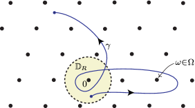
Figure 4: $\Omega$-continuability. Any path $\gamma$ starting in $\mathbb{D}_{R}^{*}$ and contained in $\mathbb{C}\setminus\Omega$ must be a path of analytic continuation for $\hat{\varphi}\in\hat{\mathscr{R}}_{\Omega}$.

Our definitions are particular cases of Écalle’s definition of “continuability without a cut” (or “endless continuability”) for germs, and “resurgence” for formal series (we prescribe in advance the possible location of the singularities of the analytic continuation of $\hat{\varphi}$, whereas the theory is developed in Vol. 3 of [Eca81] without this restriction). Here we stick to the simplest cases; typical examples with which we shall work are $\Omega=\mathbb{Z}$ or $2\pi{\mathrm{i}}\,\mathbb{Z}$.

Remark 18.3.

Let ${\rho(\Omega)}\coloneqq\min\big{\{}|\omega|,\;\omega\in\Omega\setminus\{0\}\big{\}}$. Any $\hat{\varphi}\in\hat{\mathscr{R}}_{\Omega}$ is a holomorphic germ at $0$ with radius of convergence $\geq{\rho(\Omega)}$ and one can always take $R={\rho(\Omega)}$ in Definition 18.1. In fact, given an arbitrary ${\zeta}_{0}\in\mathbb{D}_{\rho(\Omega)}$, we have

$$\hat{\varphi}\in\hat{\mathscr{R}}_{\Omega}\quad\Longleftrightarrow\quad\left|\begin{aligned} &\text{$\hat{\varphi}$ germ of holomorphic function of~{}$\mathbb{D}_{\rho(\Omega)}$ admitting analytic continuation}\\ &\text{along any path $\gamma\colon\thinspace[0,1]\to\mathbb{C}$ such that $\gamma(0)={\zeta}_{0}$ and $\gamma\big{(}(0,1]\big{)}\subset\mathbb{C}\setminus\Omega$}\end{aligned}\right.$$

(even if ${\zeta}_{0}=0$ and $0\in\Omega$: there is no need to avoid $0$ at the beginning of the path, when we still are in the disc of convergence of $\hat{\varphi}$).

Example 18.1.

Trivially, any entire function of $\mathbb{C}$ defines an $\Omega$-continuable germ; as a consequence,

$$\mathbb{C}\{z^{-1}\}\subset\tilde{\mathscr{R}}_{\Omega}.$$

Other elementary examples of $\Omega$-continuable germs are the functions which are holomorphic in $\mathbb{C}\setminus\Omega$ and regular at $0$, like $\frac{1}{({\zeta}-\omega)^{m}}$ with $m\in\mathbb{N}^{*}$ and $\omega\in\Omega\setminus\{0\}$.

Lemma 18.4.

1. The Euler series $\tilde{\varphi}^{\raisebox{-0.69318pt}{$\scriptstyle\mathrm{E}$}}(z)$ defined by (38) belongs to $\tilde{\mathscr{R}}_{\{-1\}}$.

2. Given $w=\mathrm{e}^{s}$ with $\mathop{\Re e}\nolimits s<0$, the series $\tilde{\varphi}^{\raisebox{-0.69318pt}{$\scriptstyle\mathrm{P}$}}(z)$ of Poincaré’s example (63) belongs to $\tilde{\mathscr{R}}_{\Omega}$ with $\Omega\coloneqq s+2\pi{\mathrm{i}}\,\mathbb{Z}$.

3. The Stirling series $\tilde{\mu}(z)$ of Theorem 11.2 (explicitly given by (57)) belongs to $\tilde{\mathscr{R}}_{2\pi{\mathrm{i}}\,\mathbb{Z}}$.

Proof.

The Borel transforms of all these series have a meromorphic continuation:

1. Euler: $\hat{\varphi}^{\raisebox{-0.69318pt}{$\scriptstyle\mathrm{E}$}}({\zeta})=(1+{\zeta})^{-1}$ by (39).

2. Poincaré: $\hat{\varphi}^{\raisebox{-0.69318pt}{$\scriptstyle\mathrm{P}$}}({\zeta})=\frac{1}{1-\mathrm{e}^{s-{\zeta}}}$ by (64).

3. Stirling: $\hat{\mu}({\zeta})={\zeta}^{-2}\left(\frac{{\zeta}}{2}\coth\frac{{\zeta}}{2}-1\right)$ by (56).

∎

Exercise 18.2.

Any $\{0\}$-continuable germ defines an entire function of $\mathbb{C}$. (Hint: view $\mathbb{C}$ as the union of a disc and two cut planes.)

Exercise 18.3.

Give an example of a holomorphic germ at $0$ which is not $\Omega$-continuable for any non-empty closed discrete subset $\Omega$ of $\mathbb{C}$.

But in all the previous examples the Borel transform was single-valued, whereas the interest of Definition 18.1 is to authorize multiple-valuedness when following the analytic continuation. For instance, the exponential of the Stirling series $\tilde{\lambda}=\mathrm{e}^{\tilde{\mu}}$, which gives rise to the refined Stirling formula (58), has a Borel transform with a multiple-valued analytic continuation and belongs to $\tilde{\mathscr{R}}_{2\pi{\mathrm{i}}\,\mathbb{Z}}$, although this is more difficult to check (see Sections 22 and 30.1). We now give elementary examples which illustrate multiple-valued analytic continuation.

Notation 18.5.

If $\hat{\varphi}$ is a holomorphic germ at $\gamma(a)$ which admits an analytic continuation along $\gamma$, we denote by $\operatorname{cont}_{\gamma}\hat{\varphi}$ the resulting holomorphic germ at the endpoint $\gamma(b)$.

Example 18.4.

Consider $\hat{\varphi}({\zeta})=\sum_{n\geq 1}\frac{{\zeta}^{n}}{n}$: this is a holomorphic germ belonging to $\hat{\mathscr{R}}_{\{1\}}$ but its analytic continuation is not single-valued. Indeed, the disc of convergence of $\hat{\varphi}$ is $\mathbb{D}_{1}$ and, for any ${\zeta}\in\mathbb{D}_{1}$, $\hat{\varphi}({\zeta})=\int_{0}^{\zeta}\frac{{\mathrm{d}}\xi}{1-\xi}=-\mathrm{Log\hskip 1.5pt}(1-{\zeta})$ with the notation (116) for the principal branch of the logarithm, hence the analytic continuation of $\hat{\varphi}$ along a path $\gamma$ originating from $0$, avoiding $1$ and ending at a point ${\zeta}_{1}$ is the holomorphic germ at ${\zeta}_{1}$ explicitly given by

$$\operatorname{cont}_{\gamma}\hat{\varphi}({\zeta})=\int_{\gamma}\frac{{\mathrm{d}}\xi}{1-\xi}+\int_{{\zeta}_{1}}^{\zeta}\frac{{\mathrm{d}}\xi}{1-\xi}\qquad\text{(${\zeta}$ close enough to~{}${\zeta}_{1}$)},$$

which yields a multiple-valued function in $\mathbb{C}\setminus\{1\}$ (two paths from $0$ to ${\zeta}_{1}$ do not give rise to the same analytic continuation near ${\zeta}_{1}$ unless they are homotopic in $\mathbb{C}\setminus\{1\}$). The germ $\hat{\varphi}$ is $\Omega$-continuable if and only if $1\in\Omega$.

Example 18.5.

A related example of $\{0,1\}$-continuable germ with mutivalued analytic continuation is given by $\sum_{n\geq 0}\frac{{\zeta}^{n}}{n+1}=-\frac{1}{{\zeta}}\mathrm{Log\hskip 1.5pt}(1-{\zeta})$, for which there is a principal branch holomorphic in the cut plane $\mathbb{C}\setminus[1,+\infty)$ and all the other branches have a simple pole at $0$. This germ is $\Omega$-continuable if and only if $\{0,1\}\subset\Omega$.

Example 18.6.

If $\omega\in\Omega\setminus\{0\}$ and $\hat{\psi}\in\mathbb{C}\{{\zeta}\}$ extends analytically to $\mathbb{C}\setminus\Omega$, then, for any branch of the logarithm $\mathrm{\mathscr{L}og\hskip 1.5pt}$, the formula $\hat{\varphi}({\zeta})=\hat{\psi}({\zeta})\mathrm{\mathscr{L}og\hskip 1.5pt}({\zeta}-\omega)$ defines a germ of $\hat{\mathscr{R}}_{\Omega}$ with non-trivial monodromy around $\omega$: the branches of the analytic continuation of $\hat{\varphi}$ differ by integer multiples of $2\pi{\mathrm{i}}\,\hat{\psi}$.

Example 18.7.

If $\omega\in\mathbb{C}^{*}$ and $m\in\mathbb{N}^{*}$, then $\big{(}\mathrm{\mathscr{L}og\hskip 1.5pt}({\zeta}-\omega)\big{)}^{m}\in\hat{\mathscr{R}}_{\{\omega\}}$ for any branch of the logarithm; if moreover $\omega\neq-1$, then $\big{(}\mathrm{\mathscr{L}og\hskip 1.5pt}({\zeta}-\omega)\big{)}^{-m}\in\hat{\mathscr{R}}_{\{\omega,\omega+1\}}$.

Example 18.8.

Given $\alpha\in\mathbb{C}$, the incomplete Gamma function is defined for $z>0$ by

$${\Gamma}(\alpha,z)\coloneqq\int_{z}^{+\infty}\mathrm{e}^{-t}t^{\alpha-1}\,{\mathrm{d}}t$$

and it extends to a holomorphic function in $\mathbb{C}\setminus\mathbb{R}^{-}$ (notice that ${\Gamma}(\alpha,z)\xrightarrow[z\to 0]{}{\Gamma}(\alpha)$ if $\mathop{\Re e}\nolimits\alpha>0$). The change of variable $t=z({\zeta}+1)$ in the integral yields the formula

$${\Gamma}(\alpha,z)=\mathrm{e}^{-z}z^{\alpha}(\mathscr{S}^{I}\hat{\varphi}_{\alpha})(z),\qquad\hat{\varphi}_{\alpha}({\zeta})\coloneqq(1+{\zeta})^{\alpha-1},$$ (98)

where $I=(-\frac{\pi}{2},\frac{\pi}{2})$ and we use the principal branch of the logarithm (116) to define the holomorphic function $(1+{\zeta})^{\alpha-1}$ as $\mathrm{e}^{(\alpha-1)\mathrm{Log\hskip 1.5pt}(1+{\zeta})}$. The germ $\hat{\varphi}_{\alpha}$ is always $\{-1\}$-resurgent; it has multiple-valued analytic continuation if $\alpha\not\in\mathbb{Z}$. Hence

$$z^{-\alpha}\mathrm{e}^{z}{\Gamma}(\alpha,z)\sim_{1}\tilde{\varphi}_{\alpha}(z)=\sum_{n\geq 0}(\alpha-1)(\alpha-2)\cdots(\alpha-n)z^{-n-1},$$ (99)

which is always a $1$-summable and $\{-1\}$-resurgent formal series (a polynomial in $z^{-1}$ if $\alpha\in\mathbb{N}^{*}$, a divergent formal series otherwise).

$\hat{\mathscr{R}}_{\Omega}$ and $\tilde{\mathscr{R}}_{\Omega}$ clearly are linear subspaces of $\mathbb{C}\{{\zeta}\}$ and $\mathbb{C}[[z^{-1}]]_{1}$. We end this section with elementary stability properties:

Lemma 18.6.

Let $\Omega$ be any non-empty closed discrete subset of $\mathbb{C}$. Let $\hat{B}\in\hat{\mathscr{R}}_{\Omega}$. Then multiplication by $\hat{B}$ leaves $\hat{\mathscr{R}}_{\Omega}$ invariant. In particular, for any $c\in\mathbb{C}$,

$$\hat{\varphi}({\zeta})\in\hat{\mathscr{R}}_{\Omega}\enspace\Longrightarrow\enspace-{\zeta}\hat{\varphi}({\zeta})\in\hat{\mathscr{R}}_{\Omega}\enspace\text{and}\enspace\mathrm{e}^{-c{\zeta}}\hat{\varphi}({\zeta})\in\hat{\mathscr{R}}_{\Omega}.$$

The operator $\frac{{\mathrm{d}}\,}{{\mathrm{d}}{\zeta}}$ too leaves $\hat{\mathscr{R}}_{\Omega}$ invariant.

As a consequence, $\tilde{\mathscr{R}}_{\Omega}$ is stable by $\partial=\frac{{\mathrm{d}}\,}{{\mathrm{d}}z}$ and $T_{c}$. Moreover, if $\tilde{\psi}\in\tilde{\mathscr{R}}_{\Omega}\cap z^{-2}\mathbb{C}[[z^{-1}]]$, then $z\tilde{\psi}\in\tilde{\mathscr{R}}_{\Omega}$ and the solution in $z^{-1}\mathbb{C}[[z^{-1}]]$ of the difference equation

$$\tilde{\varphi}(z+1)-\tilde{\varphi}(z)=\tilde{\psi}(z)$$

belongs to $\tilde{\mathscr{R}}_{\Omega\cup 2\pi{\mathrm{i}}\,\mathbb{Z}^{*}}$.

Proof.

Exercise (use the fact that multiplication by $\hat{B}$ commutes with analytic continuation: the analytic continuation of $\hat{B}\hat{\varphi}$ along a path $\gamma$ of $\mathbb{C}\setminus\Omega$ starting in $\mathbb{D}_{\rho(\Omega)}^{*}$ exists and equals $\hat{B}({\zeta})\operatorname{cont}_{\gamma}\hat{\varphi}({\zeta})$; then use Lemma 4.5, (21), (23) and Corollary 4.6). ∎

19 Analytic continuation of a convolution product: the easy case

Lemma 18.6 was dealing with the multiplication of two germs of $\mathbb{C}\{{\zeta}\}$, however we saw in Section 5 that the natural product in this space is convolution. The question of the stability of $\hat{\mathscr{R}}_{\Omega}$ under convolution is much subtler. Let us begin with an easy case, which is already of interest:

Lemma 19.1.

Let $\Omega$ be any non-empty closed discrete subset of $\mathbb{C}$ and suppose $\hat{B}$ is an entire function of $\mathbb{C}$. Then, for any $\hat{\varphi}\in\hat{\mathscr{R}}_{\Omega}$, the convolution product $\hat{B}*\hat{\varphi}$ belongs to $\hat{\mathscr{R}}_{\Omega}$; its analytic continuation along a path $\gamma$ of $\mathbb{C}\setminus\Omega$ starting from a point ${\zeta}_{0}\in\mathbb{D}_{\rho(\Omega)}$ and ending at a point ${\zeta}_{1}$ is the holomorphic germ at ${\zeta}_{1}$ explicitly given by

$$\operatorname{cont}_{\gamma}(\hat{B}*\hat{\varphi})({\zeta})=\int_{0}^{{\zeta}_{0}}\hat{B}({\zeta}-\xi)\hat{\varphi}(\xi)\,{\mathrm{d}}\xi+\int_{\gamma}\hat{B}({\zeta}-\xi)\hat{\varphi}(\xi)\,{\mathrm{d}}\xi+\int_{{\zeta}_{1}}^{\zeta}\hat{B}({\zeta}-\xi)\hat{\varphi}(\xi)\,{\mathrm{d}}\xi$$ (100)

for ${\zeta}$ close enough to ${\zeta}_{1}$. As a consequence,

$$\tilde{B}_{0}\in\mathbb{C}\{z^{-1}\},\;\tilde{\varphi}_{0}\in\tilde{\mathscr{R}}_{\Omega}\enspace\Longrightarrow\enspace\tilde{B}_{0}\tilde{\varphi}_{0}\in\tilde{\mathscr{R}}_{\Omega}.$$ (101)

Remark 19.2.

Formulas such as (100) require a word of caution: the value of $\hat{B}({\zeta}-\xi)$ is unambiguously defined whatever ${\zeta}$ and $\xi$ are, but in the notation “$\hat{\varphi}(\xi)$” it is understood that we are using the appropriate branch of the possibily multiple-valued function $\hat{\varphi}$; in such a formula, what branch we are using is clear from the context:

1. $\hat{\varphi}$ is unambiguously defined in its disc of convergence $D_{0}$ (centred at $0$) and the first integral thus makes sense for ${\zeta}_{0}\in D_{0}$;

2. in the second integral $\xi$ is moving along $\gamma$ which is a path of analytic continuation for $\hat{\varphi}$, we thus consider the analytic continuation of $\hat{\varphi}$ along the piece of $\gamma$ between its origin and $\xi$;

3. in the third integral, “$\hat{\varphi}$” is to be understood as $\operatorname{cont}_{\gamma}\hat{\varphi}$, the germ at ${\zeta}_{1}$ resulting form the analytic continuation of $\hat{\varphi}$ along $\gamma$, this integral then makes sense for any ${\zeta}$ at a distance from ${\zeta}_{1}$ less than the radius of convergence of $\operatorname{cont}_{\gamma}\hat{\varphi}$.

Using a parametrisation $\gamma\colon\thinspace[0,1]\to\mathbb{C}\setminus\Omega$, with $\gamma(0)={\zeta}_{0}$ and $\gamma(1)={\zeta}_{1}$, and introducing the truncated paths $\gamma_{s}\coloneqq\gamma_{|[0,s]}$ for any $s\in[0,1]$, the interpretation of the last two integrals in (100) is

$$\int_{\gamma}\hat{B}({\zeta}-\xi)\hat{\varphi}(\xi)\,{\mathrm{d}}\xi \coloneqq\int_{0}^{1}\hat{B}({\zeta}-\gamma(s))(\operatorname{cont}_{\gamma_{s}}\hat{\varphi})(\gamma(s))\gamma^{\prime}(s)\,{\mathrm{d}}s,$$ (102)

$$\int_{{\zeta}_{1}}^{\zeta}\hat{B}({\zeta}-\xi)\hat{\varphi}(\xi)\,{\mathrm{d}}\xi \coloneqq\int_{{\zeta}_{1}}^{\zeta}\hat{B}({\zeta}-\xi)(\operatorname{cont}_{\gamma}\hat{\varphi})(\xi)\,{\mathrm{d}}\xi.$$ (103)

Proof of Lemma 19.1.

The property (101) directly follows from the first statement: write $\tilde{B}_{0}=a+\tilde{B}$ and $\tilde{\varphi}_{0}=b+\tilde{\varphi}$ with $a,b\in\mathbb{C}$ and $\tilde{A},\tilde{\varphi}\in z^{-1}\mathbb{C}[[z^{-1}]]$ and apply Lemma 4.2 to $\tilde{B}$.

To prove the first statement, we use a parametrisation $\gamma\colon\thinspace[0,1]\to\mathbb{C}\setminus\Omega$ and the truncated paths $\gamma_{s}\coloneqq\gamma_{|[0,s]}$: we shall check that, for each $t\in[0,1]$, the formula

$$\hat{\chi}_{t}({\zeta})\coloneqq\int_{0}^{{\zeta}_{0}}\hat{B}({\zeta}-\xi)\hat{\varphi}(\xi)\,{\mathrm{d}}\xi+\int_{\gamma_{t}}\hat{B}({\zeta}-\xi)\hat{\varphi}(\xi)\,{\mathrm{d}}\xi+\int_{\gamma(t)}^{\zeta}\hat{B}({\zeta}-\xi)\hat{\varphi}(\xi)\,{\mathrm{d}}\xi$$ (104)

(with the above conventions for the interpretation of “$\hat{\varphi}(\xi)$” in the integrals) defines a holomorphic germ at $\gamma(t)$ which is the analytic continuation of $\hat{B}*\hat{\varphi}$ along $\gamma_{t}$.

The holomorphic dependence of the integrals upon the parameter ${\zeta}$ is such that ${\zeta}\mapsto\int_{0}^{{\zeta}_{0}}\hat{B}({\zeta}-\xi)\hat{\varphi}(\xi)\,{\mathrm{d}}\xi+\int_{\gamma_{t}}\hat{B}({\zeta}-\xi)\hat{\varphi}(\xi)\,{\mathrm{d}}\xi$ is an entire function of ${\zeta}$ and ${\zeta}\mapsto\int_{\gamma(t)}^{\zeta}\hat{B}({\zeta}-\xi)\hat{\varphi}(\xi)\,{\mathrm{d}}\xi$ is holomorphic for ${\zeta}$ in the disc of convergence $D_{t}$ of $\operatorname{cont}_{\gamma_{t}}\hat{\varphi}$ (centred at $\gamma(t)$), we thus have a family of analytic elements $(\hat{\chi}_{t},D_{t})$, $t\in[0,1]$, along the path $\gamma$.

For $t$ small enough, the truncated path $\gamma_{t}$ is contained in $D_{0}$; then, for ${\zeta}\in D_{0}$, the Cauchy theorem implies that $\hat{\chi}_{t}({\zeta})$ coincides with $\hat{A}*\hat{\varphi}({\zeta})=\int_{0}^{\zeta}\hat{B}({\zeta}-\xi)\hat{\varphi}(\xi)\,{\mathrm{d}}\xi$ (since the rectilinear path $[0,{\zeta}]$ is homotopic in $D_{0}$ to the concatenation of $[0,{\zeta}_{0}]$, $\gamma_{t}$ and $[\gamma(t),{\zeta}]$).

Figure 5: Integration paths for the convolution in the easy case.

For every $t\in[0,1]$, there exists ${\varepsilon}>0$ such that $\gamma\big{(}(t-{\varepsilon},t+{\varepsilon})\cap[0,1]\big{)}\subset D_{t}$; by compactness, we can thus find $N\in\mathbb{N}^{*}$ and $0=t_{0}<t_{1}<\cdots<t_{N}=1$ so that $\gamma\big{(}[t_{j},t_{j+1}]\big{)}\subset D_{t_{j}}$ for every $j$. The proof will thus be complete if we check that, for any $t<t^{\prime}$ in $[0,1]$,

$$\gamma\big{(}[t,t^{\prime}]\big{)}\subset D_{t}\enspace\Longrightarrow\enspace\hat{\chi}_{t}\equiv\hat{\chi}_{t^{\prime}}\;\text{in $D_{t}\cap D_{t^{\prime}}$}.$$

This follows from the observation that, under the hypothesis $\gamma\big{(}[t,t^{\prime}]\big{)}\subset D_{t}$,

$$s\in[t,t^{\prime}]\;\text{and}\;\xi\in D_{t}\cap D_{s}\enspace\Longrightarrow\enspace\operatorname{cont}_{\gamma_{s}}\hat{\varphi}(\xi)=\operatorname{cont}_{\gamma_{t}}\hat{\varphi}(\xi),$$

thus, when computing $\hat{\chi}_{t^{\prime}}({\zeta})$ with ${\zeta}\in D_{t}\cap D_{t^{\prime}}$, the third integral in (104) is

$$\int_{\gamma(t^{\prime})}^{\zeta}\hat{B}({\zeta}-\xi)\operatorname{cont}_{\gamma_{t^{\prime}}}\hat{\varphi}(\xi)\,{\mathrm{d}}\xi=\int_{\gamma(t^{\prime})}^{\zeta}\hat{B}({\zeta}-\xi)\operatorname{cont}_{\gamma_{t}}\hat{\varphi}(\xi)\,{\mathrm{d}}\xi$$

and, interpreting the second integral of (104) as in (102), we get

$$\hat{\chi}_{t^{\prime}}({\zeta})-\hat{\chi}_{t}({\zeta}) =\int_{t}^{{t^{\prime}}}\hat{B}({\zeta}-\gamma(s))\big{(}\operatorname{cont}_{\gamma_{s}}\hat{\varphi}\big{)}(\gamma(s))\gamma^{\prime}(s)\,{\mathrm{d}}s+\int_{\gamma({t^{\prime}})}^{\gamma(t)}\hat{B}({\zeta}-\xi)\big{(}\operatorname{cont}_{\gamma_{t}}\hat{\varphi}\big{)}(\xi)\,{\mathrm{d}}\xi$$

$$=\int_{t}^{{t^{\prime}}}\hat{B}({\zeta}-\gamma(s))\big{(}\operatorname{cont}_{\gamma_{t}}\hat{\varphi}\big{)}(\gamma(s))\gamma^{\prime}(s)\,{\mathrm{d}}s+\int_{\gamma({t^{\prime}})}^{\gamma(t)}\hat{B}({\zeta}-\xi)\big{(}\operatorname{cont}_{\gamma_{t}}\hat{\varphi}\big{)}(\xi)\,{\mathrm{d}}\xi=0$$

(see Figure 5). ∎

Remark 19.3.

Lemma 19.1 can be used to prove the $\Omega$-resurgence of certain formal series solutions of non-linear functional equations—see Section 34 (with $\Omega=2\pi{\mathrm{i}}\mathbb{Z}$) and [Sau10, §8] (with $\Omega=\mathbb{Z}$).

20 Analytic continuation of a convolution product: an example

We now wish to consider the convolution of two $\Omega$-continuable holomorphic germs at $0$ without assuming that any of them extends to an entire function. A first example will convince us that there is no hope to get stability under convolution if we do not impose that $\Omega$ be stable under addition.

Let $\omega_{1},\omega_{2}\in\mathbb{C}^{*}$ and

$$\hat{\varphi}({\zeta})\coloneqq\frac{1}{{\zeta}-\omega_{1}},\quad\hat{\psi}({\zeta})\coloneqq\frac{1}{{\zeta}-\omega_{2}}.$$

Their convolution product is

$$\hat{\chi}({\zeta})\coloneqq\hat{\varphi}*\hat{\psi}({\zeta})=\int_{0}^{\zeta}\frac{1}{(\xi-\omega_{1})({\zeta}-\xi-\omega_{2})}\,{\mathrm{d}}\xi,\qquad|{\zeta}|<\min\big{\{}|\omega_{1}|,|\omega_{2}|\big{\}}.$$

The formula

$$\frac{1}{(\xi-\omega_{1})({\zeta}-\xi-\omega_{2})}=\frac{1}{{\zeta}-\omega_{1}-\omega_{2}}\left(\frac{1}{\xi-\omega_{1}}+\frac{1}{{\zeta}-\xi-\omega_{2}}\right)$$

shows that, for any ${\zeta}\neq\omega_{1}+\omega_{2}$ of modulus $<\min\big{\{}|\omega_{1}|,|\omega_{2}|\big{\}}$, one can write

$$\hat{\chi}({\zeta})=\frac{1}{{\zeta}-\omega_{1}-\omega_{2}}\big{(}L_{1}({\zeta})+L_{2}({\zeta})\big{)},\qquad L_{j}({\zeta})\coloneqq\int_{0}^{\zeta}\frac{{\mathrm{d}}\xi}{\xi-\omega_{j}}$$ (105)

(with the help of the change of variable $\xi\mapsto{\zeta}-\xi$ in the case of $L_{2}$).

Removing the half-lines $\omega_{j}[1,+\infty)$ from $\mathbb{C}$, we obtain a cut plane $\Delta$ in which $\hat{\chi}$ has a meromorphic continuation (since $[0,{\zeta}]$ avoids the points $\omega_{1}$ and $\omega_{2}$ for all ${\zeta}\in\Delta$). We can in fact follow the meromorphic continuation of $\hat{\chi}$ along any path which avoids $\omega_{1}$ and $\omega_{2}$, because

$$L_{j}({\zeta})=-\int_{0}^{{\zeta}/\omega_{j}}\frac{{\mathrm{d}}\xi}{1-\xi}=\mathrm{Log\hskip 1.5pt}\Big{(}1-\frac{{\zeta}}{\omega_{j}}\Big{)}\in\hat{\mathscr{R}}_{\{\omega_{j}\}}$$

(cf. example 18.4). We used the words “meromorphic continuation” and not “analytic continuation” because of the factor $\frac{1}{{\zeta}-\omega_{1}-\omega_{2}}$. The conclusion is thus only $\hat{\chi}\in\hat{\mathscr{R}}_{\Omega}$, with $\Omega\coloneqq\{\omega_{1},\omega_{2},\omega_{1}+\omega_{2}\}$.

– If $\omega\coloneqq\omega_{1}+\omega_{2}\in\Delta$, the principal branch of $\hat{\chi}$ (i.e. its meromorphic continuation to $\Delta$) has a removable singularity at $\omega$, because $(L_{1}+L_{2})(\omega)=\int_{0}^{\omega}\frac{{\mathrm{d}}\xi}{\xi-\omega_{1}}+\int_{0}^{\omega}\frac{{\mathrm{d}}\xi}{\xi-\omega_{2}}=0$ in that case (by the change of variable $\xi\mapsto\omega-\xi$ in one of the integrals). This is consistent with Lemma 13.2 (the set $\Delta$ is clearly star-shaped with respect to $0$). But it is easy to see that this does not happen for all the branches of $\hat{\chi}$: when considering all the paths $\gamma$ going from $0$ to $\omega$ and avoiding $\omega_{1}$ and $\omega_{2}$, we have

$$\operatorname{cont}_{\gamma}L_{j}(\omega)=\int_{\gamma}\frac{{\mathrm{d}}\xi}{\xi-\omega_{j}},\qquad j=1,2,$$

hence $\frac{1}{2\pi{\mathrm{i}}}\big{(}\operatorname{cont}_{\gamma}L_{1}(\omega)+\operatorname{cont}_{\gamma}L_{2}(\omega)\big{)}$ is the sum of the winding numbers around $\omega_{1}$ and $\omega_{2}$ of the loop obtained by concatenating $\gamma$ and the line segment $[\omega,0]$; elementary geometry shows that this sum of winding numbers can take any integer value, but whenever this value is non-zero the corresponding branch of $\hat{\chi}$ does have a pole at $\omega$.

– The case $\omega\notin\Delta$ is slightly different. Then we can write $\omega_{j}=r_{j}\,\mathrm{e}^{{\mathrm{i}}{\theta}}$ with $r_{1},r_{2}>0$ and consider the path $\gamma_{0}$ which follows the segment $[0,\omega]$ except that it circumvents $\omega_{1}$ and $\omega_{2}$ by small half-circles travelled anti-clockwise (notice that $\omega_{1}$ and $\omega_{2}$ may coincide)—see the left part of Figure 6; an easy computation yields

$$\operatorname{cont}_{\gamma_{0}}L_{1}(\omega)=\int_{-r_{1}}^{-1}\frac{{\mathrm{d}}\xi}{\xi}+\int_{{\Gamma}_{0}}\frac{{\mathrm{d}}\xi}{\xi}+\int_{1}^{r_{2}}\frac{{\mathrm{d}}\xi}{\xi},$$

where ${\Gamma}_{0}$ is the half-circle from $-1$ to $1$ with radius $1$ travelled anti-clockwise (see the right part of Figure 6), hence $\operatorname{cont}_{\gamma_{0}}L_{1}(\omega)=\ln\frac{r_{2}}{r_{1}}+{\mathrm{i}}\pi$, similarly $\operatorname{cont}_{\gamma_{0}}L_{2}(\omega)=\ln\frac{r_{1}}{r_{2}}+{\mathrm{i}}\pi$, therefore $\operatorname{cont}_{\gamma_{0}}L_{1}(\omega)+\operatorname{cont}_{\gamma_{0}}L_{2}(\omega)=2\pi{\mathrm{i}}$ is non-zero and this again yields a branch of $\hat{\chi}$ with a pole at $\omega$ (and infinitely many others by using other paths than $\gamma_{0}$).

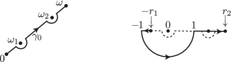
Figure 6: Convolution of aligned poles.

In all cases, there are paths from $0$ to $\omega_{1}+\omega_{2}$ which avoid $\omega_{1}$ and $\omega_{2}$ and which are not paths of analytic continuation for $\hat{\chi}$. This example thus shows that $\hat{\mathscr{R}}_{\{\omega_{1},\omega_{2}\}}$ is not stable under convolution: it contains $\hat{\varphi}$ and $\hat{\psi}$ but not $\hat{\varphi}*\hat{\psi}$.

Now, whenever $\Omega$ is not stable under addition, one can find $\omega_{1},\omega_{2}\in\Omega$ such that $\omega_{1}+\omega_{2}\notin\Omega$ and the previous example then yields $\hat{\varphi},\hat{\psi}\in\hat{\mathscr{R}}_{\Omega}$ with $\hat{\varphi}*\hat{\psi}\notin\hat{\mathscr{R}}_{\Omega}$.

21 Analytic continuation of a convolution product: the general case

21.1  The main result of this section is

Theorem 21.1.

Let $\Omega$ be a non-empty closed discrete subset of $\mathbb{C}$. Then the space $\hat{\mathscr{R}}_{\Omega}$ is stable under convolution if and only if $\Omega$ is stable under addition.

The necessary and sufficient condition on $\Omega$ is satisfied by the typical examples $\mathbb{Z}$ or $2\pi{\mathrm{i}}\mathbb{Z}$, but also by $\mathbb{N}^{*}$, $\mathbb{Z}+{\mathrm{i}}\mathbb{Z}$, $\mathbb{N}^{*}+{\mathrm{i}}\mathbb{N}$ or $\{m+n\sqrt{2}\mid m,n\in\mathbb{N}^{*}\}$ for instance. An immediate consequence of Theorem 21.1 is

Corollary 21.2.

Let $\Omega$ be a non-empty closed discrete subset of $\mathbb{C}$. Then the space $\tilde{\mathscr{R}}_{\Omega}$ of $\Omega$-resurgent formal series is a subalgebra of $\mathbb{C}[[z^{-1}]]$ if and only if $\Omega$ is stable under addition.

The necessity of the condition on $\Omega$ was proved in Section 20. In the rest of this section we shall prove that the condition is sufficient. However we shall restrict ourselves to the case where $0\in\Omega$, because this will allow us to give a simpler proof. The reader is referred to [Sau13] for the proof in the general case.

21.2  We thus fix $\Omega$ closed, discrete, containing $0$ and stable under addition. We begin with a new definition (see Figure 7):

Definition 21.3.

A continuous map $H\colon\thinspace I\times J\to\mathbb{C}$, where $I=[0,1]$ and $J$ is a compact interval of $\mathbb{R}$, is called a symmetric $\Omega$-homotopy if, for each $t\in J$,

$$s\in I\mapsto H_{t}(s)\coloneqq H(s,t)$$

defines a path which satisfies

1. $H_{t}(0)=0$,

2. $H_{t}\big{(}(0,1]\big{)}\subset\mathbb{C}\setminus\Omega$,

3. $H_{t}(1)-H_{t}(s)=H_{t}(1-s)$ for every $s\in I$.

We then call endpoint path of $H$ the path

$${\Gamma}_{H}\colon\thinspace t\in J\mapsto H_{t}(1).$$

Writing $J=[a,b]$, we call $H_{a}$ (resp. $H_{b}$) the initial path of $H$ (resp. its final path).

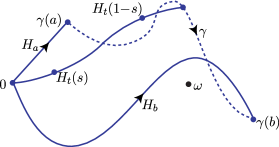
Figure 7: Symmetric $\Omega$-homotopy ($H_{a}=$ initial path, $H_{b}=$ final path, $\gamma=$ endpoint path ${\Gamma}_{H}$).

The first two conditions imply that each path $H_{t}$ is a path of analytic continuation for any $\hat{\varphi}\in\hat{\mathscr{R}}_{\Omega}$, in view of Remark 18.3.

We shall use the notation $H_{t|s}$ for the truncated paths $(H_{t})_{|[0,s]}$, $s\in I$, $t\in J$ (analogously to what we did when commenting Lemma 19.1). Here is a technical statement we shall use:

Lemma 21.4.

For a symmetric $\Omega$-homotopy $H$ defined on $I\times J$, there exists $\delta>0$ such that, for any $\hat{\varphi}\in\hat{\mathscr{R}}_{\Omega}$ and $(s,t)\in I\times J$, the radius of convergence of the holomorphic germ $\operatorname{cont}_{H_{t|s}}\hat{\varphi}$ at $H_{t}(s)$ is at least $\delta$.

Proof.

Let $\rho={\rho(\Omega)}$ (cf. Remark 18.3). Consider

$$U\coloneqq\big{\{}\,(s,t)\in I\times J\mid H\big{(}[0,s]\times\{t\}\big{)}\subset\mathbb{D}_{\rho/2}\,\},\qquad K\coloneqq I\times J\setminus U.$$

Writing $K=\big{\{}\,(s,t)\in I\times J\mid\exists s^{\prime}\in[0,s]\;\text{s.t.}\;H(s^{\prime},t)\in\mathbb{C}\setminus\mathbb{D}_{\rho/2}\,\}$, we see that $K$ is a compact subset of $I\times J$ which is contained in $(0,1]\times J$. Thus $H(K)$ is a compact subset of $\mathbb{C}\setminus\Omega$, and $\delta\coloneqq\min\big{\{}\operatorname{dist}\big{(}H(K),\Omega\big{)},\rho/2\big{\}}>0$. Now, for any $s$ and $t$,

1. either $(s,t)\in U$, then the truncated path $H_{t|s}$ lies in $\mathbb{D}_{\rho/2}$, hence $\operatorname{cont}_{H_{t|s}}\hat{\varphi}$ is a holomorphic germ at $H_{t}(s)$ with radius of convergence $\geq\delta$;

2. or $(s,t)\in K$, and then $\operatorname{dist}(H_{t}(s),\Omega)\geq\delta$, which yields the same conclusion for the germ $\operatorname{cont}_{H_{t|s}}\hat{\varphi}$.

∎

The third condition in Definition 21.3 means that each path $H_{t}$ is symmetric with respect to its midpoint $\frac{1}{2}H_{t}(1)$. Here is the motivation behind this requirement:

Lemma 21.5.

Let $\gamma\colon\thinspace[0,1]\to\mathbb{C}\setminus\Omega$ be a path such that $\gamma(0)\in\mathbb{D}_{\rho(\Omega)}$ (cf. Remark 18.3). If there exists a symmetric $\Omega$-homotopy whose endpoint path coincides with $\gamma$ and whose initial path is contained in $\mathbb{D}_{\rho(\Omega)}$, then any convolution product $\hat{\varphi}*\hat{\psi}$ with $\hat{\varphi},\hat{\psi}\in\hat{\mathscr{R}}_{\Omega}$ can be analytically continued along $\gamma$.

Proof.

We assume that $\gamma={\Gamma}_{H}$ with a symmetric $\Omega$-homotopy $H$ defined on $I\times J$. Let $\hat{\varphi},\hat{\psi}\in\hat{\mathscr{R}}_{\Omega}$ and, for $t\in J$, consider the formula

$$\hat{\chi}_{t}({\zeta})=\int_{H_{t}}\hat{\varphi}(\xi)\hat{\psi}({\zeta}-\xi)\,{\mathrm{d}}\xi+\int_{\gamma(t)}^{\zeta}\hat{\varphi}(\xi)\hat{\psi}({\zeta}-\xi)\,{\mathrm{d}}\xi$$ (106)

(recall that $\gamma(t)=H_{t}(1)$). We shall check that $\hat{\chi}_{t}$ is a well-defined holomorphic germ at $\gamma(t)$ and that it provides the analytic continuation of $\hat{\varphi}*\hat{\psi}$ along $\gamma$.

a) The idea is that when $\xi$ moves along $H_{t}$, $\xi=H_{t}(s)$ with $s\in I$, we can use for “$\hat{\varphi}(\xi)$” the analytic continuation of $\hat{\varphi}$ along the truncated path $H_{t|s}$; correspondingly, if ${\zeta}$ is close to $\gamma(t)$, then ${\zeta}-\xi$ is close to $\gamma(t)-\xi=H_{t}(1)-H_{t}(s)=H_{t}(1-s)$, thus for “$\hat{\psi}({\zeta}-\xi)$” we can use the analytic continuation of $\hat{\psi}$ along $H_{t|1-s}$. In other words, setting ${\zeta}=\gamma(t)+{\sigma}$, we wish to interpret (106) as

$$\hat{\chi}_{t}(\gamma(t)+{\sigma})\coloneqq\int_{0}^{1}(\operatorname{cont}_{H_{t|s}}\hat{\varphi})(H_{t}(s))(\operatorname{cont}_{H_{t|1-s}}\hat{\psi})(H_{t}(1-s)+{\sigma})H_{t}^{\prime}(s)\,{\mathrm{d}}s\\ +\int_{0}^{1}(\operatorname{cont}_{H_{t}}\hat{\varphi})(\gamma(t)+u{\sigma})\hat{\psi}((1-u){\sigma}){\sigma}\,{\mathrm{d}}u$$ (107)

(in the last integral, we have performed the change variable $\xi=\gamma(t)+u{\sigma}$; it is the germ of $\hat{\psi}$ at the origin that we use there).

Lemma 21.4 provides $\delta>0$ such that, by regular dependence of the integrals upon the parameter ${\sigma}$, the right-hand side of (107) is holomorphic for $|{\sigma}|<\delta$. We thus have a family of analytic elements $(\hat{\chi}_{t},D_{t})$, $t\in J$, with $D_{t}\coloneqq\{\,{\zeta}\in\mathbb{C}\mid|{\zeta}-\gamma(t)|<\delta\,\}$.

b) For $t$ small enough, the path $H_{t}$ is contained in $\mathbb{D}_{\rho(\Omega)}$ which is open and simply connected; then, for $|{\zeta}|$ small enough, the line segment $[0,{\zeta}]$ and the concatenation of $H_{t}$ and $[\gamma(t),{\zeta}]$ are homotopic in $\mathbb{D}_{\rho(\Omega)}$, hence the Cauchy theorem implies $\hat{\chi}_{t}({\zeta})=\hat{\varphi}*\hat{\psi}({\zeta})$.

c) By uniform continuity, there exists ${\varepsilon}>0$ such that, for any $t_{0},t\in J$,

$$|t-t_{0}|\leq{\varepsilon}\quad\Longrightarrow\quad|H_{t}(s)-H_{t_{0}}(s)|<\delta/2\quad\text{for all $s\in I$}.$$ (108)

To complete the proof, we check that, for any $t_{0},t$ in $J$ such that $t_{0}\leq t\leq t_{0}+{\varepsilon}$, we have $\hat{\chi}_{t_{0}}\equiv\hat{\chi}_{t}$ in $D\big{(}\gamma(t_{0}),\delta/2)$ (which is contained in $D_{t_{0}}\cap D_{t}$).

Let $t_{0},t\in J$ be such that $t_{0}\leq t\leq t_{0}+{\varepsilon}$ and let ${\zeta}\in D\big{(}\gamma(t_{0}),\delta/2)$. By Lemma 21.4 and (108), we have for every $s\in I$

$$\operatorname{cont}_{H_{t|s}}\hat{\varphi}\big{(}H_{t}(s)\big{)}=\operatorname{cont}_{H_{t_{0}|s}}\hat{\varphi}\big{(}H_{t}(s)\big{)},$$

$$\operatorname{cont}_{H_{t|1-s}}\hat{\psi}\big{(}{\zeta}-H_{t}(s)\big{)}=\operatorname{cont}_{H_{t_{0}|1-s}}\hat{\psi}\big{(}{\zeta}-H_{t}(s)\big{)}$$

(for the latter identity, write ${\zeta}-H_{t}(s)=H_{t}(1-s)+{\zeta}-\gamma(t)=H_{t_{0}}(1-s)+{\zeta}-\gamma(t_{0})+H_{t_{0}}(s)-H_{t}(s)$, thus this point belongs to $D\big{(}H_{t}(1-s),\delta)\cap D\big{(}H_{t_{0}}(1-s),\delta)$). Moreover, $[\gamma(t),{\zeta}]\subset D\big{(}\gamma(t_{0}),\delta/2)$ by convexity, hence $\operatorname{cont}_{H_{t}}\hat{\varphi}\equiv\operatorname{cont}_{H_{t_{0}}}\hat{\varphi}$ on this line segment, and we can write

$$\hat{\chi}_{t}({\zeta})=\int_{0}^{1}(\operatorname{cont}_{H_{t_{0}|s}}\hat{\varphi})(H_{t}(s))(\operatorname{cont}_{H_{t_{0}|1-s}}\hat{\psi})({\zeta}-H_{t}(s))H_{t}^{\prime}(s)\,{\mathrm{d}}s\\ +\int_{\gamma(t)}^{\zeta}(\operatorname{cont}_{H_{t_{0}}}\hat{\varphi})(\xi)\hat{\psi}({\zeta}-\xi)\,{\mathrm{d}}\xi.$$

We then get $\hat{\chi}_{t_{0}}({\zeta})=\hat{\chi}_{t}({\zeta})$ from the Cauchy theorem by means of the homotopy induced by $H$ between the concatenation of $H_{t_{0}}$ and $[\gamma(t_{0}),{\zeta}]$ and the concatenation of $H_{t}$ and $[\gamma(t),{\zeta}]$. ∎

Remark 21.6.

With the notation of Definition 21.3, when the initial path $H_{a}$ is a line segment contained in $\mathbb{D}_{\rho(\Omega)}$, the final path $H_{b}$ is what Écalle calls a “symmetrically contractible path” in [Eca81]. The proof of Lemma 21.5 shows that the analytic continuation of $\hat{\varphi}*\hat{\psi}$ until the endpoint $H_{b}(1)={\Gamma}_{H}(b)$ can be computed by the usual integral taken over $H_{b}$:

$$\operatorname{cont}_{\gamma}(\hat{\varphi}*\hat{\psi})({\zeta})=\int_{H_{b}}\hat{\varphi}(\xi)\hat{\psi}({\zeta}-\xi)\,{\mathrm{d}}\xi,\qquad\gamma={\Gamma}_{H},\enspace{\zeta}=\gamma(b)$$ (109)

(with appropriate interpretation, as in (107)). However, it usually cannot be computed as the same integral over $\gamma={\Gamma}_{H}$ itself, even when the latter integral is well-defined).

21.3  In view of Lemma 21.5, the proof of Theorem 21.1 will be complete if we prove the following purely geometric result:

Lemma 21.7.

For any path $\gamma\colon\thinspace I=[0,1]\to\mathbb{C}\setminus\Omega$ such that $\gamma(0)\in\mathbb{D}^{*}_{\rho(\Omega)}$, there exists a symmetric $\Omega$-homotopy $H$ on $I\times I$ whose endpoint path is $\gamma$ and whose initial path is a line segment, i.e. ${\Gamma}_{H}=\gamma$ and $H_{0}(s)\equiv s\gamma(0)$.

Proof.

Assume that $\gamma$ is given as in the hypothesis of Lemma 21.7. We are looking for a symmetric $\Omega$-homotopy whose initial path is imposed: it must be

$$s\in I\mapsto H_{0}(s)\coloneqq s\gamma(0),$$

which satisfies the three requirements of Definition 21.3 at $t=0$:

1. $H_{0}(0)=0$,

2. $H_{0}\big{(}(0,1]\big{)}\subset\mathbb{C}\setminus\Omega$,

3. $H_{0}(1)-H_{0}(s)=H_{0}(1-s)$ for every $s\in I$.

The idea is to define a family of maps $(\Psi_{t})_{t\in[0,1]}$ so that

$$H_{t}(s)\coloneqq\Psi_{t}\big{(}H_{0}(s)\big{)},\qquad s\in I,$$ (110)

yield the desired homotopy. For that, it is sufficient that $(t,{\zeta})\in[0,1]\times\mathbb{C}\mapsto\Psi_{t}({\zeta})$ be continuously differentiable (for the structure of real two-dimensional vector space of $\mathbb{C}$), $\Psi_{0}=\operatorname{id}$ and, for each $t\in[0,1]$,

1. $\Psi_{t}(0)=0$,

2. $\Psi_{t}(\mathbb{C}\setminus\Omega)\subset\mathbb{C}\setminus\Omega$,

3. $\Psi_{t}\big{(}\gamma(0)-{\zeta}\big{)}=\Psi_{t}\big{(}\gamma(0)\big{)}-\Psi_{t}({\zeta})$ for all ${\zeta}\in\mathbb{C}$,

4. $\Psi_{t}\big{(}\gamma(0)\big{)}=\gamma(t)$.

In fact, the properties (i’)–(iv’) ensure that any initial path $H_{0}$ satisfying (i)–(iii) and ending at $\gamma(0)$ produces through (110) a symmetric $\Omega$-homotopy whose endpoint path is $\gamma$. Consequently, we may assume without loss of generality that $\gamma$ is $C^{1}$ on $[0,1]$ (then, if $\gamma$ is only piecewise $C^{1}$, we just need to concatenate the symmetric $\Omega$-homotopies associated with the various pieces).

The maps $\Psi_{t}$ will be generated by the flow of a non-autonomous vector field $X({\zeta},t)$ associated with $\gamma$ that we now define. We view $(\mathbb{C},|\,\cdot\,|)$ as a real $2$-dimensional Banach space and pick a $C^{1}$ function $\eta\colon\thinspace\mathbb{C}\to[0,1]$ such that

$$\{\,{\zeta}\in\mathbb{C}\mid\eta({\zeta})=0\,\}=\Omega.$$

Observe that $D({\zeta},t)\coloneqq\eta({\zeta})+\eta\big{(}\gamma(t)-{\zeta}\big{)}$ defines a $C^{1}$ function of $({\zeta},t)$ which satisfies

$$D({\zeta},t)>0\quad\text{for all ${\zeta}\in\mathbb{C}$ and $t\in[0,1]$}$$

because $\Omega$ is stable under addition; indeed, $D({\zeta},t)=0$ would imply ${\zeta}\in\Omega$ and $\gamma(t)-{\zeta}\in\Omega$, hence $\gamma(t)\in\Omega$, which would contradict our assumptions. Therefore, the formula

$$X({\zeta},t)\coloneqq\frac{\eta({\zeta})}{\eta({\zeta})+\eta\big{(}\gamma(t)-{\zeta}\big{)}}\gamma^{\prime}(t)$$ (111)

defines a non-autonomous vector field, which is continuous in $({\zeta},t)$ on $\mathbb{C}\times[0,1]$, $C^{1}$ in ${\zeta}$ and has its partial derivatives continuous in $({\zeta},t)$. The Cauchy-Lipschitz theorem on the existence and uniqueness of solutions to differential equations applies to $\frac{{\mathrm{d}}{\zeta}}{{\mathrm{d}}t}=X({\zeta},t)$: for every ${\zeta}\in\mathbb{C}$ and $t_{0}\in[0,1]$ there is a unique solution $t\mapsto\Phi^{t_{0},t}({\zeta})$ such that $\Phi^{t_{0},t_{0}}({\zeta})={\zeta}$. The fact that the vector field $X$ is bounded implies that $\Phi^{t_{0},t}({\zeta})$ is defined for all $t\in[0,1]$ and the classical theory guarantees that $(t_{0},t,{\zeta})\mapsto\Phi^{t_{0},t}({\zeta})$ is $C^{1}$ on $[0,1]\times[0,1]\times\mathbb{C}$.

Let us set $\Psi_{t}\coloneqq\Phi^{0,t}$ for $t\in[0,1]$ and check that this family of maps satisfies (i’)–(iv’). We have

$$X(\omega,t)=0\quad\text{for all $\omega\in\Omega$,}$$ (112)

$$X\big{(}\gamma(t)-{\zeta},t\big{)}=\gamma^{\prime}(t)-X({\zeta},t)\quad\text{for all ${\zeta}\in\mathbb{C}$}$$ (113)

for all $t\in[0,1]$ (by the very definition of $X$). Therefore

• (i’) and (ii’) follow from (112) which yields $\Phi^{t_{0},t}(\omega)=\omega$ for every $t_{0}$ and $t$, whence $\Psi_{t}(0)=0$ since $0\in\Omega$, and from the non-autonomous flow property $\Phi^{t,0}\circ\Phi^{0,t}=\operatorname{id}$ (hence $\Psi_{t}({\zeta})=\omega$ implies ${\zeta}=\Phi^{t,0}(\omega)=\omega$);

• (iv’) follows from the fact that $X\big{(}\gamma(t),t\big{)}=\gamma^{\prime}(t)$, by (112) and (113) with ${\zeta}=0$, using again that $0\in\Omega$, hence $t\mapsto\gamma(t)$ is a solution of $X$;

• (iii’) follows from (113): for any solution $t\mapsto{\zeta}(t)$, the curve $t\mapsto\xi(t)\coloneqq\gamma(t)-{\zeta}(t)$ satisfies $\xi(0)=\gamma(0)-{\zeta}(0)$ and $\xi^{\prime}(t)=\gamma^{\prime}(t)-X\big{(}{\zeta}(t),t\big{)}=X\big{(}\xi(t),t\big{)}$, hence it is a solution: $\xi(t)=\Psi_{t}\big{(}\gamma(0)-{\zeta}(0)\big{)}$.

As explained above, formula (110) thus produces the desired symmetric $\Omega$-homotopy. ∎

21.4  Note on this section: The presentation we adopted is influenced by [CNP93] (the example of Section 20 is taken from this book). Lemma 21.7, which is the key to the proof of Theorem 21.1 and which essentially relies on the use of the flow of the non-autonomous vector field (111), arose as an attempt to understand a related but more complicated (somewhat obscure!) construction which can be found in an appendix of [CNP93]. See [Eca81] and [Ou10] for other approaches to the stability under convolution of the space of resurgent functions.

For the proof of Lemma 21.7, according to [Eca81] and [CNP93], one can visualize the realization of a given path $\gamma$ as the enpoint path ${\Gamma}_{H}$ of a symmetric $\Omega$-homotopy as follows: Let a point ${\zeta}=\gamma(t)$ move along $\gamma$ (as $t$ varies from $0$ to $1$) and remain connected to $0$ by an extensible thread, with moving nails pointing downwards at each point of ${\zeta}-\Omega$, while fixed nails point upwards at each point of $\Omega$ (imagine for instance that the first nails are fastened to a moving rule and the last ones to a fixed rule). As $t$ varies, the thread is progressively stretched but it has to meander between the nails. The path $H_{1}$ used as integration path for $\operatorname{cont}_{\gamma}(\hat{\varphi}*\hat{\psi})(\gamma(1))$ in formula (109) is given by the thread in its final form, when ${\zeta}$ has reached the extremity of $\gamma$; the paths $H_{t}$ correspond to the thread at intermediary stages. See Figure 8 (or Figure 5 of [Sau06]). The point is that none of the moving nails ${\zeta}-\omega^{\prime}\in{\zeta}-\Omega$ will ever collide with a fixed nail $\omega^{\prime\prime}\in\Omega$ because we assumed that $\gamma$ avoids $\{\omega^{\prime}+\omega^{\prime\prime}\}\subset\Omega$.

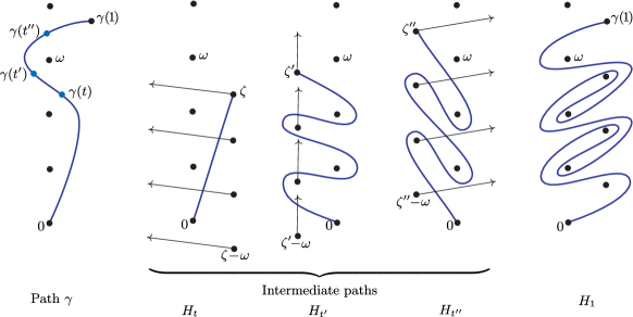
Figure 8: From $\gamma$ to the integration path $H_{1}$ used for $\operatorname{cont}_{\gamma}(\hat{\varphi}*\hat{\psi})(\gamma(1))$.

21.5  Asymmetric version of the result. Theorem 21.1 admits a useful generalization, concerning the convolution product of two resurgent germs which do not belong to the same space of $\Omega$-continuable germs:

Theorem 21.8.

Let $\Omega_{1}$ and $\Omega_{2}$ be non-empty closed discrete subsets of $\mathbb{C}$. Let

$$\Omega\coloneqq\Omega_{1}\cup\Omega_{2}\cup(\Omega_{1}+\Omega_{2}),$$

where $\Omega_{1}+\Omega_{2}\coloneqq\{\,\omega_{1}+\omega_{2}\mid\omega_{1}\in\Omega_{1},\;\omega_{2}\in\Omega_{2}\,\}$. If $\Omega$ is closed and discrete, then

$$\hat{\varphi}\in\hat{\mathscr{R}}_{\Omega_{1}}\enspace\text{and}\enspace\hat{\psi}\in\hat{\mathscr{R}}_{\Omega_{2}}\quad\Longrightarrow\quad\hat{\varphi}*\hat{\psi}\in\hat{\mathscr{R}}_{\Omega}.$$

We shall content ourselves with giving hints about the proof when both $\Omega_{1}$ and $\Omega_{2}$ are assumed to contain $0$, in which case

$$\Omega=\Omega_{1}+\Omega_{2}$$

since both $\Omega_{1}$ and $\Omega_{2}$ are contained in $\Omega_{1}+\Omega_{2}$ (the general case is obtained by adapting the arguments of [Sau13]). Assuming this, we generalize Definition 21.3 and Lemma 21.5:

Definition 21.9.

A continuous map $H\colon\thinspace I\times J\to\mathbb{C}$, where $I=[0,1]$ and $J$ is a compact interval of $\mathbb{R}$, is called an $(\Omega_{1},\Omega_{2})$-homotopy if, for each $t\in J$, the paths $s\in I\mapsto H_{t}(s)\coloneqq H(s,t)$ and $s\in I\mapsto H^{*}_{t}(s)\coloneqq H_{t}(1)-H_{t}(1-s)$ satisfy

1. $H_{t}(0)=0$,

2. $H_{t}\big{(}(0,1]\big{)}\subset\mathbb{C}\setminus\Omega_{1}$,

3. $H^{*}_{t}\big{(}(0,1]\big{)}\subset\mathbb{C}\setminus\Omega_{2}$.

We then call $t\in J\mapsto H_{t}(1)$ the endpoint path of $H$.

Lemma 21.10.

Let $\gamma\colon\thinspace[0,1]\to\mathbb{C}\setminus\Omega$ be a path such that $\gamma(0)\in\mathbb{D}_{\rho(\Omega_{1})}\cap\mathbb{D}_{\rho(\Omega_{2})}$. Suppose that there exists an $(\Omega_{1},\Omega_{2})$-homotopy whose endpoint path coincides with $\gamma$ and such that $H_{0}(I)\subset\mathbb{D}_{\rho(\Omega_{1})}$ and $H^{*}_{0}(I)\subset\mathbb{D}_{\rho(\Omega_{2})}$. Then any convolution product $\hat{\varphi}*\hat{\psi}$ with $\hat{\varphi}\in\hat{\mathscr{R}}_{\Omega_{1}}$ and $\hat{\psi}\in\hat{\mathscr{R}}_{\Omega_{2}}$ can be analytically continued along $\gamma$.

Idea of the proof of Lemma 21.10.

Mimick the proof of Lemma 21.5, replacing the right-hand side of (107) with

$$\int_{0}^{1}(\operatorname{cont}_{H_{t|s}}\hat{\varphi})(H_{t}(s))(\operatorname{cont}_{H^{*}_{t|1-s}}\hat{\psi})(H^{*}_{t}(1-s)+{\sigma})H_{t}^{\prime}(s)\,{\mathrm{d}}s\\ +\int_{0}^{1}(\operatorname{cont}_{H_{t}}\hat{\varphi})(\gamma(t)+u{\sigma})\hat{\psi}((1-u){\sigma}){\sigma}\,{\mathrm{d}}u$$

and showing that this expression is the value at $\gamma(t)+{\sigma}$ of a holomorphic germ, which is $\operatorname{cont}_{\gamma|t}(\hat{\varphi}*\hat{\psi})$. ∎

To conclude the proof of Theorem 21.8, it is thus sufficient to show

Lemma 21.11.

For any path $\gamma\colon\thinspace[0,1]\to\mathbb{C}$ such that $\gamma(0)\in\mathbb{D}^{*}_{\rho(\Omega_{1})}\cap\mathbb{D}^{*}_{\rho(\Omega_{2})}$ and $\gamma\big{(}(0,1]\big{)}\subset\mathbb{C}\setminus\Omega$, there exists an $(\Omega_{1},\Omega_{2})$-homotopy $H$ on $I\times[0,1]$ whose endpoint path is $\gamma$ and such that $H_{0}(s)\equiv s\gamma(0)$.

Indeed, if this lemma holds true, then all such paths $\gamma$ will be, by virtue of Lemma 21.10, paths of analytic continuation for our convolution products $\hat{\varphi}*\hat{\psi}$, which is the content of Theorem 21.8.

Idea of the proof of Lemma 21.11.

It is sufficient to construct a family of maps $(\Psi_{t})_{t\in[0,1]}$ such that $(t,{\zeta})\in[0,1]\times\mathbb{C}\mapsto\Psi_{t}({\zeta})\in\mathbb{C}$ be continuously differentiable (for the structure of real two-dimensional vector space of $\mathbb{C}$), $\Psi_{0}=\operatorname{id}$ and, for each $t\in[0,1]$,

1. $\Psi_{t}(0)=0$,

2. $\Psi_{t}(\mathbb{C}\setminus\Omega_{1})\subset\mathbb{C}\setminus\Omega_{1}$,

3. the map ${\zeta}\in\mathbb{C}\mapsto\Psi^{*}_{t}({\zeta})\coloneqq\gamma(t)-\Psi_{t}({\zeta})$ satisfies $\Psi^{*}_{t}(\mathbb{C}\setminus\Omega_{2})\subset\mathbb{C}\setminus\Omega_{2}$,

4. $\Psi_{t}\big{(}\gamma(0)\big{)}=\gamma(t)$.

Indeed, the formula $H_{t}(s)\coloneqq\Psi_{t}\big{(}s\gamma(0)\big{)}$ then yields the desired homotopy, with $H^{*}_{t}(s)=\Psi^{*}_{t}\big{(}(1-s)\gamma(0)\big{)}$.

As in the proof of Lemma 21.7, the maps $\Psi_{t}$ will be generated by the flow of a non-autonomous vector field associated with $\gamma$. We view $(\mathbb{C},|\,\cdot\,|)$ as a real $2$-dimensional Banach space and pick $C^{1}$ functions $\eta_{1},\eta_{2}\colon\thinspace\mathbb{C}\to[0,1]$ such that

$$\{\,{\zeta}\in\mathbb{C}\mid\eta_{j}({\zeta})=0\,\}=\Omega_{j},\qquad j=1,2.$$

Observe that $D({\zeta},t)\coloneqq\eta_{1}({\zeta})+\eta_{2}\big{(}\gamma(t)-{\zeta}\big{)}$ defines a $C^{1}$ function of $({\zeta},t)$ which satisfies

$$D({\zeta},t)>0\quad\text{for all ${\zeta}\in\mathbb{C}$ and $t\in[0,1]$,}$$

since $D({\zeta},t)=0$ would imply ${\zeta}\in\Omega_{1}$ and $\gamma(t)-{\zeta}\in\Omega_{2}$, hence $\gamma(t)\in\Omega_{1}+\Omega_{2}$, which would contradict our assumptions. Therefore, the formula

$$X({\zeta},t)\coloneqq\frac{\eta_{1}({\zeta})}{\eta_{1}({\zeta})+\eta_{2}\big{(}\gamma(t)-{\zeta}\big{)}}\gamma^{\prime}(t)$$ (114)

defines a non-autonomous vector field and the Cauchy-Lipschitz theorem applies to $\frac{{\mathrm{d}}{\zeta}}{{\mathrm{d}}t}=X({\zeta},t)$: for every ${\zeta}\in\mathbb{C}$ and $t_{0}\in[0,1]$ there is a unique solution $t\in[0,1]\mapsto\Phi_{X}^{t_{0},t}({\zeta})$ such that $\Phi_{X}^{t_{0},t_{0}}({\zeta})={\zeta}$; the flow map $(t_{0},t,{\zeta})\mapsto\Phi_{X}^{t_{0},t}({\zeta})$ is $C^{1}$ on $[0,1]\times[0,1]\times\mathbb{C}$.

Setting $\Psi_{t}\coloneqq\Phi_{X}^{0,t}$ for $t\in[0,1]$, one can check that this family of maps satisfies (i’)–(iv’) by mimicking the arguments in the proof of Lemma 21.7 and using the fact that the corresponding family of maps $(\Psi^{*}_{t})$ in (iii’) can be obtained from the identity

$$\gamma(t)-\Phi_{X}^{0,t}({\zeta})=\Phi_{X^{*}}^{0,t}\big{(}\gamma(0)-{\zeta}\big{)},$$

where we denote by $(t_{0},t,{\zeta})\mapsto\Phi_{X^{*}}^{t_{0},t}({\zeta})$ the flow map of the non-autonomous vector field

$$X^{*}({\zeta},t)\coloneqq\gamma^{\prime}(t)-X\big{(}\gamma(t)-{\zeta},t\big{)}=\frac{\eta_{2}({\zeta})}{\eta_{1}\big{(}\gamma(t)-{\zeta}\big{)}+\eta_{2}({\zeta})}\gamma^{\prime}(t).$$

∎

22 Non-linear operations with resurgent formal series

From now on, we give ourselves a non-empty closed discrete subset $\Omega$ of $\mathbb{C}$ which is stable under addition.

We already mentioned the stability of $\tilde{\mathscr{R}}_{\Omega}$ under certain linear difference/differential operators in Lemma 18.6. Now, with our assumption that $\Omega$ is stable under addition, we can obtain the stability of $\Omega$-resurgent formal series under the non-linear operations which were studied in Sections 13 and 17. However this requires quantitative estimates for iterated convolutions whose proof is beyond the scope of the present text, we thus quote without proof the following

Lemma 22.1.

Let $\gamma$ be a path of $\mathbb{C}\setminus\Omega$ starting from a point ${\zeta}_{0}\in\mathbb{D}_{\rho(\Omega)}$ and ending at a point ${\zeta}_{1}$. Let $R>0$ be such that $\overline{D({\zeta}_{1},R)}\subset\mathbb{C}\setminus\Omega$. Then there exist a positive number $L$ and a set $\mathscr{C}$ of paths parametrized by $[0,1]$ and contained in $\mathbb{D}_{L}\setminus\Omega$ such that, for every $\hat{\varphi}\in\hat{\mathscr{R}}_{\Omega}$, the number

$$\lVert\hat{\varphi}\rVert_{\mathscr{C}}\coloneqq\sup_{\tilde{\gamma}\in\mathscr{C}}\left\lvert\operatorname{cont}_{\tilde{\gamma}}\hat{\varphi}\big{(}\tilde{\gamma}(1)\big{)}\right\rvert$$

is finite, and there exist $A,B>0$ such that, for every $k\geq 1$ and $\hat{\varphi},\hat{\psi}\in\hat{\mathscr{R}}_{\Omega}$, the iterated convolution products

$$\hat{\varphi}^{*k}\coloneqq\underbrace{\hat{\varphi}*\cdots*\hat{\varphi}}_{\text{$k$ factors}}$$

and $\hat{\psi}*\hat{\varphi}^{*k}$ (which admit analytic continuation along $\gamma$, according to Theorem 21.1) satisfy

$$\lvert\operatorname{cont}_{\gamma}\hat{\varphi}^{*k}({\zeta})\rvert \leq A\frac{B^{k}}{k!}\big{(}\lVert\hat{\varphi}\rVert_{\mathscr{C}}\big{)}^{k},$$

$$\lvert\operatorname{cont}_{\gamma}(\hat{\psi}*\hat{\varphi}^{*k})({\zeta})\rvert \leq A\frac{B^{k}}{k!}\lVert\hat{\psi}\rVert_{\mathscr{C}}\big{(}\lVert\hat{\varphi}\rVert_{\mathscr{C}}\big{)}^{k},$$

for every ${\zeta}\in\overline{D({\zeta}_{1},R)}$.

The proof can be found in [Sau14]. Taking this result for granted, we can show

Theorem 22.2.

Suppose that $\tilde{\varphi}(z),\tilde{\psi}(z),\tilde{\chi}(z)\in\tilde{\mathscr{R}}_{\Omega}$ and that $\tilde{\chi}(z)$ has no constant term. Let $H(t)\in\mathbb{C}\{t\}$. Then

$$\tilde{\psi}\circ(\operatorname{id}+\tilde{\varphi})\in\tilde{\mathscr{R}}_{\Omega},\qquad H\circ\tilde{\chi}\in\tilde{\mathscr{R}}_{\Omega}.$$ (115)

Proof.

We can write $\tilde{\varphi}=a+\tilde{\varphi}_{1}$, $\tilde{\psi}=b+\tilde{\psi}_{1}$, where $a,b\in\mathbb{C}$ and $\tilde{\varphi}_{1}$ and $\tilde{\psi}_{1}$ have no constant term. With notations similar to those of the proof of Theorem 13.3, we write the first formal series in (115) as $b+\tilde{\lambda}(z)$ and the second one as $c+\tilde{\mu}(z)$, where $c=H(0)$. Since $\tilde{\lambda}=(T_{a}\tilde{\psi}_{1})\circ(\operatorname{id}+\tilde{\varphi}_{1})$, where $T_{a}\tilde{\psi}_{1}$ is $\Omega$-resurgent (by Lemma 18.6) and has no constant term, we see that it is sufficient to deal with the case $a=b=0$; from now on we thus suppose $\tilde{\varphi}=\tilde{\varphi}_{1}$ and $\tilde{\psi}=\tilde{\psi}_{1}$. Then

$$\tilde{\lambda}=\tilde{\psi}\circ(\operatorname{id}+\tilde{\varphi})=\sum_{k\geq 0}\frac{1}{k!}(\partial^{k}\tilde{\psi})\tilde{\varphi}^{k},\qquad\tilde{\mu}=\sum_{k\geq 1}h_{k}\tilde{\chi}^{k}$$

where $H(t)=c+\sum_{k\geq 1}h_{k}t^{k}$ with $|h_{k}|\leq CD^{k}$ for some $C,D>0$ independent of $k$, and the corresponding formal Borel transforms are

$$\hat{\lambda}=\sum_{k\geq 0}\frac{1}{k!}\big{(}(-{\zeta})^{k}\hat{\psi}\big{)}*\hat{\varphi}^{*k},\qquad\hat{\mu}=\sum_{k\geq 1}h_{k}\hat{\chi}^{*k}.$$

These can be viewed as formally convergent series of elements of $\mathbb{C}[[{\zeta}]]$, in which each term belongs to $\hat{\mathscr{R}}_{\Omega}$ (by virtue of Theorem 21.1). They define holomorphic germs in $\mathbb{D}_{\rho(\Omega)}$ because they can also be seen as normally convergent series of holomorphic functions in any compact disc contained in $\mathbb{D}_{\rho(\Omega)}$ (by virtue of inequalities (79) and (81)).

To conclude, it is sufficient to check that, given a path $\gamma\colon\thinspace[0,1]\to\mathbb{C}\setminus\Omega$ starting in $\mathbb{D}_{\rho(\Omega)}$, for every $t\in[0,1]$ and $R_{t}>0$ such that $\overline{D\big{(}\gamma(t),R_{t}\big{)}}\subset\mathbb{C}\setminus\Omega$ the series of holomorphic functions

$$\sum\frac{1}{k!}\operatorname{cont}_{\gamma_{|[0,t]}}\Big{(}\big{(}(-{\zeta})^{k}\hat{\psi}\big{)}*\hat{\varphi}^{*k}\Big{)}\quad\text{and}\quad\sum h_{k}\operatorname{cont}_{\gamma_{|[0,t]}}\big{(}\hat{\chi}^{*k}\big{)}$$

are normally convergent on $\overline{D\big{(}\gamma(t),R_{t}\big{)}}$ (indeed, this will provide families of analytic elements which analytically continue $\hat{\lambda}$ and $\hat{\mu}$). This follows from Lemma 22.1. ∎

Example 22.1.

In view of Lemma 18.4, since $2\pi{\mathrm{i}}\,\mathbb{Z}$ is stable under addition, this implies that the exponential of the Stirling series $\tilde{\lambda}=\mathrm{e}^{\tilde{\mu}}$ is $2\pi{\mathrm{i}}\,\mathbb{Z}$-resurgent.

Recall that $\tilde{\mathscr{G}}=\operatorname{id}+\mathbb{C}[[z^{-1}]]$ is the topological group of formal tangent-to-identity diffeomorphisms at $\infty$ studied in Section 15.

Definition 22.3.

We call $\Omega$-resurgent tangent-to-identity diffeomorphism any $\tilde{f}=\operatorname{id}+\tilde{\varphi}\in\tilde{\mathscr{G}}$ where $\tilde{\varphi}$ is an $\Omega$-resurgent formal series. We use the notations

$$\tilde{\mathscr{G}}^{\mathrm{RES}}(\Omega)\coloneqq\{\,\tilde{f}=\operatorname{id}+\tilde{\varphi}\mid\tilde{\varphi}\in\tilde{\mathscr{R}}_{\Omega}\,\},\qquad\tilde{\mathscr{G}}^{\mathrm{RES}}_{\sigma}(\Omega)\coloneqq\tilde{\mathscr{G}}^{\mathrm{RES}}(\Omega)\cap\tilde{\mathscr{G}}_{\sigma}\enspace\text{for ${\sigma}\in\mathbb{C}$.}$$

Observe that $\tilde{\mathscr{G}}^{\mathrm{RES}}(\Omega)$ is not a closed subset of $\tilde{\mathscr{G}}$ for the topology which was introduced in Section 15; in fact it is dense, since it contains the subset $\mathscr{G}$ of holomorphic tangent-to-identity germs of diffeomorphisms at $\infty$, which itself is dense in $\tilde{\mathscr{G}}$.

Theorem 22.4.

The set $\tilde{\mathscr{G}}^{\mathrm{RES}}(\Omega)$ is a subgroup of $\tilde{\mathscr{G}}$, the set $\tilde{\mathscr{G}}^{\mathrm{RES}}_{0}(\Omega)$ is a subgroup of $\tilde{\mathscr{G}}_{0}$.

Proof.

The stability under group composition stems from Theorem 22.2, since $(\operatorname{id}+\tilde{\psi})\circ(\operatorname{id}+\tilde{\varphi})=\operatorname{id}+\tilde{\varphi}+\tilde{\psi}\circ(\operatorname{id}+\tilde{\varphi})$.

For the stability under group inversion, we only need to prove

$$\tilde{h}=\operatorname{id}+\tilde{\chi}\in\tilde{\mathscr{G}}^{\mathrm{RES}}(\Omega)\quad\Longrightarrow\quad\tilde{h}^{\circ(-1)}\in\tilde{\mathscr{G}}^{\mathrm{RES}}(\Omega).$$

It is sufficient to prove this when $\tilde{\chi}$ has no constant term, i.e. when $\tilde{h}\in\tilde{\mathscr{G}}^{\mathrm{RES}}_{0}(\Omega)$, since we can always write $\tilde{h}=(\operatorname{id}+\tilde{\chi}_{1})\circ(\operatorname{id}+a)$ with a formal series $\tilde{\chi}_{1}=T_{-a}(-a+\tilde{\chi})\in\tilde{\mathscr{R}}_{\Omega}$ which has no constant term (taking $a=$ constant term of $\tilde{\chi}$ and using Lemma 18.6) and then $\tilde{h}^{\circ(-1)}=(\operatorname{id}+\tilde{\chi}_{1})^{\circ(-1)}-a$.

We thus assume that $\tilde{\chi}=\tilde{\chi}_{1}\in\tilde{\mathscr{R}}_{\Omega}$ has no constant term and apply the Lagrange reversion formula (90) to $\tilde{h}=\operatorname{id}+\tilde{\chi}$. We get $\tilde{h}^{\circ(-1)}=\operatorname{id}-\tilde{\varphi}$ with the Borel transform of $\tilde{\varphi}$ given by

$$\hat{\varphi}=\sum_{k\geq 1}\frac{{\zeta}^{k-1}}{k!}\hat{\chi}^{*k},$$

formally convergent series in $\mathbb{C}[[{\zeta}]]$, in which each term belongs to $\hat{\mathscr{R}}_{\Omega}$. The holomorphy of $\hat{\varphi}$ in $\mathbb{D}_{\rho(\Omega)}$ and its analytic continuation along the paths of $\mathbb{C}\setminus\Omega$ are obtained by invoking inequalities (94) and Lemma 22.1, similarly to what we did at the end of the proof of Theorem 22.2. ∎

Simple singularities

23 Singular points

When the analytic continuation of a holomorphic germ $\raisebox{-0.99025pt}{${\stackrel{{\scriptstyle\raisebox{-0.54247pt}{$\scriptscriptstyle\wedge$}}}{{\varphi}}}$}({\zeta})$ has singularities (i.e. ${\stackrel{{\scriptstyle\raisebox{-0.54247pt}{$\scriptscriptstyle\wedge$}}}{{\varphi}}}$ does not extend to an entire function), its inverse formal Borel transform $\tilde{\varphi}=\mathcal{B}^{-1}\raisebox{-0.99025pt}{${\stackrel{{\scriptstyle\raisebox{-0.54247pt}{$\scriptscriptstyle\wedge$}}}{{\varphi}}}$}$ is a divergent formal series, and the location and the nature of the singularities in the ${\zeta}$-plane influence the growth of the coefficients of $\tilde{\varphi}$. By analysing carefully the singularities of ${\stackrel{{\scriptstyle\raisebox{-0.54247pt}{$\scriptscriptstyle\wedge$}}}{{\varphi}}}$, one may hope to be able to deduce subtler information on $\tilde{\varphi}$ and, if Borel-Laplace summation is possible, on its Borel sums.

Therefore, we shall now develop a theory which allows one to study and manipulate singularities (in the case of isolated singular points).

First, recall the definition of a singular point in complex analysis: given $f$ holomorphic in an open subset $U$ of $\mathbb{C}$, a boundary point $\omega$ of $U$ is said to be a singular point of $f$ if one cannot find an open neighbourhood $V$ of $\omega$, a function $g$ holomorphic in $V$, and an open subset $U^{\prime}$ of $U$ such that $\omega\in\partial U^{\prime}$ and $f_{|U^{\prime}\cap V}=g_{|U^{\prime}\cap V}$.

Thus this notion refers to the imposssibility of extending locally the function: even when restricting to a smaller domain $U^{\prime}$ to which $\omega$ is adherent, we cannot find an analytic continuation in a full neighbourhood of $\omega$. Think of the example of the principal branch of logarithm: it can be defined as the holomorphic function

$$\mathrm{Log\hskip 1.5pt}{\zeta}\coloneqq\int_{1}^{\zeta}\frac{{\mathrm{d}}\xi}{\xi}\quad\text{for ${\zeta}\in U=\mathbb{C}\setminus\mathbb{R}^{-}$.}$$ (116)

Then, for $\omega<0$, one cannot find a holomorphic extension of $f=\mathrm{Log\hskip 1.5pt}$ from $U$ to any larger open set containing $\omega$ (not even a continuous extension!), however such a point $\omega$ is not singular: if we first restrict, say, to the upper half-plane $U^{\prime}\coloneqq\{\mathop{\Im m}\nolimits{\zeta}>0\}$, then we can easily find an analytic continuation of $\mathrm{Log\hskip 1.5pt}_{|U^{\prime}}$ to $U^{\prime}\cup V$, where $V$ is the disc $D(\omega,|\omega|)$: define $g$ by

$$g({\zeta})=\bigg{(}\int_{\gamma}+\int_{\omega}^{\zeta}\bigg{)}\frac{{\mathrm{d}}\xi}{\xi}$$

with any path $\gamma\colon\thinspace[0,1]\to\mathbb{C}$ such that $\gamma(0)=1$, $\gamma\big{(}(0,1)\big{)}\subset U^{\prime}$ and $\gamma(1)=\omega$. In fact, for the function $f=\mathrm{Log\hskip 1.5pt}$, the only singular point is $0$, there is no other local obstacle to analytic continuation, even though there is no holomorphic extension of this function to $\mathbb{C}^{*}$.

If $\omega$ is an isolated singular point for a holomorphic function $f$, we can wonder what kind of singularity occurs at this point. There are certainly many ways for a point to be singular: maybe the function near $\omega$ looks like $\log({\zeta}-\omega)$ (for an appropriate branch of the logarithm), or like a pole $\frac{C}{({\zeta}-\omega)^{m}}$, and the reader can imagine many other singular behaviours (square-root branching $({\zeta}-\omega)^{1/2}$, powers of logarithm $\big{(}\log({\zeta}-\omega)\big{)}^{m}$, iterated logarithms $\log\big{(}\log({\zeta}-\omega)\big{)}$, etc.). The singularity of $f$ at $\omega$ will be defined as an equivalence class modulo regular functions in Section 25. Of course, by translating the variable, we can always assume $\omega=0$. Observe that, in this text, we make a distinction between singular points and singularities (the former being the locations of the latter).

As a preliminary, we need to introduce a few notations in relation with the Riemann surface of the logarithm.

24 The Riemann surface of the logarithm

The Riemann surface of the logarithm $\tilde{\mathbb{C}}$ can be defined topologically (without any reference to the logarithm!) as the universal cover of $\mathbb{C}^{*}$ with base point at $1$. This means that we consider the set $\mathscr{P}$ of all paths $\gamma\colon\thinspace[0,1]\to\mathbb{C}^{*}$ with $\gamma(0)=1$, we put on $\mathscr{P}$ the equivalence relation $\sim$ of “homotopy with fixed endpoints”, i.e.

$$\gamma\sim\gamma_{0}\quad\Longleftrightarrow\quad\exists H\colon\thinspace[0,1]\times[0,1]\to\mathbb{C}^{*}\;\text{continuous, such that $H(0,\cdot\,)=\gamma_{0}$, $H(1,\cdot\,)=\gamma$,}\\[4.30554pt] \text{$H(s,0)=\gamma_{0}(0)$ and $H(s,1)=\gamma_{0}(1)$ for each $s\in[0,1]$,}$$

and we define $\tilde{\mathbb{C}}$ as the set of all equivalence classes,

$$\tilde{\mathbb{C}}\coloneqq\mathscr{P}/\sim.$$

Observe that, if $\gamma\sim\gamma_{0}$, then $\gamma(1)=\gamma_{0}(1)$: the endpoint $\gamma(1)$ does not depend on $\gamma$ but only on its equivalence class $[\gamma]$. We thus get a map

$$\pi\colon\thinspace\tilde{\mathbb{C}}\to\mathbb{C}^{*},\qquad\pi({\zeta})=\gamma(1)\enspace\text{for any $\gamma\in\mathscr{P}$ such that $[\gamma]={\zeta}$}$$

(recall that the other endpoint is the same for all paths $\gamma\in\mathscr{P}$: $\gamma(0)=1$).

Among all the representatives of an equivalence class ${\zeta}\in\tilde{\mathbb{C}}$, there is a canonical one: there exists a unique pair $(r,{\theta})\in(0,+\infty)\times\mathbb{R}$ such that ${\zeta}$ is represented by the concatenation of the paths $t\in[0,1]\mapsto\mathrm{e}^{{\mathrm{i}}t{\theta}}$ and $t\in[0,1]\mapsto\big{(}1+t(r-1)\big{)}\mathrm{e}^{{\mathrm{i}}{\theta}}$. In that situation, we use the notations

$${\zeta}=r\,{\underline{\mathrm{e}}}^{{\mathrm{i}}{\theta}},\qquad r=\lvert{\zeta}\rvert,\qquad{\theta}=\arg{\zeta},$$

so that we can write $\pi(r\,{\underline{\mathrm{e}}}^{{\mathrm{i}}{\theta}})=r\,\mathrm{e}^{{\mathrm{i}}{\theta}}$. Heuristically, one may think of ${\theta}\mapsto{\underline{\mathrm{e}}}^{{\mathrm{i}}{\theta}}$ as of a non-periodic exponential: it keeps track of the number of turns around the origin, not only of the angle ${\theta}$ modulo $2\pi$.

There is a simple way of defining a Riemann surface structure on $\tilde{\mathbb{C}}$. One first defines a Hausdorff topology on $\tilde{\mathbb{C}}$ by taking as a basis $\big{\{}\,\tilde{D}({\zeta},R)\mid{\zeta}\in\tilde{\mathbb{C}},\;0<R<\lvert\pi({\zeta})\rvert\,\big{\}}$, where $\tilde{D}({\zeta},R)$ is the set of the equivalence classes of all paths $\gamma$ obtained as concatenation of a representative of ${\zeta}$ and a line segment starting from $\pi({\zeta})$ and contained in $D(\pi({\zeta}),R)$ (cf. notation (96)). (Exercise: check that this is legitimate, i.e. that $\big{\{}\,\tilde{D}({\zeta},R)\,\big{\}}$ is a collection of subsets of $\tilde{\mathbb{C}}$ which meets the necessary conditions for being the basis of a topology, and check that the resulting topology satisfies the Hausdorff separation axiom.) It is easy to check that, for each basis element, the projection $\pi$ induces a homeomorphism $\pi_{{\zeta},R}\colon\thinspace\tilde{D}({\zeta},R)\to D(\pi({\zeta}),R)$ and that, for each pair of basis elements with non-empty intersection, the transition map $\pi_{{\zeta}^{\prime},R^{\prime}}\circ\pi_{{\zeta},R}^{-1}$ is the identity map on $D(\pi({\zeta}),R)\cap D(\pi({\zeta}^{\prime}),R^{\prime})\subset\mathbb{C}$, hence we get an atlas $\{\pi_{{\zeta},R}\}$ which defines a Riemann surface structure on $\tilde{\mathbb{C}}$, i.e. a $1$-dimensional complex manifold structure (because the identity map is holomorphic!).

Now, why do we call $\tilde{\mathbb{C}}$ the Riemann surface of the logarithm? This is not so apparent in the presentation that was adopted here, but in fact the above construction is related to a more general one, in which one starts with an arbitrary open connected subset $U$ of $\mathbb{C}$ and a holomorphic function $f$ on $U$, and one constructs (by quotienting a certain set of paths) a Riemann surface in which $U$ is embedded and on which $f$ has a holomorphic extension. We shall not give the details, but content ourselves with checking the last property for $U=\mathbb{C}\setminus\mathbb{R}^{-}$ and $f=\mathrm{Log\hskip 1.5pt}$ defined by (116), defining a holomorphic function $\mathscr{L}\colon\thinspace\tilde{\mathbb{C}}\to\mathbb{C}$ and explaining why it deserves to be considered as a holomorphic extension of the logarithm.

We first observe that $\tilde{U}\coloneqq\pi^{-1}(U)$ is an open subset of $\tilde{\mathbb{C}}$ with infinitely many connected components,

$$\tilde{U}_{m}\coloneqq\{\,r\,{\underline{\mathrm{e}}}^{{\mathrm{i}}{\theta}}\in\tilde{\mathbb{C}}\mid r>0,\;2\pi m-\pi<{\theta}<2\pi m+\pi\,\},\qquad m\in\mathbb{Z}.$$

By restriction, the projection $\pi$ induces a biholomorphism

$$\pi_{0}\colon\thinspace\tilde{U}_{0}\xrightarrow{\sim}U$$

(it does so for any $m\in\mathbb{Z}$ but, quite arbitrarily, we choose $m=0$ here). The principal sheet of the Riemann surface of the logarithm is defined to be the set $\tilde{U}_{0}\subset\tilde{\mathbb{C}}$, which is identified to the cut plane $U\subset\mathbb{C}$ by means of $\pi_{0}$.

On the other hand, since the function $\xi\mapsto 1/\xi$ is holomorphic on $\mathbb{C}^{*}$, the Cauchy theorem guarantees that, for any $\gamma\in\mathscr{P}$, the integral $\int_{\gamma}\frac{{\mathrm{d}}\xi}{\xi}$ depends only on the equivalence class $[\gamma]$, we thus get a function

$$\mathscr{L}\colon\thinspace\tilde{\mathbb{C}}\to\mathbb{C},\qquad\mathscr{L}\big{(}[\gamma]\big{)}\coloneqq\int_{\gamma}\frac{{\mathrm{d}}\xi}{\xi}.$$

This function is holomorphic on the whole of $\tilde{\mathbb{C}}$, because its expression in any chart domain $\tilde{D}({\zeta}_{0},R)$ is

$$\mathscr{L}({\zeta})=\mathscr{L}({\zeta}_{0})+\int_{\pi({\zeta}_{0})}^{\pi({\zeta})}\frac{{\mathrm{d}}\xi}{\xi},$$

which is a holomorphic function of $\pi({\zeta})$.

Now, since any ${\zeta}\in\tilde{U}_{0}$ can be represented by a line segment starting from $1$, we have

$$\mathscr{L}_{|\tilde{U}_{0}}=\mathrm{Log\hskip 1.5pt}\circ\pi_{0}.$$

In other words, if we identify $U$ and $\tilde{U}_{0}$ by means of $\pi_{0}$, we can view $\mathscr{L}$ as a holomorphic extension of $\mathrm{Log\hskip 1.5pt}$ to the whole of $\tilde{\mathbb{C}}$.

The function $\mathscr{L}$ is usually denoted $\log$. Notice that $\mathscr{L}(r\,{\underline{\mathrm{e}}}^{{\mathrm{i}}{\theta}})=\ln r+{\mathrm{i}}{\theta}$ for all $r>0$ and ${\theta}\in\mathbb{R}$, and that $\mathscr{L}=\log$ is a biholomorphism $\tilde{\mathbb{C}}\to\mathbb{C}$ (with our notations: $\mathscr{L}^{-1}(x+{\mathrm{i}}y)=\mathrm{e}^{x}\,{\underline{\mathrm{e}}}^{{\mathrm{i}}y}$). Notice also that there is a natural multiplication $(r_{1}\,{\underline{\mathrm{e}}}^{{\mathrm{i}}{\theta}_{1}},r_{2}\,{\underline{\mathrm{e}}}^{{\mathrm{i}}{\theta}_{2}})\mapsto r_{1}r_{2}\,\mathrm{e}^{{\mathrm{i}}({\theta}_{1}+{\theta}_{2})}$ in $\tilde{\mathbb{C}}$, inherited from the addition in $\mathbb{C}$.

25 The formalism of singularities

We are interested in holomorphic functions $f$ for which the origin is locally the only singular point in the following sense:

Definition 25.1.

We say that a function $f$ has spiral continuation around $0$ if it is holomorphic in an open disc $D$ to which $0$ is adherent and, for every $L>0$, there exists $\rho>0$ such that $f$ can be analytically continued along any path of length $\leq L$ starting from $D\cap\mathbb{D}^{*}_{\rho}$ and staying in $\mathbb{D}^{*}_{\rho}$ (recall the notation (97)). See Figure 9.

In the following we shall need to single out one of the connected components of $\pi^{-1}(D)$ in $\tilde{\mathbb{C}}$, but there is no canonical choice in general. (If one of the connected components is contained in the principal sheet of $\tilde{\mathbb{C}}$, we may be tempted to choose this one, but this does not happen when the centre of $D$ has negative real part and we do not want to eliminate a priori this case.) We thus choose ${\zeta}_{0}\in\tilde{\mathbb{C}}$ such that $\pi({\zeta}_{0})$ is the centre of $D$, then the connected component of $\pi^{-1}(D)$ which contains ${\zeta}_{0}$ is a domain $\tilde{D}$ of the form $\tilde{D}({\zeta}_{0},R_{0})$ (notation of the previous section) and this will be the connected component that we single out.

Since $\pi$ induces a biholomorphism $\tilde{D}\xrightarrow{\sim}D$, we can identify $f$ with ${\stackrel{{\scriptstyle\raisebox{-0.69318pt}{$\scriptscriptstyle\vee$}}}{{f}}}\coloneqq f\circ\pi$ viewed as a holomorphic function on $\tilde{D}$. Now, the spiral continuation property implies that ${\stackrel{{\scriptstyle\raisebox{-0.69318pt}{$\scriptscriptstyle\vee$}}}{{f}}}$ extends analytically to a domain of the form

$$\mathcal{V}(h)\coloneqq\{\,{\zeta}=r\,{\underline{\mathrm{e}}}^{{\mathrm{i}}{\theta}}\mid 0<r<h({\theta}),\;{\theta}\in\mathbb{R}\,\}\subset\tilde{\mathbb{C}},$$

with a continuous function $h\colon\thinspace\mathbb{R}\to(0,+\infty)$, but in fact the precise function $h$ is of no interest to us. We are thus led to

Figure 9: The function $f$ is holomorphic in $D$ and has spiral continuation around $0$.

Definition 25.2.

We define the space $\operatorname{ANA}$ of all singular germs as follows: on the set of all pairs $({\stackrel{{\scriptstyle\raisebox{-0.69318pt}{$\scriptscriptstyle\vee$}}}{{f}}},h)$, where $h\colon\thinspace\mathbb{R}\to(0,+\infty)$ is continuous and ${\stackrel{{\scriptstyle\raisebox{-0.69318pt}{$\scriptscriptstyle\vee$}}}{{f}}}\colon\thinspace\mathcal{V}(h)\to\mathbb{C}$ is holomorphic, we put the equivalence relation

$$(\stackrel{{\scriptstyle\raisebox{-0.69318pt}{$\scriptscriptstyle\vee$}}}{{f}}\vphantom{f}_{1},h_{1})\sim(\stackrel{{\scriptstyle\raisebox{-0.69318pt}{$\scriptscriptstyle\vee$}}}{{f}}\vphantom{f}_{2},h_{2})\quad\xLeftrightarrow{\text{\enspace def\enspace}}\quad\stackrel{{\scriptstyle\raisebox{-0.69318pt}{$\scriptscriptstyle\vee$}}}{{f}}\vphantom{f}_{1}\equiv\stackrel{{\scriptstyle\raisebox{-0.69318pt}{$\scriptscriptstyle\vee$}}}{{f}}\vphantom{f}_{2}\;\text{on $\mathcal{V}(h_{1})\cap\mathcal{V}(h_{2})$,}$$

and we define $\operatorname{ANA}$ as the quotient set.

Heuristically, one may think of a singular germ as of a “germ of holomorphic function at the origin of $\tilde{\mathbb{C}}$” (except that $\tilde{\mathbb{C}}$ has no origin!). We shall usually make no notational difference between an element of $\operatorname{ANA}$ and any of its representatives. As explained above, the formula $f={\stackrel{{\scriptstyle\raisebox{-0.69318pt}{$\scriptscriptstyle\vee$}}}{{f}}}\circ\pi$ allows one to identify a singular germ ${\stackrel{{\scriptstyle\raisebox{-0.69318pt}{$\scriptscriptstyle\vee$}}}{{f}}}$ with a function $f$ which has spiral continuation around $0$; however, one must be aware that this presupposes an identification, by means of $\pi$, between a simply connected domain $D$ of $\mathbb{C}^{*}$ (e.g. an open disc) and a subset $\tilde{D}$ of a domain of the form $\mathcal{V}(h)$ (and, given $D$, there are countably many choices for $\tilde{D}$).

Example 25.1.

Suppose that $f$ is holomorphic in the punctured disc $\mathbb{D}_{\rho}^{*}$, for some $\rho>0$; in particular, it is holomorphic in $D=D(\frac{\rho}{2},\frac{\rho}{2})$ and we can apply the above construction. Then, for whatever choice of a connected component of $\pi^{-1}(D)$ in $\tilde{\mathbb{C}}$, we obtain the same ${\stackrel{{\scriptstyle\raisebox{-0.69318pt}{$\scriptscriptstyle\vee$}}}{{f}}}\coloneqq f\circ\pi$ holomorphic in $\mathcal{V}(h)$ with a constant function $h({\theta})\equiv\rho$. The corresponding element of $\operatorname{ANA}$ identifies itself with the Laurent series of $f$ at $0$, which is of the form

$$\sum_{n\in\mathbb{Z}}a_{n}{\zeta}^{n}=S(1/{\zeta})+R({\zeta}),$$ (117)

with $R({\zeta})\coloneqq\sum_{n\geq 0}a_{n}{\zeta}^{n}$ of radius of convergence $\geq\rho$ and $S(\xi)\coloneqq\sum_{n>0}a_{-n}\xi^{n}$ of infinite radius of convergence. Heuristically, the “singularity of $f$” is encoded by the sole term $S(1/{\zeta})$; Definition 25.3 will formalize the idea of discarding the regular term $R({\zeta})$.

Example 25.2.

Suppose that $f$ is of the form $f({\zeta})=\raisebox{-0.99025pt}{${\stackrel{{\scriptstyle\raisebox{-0.54247pt}{$\scriptscriptstyle\wedge$}}}{{\varphi}}}$}({\zeta})\mathrm{Log\hskip 1.5pt}{\zeta}$, where ${\stackrel{{\scriptstyle\raisebox{-0.54247pt}{$\scriptscriptstyle\wedge$}}}{{\varphi}}}$ is holomorphic in the disc $\mathbb{D}_{\rho}$, for some $\rho>0$, and we are using the principal branch of the logarithm. Then we may define ${\stackrel{{\scriptstyle\raisebox{-0.69318pt}{$\scriptscriptstyle\vee$}}}{{f}}}({\zeta})\coloneqq\raisebox{-0.99025pt}{${\stackrel{{\scriptstyle\raisebox{-0.54247pt}{$\scriptscriptstyle\wedge$}}}{{\varphi}}}$}\big{(}\pi({\zeta})\big{)}\log{\zeta}$ for ${\zeta}\in\mathcal{V}(h)$ with a constant function $h({\theta})\equiv\rho$; this corresponds to the situation described above with $D=D(\frac{\rho}{2},\frac{\rho}{2})$ and $\tilde{D}=$ the connected component of $\pi^{-1}(D)$ which is contained in the principal sheet of $\tilde{\mathbb{C}}$ (choosing some other connected component for $\tilde{D}$ would have resulted in adding to the above ${\stackrel{{\scriptstyle\raisebox{-0.69318pt}{$\scriptscriptstyle\vee$}}}{{f}}}$ an integer multiple of $2\pi{\mathrm{i}}\,\raisebox{-0.99025pt}{${\stackrel{{\scriptstyle\raisebox{-0.54247pt}{$\scriptscriptstyle\wedge$}}}{{\varphi}}}$}\circ\pi$). The corresponding element of $\operatorname{ANA}$ identifies itself with

$$\bigg{(}\sum_{n\geq 0}a_{n}{\zeta}^{n}\bigg{)}\log{\zeta},$$

where $\sum_{n\geq 0}a_{n}{\zeta}^{n}$ is the Taylor series of ${\stackrel{{\scriptstyle\raisebox{-0.54247pt}{$\scriptscriptstyle\wedge$}}}{{\varphi}}}$ at $0$ (which has radius of convergence $\geq\rho$).

Example 25.3.

For $\alpha\in\mathbb{C}^{*}$ we define “the principal branch of ${\zeta}^{\alpha}$” as $\mathrm{e}^{\alpha\mathrm{Log\hskip 1.5pt}{\zeta}}$ for ${\zeta}\in\mathbb{C}\setminus\mathbb{R}^{-}$. If we choose $D$ and $\tilde{D}$ as in Example 25.2, then the corresponding singular germ is

$${\zeta}^{\alpha}\coloneqq\mathrm{e}^{\alpha\log{\zeta}},$$

which extends holomorphically to the whole of $\tilde{\mathbb{C}}$. One can easily check that $0$ is a singular point for ${\zeta}^{\alpha}$ if and only if $\alpha\not\in\mathbb{N}$.

Exercise 25.4.

Consider a power series $\sum_{n\geq 0}a_{n}\xi^{n}$ with finite radius of convergence $R>0$ and denote by $\Phi(\xi)$ its sum for $\xi\in\mathbb{D}_{R}$. Prove that there exists $\rho>0$ such that

$$f({\zeta})\coloneqq\Phi({\zeta}\,\mathrm{Log\hskip 1.5pt}{\zeta})$$

is holomorphic in the half-disc $\mathbb{D}_{\rho}\cap\{\mathop{\Re e}\nolimits{\zeta}>0\}$ and that $0$ is a singular point. Prove that $f$ has spiral continuation around $0$. Consider any function ${\stackrel{{\scriptstyle\raisebox{-0.69318pt}{$\scriptscriptstyle\vee$}}}{{f}}}$ associated with $f$ as above; prove that one cannot find a constant function $h$ such that ${\stackrel{{\scriptstyle\raisebox{-0.69318pt}{$\scriptscriptstyle\vee$}}}{{f}}}$ is holomorphic in $\mathcal{V}(h)$.

Exercise 25.5.

Let $\alpha\in\mathbb{C}^{*}$ and

$$f_{\alpha}({\zeta})\coloneqq\frac{1}{{\zeta}^{\alpha}-{\zeta}^{-\alpha}}$$

(notation of Example 25.3). Prove that $f_{\alpha}$ has spiral continuation around $0$ if and only if $\alpha\not\in{\mathrm{i}}\mathbb{R}$. Suppose that $\alpha$ is not real nor pure imaginary and consider any function $\stackrel{{\scriptstyle\raisebox{-0.69318pt}{$\scriptscriptstyle\vee$}}}{{f}}\vphantom{f}_{\alpha}$ associated with $f_{\alpha}$ as above; prove that one cannot find a constant function $h$ such that $\stackrel{{\scriptstyle\raisebox{-0.69318pt}{$\scriptscriptstyle\vee$}}}{{f}}\vphantom{f}_{\alpha}$ is holomorphic in $\mathcal{V}(h)$.

The set $\operatorname{ANA}$ is clearly a linear space which contains $\mathbb{C}\{{\zeta}\}$, in the sense that there is a natural injective linear map $\mathbb{C}\{{\zeta}\}\hookrightarrow\operatorname{ANA}$ (particular case of Example 25.1 with $f$ holomorphic in a disc $\mathbb{D}_{\rho}$). We can thus form the quotient space:

Definition 25.3.

We call singularities the elements of the space $\operatorname{SING}\coloneqq\operatorname{ANA}/\mathbb{C}\{{\zeta}\}$. The canonical projection is denoted by $\operatorname{sing}_{0}$ and we use the notation

$$\operatorname{sing}_{0}\colon\thinspace\left\{\begin{aligned} \operatorname{ANA}&\to\operatorname{SING}\\[4.30554pt] {\stackrel{{\scriptstyle\raisebox{-0.69318pt}{$\scriptscriptstyle\vee$}}}{{f}}}\hskip 6.49994pt&\mapsto\>{\stackrel{{\scriptstyle\raisebox{-0.69318pt}{$\scriptscriptstyle\triangledown$}}}{{f}}}=\operatorname{sing}_{0}\bigl{(}{\stackrel{{\scriptstyle\raisebox{-0.69318pt}{$\scriptscriptstyle\vee$}}}{{f}}}({\zeta})\bigr{)}.\end{aligned}\right.$$

Any representative ${\stackrel{{\scriptstyle\raisebox{-0.69318pt}{$\scriptscriptstyle\vee$}}}{{f}}}$ of a singularity ${\stackrel{{\scriptstyle\raisebox{-0.69318pt}{$\scriptscriptstyle\triangledown$}}}{{f}}}$ is called a major of ${\stackrel{{\scriptstyle\raisebox{-0.69318pt}{$\scriptscriptstyle\triangledown$}}}{{f}}}$.

The idea is that singular germs like $\log{\zeta}$ and $\log{\zeta}+\frac{1}{1-{\zeta}}$ have the same singular behaviour near $0$: they are different majors for the same singularity (at the origin). Similarly, in Example 25.1, the singularity $\operatorname{sing}_{0}\big{(}{\stackrel{{\scriptstyle\raisebox{-0.69318pt}{$\scriptscriptstyle\vee$}}}{{f}}}({\zeta})\big{)}$ coincides with $\operatorname{sing}_{0}\big{(}S(1/{\zeta})\big{)}$. The simplest case is that of a simple pole or a pole of higher order, for which we introduce the notation

$$\delta\coloneqq\operatorname{sing}_{0}\Big{(}\frac{1}{2\pi{\mathrm{i}}{\zeta}}\Big{)},\qquad\delta^{(k)}\coloneqq\operatorname{sing}_{0}\Big{(}\frac{(-1)^{k}k!}{2\pi{\mathrm{i}}{\zeta}^{k+1}}\Big{)}\enspace\text{for $k\geq 0$}.$$ (118)

The singularity of Example 25.1 can thus be written $\displaystyle 2\pi{\mathrm{i}}\sum_{k=0}^{\infty}\tfrac{(-1)^{k}}{k!}a_{-k-1}\delta^{(k)}$.

Remark 25.4.

In Example 25.2, a singular germ ${\stackrel{{\scriptstyle\raisebox{-0.69318pt}{$\scriptscriptstyle\vee$}}}{{f}}}$ was defined from $f({\zeta})=\raisebox{-0.99025pt}{${\stackrel{{\scriptstyle\raisebox{-0.54247pt}{$\scriptscriptstyle\wedge$}}}{{\varphi}}}$}({\zeta})\mathrm{Log\hskip 1.5pt}{\zeta}$, with $\raisebox{-0.99025pt}{${\stackrel{{\scriptstyle\raisebox{-0.54247pt}{$\scriptscriptstyle\wedge$}}}{{\varphi}}}$}({\zeta})\in\mathbb{C}\{{\zeta}\}$, by identifying the cut plane $U=\mathbb{C}\setminus\mathbb{R}^{-}$ with the principal sheet $\tilde{U}_{0}$ of $\tilde{\mathbb{C}}$, and we can now regard ${\stackrel{{\scriptstyle\raisebox{-0.69318pt}{$\scriptscriptstyle\vee$}}}{{f}}}$ as a major. Choosing some other branch of the logarithm or identiying $U$ with some other sheet $\tilde{U}_{m}$ would yield another major for the same singularity, because this modifies the major by an integer multiple of $2\pi{\mathrm{i}}\,\raisebox{-0.99025pt}{${\stackrel{{\scriptstyle\raisebox{-0.54247pt}{$\scriptscriptstyle\wedge$}}}{{\varphi}}}$}({\zeta})$ which is regular at $0$. The notation

$$\mbox{}^{\flat}\raisebox{-0.99025pt}{${\stackrel{{\scriptstyle\raisebox{-0.54247pt}{$\scriptscriptstyle\wedge$}}}{{\varphi}}}$}\coloneqq\operatorname{sing}_{0}\Big{(}\raisebox{-0.99025pt}{${\stackrel{{\scriptstyle\raisebox{-0.54247pt}{$\scriptscriptstyle\wedge$}}}{{\varphi}}}$}({\zeta})\frac{\log{\zeta}}{2\pi{\mathrm{i}}}\Big{)}$$ (119)

is sometimes used in this situation. Things are different if we replace ${\stackrel{{\scriptstyle\raisebox{-0.54247pt}{$\scriptscriptstyle\wedge$}}}{{\varphi}}}$ by the Laurent series of a function which is holomorphic in a punctured disc $\mathbb{D}_{\rho}^{*}$ and not regular at $0$; for instance, if we denote by $\mathrm{\mathscr{L}og\hskip 1.5pt}{\zeta}$ a branch of the logarithm in the half-plane $V\coloneqq\{\mathop{\Re e}\nolimits{\zeta}<0\}$, the function $\dfrac{1}{2\pi{\mathrm{i}}{\zeta}}\mathrm{\mathscr{L}og\hskip 1.5pt}{\zeta}$ defines a singular germ, hence a singularity, for any choice of a connected component $\tilde{V}$ of $\pi^{-1}(V)$ in $\tilde{\mathbb{C}}$, but we change the singularity by an integer multiple of $2\pi{\mathrm{i}}\,\delta$ if we change the branch of the logarithm or the connected component $\tilde{V}$.

Example 25.6.

Let us define

$$\raisebox{0.86108pt}{${\stackrel{{\scriptstyle\raisebox{-0.60275pt}{$\scriptscriptstyle\triangledown$}}}{{I}}}$}_{\sigma}\coloneqq\operatorname{sing}_{0}\bigl{(}\raisebox{0.86108pt}{${\stackrel{{\scriptstyle\raisebox{-0.60275pt}{$\scriptscriptstyle\vee$}}}{{I}}}$}_{\sigma}\bigr{)},\qquad\raisebox{0.86108pt}{${\stackrel{{\scriptstyle\raisebox{-0.60275pt}{$\scriptscriptstyle\vee$}}}{{I}}}$}_{\sigma}({\zeta})\coloneqq\frac{{\zeta}^{{\sigma}-1}}{(1-\mathrm{e}^{-2\pi{\mathrm{i}}{\sigma}}){\Gamma}({\sigma})}\quad\text{for ${\sigma}\in\mathbb{C}\setminus\mathbb{Z}$}$$ (120)

(notation of Example 25.3). For $k\in\mathbb{N}$, in view of the poles of the Gamma function (cf. (49)), we have $(1-\mathrm{e}^{-2\pi{\mathrm{i}}{\sigma}}){\Gamma}({\sigma})\xrightarrow[{\sigma}\to-k]{}2\pi{\mathrm{i}}(-1)^{k}/k!$, which suggests to extend the definition by setting

$$\raisebox{0.86108pt}{${\stackrel{{\scriptstyle\raisebox{-0.60275pt}{$\scriptscriptstyle\vee$}}}{{I}}}$}_{-k}({\zeta})\coloneqq\frac{(-1)^{k}k!}{2\pi{\mathrm{i}}{\zeta}^{k+1}},\qquad\raisebox{0.86108pt}{${\stackrel{{\scriptstyle\raisebox{-0.60275pt}{$\scriptscriptstyle\triangledown$}}}{{I}}}$}_{-k}\coloneqq\delta^{(k)}$$

(we could have noticed as well that the reflection formula (62) yields $\raisebox{0.86108pt}{${\stackrel{{\scriptstyle\raisebox{-0.60275pt}{$\scriptscriptstyle\vee$}}}{{I}}}$}_{\sigma}({\zeta})=\tfrac{1}{2\pi{\mathrm{i}}}\mathrm{e}^{\pi{\mathrm{i}}{\sigma}}{\Gamma}(1-{\sigma}){\zeta}^{{\sigma}-1}$, which yields the same $\raisebox{0.86108pt}{${\stackrel{{\scriptstyle\raisebox{-0.60275pt}{$\scriptscriptstyle\vee$}}}{{I}}}$}_{-k}$ when ${\sigma}=-k$). If $n\in\mathbb{N}^{*}$, there is no limit for $\raisebox{0.86108pt}{${\stackrel{{\scriptstyle\raisebox{-0.60275pt}{$\scriptscriptstyle\vee$}}}{{I}}}$}_{\sigma}$ as ${\sigma}\to n$, however $\raisebox{0.86108pt}{${\stackrel{{\scriptstyle\raisebox{-0.60275pt}{$\scriptscriptstyle\triangledown$}}}{{I}}}$}_{\sigma}$ can also be represented by the equivalent major $\displaystyle\frac{{\zeta}^{{\sigma}-1}-{\zeta}^{n-1}}{(1-\mathrm{e}^{-2\pi{\mathrm{i}}{\sigma}}){\Gamma}({\sigma})}$ which tends to the limit

$$\raisebox{0.86108pt}{${\stackrel{{\scriptstyle\raisebox{-0.60275pt}{$\scriptscriptstyle\vee$}}}{{I}}}$}_{n}({\zeta})\coloneqq\frac{{\zeta}^{n-1}}{(n-1)!}\frac{\log{\zeta}}{2\pi{\mathrm{i}}},$$

therefore we set $\displaystyle\raisebox{0.86108pt}{${\stackrel{{\scriptstyle\raisebox{-0.60275pt}{$\scriptscriptstyle\triangledown$}}}{{I}}}$}_{n}\coloneqq\operatorname{sing}_{0}\Big{(}\frac{{\zeta}^{n-1}}{(n-1)!}\frac{\log{\zeta}}{2\pi{\mathrm{i}}}\Big{)}$. We thus get a family of singularities $\big{(}\raisebox{0.86108pt}{${\stackrel{{\scriptstyle\raisebox{-0.60275pt}{$\scriptscriptstyle\triangledown$}}}{{I}}}$}_{\sigma}\big{)}_{{\sigma}\in\mathbb{C}}$.

Observe that

$$\operatorname{sing}_{0}({\zeta}^{{\sigma}-1})=(1-\mathrm{e}^{-2\pi{\mathrm{i}}{\sigma}}){\Gamma}({\sigma})\raisebox{0.86108pt}{${\stackrel{{\scriptstyle\raisebox{-0.60275pt}{$\scriptscriptstyle\triangledown$}}}{{I}}}$}_{\sigma},\qquad{\sigma}\in\mathbb{C},$$ (121)

with the convention $(1-\mathrm{e}^{-2\pi{\mathrm{i}}{\sigma}}){\Gamma}({\sigma})=2\pi{\mathrm{i}}(-1)^{k}/k!$ if ${\sigma}=-k\in-\mathbb{N}$ (and this singularity is $0$ if and only if ${\sigma}=n\in\mathbb{N}^{*}$).

We shall not investigate deeply the structure of the space $\operatorname{SING}$, but let us mention that there is a natural algebra structure on it: one can define a commutative associative product ${\stackrel{{\scriptstyle\raisebox{-0.69318pt}{$\scriptscriptstyle\triangledown$}}}{{*}}}$ on $\operatorname{SING}$, for which $\delta$ is a unit, and which is compatible with the convolution law of $\mathbb{C}\{{\zeta}\}$ defined by Lemma 5.3 in the sense that

$$\operatorname{sing}_{0}\Big{(}\raisebox{-0.99025pt}{${\stackrel{{\scriptstyle\raisebox{-0.54247pt}{$\scriptscriptstyle\wedge$}}}{{\varphi}}}$}({\zeta})\frac{\log{\zeta}}{2\pi{\mathrm{i}}}\Big{)}\,{\stackrel{{\scriptstyle\raisebox{-0.69318pt}{$\scriptscriptstyle\triangledown$}}}{{*}}}\,\operatorname{sing}_{0}\Big{(}{\stackrel{{\scriptstyle\raisebox{-0.69318pt}{$\scriptscriptstyle\wedge$}}}{{\psi}}}({\zeta})\frac{\log{\zeta}}{2\pi{\mathrm{i}}}\Big{)}=\operatorname{sing}_{0}\Big{(}\big{(}\raisebox{-0.99025pt}{${\stackrel{{\scriptstyle\raisebox{-0.54247pt}{$\scriptscriptstyle\wedge$}}}{{\varphi}}}$}*{\stackrel{{\scriptstyle\raisebox{-0.69318pt}{$\scriptscriptstyle\wedge$}}}{{\psi}}}\big{)}({\zeta})\frac{\log{\zeta}}{2\pi{\mathrm{i}}}\Big{)}$$ (122)

for any $\raisebox{-0.99025pt}{${\stackrel{{\scriptstyle\raisebox{-0.54247pt}{$\scriptscriptstyle\wedge$}}}{{\varphi}}}$},{\stackrel{{\scriptstyle\raisebox{-0.69318pt}{$\scriptscriptstyle\wedge$}}}{{\psi}}}\in\mathbb{C}\{{\zeta}\}$. See [Eca81], [Sau06, §3.1–3.2] for the details. The differentiation operator $\frac{{\mathrm{d}}\,}{{\mathrm{d}}{\zeta}}$ passes to the quotient and the notation (118) is motivated by the relation $\delta^{(k)}=\big{(}\frac{{\mathrm{d}}\,}{{\mathrm{d}}{\zeta}}\big{)}^{k}\delta$. Let us also mention that $\delta^{(k)}$ can be considered as the Borel transform of $z^{k}$ for $k\in\mathbb{N}$, and more generally $\raisebox{0.86108pt}{${\stackrel{{\scriptstyle\raisebox{-0.60275pt}{$\scriptscriptstyle\triangledown$}}}{{I}}}$}_{\sigma}$ as the Borel transform of $z^{-{\sigma}}$ for any ${\sigma}\in\mathbb{C}$: there is in fact a version of the formal Borel transform operator with values in $\operatorname{SING}$, which is defined on a class of formal objects much broader than formal expansions involving only integer powers of $z$.

There is a well-defined monodromy operator ${\stackrel{{\scriptstyle\raisebox{-0.69318pt}{$\scriptscriptstyle\vee$}}}{{f}}}({\zeta})\in\operatorname{ANA}\mapsto{\stackrel{{\scriptstyle\raisebox{-0.69318pt}{$\scriptscriptstyle\vee$}}}{{f}}}({\zeta}\,{\underline{\mathrm{e}}}^{-2\pi{\mathrm{i}}})\in\operatorname{ANA}$ (recall that multiplication is well-defined in $\tilde{\mathbb{C}}$), and the variation map ${\stackrel{{\scriptstyle\raisebox{-0.69318pt}{$\scriptscriptstyle\vee$}}}{{f}}}({\zeta})\mapsto{\stackrel{{\scriptstyle\raisebox{-0.69318pt}{$\scriptscriptstyle\vee$}}}{{f}}}({\zeta})-{\stackrel{{\scriptstyle\raisebox{-0.69318pt}{$\scriptscriptstyle\vee$}}}{{f}}}({\zeta}\,{\underline{\mathrm{e}}}^{-2\pi{\mathrm{i}}})$ obviously passes to the quotient:

Definition 25.5.

The linear map induced by the variation map ${\stackrel{{\scriptstyle\raisebox{-0.69318pt}{$\scriptscriptstyle\vee$}}}{{f}}}({\zeta})\mapsto{\stackrel{{\scriptstyle\raisebox{-0.69318pt}{$\scriptscriptstyle\vee$}}}{{f}}}({\zeta})-{\stackrel{{\scriptstyle\raisebox{-0.69318pt}{$\scriptscriptstyle\vee$}}}{{f}}}({\zeta}\,{\underline{\mathrm{e}}}^{-2\pi{\mathrm{i}}})$ is denoted by

$$\operatorname{var}\colon\thinspace\left\{\begin{aligned} \operatorname{SING}\hskip 6.49994pt&\to\hskip 6.49994pt\operatorname{ANA}\\[4.30554pt] {\stackrel{{\scriptstyle\raisebox{-0.69318pt}{$\scriptscriptstyle\triangledown$}}}{{f}}}=\operatorname{sing}_{0}\bigl{(}{\stackrel{{\scriptstyle\raisebox{-0.69318pt}{$\scriptscriptstyle\vee$}}}{{f}}}\bigr{)}&\mapsto{\stackrel{{\scriptstyle\raisebox{-0.69318pt}{$\scriptscriptstyle\wedge$}}}{{f}}}({\zeta})={\stackrel{{\scriptstyle\raisebox{-0.69318pt}{$\scriptscriptstyle\vee$}}}{{f}}}({\zeta})-{\stackrel{{\scriptstyle\raisebox{-0.69318pt}{$\scriptscriptstyle\vee$}}}{{f}}}({\zeta}\,{\underline{\mathrm{e}}}^{-2\pi{\mathrm{i}}}).\end{aligned}\right.$$

The germ ${\stackrel{{\scriptstyle\raisebox{-0.69318pt}{$\scriptscriptstyle\wedge$}}}{{f}}}=\operatorname{var}{\stackrel{{\scriptstyle\raisebox{-0.69318pt}{$\scriptscriptstyle\triangledown$}}}{{f}}}$ is called the minor of the singularity ${\stackrel{{\scriptstyle\raisebox{-0.69318pt}{$\scriptscriptstyle\triangledown$}}}{{f}}}$.

A simple but important example is

$$\operatorname{var}\bigg{(}\operatorname{sing}_{0}\Big{(}\raisebox{-0.99025pt}{${\stackrel{{\scriptstyle\raisebox{-0.54247pt}{$\scriptscriptstyle\wedge$}}}{{\varphi}}}$}({\zeta})\frac{\log{\zeta}}{2\pi{\mathrm{i}}}\Big{)}\bigg{)}=\raisebox{-0.99025pt}{${\stackrel{{\scriptstyle\raisebox{-0.54247pt}{$\scriptscriptstyle\wedge$}}}{{\varphi}}}$}({\zeta}),$$ (123)

for any ${\stackrel{{\scriptstyle\raisebox{-0.54247pt}{$\scriptscriptstyle\wedge$}}}{{\varphi}}}$ holomorphic in a punctured disc $\mathbb{D}_{\rho}^{*}$. Another example is provided by the singular germ of ${\zeta}^{\alpha}$ (notation of Example 25.3): we get $\operatorname{var}\big{(}\operatorname{sing}_{0}({\zeta}^{\alpha})\big{)}=(1-\mathrm{e}^{-2\pi{\mathrm{i}}\alpha})\operatorname{sing}_{0}({\zeta}^{\alpha})$, hence

$$\operatorname{var}\raisebox{0.86108pt}{${\stackrel{{\scriptstyle\raisebox{-0.60275pt}{$\scriptscriptstyle\triangledown$}}}{{I}}}$}_{\sigma}=\frac{{\zeta}^{{\sigma}-1}}{{\Gamma}({\sigma})}\quad\text{for all ${\sigma}\in\mathbb{C}\setminus(-\mathbb{N})$},$$

but $\operatorname{var}\raisebox{0.86108pt}{${\stackrel{{\scriptstyle\raisebox{-0.60275pt}{$\scriptscriptstyle\triangledown$}}}{{I}}}$}_{-k}=\operatorname{var}\delta^{(k)}=0$ for $k\in\mathbb{N}$. Clearly, the kernel of the linear map $\operatorname{var}$ consists of the singularities defined by the convergent Laurent series $\sum_{n\in\mathbb{Z}}a_{n}{\zeta}^{n}$ of Example 25.1.

26 Simple singularities at the origin

26.1  We retain from the previous section that, starting with a function $f$ that admits spiral continuation around $0$, by identifying a part of the domain of $f$ with a subset of $\tilde{\mathbb{C}}$, we get a function ${\stackrel{{\scriptstyle\raisebox{-0.69318pt}{$\scriptscriptstyle\vee$}}}{{f}}}$ holomorphic in a domain of $\tilde{\mathbb{C}}$ of the form $\mathcal{V}(h)$ and then a singular germ, still denoted by ${\stackrel{{\scriptstyle\raisebox{-0.69318pt}{$\scriptscriptstyle\vee$}}}{{f}}}$ (by forgetting about the precise function $h$); we then capture the singularity of $f$ at $0$ by modding out by the regular germs.

The space $\operatorname{SING}$ of all singularities is huge. In this text, we shall almost exclusively deal with singularities of a special kind:

Definition 26.1.

We call simple singularity any singularity of the form

$$\raisebox{-0.99025pt}{${\stackrel{{\scriptstyle\raisebox{-0.69318pt}{$\scriptscriptstyle\triangledown$}}}{{\varphi}}}$}=a\,\delta+\operatorname{sing}_{0}\Big{(}\raisebox{-0.99025pt}{${\stackrel{{\scriptstyle\raisebox{-0.54247pt}{$\scriptscriptstyle\wedge$}}}{{\varphi}}}$}({\zeta})\frac{\log{\zeta}}{2\pi{\mathrm{i}}}\Big{)}$$

with $a\in\mathbb{C}$ and $\raisebox{-0.99025pt}{${\stackrel{{\scriptstyle\raisebox{-0.54247pt}{$\scriptscriptstyle\wedge$}}}{{\varphi}}}$}({\zeta})\in\mathbb{C}\{{\zeta}\}$. The subspace of all simple singularities is denoted by $\operatorname{SING}^{\mathrm{simp}}$. We say that a function $f$ has a simple singularity at $0$ if it has spiral continuation around $0$ and, for any choice of a domain $\tilde{D}\subset\tilde{\mathbb{C}}$ which projects injectively onto a part of the domain of $f$, the formula ${\stackrel{{\scriptstyle\raisebox{-0.69318pt}{$\scriptscriptstyle\vee$}}}{{f}}}\coloneqq f\circ\pi_{|\tilde{D}}$ defines the major of a simple singularity.

In other words, $\operatorname{SING}^{\mathrm{simp}}$ is the range of the $\mathbb{C}$-linear map

$$a\,\delta+\raisebox{-0.99025pt}{${\stackrel{{\scriptstyle\raisebox{-0.54247pt}{$\scriptscriptstyle\wedge$}}}{{\varphi}}}$}({\zeta})\in\mathbb{C}\,\delta\oplus\mathbb{C}\{{\zeta}\}\;\mapsto\;a\,\delta+\operatorname{sing}_{0}\Big{(}\raisebox{-0.99025pt}{${\stackrel{{\scriptstyle\raisebox{-0.54247pt}{$\scriptscriptstyle\wedge$}}}{{\varphi}}}$}({\zeta})\frac{\log{\zeta}}{2\pi{\mathrm{i}}}\Big{)}\in\operatorname{SING},$$ (124)

and a function $f$ defined in an open disc $D$ to which $0$ is adherent has a simple singularity at $0$ if and only if it can be written in the form

$$f({\zeta})=\frac{a}{2\pi{\mathrm{i}}{\zeta}}+\raisebox{-0.99025pt}{${\stackrel{{\scriptstyle\raisebox{-0.54247pt}{$\scriptscriptstyle\wedge$}}}{{\varphi}}}$}({\zeta})\frac{\mathrm{\mathscr{L}og\hskip 1.5pt}{\zeta}}{2\pi{\mathrm{i}}}+R({\zeta}),\qquad{\zeta}\in D,$$ (125)

where $a\in\mathbb{C}$, $\raisebox{-0.99025pt}{${\stackrel{{\scriptstyle\raisebox{-0.54247pt}{$\scriptscriptstyle\wedge$}}}{{\varphi}}}$}({\zeta})\in\mathbb{C}\{{\zeta}\}$, $\mathrm{\mathscr{L}og\hskip 1.5pt}{\zeta}$ is any branch of the logarithm in $D$, and $R({\zeta})\in\mathbb{C}\{{\zeta}\}$. Notice that we need not worry about the choice of the connected component $\tilde{D}$ of $\pi^{-1}(D)$ in this case: the various singular germs defined from $f$ differ from one another by an integer multiple of ${\stackrel{{\scriptstyle\raisebox{-0.54247pt}{$\scriptscriptstyle\wedge$}}}{{\varphi}}}$ and thus define the same singularity (cf. Remark 25.4).

The map (124) is injective (exercise); it thus induces a $\mathbb{C}$-linear isomorphism

$$\mathbb{C}\,\delta\oplus\mathbb{C}\{{\zeta}\}\xrightarrow{\sim}\operatorname{SING}^{\mathrm{simp}},$$ (126)

which is also an algebra isomorphism if one takes into account the algebra structure on the space of singularities which was alluded to earlier (in view of (122)). This is why we shall identify $\operatorname{sing}_{0}\big{(}\raisebox{-0.99025pt}{${\stackrel{{\scriptstyle\raisebox{-0.54247pt}{$\scriptscriptstyle\wedge$}}}{{\varphi}}}$}({\zeta})\frac{\log{\zeta}}{2\pi{\mathrm{i}}}\big{)}$ with ${\stackrel{{\scriptstyle\raisebox{-0.54247pt}{$\scriptscriptstyle\wedge$}}}{{\varphi}}}$ and use the notation

$$\operatorname{sing}_{0}\big{(}f({\zeta})\big{)}=\raisebox{-0.99025pt}{${\stackrel{{\scriptstyle\raisebox{-0.69318pt}{$\scriptscriptstyle\triangledown$}}}{{\varphi}}}$}=a\,\delta+\raisebox{-0.99025pt}{${\stackrel{{\scriptstyle\raisebox{-0.54247pt}{$\scriptscriptstyle\wedge$}}}{{\varphi}}}$}({\zeta})\in\mathbb{C}\,\delta\oplus\mathbb{C}\{{\zeta}\}\simeq\operatorname{SING}^{\mathrm{simp}}$$ (127)

in the situation described by (125), instead of the notation $a\,\delta+\mbox{}^{\flat}\raisebox{-0.99025pt}{${\stackrel{{\scriptstyle\raisebox{-0.54247pt}{$\scriptscriptstyle\wedge$}}}{{\varphi}}}$}$ which is sometimes used in other texts. (Observe that there is an abuse of notation in the left-hand side of (127): we should have specified a major ${\stackrel{{\scriptstyle\raisebox{-0.69318pt}{$\scriptscriptstyle\vee$}}}{{f}}}$ holomorphic in a subset of $\tilde{\mathbb{C}}$ and written $\operatorname{sing}_{0}\big{(}{\stackrel{{\scriptstyle\raisebox{-0.69318pt}{$\scriptscriptstyle\vee$}}}{{f}}}({\zeta})\big{)}$, but there is no ambiguity here, as explained above.) The germ ${\stackrel{{\scriptstyle\raisebox{-0.54247pt}{$\scriptscriptstyle\wedge$}}}{{\varphi}}}$ is the minor of the singularity ($\raisebox{-0.99025pt}{${\stackrel{{\scriptstyle\raisebox{-0.54247pt}{$\scriptscriptstyle\wedge$}}}{{\varphi}}}$}=\operatorname{var}\raisebox{-0.99025pt}{${\stackrel{{\scriptstyle\raisebox{-0.69318pt}{$\scriptscriptstyle\triangledown$}}}{{\varphi}}}$}$) and the complex number $a$ is called the constant term of ${\stackrel{{\scriptstyle\raisebox{-0.69318pt}{$\scriptscriptstyle\triangledown$}}}{{\varphi}}}$.

26.2  The convolution algebra $\mathbb{C}\,\delta\oplus\mathbb{C}\{{\zeta}\}$ was studied in Section 5 as the Borel image of the algebra $\mathbb{C}[[z^{-1}]]_{1}$ of $1$-Gevrey formal series. Then, in Section 9, we defined its subalgebras $\mathbb{C}\,\delta\oplus\mathcal{N}(\mathrm{e}^{{\mathrm{i}}{\theta}}\mathbb{R}^{+})$ and $\mathbb{C}\,\delta\oplus\mathcal{N}(I)$, Borel images of the subalgebras consisting of formal series $1$-summable in a direction ${\theta}$ or in the directions of an open interval $I$, and studied the corresponding Laplace operators.

It is interesting to notice that the Laplace transform of a simple singularity $\raisebox{-0.99025pt}{${\stackrel{{\scriptstyle\raisebox{-0.69318pt}{$\scriptscriptstyle\triangledown$}}}{{\varphi}}}$}=a\,\delta+\raisebox{-0.99025pt}{${\stackrel{{\scriptstyle\raisebox{-0.54247pt}{$\scriptscriptstyle\wedge$}}}{{\varphi}}}$}({\zeta})\in\mathbb{C}\,\delta\oplus\mathcal{N}(\mathrm{e}^{{\mathrm{i}}{\theta}}\mathbb{R}^{+})$ can be defined in terms of a major of ${\stackrel{{\scriptstyle\raisebox{-0.69318pt}{$\scriptscriptstyle\triangledown$}}}{{\varphi}}}$: we choose $\raisebox{-0.99025pt}{${\stackrel{{\scriptstyle\raisebox{-0.69318pt}{$\scriptscriptstyle\vee$}}}{{\varphi}}}$}({\zeta})=$ the right-hand side of (125) with $R({\zeta})=0$, or any major ${\stackrel{{\scriptstyle\raisebox{-0.69318pt}{$\scriptscriptstyle\vee$}}}{{\varphi}}}$ of ${\stackrel{{\scriptstyle\raisebox{-0.69318pt}{$\scriptscriptstyle\triangledown$}}}{{\varphi}}}$ for which there exist $\delta,\gamma>0$ such that this major extends analytically to

$$\big{\{}\,{\zeta}\in\tilde{\mathbb{C}}\mid{\theta}-\tfrac{5\pi}{2}<\arg{\zeta}<{\theta}+\tfrac{\pi}{2}\;\text{and}\;\lvert{\zeta}\rvert<\delta\,\big{\}}\cup\tilde{S}_{\delta}\cup\tilde{S}^{\prime}_{\delta},$$

where $\tilde{S}_{\delta}$ and $\tilde{S}^{\prime}_{\delta}$ are the connected components of $\pi^{-1}(S_{\delta}^{\theta}\setminus\mathbb{D}_{\delta})\subset\tilde{\mathbb{C}}$ which contain ${\underline{\mathrm{e}}}^{{\mathrm{i}}{\theta}}$ and ${\underline{\mathrm{e}}}^{{\mathrm{i}}({\theta}-2\pi)}$ (see Figure 10), and satisfies

$$\lvert\raisebox{-0.99025pt}{${\stackrel{{\scriptstyle\raisebox{-0.69318pt}{$\scriptscriptstyle\vee$}}}{{\varphi}}}$}({\zeta})\rvert\leq A\,\mathrm{e}^{\gamma\lvert{\zeta}\rvert},\qquad{\zeta}\in\tilde{S}_{\delta}\cup\tilde{S}^{\prime}_{\delta}$$

for some positive constant $A$; then, for $0<{\varepsilon}<\delta$ and

$$z\in{\underline{\mathrm{e}}}^{-{\mathrm{i}}{\theta}}\big{\{}\,z_{0}\in\tilde{\mathbb{C}}\mid\mathop{\Re e}\nolimits z_{0}>\gamma\;\text{and}\;\arg z_{0}\in(-\tfrac{\pi}{2},\tfrac{\pi}{2})\,\big{\}},$$

we have

$$(\mathscr{S}^{\theta}\mathcal{B}^{-1}\raisebox{-0.99025pt}{${\stackrel{{\scriptstyle\raisebox{-0.69318pt}{$\scriptscriptstyle\triangledown$}}}{{\varphi}}}$})(z)=a+(\mathcal{L}^{\theta}\raisebox{-0.99025pt}{${\stackrel{{\scriptstyle\raisebox{-0.54247pt}{$\scriptscriptstyle\wedge$}}}{{\varphi}}}$})(z)=\int_{{\Gamma}_{{\theta},{\varepsilon}}}\mathrm{e}^{-z{\zeta}}\raisebox{-0.99025pt}{${\stackrel{{\scriptstyle\raisebox{-0.69318pt}{$\scriptscriptstyle\vee$}}}{{\varphi}}}$}({\zeta})\,{\mathrm{d}}{\zeta},$$ (128)

with an integration contour ${\Gamma}_{{\theta},{\varepsilon}}$ which comes from infinity along ${\underline{\mathrm{e}}}^{{\mathrm{i}}({\theta}-2\pi)}[{\varepsilon},+\infty)$, encircles the origin by following counterclokwise the circle of radius ${\varepsilon}$, and go back to infinity along ${\underline{\mathrm{e}}}^{{\mathrm{i}}{\theta}}[{\varepsilon},+\infty)$ (a kind of “Hankel contour”—see Figure 10). The proof is left as an exercise.

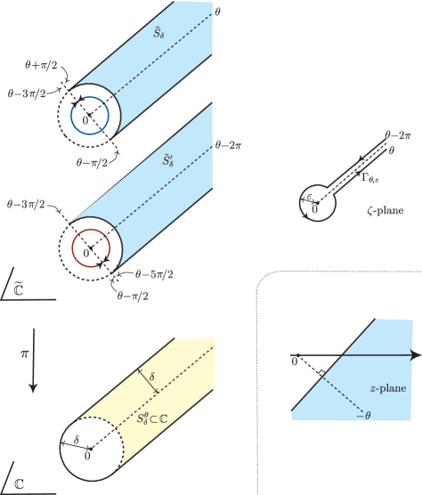
Figure 10: Laplace transform of a major. Left: the domain of $\tilde{\mathbb{C}}$ where ${\stackrel{{\scriptstyle\raisebox{-0.62386pt}{$\scriptscriptstyle\vee$}}}{{\varphi}}}$ must be holomorphic and its projection $S_{\delta}^{\theta}$ in $\mathbb{C}$. Right: the contour ${\Gamma}_{{\theta},{\varepsilon}}$ for ${\zeta}$ (above) and the domain where $z$ belongs (below).

The right-hand side of (128) is the “Laplace transform of majors”. It shows why the notation $\raisebox{-0.99025pt}{${\stackrel{{\scriptstyle\raisebox{-0.69318pt}{$\scriptscriptstyle\triangledown$}}}{{\varphi}}}$}=c\,\delta+\raisebox{-0.99025pt}{${\stackrel{{\scriptstyle\raisebox{-0.54247pt}{$\scriptscriptstyle\wedge$}}}{{\varphi}}}$}$ is consistent with the notations used in the context of $1$-summability and suggests far-reaching extensions of $1$-summability theory, which however we shall not pursue in this text (the interested reader may consult [Eca81] or [Sau06, §3.2]).

Alien calculus for simple resurgent functions

27 Simple $\Omega$-resurgent functions and alien operators

We now leave aside the summability issues and come back to resurgent functions. Let $\Omega$ be a non-empty closed discrete subset of $\mathbb{C}$ (for the moment we do not require it to be stable under addition). From now on, we shall always consider $\Omega$-resurgent functions as simple singularities (taking advantage of (126) and (127)):

$$\mathbb{C}\,\delta\oplus\hat{\mathscr{R}}_{\Omega}\,\subset\,\mathbb{C}\,\delta\oplus\mathbb{C}\{{\zeta}\}\simeq\operatorname{SING}^{\mathrm{simp}},$$

where the germs of $\hat{\mathscr{R}}_{\Omega}$ are characterized by $\Omega$-continuability.

More generally, at least when $0\in\Omega$, we define the space $\operatorname{SING}_{\Omega}$ of $\Omega$-resurgent singularities as the space of all $\raisebox{-0.99025pt}{${\stackrel{{\scriptstyle\raisebox{-0.69318pt}{$\scriptscriptstyle\triangledown$}}}{{\varphi}}}$}\in\operatorname{SING}$ whose minors $\raisebox{-0.99025pt}{${\stackrel{{\scriptstyle\raisebox{-0.54247pt}{$\scriptscriptstyle\wedge$}}}{{\varphi}}}$}=\operatorname{var}\raisebox{-0.99025pt}{${\stackrel{{\scriptstyle\raisebox{-0.69318pt}{$\scriptscriptstyle\triangledown$}}}{{\varphi}}}$}\in\operatorname{ANA}$ are $\Omega$-continuable in the following sense: denoting by $\mathcal{V}(h)\subset\tilde{\mathbb{C}}$ a domain where ${\stackrel{{\scriptstyle\raisebox{-0.54247pt}{$\scriptscriptstyle\wedge$}}}{{\varphi}}}$ defines a holomorphic function, ${\stackrel{{\scriptstyle\raisebox{-0.54247pt}{$\scriptscriptstyle\wedge$}}}{{\varphi}}}$ admits analytic continuation along any path $\tilde{\gamma}$ of $\tilde{\mathbb{C}}$ starting in $\mathcal{V}(h)$ such that $\pi\circ\tilde{\gamma}$ is contained in $\mathbb{C}\setminus\Omega$. We then have the following diagram:

Figure 11: The alien operator $\operatorname{\mathcal{A}}^{\gamma,\xi}_{\omega}$ measures the singularity at $\omega$ for the analytic continuation along $\gamma$ of an $\Omega$-continuable germ.

Definition 27.1.

Suppose that $\omega\in\Omega$, $\gamma$ is a path of $\mathbb{C}\setminus\Omega$ starting at a point ${\zeta}_{0}\in\mathbb{D}^{*}_{\rho(\Omega)}$ and ending at a point ${\zeta}_{1}$ such that there exists an open disc $D\subset\mathbb{C}\setminus\Omega$ centred at ${\zeta}_{1}$ to which $\omega$ is adherent, and $\xi\in\tilde{\mathbb{C}}$ satisfies $\pi(\xi)=-\omega+{\zeta}_{1}$. We then define a linear map, called the alien operator associated with $(\omega,\gamma,\xi)$,

$$\operatorname{\mathcal{A}}^{\gamma,\xi}_{\omega}\colon\thinspace\mathbb{C}\,\delta\oplus\hat{\mathscr{R}}_{\Omega}\to\operatorname{SING}$$

by the formula

$$\operatorname{\mathcal{A}}^{\gamma,\xi}_{\omega}(a\,\delta+\raisebox{-0.99025pt}{${\stackrel{{\scriptstyle\raisebox{-0.54247pt}{$\scriptscriptstyle\wedge$}}}{{\varphi}}}$})\coloneqq\operatorname{sing}_{0}\big{(}{\stackrel{{\scriptstyle\raisebox{-0.69318pt}{$\scriptscriptstyle\vee$}}}{{f}}}({\zeta})\big{)},\qquad{\stackrel{{\scriptstyle\raisebox{-0.69318pt}{$\scriptscriptstyle\vee$}}}{{f}}}({\zeta})=\operatorname{cont}_{\gamma}\raisebox{-0.99025pt}{${\stackrel{{\scriptstyle\raisebox{-0.54247pt}{$\scriptscriptstyle\wedge$}}}{{\varphi}}}$}\big{(}\omega+\pi({\zeta})\big{)}\enspace\text{for ${\zeta}\in\tilde{D}(\xi)$},$$ (129)

where $\tilde{D}(\xi)\subset\tilde{\mathbb{C}}$ is the connected component of $\pi^{-1}(-\omega+D)$ which contains $\xi$. See Figure 11.

This means that we follow the analytic continuation of ${\stackrel{{\scriptstyle\raisebox{-0.54247pt}{$\scriptscriptstyle\wedge$}}}{{\varphi}}}$ along $\gamma$ and get a function $\operatorname{cont}_{\gamma}\raisebox{-0.99025pt}{${\stackrel{{\scriptstyle\raisebox{-0.54247pt}{$\scriptscriptstyle\wedge$}}}{{\varphi}}}$}$ which is holomorphic in the disc $D$ centred at ${\zeta}_{1}$, of which $\omega\in\partial D$ is possibly a singular point; we then translate this picture and get a function

$${\zeta}\mapsto f({\zeta})\coloneqq\operatorname{cont}_{\gamma}\raisebox{-0.99025pt}{${\stackrel{{\scriptstyle\raisebox{-0.54247pt}{$\scriptscriptstyle\wedge$}}}{{\varphi}}}$}(\omega+{\zeta})$$

which is holomorphic in the disc $-\omega+D$ centred at $-\omega+{\zeta}_{1}=\pi(\xi)$, of which $0\in\partial(-\omega+D)$ is possibly a singular point; the function $f$ has spiral continuation around $0$ because ${\stackrel{{\scriptstyle\raisebox{-0.54247pt}{$\scriptscriptstyle\wedge$}}}{{\varphi}}}$ is $\Omega$-continuable: choosing ${\varepsilon}>0$ small enough so that $D(\omega,{\varepsilon})\cap\Omega=\{\omega\}$ (which is possible since $\Omega$ is discrete), we see that $\operatorname{cont}_{\gamma}\raisebox{-0.99025pt}{${\stackrel{{\scriptstyle\raisebox{-0.54247pt}{$\scriptscriptstyle\wedge$}}}{{\varphi}}}$}$ can be continued analytically along any path starting from ${\zeta}_{1}$ and staying in $D(\omega,{\varepsilon})\cup D$, hence ${\stackrel{{\scriptstyle\raisebox{-0.69318pt}{$\scriptscriptstyle\vee$}}}{{f}}}$ is holomorphic in $\mathcal{V}(h)\cup\tilde{D}$ with $h({\theta})\equiv{\varepsilon}$ and formula (129) makes sense.

Remark 27.2.

It is clear that the operator $\operatorname{\mathcal{A}}^{\gamma,\xi}_{\omega}$ does not change if $\gamma$ is replaced with a path which is homotopic (in $\mathbb{C}\setminus\Omega$, with fixed endpoints) to $\gamma$, nor if the endpoints of $\gamma$ are modified in a continuous way (keeping satisfied the assumptions of Definition 27.1) provided that $\xi$ is modified accordingly. On the other hand, modifying $\xi$ while keeping $\gamma$ unchanged results in an elementary modification of the result, in line with footnote 9 on p. 9.

In a nutshell, the idea is to measure the singularity at $\omega$ for the analytic continuation along $\gamma$ of the minor ${\stackrel{{\scriptstyle\raisebox{-0.54247pt}{$\scriptscriptstyle\wedge$}}}{{\varphi}}}$. Of course, if $\omega$ is not a singular point for $\operatorname{cont}_{\gamma}\raisebox{-0.99025pt}{${\stackrel{{\scriptstyle\raisebox{-0.54247pt}{$\scriptscriptstyle\wedge$}}}{{\varphi}}}$}$, then $\operatorname{\mathcal{A}}^{\gamma,\xi}_{\omega}\raisebox{-0.99025pt}{${\stackrel{{\scriptstyle\raisebox{-0.69318pt}{$\scriptscriptstyle\triangledown$}}}{{\varphi}}}$}=0$. In fact, the intersection of the kernels of all the operators $\operatorname{\mathcal{A}}^{\gamma,\xi}_{\omega}$ is $\mathbb{C}\,\delta\oplus\mathscr{O}(\mathbb{C})$, where $\mathscr{O}(\mathbb{C})$ is the set of all entire functions. In particular,

$$\mathcal{B}^{-1}\raisebox{-0.99025pt}{${\stackrel{{\scriptstyle\raisebox{-0.69318pt}{$\scriptscriptstyle\triangledown$}}}{{\varphi}}}$}\in\mathbb{C}\{z^{-1}\}\quad\Longrightarrow\quad\operatorname{\mathcal{A}}^{\gamma,\xi}_{\omega}\raisebox{-0.99025pt}{${\stackrel{{\scriptstyle\raisebox{-0.69318pt}{$\scriptscriptstyle\triangledown$}}}{{\varphi}}}$}=0.$$

Example 27.1.

We had $\raisebox{-0.99025pt}{${\stackrel{{\scriptstyle\raisebox{-0.54247pt}{$\scriptscriptstyle\wedge$}}}{{\varphi}}}$}_{\alpha}({\zeta})\coloneqq(1+{\zeta})^{\alpha-1}$ with $\alpha\in\mathbb{C}$ in Example 18.8, in connection with the incomplete Gamma function. Here we can take any $\Omega$ containing $-1$ and we have $\operatorname{\mathcal{A}}^{\gamma,\xi}_{\omega}\raisebox{-0.99025pt}{${\stackrel{{\scriptstyle\raisebox{-0.54247pt}{$\scriptscriptstyle\wedge$}}}{{\varphi}}}$}_{\alpha}=0$ whenever $\omega\neq-1$, since $-1$ is the only possible singular point of a branch of the analytic continuation of ${\stackrel{{\scriptstyle\raisebox{-0.54247pt}{$\scriptscriptstyle\wedge$}}}{{\varphi}}}$. For $\omega=-1$, the value of $\operatorname{\mathcal{A}}^{\gamma,\xi}_{-1}\raisebox{-0.99025pt}{${\stackrel{{\scriptstyle\raisebox{-0.54247pt}{$\scriptscriptstyle\wedge$}}}{{\varphi}}}$}_{\alpha}$ depends on $\gamma$ and $\xi$. If $\gamma$ is contained in the interval $(-1,0)$, then we find $f({\zeta})=\raisebox{-0.99025pt}{${\stackrel{{\scriptstyle\raisebox{-0.54247pt}{$\scriptscriptstyle\wedge$}}}{{\varphi}}}$}_{\alpha}(-1+{\zeta})=$ the principal branch of ${\zeta}^{\alpha-1}$ and, if we choose $\xi$ in the principal sheet of $\tilde{\mathbb{C}}$, then

$$\operatorname{\mathcal{A}}^{\gamma,\xi}_{-1}\raisebox{-0.99025pt}{${\stackrel{{\scriptstyle\raisebox{-0.54247pt}{$\scriptscriptstyle\wedge$}}}{{\varphi}}}$}_{\alpha}=(1-\mathrm{e}^{-2\pi{\mathrm{i}}\alpha}){\Gamma}(\alpha)\raisebox{0.86108pt}{${\stackrel{{\scriptstyle\raisebox{-0.60275pt}{$\scriptscriptstyle\triangledown$}}}{{I}}}$}_{\alpha},$$

which is $0$ if and only if $\alpha\in\mathbb{N}^{*}$ (cf. (121)). If $\gamma$ turns $N$ times around $-1$, keeping the same endpoints for $\gamma$ and the same $\xi$, then this result is multiplied by $\mathrm{e}^{2\pi{\mathrm{i}}N\alpha}$; if we multiply $\xi$ by ${\underline{\mathrm{e}}}^{2\pi{\mathrm{i}}m}$, then the result is multiplied by $\mathrm{e}^{-2\pi{\mathrm{i}}m\alpha}$. (In both cases the result is unchanged if $\alpha\in\mathbb{Z}$.)

Example 27.2.

Let $\raisebox{-0.99025pt}{${\stackrel{{\scriptstyle\raisebox{-0.54247pt}{$\scriptscriptstyle\wedge$}}}{{\varphi}}}$}({\zeta})=\frac{1}{{\zeta}}\mathrm{Log\hskip 1.5pt}(1+{\zeta})$ (variant of Example 18.5) and $\Omega=\{-1,0\}$; we shall describe the logarithmic singularity which arises at $-1$ and the simple pole at $0$ for every branch of the analytic continuation of ${\stackrel{{\scriptstyle\raisebox{-0.54247pt}{$\scriptscriptstyle\wedge$}}}{{\varphi}}}$. Consider first a path $\gamma$ contained in the interval $(-1,0)$ and ending at ${\zeta}_{1}=-\tfrac{1}{2}$. For any $\xi$ projecting onto $0+{\zeta}_{1}=-\tfrac{1}{2}$, we find $\operatorname{\mathcal{A}}^{\gamma,\xi}_{0}\raisebox{-0.99025pt}{${\stackrel{{\scriptstyle\raisebox{-0.54247pt}{$\scriptscriptstyle\wedge$}}}{{\varphi}}}$}=0$ (no singularity at the origin for the principal branch), while for $\xi$ projecting onto $1+{\zeta}_{1}=\tfrac{1}{2}$,

$$\xi=\tfrac{1}{2}\,{\underline{\mathrm{e}}}^{2\pi{\mathrm{i}}m}\quad\Longrightarrow\quad\operatorname{\mathcal{A}}^{\gamma,\xi}_{-1}\raisebox{-0.99025pt}{${\stackrel{{\scriptstyle\raisebox{-0.54247pt}{$\scriptscriptstyle\wedge$}}}{{\varphi}}}$}=\operatorname{sing}_{0}\Big{(}\frac{1}{-1+{\zeta}}(-2\pi{\mathrm{i}}m+\log{\zeta})\Big{)}=-\frac{2\pi{\mathrm{i}}}{1-{\zeta}}$$

(using the notation (127)). If $\gamma$ turns $N$ times around $-1$, then the analytic continuation of ${\stackrel{{\scriptstyle\raisebox{-0.54247pt}{$\scriptscriptstyle\wedge$}}}{{\varphi}}}$ is augmented by $\frac{2\pi{\mathrm{i}}N}{{\zeta}}$, which is regular at $-1$ but singular at $0$, hence $\operatorname{\mathcal{A}}^{\gamma,\xi}_{-1}\raisebox{-0.99025pt}{${\stackrel{{\scriptstyle\raisebox{-0.54247pt}{$\scriptscriptstyle\wedge$}}}{{\varphi}}}$}$ still coincides with $-\frac{2\pi{\mathrm{i}}}{1-{\zeta}}$ (the logarithmic singularity at $-1$ is the same for every branch) but

$$\xi=-\tfrac{1}{2}\,{\underline{\mathrm{e}}}^{2\pi{\mathrm{i}}m}\quad\Longrightarrow\quad\operatorname{\mathcal{A}}^{\gamma,\xi}_{0}\raisebox{-0.99025pt}{${\stackrel{{\scriptstyle\raisebox{-0.54247pt}{$\scriptscriptstyle\wedge$}}}{{\varphi}}}$}=\operatorname{sing}_{0}\Big{(}\frac{2\pi{\mathrm{i}}N}{{\zeta}}\Big{)}=(2\pi{\mathrm{i}})^{2}N\delta.$$

Exercise 27.3.

Consider $\raisebox{-0.99025pt}{${\stackrel{{\scriptstyle\raisebox{-0.54247pt}{$\scriptscriptstyle\wedge$}}}{{\varphi}}}$}({\zeta})=-\frac{1}{{\zeta}}\mathrm{Log\hskip 1.5pt}(1-{\zeta})$ as in Example 18.5, with $\Omega=\{0,1\}$, and a path $\gamma$ contained in $(0,1)$ and ending at ${\zeta}_{1}=\tfrac{1}{2}$. Prove that $\operatorname{\mathcal{A}}^{\gamma,\xi}_{1}\raisebox{-0.99025pt}{${\stackrel{{\scriptstyle\raisebox{-0.54247pt}{$\scriptscriptstyle\wedge$}}}{{\varphi}}}$}=-\frac{2\pi{\mathrm{i}}}{1+{\zeta}}$ for any $\xi$ projecting onto $-1+{\zeta}_{1}=-\tfrac{1}{2}$. Compute $\operatorname{\mathcal{A}}^{\gamma,\xi}_{0}\raisebox{-0.99025pt}{${\stackrel{{\scriptstyle\raisebox{-0.54247pt}{$\scriptscriptstyle\wedge$}}}{{\varphi}}}$}$ for $\gamma$ turning $N$ times around $1$ and $\xi$ projecting onto $0+{\zeta}_{1}=\tfrac{1}{2}$.

Examples 18.5 and 27.2 (but not Example 18.8 if $\alpha\notin\mathbb{N}$) are particular cases of

Definition 27.3.

We call simple $\Omega$-resurgent function any $\Omega$-resurgent function ${\stackrel{{\scriptstyle\raisebox{-0.69318pt}{$\scriptscriptstyle\triangledown$}}}{{\varphi}}}$ such that, for all $(\omega,\gamma,\xi)$ as in Definition 27.1, $\operatorname{\mathcal{A}}^{\gamma,\xi}_{\omega}\raisebox{-0.99025pt}{${\stackrel{{\scriptstyle\raisebox{-0.69318pt}{$\scriptscriptstyle\triangledown$}}}{{\varphi}}}$}$ is a simple singularity. The set of all simple $\Omega$-resurgent functions is denoted by

$$\mathbb{C}\,\delta\oplus\hat{\mathscr{R}}_{\Omega}^{\mathrm{simp}},$$

where $\hat{\mathscr{R}}_{\Omega}^{\mathrm{simp}}$ is the set of all simple $\Omega$-resurgent functions without constant term. We call simple $\Omega$-resurgent series any element of

$$\tilde{\mathscr{R}}_{\Omega}^{\mathrm{simp}}\coloneqq\mathcal{B}^{-1}\big{(}\mathbb{C}\,\delta\oplus\hat{\mathscr{R}}_{\Omega}^{\mathrm{simp}}\big{)}\subset\tilde{\mathscr{R}}_{\Omega}.$$

Lemma 27.4.

Let $\omega,\gamma,\xi$ be as in Definition 27.1. Then

$$\raisebox{-0.99025pt}{${\stackrel{{\scriptstyle\raisebox{-0.69318pt}{$\scriptscriptstyle\triangledown$}}}{{\varphi}}}$}\in\mathbb{C}\,\delta\oplus\hat{\mathscr{R}}_{\Omega}\quad \Longrightarrow\quad\operatorname{\mathcal{A}}^{\gamma,\xi}_{\omega}\raisebox{-0.99025pt}{${\stackrel{{\scriptstyle\raisebox{-0.69318pt}{$\scriptscriptstyle\triangledown$}}}{{\varphi}}}$}\in\operatorname{SING}_{-\omega+\Omega}$$

$$\raisebox{-0.99025pt}{${\stackrel{{\scriptstyle\raisebox{-0.69318pt}{$\scriptscriptstyle\triangledown$}}}{{\varphi}}}$}\in\mathbb{C}\,\delta\oplus\hat{\mathscr{R}}_{\Omega}^{\mathrm{simp}}\quad \Longrightarrow\quad\operatorname{\mathcal{A}}^{\gamma,\xi}_{\omega}\raisebox{-0.99025pt}{${\stackrel{{\scriptstyle\raisebox{-0.69318pt}{$\scriptscriptstyle\triangledown$}}}{{\varphi}}}$}\in\mathbb{C}\,\delta\oplus\hat{\mathscr{R}}_{-\omega+\Omega}^{\mathrm{simp}}.$$

Moreover, in the last case, $\operatorname{\mathcal{A}}^{\gamma,\xi}_{\omega}\raisebox{-0.99025pt}{${\stackrel{{\scriptstyle\raisebox{-0.69318pt}{$\scriptscriptstyle\triangledown$}}}{{\varphi}}}$}$ does not depend on the choice of $\xi$ in $\pi^{-1}(-\omega+{\zeta}_{1})$; denoting it by $\operatorname{\mathcal{A}}^{\gamma}_{\omega}\raisebox{-0.99025pt}{${\stackrel{{\scriptstyle\raisebox{-0.69318pt}{$\scriptscriptstyle\triangledown$}}}{{\varphi}}}$}$, we thus define an operator $\operatorname{\mathcal{A}}^{\gamma}_{\omega}\colon\thinspace\mathbb{C}\,\delta\oplus\hat{\mathscr{R}}_{\Omega}^{\mathrm{simp}}\to\mathbb{C}\,\delta\oplus\hat{\mathscr{R}}_{-\omega+\Omega}^{\mathrm{simp}}$.

Proof of Lemma 27.4.

Let $\raisebox{-0.99025pt}{${\stackrel{{\scriptstyle\raisebox{-0.69318pt}{$\scriptscriptstyle\triangledown$}}}{{\varphi}}}$}\in\mathbb{C}\,\delta\oplus\hat{\mathscr{R}}_{\Omega}$ and ${\stackrel{{\scriptstyle\raisebox{-0.69318pt}{$\scriptscriptstyle\triangledown$}}}{{\psi}}}\coloneqq\operatorname{\mathcal{A}}^{\gamma,\xi}_{\omega}\raisebox{-0.99025pt}{${\stackrel{{\scriptstyle\raisebox{-0.69318pt}{$\scriptscriptstyle\triangledown$}}}{{\varphi}}}$}\in\operatorname{SING}$, ${\stackrel{{\scriptstyle\raisebox{-0.69318pt}{$\scriptscriptstyle\wedge$}}}{{\psi}}}\coloneqq\operatorname{var}{\stackrel{{\scriptstyle\raisebox{-0.69318pt}{$\scriptscriptstyle\triangledown$}}}{{\psi}}}\in\operatorname{ANA}$. With the notations of Definition 27.1 and ${\varepsilon}$ as in the paragraph which follows it, we consider the path $\gamma^{\prime}$ obtained by concatenating $\gamma$ and a loop of $D(\omega,{\varepsilon})\cup D$ that starts and ends at ${\zeta}_{1}$ and encircles $\omega$ clockwise. We then have ${\stackrel{{\scriptstyle\raisebox{-0.69318pt}{$\scriptscriptstyle\wedge$}}}{{\psi}}}={\stackrel{{\scriptstyle\raisebox{-0.69318pt}{$\scriptscriptstyle\vee$}}}{{f}}}-{\stackrel{{\scriptstyle\raisebox{-0.69318pt}{$\scriptscriptstyle\vee$}}}{{g}}}$, with

$${\stackrel{{\scriptstyle\raisebox{-0.69318pt}{$\scriptscriptstyle\vee$}}}{{f}}}({\zeta})\coloneqq\operatorname{cont}_{\gamma}\raisebox{-0.99025pt}{${\stackrel{{\scriptstyle\raisebox{-0.54247pt}{$\scriptscriptstyle\wedge$}}}{{\varphi}}}$}\big{(}\omega+\pi({\zeta})\big{)}\quad\text{and}\quad\raisebox{-1.3347pt}{${\stackrel{{\scriptstyle\raisebox{-0.69318pt}{$\scriptscriptstyle\vee$}}}{{g}}}$}({\zeta})\coloneqq\operatorname{cont}_{\gamma^{\prime}}\raisebox{-0.99025pt}{${\stackrel{{\scriptstyle\raisebox{-0.54247pt}{$\scriptscriptstyle\wedge$}}}{{\varphi}}}$}\big{(}\omega+\pi({\zeta})\big{)}\quad\text{for ${\zeta}\in\tilde{D}$},$$

where $\tilde{D}$ is the connected component of $\pi^{-1}(D)$ which contains $\xi$.

For any path $\tilde{\lambda}$ of $\tilde{\mathbb{C}}$ which starts at $\xi$ and whose projection $\lambda\coloneqq\pi\circ\tilde{\lambda}$ is contained in $\mathbb{C}\setminus(-\omega+\Omega)$, the analytic continuation of ${\stackrel{{\scriptstyle\raisebox{-0.69318pt}{$\scriptscriptstyle\vee$}}}{{f}}}$ and ${\stackrel{{\scriptstyle\raisebox{-0.69318pt}{$\scriptscriptstyle\vee$}}}{{g}}}$ along $\tilde{\lambda}$ exists and is given by

$$\operatorname{cont}_{\tilde{\lambda}}{\stackrel{{\scriptstyle\raisebox{-0.69318pt}{$\scriptscriptstyle\vee$}}}{{f}}}({\zeta})=\operatorname{cont}_{\Gamma}\raisebox{-0.99025pt}{${\stackrel{{\scriptstyle\raisebox{-0.54247pt}{$\scriptscriptstyle\wedge$}}}{{\varphi}}}$}\big{(}\omega+\pi({\zeta})\big{)},\qquad\operatorname{cont}_{\tilde{\lambda}}\raisebox{-1.3347pt}{${\stackrel{{\scriptstyle\raisebox{-0.69318pt}{$\scriptscriptstyle\vee$}}}{{g}}}$}({\zeta})=\operatorname{cont}_{{\Gamma}^{\prime}}\raisebox{-0.99025pt}{${\stackrel{{\scriptstyle\raisebox{-0.54247pt}{$\scriptscriptstyle\wedge$}}}{{\varphi}}}$}\big{(}\omega+\pi({\zeta})\big{)},$$

where ${\Gamma}$ is obtained by concatenating $\gamma$ and $\omega+\lambda$, and ${\Gamma}^{\prime}$ by concatenating $\gamma^{\prime}$ and $\omega+\lambda$. Hence the analytic continuation of ${\stackrel{{\scriptstyle\raisebox{-0.69318pt}{$\scriptscriptstyle\wedge$}}}{{\psi}}}$ along any such path $\tilde{\lambda}$ exists, and this is sufficient to ensure that ${\stackrel{{\scriptstyle\raisebox{-0.69318pt}{$\scriptscriptstyle\triangledown$}}}{{\psi}}}\in\operatorname{SING}_{\Omega}$, which was the first statement to be proved.

If we suppose $\raisebox{-0.99025pt}{${\stackrel{{\scriptstyle\raisebox{-0.69318pt}{$\scriptscriptstyle\triangledown$}}}{{\varphi}}}$}\in\mathbb{C}\,\delta\oplus\hat{\mathscr{R}}_{\Omega}^{\mathrm{simp}}$, then $\raisebox{-0.99025pt}{${\stackrel{{\scriptstyle\raisebox{-0.69318pt}{$\scriptscriptstyle\triangledown$}}}{{\psi}}}$}\in\operatorname{SING}^{\mathrm{simp}}$, and the second statement follows from Example 25.1 and Remark 25.4: changing $\xi$ amounts to adding to ${\stackrel{{\scriptstyle\raisebox{-0.69318pt}{$\scriptscriptstyle\vee$}}}{{f}}}$ an integer multiple of ${\stackrel{{\scriptstyle\raisebox{-0.69318pt}{$\scriptscriptstyle\wedge$}}}{{\psi}}}$ which is now assumed to be regular at the origin, and hence does not modify $\operatorname{sing}_{0}\big{(}{\stackrel{{\scriptstyle\raisebox{-0.69318pt}{$\scriptscriptstyle\vee$}}}{{f}}}({\zeta})\big{)}$. Putting these facts together, we obtain $\operatorname{\mathcal{A}}^{\gamma,\xi}_{\omega}\raisebox{-0.99025pt}{${\stackrel{{\scriptstyle\raisebox{-0.69318pt}{$\scriptscriptstyle\triangledown$}}}{{\varphi}}}$}\in\operatorname{SING}_{-\omega+\Omega}\cap\operatorname{SING}^{\mathrm{simp}}=\mathbb{C}\,\delta\oplus\hat{\mathscr{R}}_{-\omega+\Omega}^{\mathrm{simp}}$ independent of $\xi$. ∎

In other words, an $\Omega$-resurgent function ${\stackrel{{\scriptstyle\raisebox{-0.69318pt}{$\scriptscriptstyle\triangledown$}}}{{\varphi}}}$ is simple if and only if all the branches of the analytic continuation of the minor $\raisebox{-0.99025pt}{${\stackrel{{\scriptstyle\raisebox{-0.54247pt}{$\scriptscriptstyle\wedge$}}}{{\varphi}}}$}=\operatorname{var}\raisebox{-0.99025pt}{${\stackrel{{\scriptstyle\raisebox{-0.69318pt}{$\scriptscriptstyle\triangledown$}}}{{\varphi}}}$}$ have only simple singularities; the relation $\operatorname{\mathcal{A}}^{\gamma}_{\omega}\raisebox{-0.99025pt}{${\stackrel{{\scriptstyle\raisebox{-0.69318pt}{$\scriptscriptstyle\triangledown$}}}{{\varphi}}}$}=a\,\delta+{\stackrel{{\scriptstyle\raisebox{-0.69318pt}{$\scriptscriptstyle\wedge$}}}{{\psi}}}({\zeta})$ then means

$$\operatorname{cont}_{\gamma}\raisebox{-0.99025pt}{${\stackrel{{\scriptstyle\raisebox{-0.54247pt}{$\scriptscriptstyle\wedge$}}}{{\varphi}}}$}(\omega+{\zeta})=\frac{a}{2\pi{\mathrm{i}}{\zeta}}+{\stackrel{{\scriptstyle\raisebox{-0.69318pt}{$\scriptscriptstyle\wedge$}}}{{\psi}}}({\zeta})\frac{\mathrm{\mathscr{L}og\hskip 1.5pt}{\zeta}}{2\pi{\mathrm{i}}}+R({\zeta})$$ (130)

for ${\zeta}$ close enough to $0$, where $\mathrm{\mathscr{L}og\hskip 1.5pt}{\zeta}$ is any branch of the logarithm and $R({\zeta})\in\mathbb{C}\{{\zeta}\}$.

Notation 27.5.

We just defined an operator $\operatorname{\mathcal{A}}^{\gamma}_{\omega}\colon\thinspace\mathbb{C}\,\delta\oplus\hat{\mathscr{R}}_{\Omega}^{\mathrm{simp}}\to\mathbb{C}\,\delta\oplus\hat{\mathscr{R}}_{-\omega+\Omega}^{\mathrm{simp}}$. We shall denote by the same symbol the counterpart of this operator in spaces of formal series:

Definition 27.6.

Let $\omega\in\Omega$. We call alien operator at $\omega$ any linear combination of composite operators of the form

$$\operatorname{\mathcal{A}}^{\gamma_{r}}_{\omega-\omega_{r-1}}\circ\cdots\circ\operatorname{\mathcal{A}}^{\gamma_{2}}_{\omega_{2}-\omega_{1}}\circ\operatorname{\mathcal{A}}^{\gamma_{1}}_{\omega_{1}}$$

(viewed as operators $\mathbb{C}\,\delta\oplus\hat{\mathscr{R}}_{\Omega}^{\mathrm{simp}}\to\mathbb{C}\,\delta\oplus\hat{\mathscr{R}}_{-\omega+\Omega}^{\mathrm{simp}}$ or, equivalently, $\tilde{\mathscr{R}}_{\Omega}^{\mathrm{simp}}\to\tilde{\mathscr{R}}_{-\omega+\Omega}^{\mathrm{simp}}$) with any $r\geq 1$, $\omega_{1},\ldots,\omega_{r-1}\in\Omega$, $\gamma_{j}$ being any path of $\mathbb{C}\setminus(-\omega_{j-1}+\Omega)$ starting in $\mathbb{D}^{*}_{\rho(-\omega_{j-1}+\Omega)}$ and ending in a disc $D_{j}\subset\mathbb{D}\setminus(-\omega_{j-1}+\Omega)$ to which $\omega_{j}-\omega_{j-1}$ is adherent, with the conventions $\omega_{0}=0$ and $\omega_{r}=\omega$, so that $\operatorname{\mathcal{A}}^{\gamma_{j}}_{\omega_{j}-\omega_{j-1}}\colon\thinspace\tilde{\mathscr{R}}_{-\omega_{j-1}+\Omega}^{\mathrm{simp}}\to\tilde{\mathscr{R}}_{-\omega_{j}+\Omega}^{\mathrm{simp}}$ is well defined.

Clearly $\mathbb{C}\,\delta\oplus\mathscr{O}(\mathbb{C})\subset\mathbb{C}\,\delta\oplus\hat{\mathscr{R}}_{\Omega}^{\mathrm{simp}}$ (since an entire function has no singularity at all!), hence

$$\mathbb{C}\{z^{-1}\}\subset\tilde{\mathscr{R}}_{\Omega}^{\mathrm{simp}},$$

and of course all alien operators act trivially on such resurgent functions. Another easy example of simple $\Omega$-resurgent function is provided by any meromorphic function ${\stackrel{{\scriptstyle\raisebox{-0.54247pt}{$\scriptscriptstyle\wedge$}}}{{\varphi}}}$ of ${\zeta}$ which is regular at $0$ and whose poles are all simple and located in $\Omega$. In this case $\operatorname{\mathcal{A}}^{\gamma}_{\omega}\raisebox{-0.99025pt}{${\stackrel{{\scriptstyle\raisebox{-0.54247pt}{$\scriptscriptstyle\wedge$}}}{{\varphi}}}$}$ does not depend on $\gamma$: its value is $2\pi{\mathrm{i}}c_{\omega}\delta$, where $c_{\omega}$ is the residuum of ${\stackrel{{\scriptstyle\raisebox{-0.54247pt}{$\scriptscriptstyle\wedge$}}}{{\varphi}}}$ at $\omega$.

Example 27.4.

By looking at the proof of Lemma 18.4, we see that we have meromorphic Borel transforms for the formal series associated with the names of Euler, Poincaré and Stirling, hence

$$\tilde{\varphi}^{\raisebox{-0.69318pt}{$\scriptstyle\mathrm{E}$}}\in\tilde{\mathscr{R}}_{\{-1\}}^{\mathrm{simp}},\qquad\tilde{\varphi}^{\raisebox{-0.69318pt}{$\scriptstyle\mathrm{P}$}}\in\tilde{\mathscr{R}}_{s+2\pi{\mathrm{i}}\,\mathbb{Z}}^{\mathrm{simp}},\qquad\tilde{\mu}\in\tilde{\mathscr{R}}_{2\pi{\mathrm{i}}\,\mathbb{Z}^{*}}^{\mathrm{simp}},$$

and we can compute

$$\operatorname{\mathcal{A}}^{\gamma}_{-1}\raisebox{-0.99025pt}{${\stackrel{{\scriptstyle\raisebox{-0.54247pt}{$\scriptscriptstyle\wedge$}}}{{\varphi}}}$}^{\raisebox{-2.50153pt}{$\scriptstyle\mathrm{E}$}}=2\pi{\mathrm{i}}\delta,\qquad\operatorname{\mathcal{A}}^{\gamma}_{s+2\pi{\mathrm{i}}k}\raisebox{-0.99025pt}{${\stackrel{{\scriptstyle\raisebox{-0.54247pt}{$\scriptscriptstyle\wedge$}}}{{\varphi}}}$}^{\raisebox{-2.50153pt}{$\scriptstyle\mathrm{P}$}}=2\pi{\mathrm{i}}\delta,\qquad\operatorname{\mathcal{A}}^{\gamma}_{2\pi{\mathrm{i}}m}\raisebox{-0.99025pt}{${\stackrel{{\scriptstyle\raisebox{-0.54247pt}{$\scriptscriptstyle\wedge$}}}{{\mu}}}$}=\frac{1}{m}\delta,$$

for $k\in\mathbb{Z}$, $m\in\mathbb{Z}^{*}$ with any $\gamma$ (and correspondingly $\operatorname{\mathcal{A}}^{\gamma}_{-1}\tilde{\varphi}^{\raisebox{-0.69318pt}{$\scriptstyle\mathrm{E}$}}=\operatorname{\mathcal{A}}^{\gamma}_{s+2\pi{\mathrm{i}}k}\tilde{\varphi}^{\raisebox{-0.69318pt}{$\scriptstyle\mathrm{P}$}}=2\pi{\mathrm{i}}$, $\operatorname{\mathcal{A}}^{\gamma}_{2\pi{\mathrm{i}}m}\tilde{\mu}=\frac{1}{m}$). A less elementary example is $\tilde{\lambda}=\mathrm{e}^{\tilde{\mu}}$; we saw that $\tilde{\lambda}\in\tilde{\mathscr{R}}_{2\pi{\mathrm{i}}\,\mathbb{Z}}$ in Example 22.1, we shall see in Section 30.1 that it belongs to $\tilde{\mathscr{R}}_{2\pi{\mathrm{i}}\,\mathbb{Z}}^{\mathrm{simp}}$ and that any alien operator maps $\tilde{\lambda}$ to a multiple of $\tilde{\lambda}$.

Here is a variant of Lemma 18.6 adapted to the case of simple resurgent functions:

Lemma 27.7.

Let $\Omega$ be any non-empty closed discrete subset of $\mathbb{C}$.

1. If ${\stackrel{{\scriptstyle\raisebox{-0.60275pt}{$\scriptscriptstyle\wedge$}}}{{B}}}$ is an entire function, then multiplication by ${\stackrel{{\scriptstyle\raisebox{-0.60275pt}{$\scriptscriptstyle\wedge$}}}{{B}}}$ leaves $\hat{\mathscr{R}}_{\Omega}^{\mathrm{simp}}$ invariant, with

   $$\operatorname{\mathcal{A}}^{\gamma}_{\omega}\raisebox{-0.99025pt}{${\stackrel{{\scriptstyle\raisebox{-0.54247pt}{$\scriptscriptstyle\wedge$}}}{{\varphi}}}$}=a\,\delta+{\stackrel{{\scriptstyle\raisebox{-0.69318pt}{$\scriptscriptstyle\wedge$}}}{{\psi}}}({\zeta})\enspace\Longrightarrow\enspace\operatorname{\mathcal{A}}^{\gamma}_{\omega}(\raisebox{0.86108pt}{${\stackrel{{\scriptstyle\raisebox{-0.60275pt}{$\scriptscriptstyle\wedge$}}}{{B}}}$}\raisebox{-0.99025pt}{${\stackrel{{\scriptstyle\raisebox{-0.54247pt}{$\scriptscriptstyle\wedge$}}}{{\varphi}}}$})=\raisebox{0.86108pt}{${\stackrel{{\scriptstyle\raisebox{-0.60275pt}{$\scriptscriptstyle\wedge$}}}{{B}}}$}(\omega)a\,\delta+\raisebox{0.86108pt}{${\stackrel{{\scriptstyle\raisebox{-0.60275pt}{$\scriptscriptstyle\wedge$}}}{{B}}}$}(\omega+{\zeta}){\stackrel{{\scriptstyle\raisebox{-0.69318pt}{$\scriptscriptstyle\wedge$}}}{{\psi}}}({\zeta}).$$ (131)

2. As a consequence, for any $c\in\mathbb{C}$, the operators $\hat{\partial}$ and $\hat{T}_{c}$ (defined by (21) and (23)) leave $\mathbb{C}\,\delta\oplus\hat{\mathscr{R}}_{\Omega}^{\mathrm{simp}}$ invariant or, equivalently, $\tilde{\mathscr{R}}_{\Omega}^{\mathrm{simp}}$ is stable by $\partial=\frac{{\mathrm{d}}\,}{{\mathrm{d}}z}$ and $T_{c}$; one has

   $$\tilde{\varphi}_{0}\in\tilde{\mathscr{R}}_{\Omega}^{\mathrm{simp}}\enspace\Longrightarrow\enspace\mathcal{A}_{\omega}^{\gamma}(\partial\tilde{\varphi}_{0})=(-\omega+\partial)\mathcal{A}_{\omega}^{\gamma}\tilde{\varphi}_{0}\enspace\text{and}\enspace\mathcal{A}_{\omega}^{\gamma}(T_{c}\tilde{\varphi}_{0})=\mathrm{e}^{-c\omega}T_{c}(\mathcal{A}_{\omega}^{\gamma}\tilde{\varphi}_{0}).$$ (132)

3. If $\tilde{\psi}\in z^{-2}\mathbb{C}\{z^{-1}\}$, then the solution in $z^{-1}\mathbb{C}[[z^{-1}]]$ of the difference equation

   $$\tilde{\varphi}(z+1)-\tilde{\varphi}(z)=\tilde{\psi}(z)$$

   belongs to $\tilde{\mathscr{R}}_{2\pi{\mathrm{i}}\,\mathbb{Z}^{*}}^{\mathrm{simp}}$, with $\operatorname{\mathcal{A}}^{\gamma}_{\omega}\raisebox{-0.99025pt}{${\stackrel{{\scriptstyle\raisebox{-0.54247pt}{$\scriptscriptstyle\wedge$}}}{{\varphi}}}$}=-2\pi{\mathrm{i}}{\stackrel{{\scriptstyle\raisebox{-0.69318pt}{$\scriptscriptstyle\wedge$}}}{{\psi}}}(\omega)\,\delta$ for all $(\omega,\gamma)$ with $\omega\in 2\pi{\mathrm{i}}\,\mathbb{Z}^{*}$.

Proof.

Suppose that $\operatorname{\mathcal{A}}^{\gamma}_{\omega}\raisebox{-0.99025pt}{${\stackrel{{\scriptstyle\raisebox{-0.54247pt}{$\scriptscriptstyle\wedge$}}}{{\varphi}}}$}=a\,\delta+{\stackrel{{\scriptstyle\raisebox{-0.69318pt}{$\scriptscriptstyle\wedge$}}}{{\psi}}}({\zeta})$. Since multiplication by ${\stackrel{{\scriptstyle\raisebox{-0.60275pt}{$\scriptscriptstyle\wedge$}}}{{B}}}$ commutes with analytic continuation, the relation (130) implies

$$\operatorname{cont}_{\gamma}\big{(}\raisebox{0.86108pt}{${\stackrel{{\scriptstyle\raisebox{-0.60275pt}{$\scriptscriptstyle\wedge$}}}{{B}}}$}\raisebox{-0.99025pt}{${\stackrel{{\scriptstyle\raisebox{-0.54247pt}{$\scriptscriptstyle\wedge$}}}{{\varphi}}}$}\big{)}(\omega+{\zeta})=\raisebox{0.86108pt}{${\stackrel{{\scriptstyle\raisebox{-0.60275pt}{$\scriptscriptstyle\wedge$}}}{{B}}}$}(\omega+{\zeta})\operatorname{cont}_{\gamma}\raisebox{-0.99025pt}{${\stackrel{{\scriptstyle\raisebox{-0.54247pt}{$\scriptscriptstyle\wedge$}}}{{\varphi}}}$}(\omega+{\zeta})=\frac{\raisebox{0.86108pt}{${\stackrel{{\scriptstyle\raisebox{-0.60275pt}{$\scriptscriptstyle\wedge$}}}{{B}}}$}(\omega)a}{2\pi{\mathrm{i}}{\zeta}}+\raisebox{0.86108pt}{${\stackrel{{\scriptstyle\raisebox{-0.60275pt}{$\scriptscriptstyle\wedge$}}}{{B}}}$}(\omega+{\zeta}){\stackrel{{\scriptstyle\raisebox{-0.69318pt}{$\scriptscriptstyle\wedge$}}}{{\psi}}}({\zeta})\frac{\mathrm{\mathscr{L}og\hskip 1.5pt}{\zeta}}{2\pi{\mathrm{i}}}+R^{*}({\zeta})$$

with $R^{*}({\zeta})=R({\zeta})+a\dfrac{\raisebox{0.86108pt}{${\stackrel{{\scriptstyle\raisebox{-0.60275pt}{$\scriptscriptstyle\wedge$}}}{{B}}}$}(\omega+{\zeta})-\raisebox{0.86108pt}{${\stackrel{{\scriptstyle\raisebox{-0.60275pt}{$\scriptscriptstyle\wedge$}}}{{B}}}$}(\omega)}{2\pi{\mathrm{i}}{\zeta}}\in\mathbb{C}\{{\zeta}\}$, hence $\operatorname{\mathcal{A}}^{\gamma}_{\omega}(\raisebox{0.86108pt}{${\stackrel{{\scriptstyle\raisebox{-0.60275pt}{$\scriptscriptstyle\wedge$}}}{{B}}}$}\raisebox{-0.99025pt}{${\stackrel{{\scriptstyle\raisebox{-0.54247pt}{$\scriptscriptstyle\wedge$}}}{{\varphi}}}$})=\raisebox{0.86108pt}{${\stackrel{{\scriptstyle\raisebox{-0.60275pt}{$\scriptscriptstyle\wedge$}}}{{B}}}$}(\omega)a\,\delta+\raisebox{0.86108pt}{${\stackrel{{\scriptstyle\raisebox{-0.60275pt}{$\scriptscriptstyle\wedge$}}}{{B}}}$}(\omega+{\zeta}){\stackrel{{\scriptstyle\raisebox{-0.69318pt}{$\scriptscriptstyle\wedge$}}}{{\psi}}}({\zeta})$.

Suppose now that $\tilde{\varphi}_{0}\in\tilde{\mathscr{R}}_{\Omega}^{\mathrm{simp}}$ has Borel transform $\raisebox{-0.99025pt}{${\stackrel{{\scriptstyle\raisebox{-0.69318pt}{$\scriptscriptstyle\triangledown$}}}{{\varphi}}}$}_{0}=\alpha\,\delta+\raisebox{-0.99025pt}{${\stackrel{{\scriptstyle\raisebox{-0.54247pt}{$\scriptscriptstyle\wedge$}}}{{\varphi}}}$}$ with $\alpha\in\mathbb{C}$ and ${\stackrel{{\scriptstyle\raisebox{-0.54247pt}{$\scriptscriptstyle\wedge$}}}{{\varphi}}}$ as above. According to (21) and (23), we have $\hat{\partial}\raisebox{-0.99025pt}{${\stackrel{{\scriptstyle\raisebox{-0.69318pt}{$\scriptscriptstyle\triangledown$}}}{{\varphi}}}$}_{0}=-{\zeta}\raisebox{-0.99025pt}{${\stackrel{{\scriptstyle\raisebox{-0.54247pt}{$\scriptscriptstyle\wedge$}}}{{\varphi}}}$}({\zeta})$ and $\hat{T}_{c}\raisebox{-0.99025pt}{${\stackrel{{\scriptstyle\raisebox{-0.69318pt}{$\scriptscriptstyle\triangledown$}}}{{\varphi}}}$}_{0}=\alpha\,\delta+\mathrm{e}^{-c{\zeta}}\raisebox{-0.99025pt}{${\stackrel{{\scriptstyle\raisebox{-0.54247pt}{$\scriptscriptstyle\wedge$}}}{{\varphi}}}$}({\zeta})$; we see that both of them belong to $\mathbb{C}\,\delta\oplus\hat{\mathscr{R}}_{\Omega}^{\mathrm{simp}}$ by applying the first statement with $\raisebox{0.86108pt}{${\stackrel{{\scriptstyle\raisebox{-0.60275pt}{$\scriptscriptstyle\wedge$}}}{{B}}}$}({\zeta})=-{\zeta}$ or $\mathrm{e}^{-c{\zeta}}$, and

$$\mathcal{A}_{\omega}^{\gamma}(\hat{\partial}\raisebox{-0.99025pt}{${\stackrel{{\scriptstyle\raisebox{-0.69318pt}{$\scriptscriptstyle\triangledown$}}}{{\varphi}}}$}_{0}) =-\omega a\delta+(-\omega-{\zeta}){\stackrel{{\scriptstyle\raisebox{-0.69318pt}{$\scriptscriptstyle\wedge$}}}{{\psi}}}({\zeta})=(-\omega+\hat{\partial})\mathcal{A}_{\omega}^{\gamma}\raisebox{-0.99025pt}{${\stackrel{{\scriptstyle\raisebox{-0.69318pt}{$\scriptscriptstyle\triangledown$}}}{{\varphi}}}$}_{0}$$

$$\mathcal{A}_{\omega}^{\gamma}(\hat{T}_{c}\raisebox{-0.99025pt}{${\stackrel{{\scriptstyle\raisebox{-0.69318pt}{$\scriptscriptstyle\triangledown$}}}{{\varphi}}}$}_{0}) =\mathrm{e}^{-c\omega}a\delta+\mathrm{e}^{-c(\omega+{\zeta})}{\stackrel{{\scriptstyle\raisebox{-0.69318pt}{$\scriptscriptstyle\wedge$}}}{{\psi}}}({\zeta})=\mathrm{e}^{-c\omega}\hat{T}_{c}(\mathcal{A}_{\omega}^{\gamma}\raisebox{-0.99025pt}{${\stackrel{{\scriptstyle\raisebox{-0.69318pt}{$\scriptscriptstyle\triangledown$}}}{{\varphi}}}$}_{0}),$$

which is equivalent to (132).

For the last statement, we use Corollary 4.6, according to which $\raisebox{-0.99025pt}{${\stackrel{{\scriptstyle\raisebox{-0.54247pt}{$\scriptscriptstyle\wedge$}}}{{\varphi}}}$}=\raisebox{0.86108pt}{${\stackrel{{\scriptstyle\raisebox{-0.60275pt}{$\scriptscriptstyle\wedge$}}}{{B}}}$}{\stackrel{{\scriptstyle\raisebox{-0.69318pt}{$\scriptscriptstyle\wedge$}}}{{\psi}}}$ with $\raisebox{0.86108pt}{${\stackrel{{\scriptstyle\raisebox{-0.60275pt}{$\scriptscriptstyle\wedge$}}}{{B}}}$}({\zeta})=\frac{1}{\mathrm{e}^{-{\zeta}}-1}$ and ${\stackrel{{\scriptstyle\raisebox{-0.69318pt}{$\scriptscriptstyle\wedge$}}}{{\psi}}}({\zeta})\in{\zeta}\mathscr{O}(\mathbb{C})$: the function ${\stackrel{{\scriptstyle\raisebox{-0.54247pt}{$\scriptscriptstyle\wedge$}}}{{\varphi}}}$ is meromorphic on $\mathbb{C}$ and all its poles are simple and located in $\Omega=2\pi{\mathrm{i}}\,\mathbb{Z}^{*}$, therefore it is a simple $\Omega$-resurgent function and we get the values of $\mathcal{A}_{\omega}^{\gamma}\raisebox{-0.99025pt}{${\stackrel{{\scriptstyle\raisebox{-0.69318pt}{$\scriptscriptstyle\triangledown$}}}{{\varphi}}}$}$ by computing the residues of ${\stackrel{{\scriptstyle\raisebox{-0.54247pt}{$\scriptscriptstyle\wedge$}}}{{\varphi}}}$ (cf. the paragraph just before Example 27.4). ∎

Exercise 27.5.

Given $s\in\mathbb{C}$ with $\mathop{\Re e}\nolimits s>1$, the Hurwitz zeta function is defined as

$${\zeta}(s,z)=\sum_{k=0}^{\infty}\frac{1}{(z+k)^{s}},\qquad z\in\mathbb{C}\setminus\mathbb{R}^{-}$$

(using the principal branch of $(z+k)^{s}$ for each $k$). Show that, for $s\in\mathbb{N}$ with $s\geq 2$,

$$\tilde{\varphi}^{\raisebox{-0.69318pt}{$\scriptstyle\mathrm{H}$}}_{s}(z)\coloneqq\frac{1}{(s-1)z^{s-1}}+\frac{1}{2z^{s}}+\sum_{k=1}^{\infty}\binom{s+2k-1}{s-1}\frac{B_{2k}}{(s+2k-1)z^{s+2k-1}}$$

(where the Bernoulli numbers $B_{2k}$ are defined in Exercise 11.1) is a simple $2\pi{\mathrm{i}}\,\mathbb{Z}^{*}$-resurgent formal series which is $1$-summable in the directions of $I=(-\frac{\pi}{2},\frac{\pi}{2})$, with

$${\zeta}(s,z)=(\mathscr{S}^{I}\tilde{\varphi}^{\raisebox{-0.69318pt}{$\scriptstyle\mathrm{H}$}}_{s})(z)\sim_{1}\tilde{\varphi}^{\raisebox{-0.69318pt}{$\scriptstyle\mathrm{H}$}}_{s}(z).$$

Hint: Use Lemma 27.7 and prove that ${\zeta}(s,z)$ coincides with the Laplace transform of

$$\raisebox{-0.99025pt}{${\stackrel{{\scriptstyle\raisebox{-0.54247pt}{$\scriptscriptstyle\wedge$}}}{{\varphi}}}$}^{\raisebox{-2.50153pt}{$\scriptstyle\mathrm{H}$}}_{s}({\zeta})=\frac{{\zeta}^{s-1}}{{\Gamma}(s)(1-\mathrm{e}^{-{\zeta}})}.$$ (133)

Remark 27.8.

If $s\in\mathbb{C}\setminus\mathbb{N}$ has $\mathop{\Re e}\nolimits s>1$, then (133) is not regular at the origin but still provides an example of $2\pi{\mathrm{i}}\,\mathbb{Z}$-continuable minor (in the sense of the definition given in the paragraph just before Definition 27.1). In fact, there is an extension of $1$-summability theory in which the Laplace transform of $\raisebox{-0.99025pt}{${\stackrel{{\scriptstyle\raisebox{-0.54247pt}{$\scriptscriptstyle\wedge$}}}{{\varphi}}}$}^{\raisebox{-2.50153pt}{$\scriptstyle\mathrm{H}$}}_{s}$ in the directions of $(-\frac{\pi}{2},\frac{\pi}{2})$ is still defined and coincides with ${\zeta}(s,z)$ (see [Eca81], [Sau06, §3.2]).

We end this section with a look at the action of alien operators on convolution products in the “easy case” considered in Section 19.

Theorem 27.9.

Suppose that $\raisebox{0.86108pt}{${\stackrel{{\scriptstyle\raisebox{-0.60275pt}{$\scriptscriptstyle\triangledown$}}}{{B}}}$}_{0}\in\mathbb{C}\,\delta\oplus\hat{\mathscr{R}}_{\Omega}^{\mathrm{simp}}$ with $\raisebox{0.86108pt}{${\stackrel{{\scriptstyle\raisebox{-0.60275pt}{$\scriptscriptstyle\wedge$}}}{{B}}}$}\coloneqq\operatorname{var}\raisebox{0.86108pt}{${\stackrel{{\scriptstyle\raisebox{-0.60275pt}{$\scriptscriptstyle\triangledown$}}}{{B}}}$}_{0}$ entire. Then, for any $\omega\in\Omega$, all the alien operators $\mathbb{C}\,\delta\oplus\hat{\mathscr{R}}_{\Omega}^{\mathrm{simp}}\to\mathbb{C}\,\delta\oplus\hat{\mathscr{R}}_{-\omega+\Omega}^{\mathrm{simp}}$ commute with the operator of convolution with $\raisebox{0.86108pt}{${\stackrel{{\scriptstyle\raisebox{-0.60275pt}{$\scriptscriptstyle\triangledown$}}}{{B}}}$}_{0}$.

Proof.

It suffices to show that, for any $\gamma\subset\mathbb{C}\setminus\Omega$ starting at a point ${\zeta}_{0}\in\mathbb{D}_{\rho(\Omega)}^{*}$ and ending at the centre ${\zeta}_{1}$ of a disc $D\subset\mathbb{C}\setminus\Omega$ to which $\omega$ is adherent, and for any $\raisebox{-0.99025pt}{${\stackrel{{\scriptstyle\raisebox{-0.69318pt}{$\scriptscriptstyle\triangledown$}}}{{\varphi}}}$}_{0}\in\mathbb{C}\,\delta\oplus\hat{\mathscr{R}}_{\Omega}^{\mathrm{simp}}$,

$$\operatorname{\mathcal{A}}^{\gamma}_{\omega}(\raisebox{0.86108pt}{${\stackrel{{\scriptstyle\raisebox{-0.60275pt}{$\scriptscriptstyle\triangledown$}}}{{B}}}$}_{0}*\raisebox{-0.99025pt}{${\stackrel{{\scriptstyle\raisebox{-0.69318pt}{$\scriptscriptstyle\triangledown$}}}{{\varphi}}}$}_{0})=\raisebox{0.86108pt}{${\stackrel{{\scriptstyle\raisebox{-0.60275pt}{$\scriptscriptstyle\triangledown$}}}{{B}}}$}_{0}*(\operatorname{\mathcal{A}}^{\gamma}_{\omega}\raisebox{-0.99025pt}{${\stackrel{{\scriptstyle\raisebox{-0.69318pt}{$\scriptscriptstyle\triangledown$}}}{{\varphi}}}$}_{0}).$$

We can write

$$\raisebox{0.86108pt}{${\stackrel{{\scriptstyle\raisebox{-0.60275pt}{$\scriptscriptstyle\triangledown$}}}{{B}}}$}_{0}=b\delta+\raisebox{0.86108pt}{${\stackrel{{\scriptstyle\raisebox{-0.60275pt}{$\scriptscriptstyle\wedge$}}}{{B}}}$},\quad\raisebox{-0.99025pt}{${\stackrel{{\scriptstyle\raisebox{-0.69318pt}{$\scriptscriptstyle\triangledown$}}}{{\varphi}}}$}_{0}=c\delta+\raisebox{-0.99025pt}{${\stackrel{{\scriptstyle\raisebox{-0.54247pt}{$\scriptscriptstyle\wedge$}}}{{\varphi}}}$},\quad\operatorname{\mathcal{A}}^{\gamma}_{\omega}\raisebox{-0.99025pt}{${\stackrel{{\scriptstyle\raisebox{-0.69318pt}{$\scriptscriptstyle\triangledown$}}}{{\varphi}}}$}_{0}=a\delta+{\stackrel{{\scriptstyle\raisebox{-0.69318pt}{$\scriptscriptstyle\wedge$}}}{{\psi}}}.$$

Then $\raisebox{0.86108pt}{${\stackrel{{\scriptstyle\raisebox{-0.60275pt}{$\scriptscriptstyle\triangledown$}}}{{B}}}$}_{0}*\raisebox{-0.99025pt}{${\stackrel{{\scriptstyle\raisebox{-0.69318pt}{$\scriptscriptstyle\triangledown$}}}{{\varphi}}}$}_{0}=b\raisebox{-0.99025pt}{${\stackrel{{\scriptstyle\raisebox{-0.69318pt}{$\scriptscriptstyle\triangledown$}}}{{\varphi}}}$}_{0}+c\raisebox{0.86108pt}{${\stackrel{{\scriptstyle\raisebox{-0.60275pt}{$\scriptscriptstyle\wedge$}}}{{B}}}$}+\raisebox{0.86108pt}{${\stackrel{{\scriptstyle\raisebox{-0.60275pt}{$\scriptscriptstyle\wedge$}}}{{B}}}$}*\raisebox{-0.99025pt}{${\stackrel{{\scriptstyle\raisebox{-0.54247pt}{$\scriptscriptstyle\wedge$}}}{{\varphi}}}$}$ and $\operatorname{\mathcal{A}}^{\gamma}_{\omega}(\raisebox{0.86108pt}{${\stackrel{{\scriptstyle\raisebox{-0.60275pt}{$\scriptscriptstyle\triangledown$}}}{{B}}}$}_{0}*\raisebox{-0.99025pt}{${\stackrel{{\scriptstyle\raisebox{-0.69318pt}{$\scriptscriptstyle\triangledown$}}}{{\varphi}}}$}_{0})=b\operatorname{\mathcal{A}}^{\gamma}_{\omega}\raisebox{-0.99025pt}{${\stackrel{{\scriptstyle\raisebox{-0.69318pt}{$\scriptscriptstyle\triangledown$}}}{{\varphi}}}$}_{0}+\operatorname{\mathcal{A}}^{\gamma}_{\omega}(\raisebox{0.86108pt}{${\stackrel{{\scriptstyle\raisebox{-0.60275pt}{$\scriptscriptstyle\wedge$}}}{{B}}}$}*\raisebox{-0.99025pt}{${\stackrel{{\scriptstyle\raisebox{-0.54247pt}{$\scriptscriptstyle\wedge$}}}{{\varphi}}}$})$, hence we just need to prove that $\operatorname{\mathcal{A}}^{\gamma}_{\omega}(\raisebox{0.86108pt}{${\stackrel{{\scriptstyle\raisebox{-0.60275pt}{$\scriptscriptstyle\wedge$}}}{{B}}}$}*\raisebox{-0.99025pt}{${\stackrel{{\scriptstyle\raisebox{-0.54247pt}{$\scriptscriptstyle\wedge$}}}{{\varphi}}}$})=\raisebox{0.86108pt}{${\stackrel{{\scriptstyle\raisebox{-0.60275pt}{$\scriptscriptstyle\wedge$}}}{{B}}}$}*\operatorname{\mathcal{A}}^{\gamma}_{\omega}\raisebox{-0.99025pt}{${\stackrel{{\scriptstyle\raisebox{-0.54247pt}{$\scriptscriptstyle\wedge$}}}{{\varphi}}}$}$, i.e. that

$$\operatorname{\mathcal{A}}^{\gamma}_{\omega}(\raisebox{0.86108pt}{${\stackrel{{\scriptstyle\raisebox{-0.60275pt}{$\scriptscriptstyle\wedge$}}}{{B}}}$}*\raisebox{-0.99025pt}{${\stackrel{{\scriptstyle\raisebox{-0.54247pt}{$\scriptscriptstyle\wedge$}}}{{\varphi}}}$})=a\raisebox{0.86108pt}{${\stackrel{{\scriptstyle\raisebox{-0.60275pt}{$\scriptscriptstyle\wedge$}}}{{B}}}$}+\raisebox{0.86108pt}{${\stackrel{{\scriptstyle\raisebox{-0.60275pt}{$\scriptscriptstyle\wedge$}}}{{B}}}$}*{\stackrel{{\scriptstyle\raisebox{-0.69318pt}{$\scriptscriptstyle\wedge$}}}{{\psi}}}.$$

According to Lemma 19.1, we have

$$\operatorname{cont}_{\gamma}(\raisebox{0.86108pt}{${\stackrel{{\scriptstyle\raisebox{-0.60275pt}{$\scriptscriptstyle\wedge$}}}{{B}}}$}*\raisebox{-0.99025pt}{${\stackrel{{\scriptstyle\raisebox{-0.54247pt}{$\scriptscriptstyle\wedge$}}}{{\varphi}}}$})(\omega+{\zeta})=\int_{0}^{{\zeta}_{0}}\raisebox{0.86108pt}{${\stackrel{{\scriptstyle\raisebox{-0.60275pt}{$\scriptscriptstyle\wedge$}}}{{B}}}$}(\omega+{\zeta}-\xi)\raisebox{-0.99025pt}{${\stackrel{{\scriptstyle\raisebox{-0.54247pt}{$\scriptscriptstyle\wedge$}}}{{\varphi}}}$}(\xi)\,{\mathrm{d}}\xi+\int_{\gamma}\raisebox{0.86108pt}{${\stackrel{{\scriptstyle\raisebox{-0.60275pt}{$\scriptscriptstyle\wedge$}}}{{B}}}$}(\omega+{\zeta}-\xi)\raisebox{-0.99025pt}{${\stackrel{{\scriptstyle\raisebox{-0.54247pt}{$\scriptscriptstyle\wedge$}}}{{\varphi}}}$}(\xi)\,{\mathrm{d}}\xi+\int_{{\zeta}_{1}}^{\omega+{\zeta}}\raisebox{0.86108pt}{${\stackrel{{\scriptstyle\raisebox{-0.60275pt}{$\scriptscriptstyle\wedge$}}}{{B}}}$}(\omega+{\zeta}-\xi)\raisebox{-0.99025pt}{${\stackrel{{\scriptstyle\raisebox{-0.54247pt}{$\scriptscriptstyle\wedge$}}}{{\varphi}}}$}(\xi)\,{\mathrm{d}}\xi$$

for ${\zeta}\in-\omega+D$, where it is understood that $\raisebox{-0.99025pt}{${\stackrel{{\scriptstyle\raisebox{-0.54247pt}{$\scriptscriptstyle\wedge$}}}{{\varphi}}}$}(\xi)$ represents the value at $\xi$ of the appropriate branch of the analytic continuation of ${\stackrel{{\scriptstyle\raisebox{-0.54247pt}{$\scriptscriptstyle\wedge$}}}{{\varphi}}}$ (which is $\operatorname{cont}_{\gamma}\raisebox{-0.99025pt}{${\stackrel{{\scriptstyle\raisebox{-0.54247pt}{$\scriptscriptstyle\wedge$}}}{{\varphi}}}$}$ for the third integral). The standard theorem about an integral depending holomorphically on a parameter ensures that the sum $R_{1}({\zeta})$ of the first two integrals extends to an entire function of ${\zeta}$. Let $\Delta\coloneqq-\omega+D$ (a disc to which $0$ is adherent). Performing the change of variable $\xi\to\omega+\xi$ in the third integral, we get

$$\operatorname{cont}_{\gamma}(\raisebox{0.86108pt}{${\stackrel{{\scriptstyle\raisebox{-0.60275pt}{$\scriptscriptstyle\wedge$}}}{{B}}}$}*\raisebox{-0.99025pt}{${\stackrel{{\scriptstyle\raisebox{-0.54247pt}{$\scriptscriptstyle\wedge$}}}{{\varphi}}}$})(\omega+{\zeta})=R_{1}({\zeta})+\int_{{-\omega+{\zeta}_{1}}}^{{\zeta}}\raisebox{0.86108pt}{${\stackrel{{\scriptstyle\raisebox{-0.60275pt}{$\scriptscriptstyle\wedge$}}}{{B}}}$}({\zeta}-\xi)\operatorname{cont}_{\gamma}\raisebox{-0.99025pt}{${\stackrel{{\scriptstyle\raisebox{-0.54247pt}{$\scriptscriptstyle\wedge$}}}{{\varphi}}}$}(\omega+\xi)\,{\mathrm{d}}\xi,\qquad{\zeta}\in\Delta.$$

Now, according to (130), we can write

$$\operatorname{cont}_{\gamma}\raisebox{-0.99025pt}{${\stackrel{{\scriptstyle\raisebox{-0.54247pt}{$\scriptscriptstyle\wedge$}}}{{\varphi}}}$}(\omega+\xi)=S(\xi)+R_{2}(\xi),\qquad\xi\in\Delta\cap\mathbb{D}_{\rho}^{*},$$

where $\displaystyle S(\xi)=\frac{a}{2\pi{\mathrm{i}}\xi}+{\stackrel{{\scriptstyle\raisebox{-0.69318pt}{$\scriptscriptstyle\wedge$}}}{{\psi}}}(\xi)\frac{\mathrm{\mathscr{L}og\hskip 1.5pt}\xi}{2\pi{\mathrm{i}}}$, $\mathrm{\mathscr{L}og\hskip 1.5pt}\xi$ being a branch of the logarithm holomorphic in $\Delta$, $R_{2}(\xi)\in\mathbb{C}\{\xi\}$, and $\rho>0$ is smaller than the radii of convergence of ${\stackrel{{\scriptstyle\raisebox{-0.69318pt}{$\scriptscriptstyle\wedge$}}}{{\psi}}}$ and $R_{2}$. Let us pick ${\sigma}\in\Delta\cap\mathbb{D}_{\rho}^{*}$ and set

$$R({\zeta})\coloneqq R_{1}({\zeta})+\int_{{-\omega+{\zeta}_{1}}}^{{\sigma}}\raisebox{0.86108pt}{${\stackrel{{\scriptstyle\raisebox{-0.60275pt}{$\scriptscriptstyle\wedge$}}}{{B}}}$}({\zeta}-\xi)\operatorname{cont}_{\gamma}\raisebox{-0.99025pt}{${\stackrel{{\scriptstyle\raisebox{-0.54247pt}{$\scriptscriptstyle\wedge$}}}{{\varphi}}}$}(\omega+\xi)\,{\mathrm{d}}\xi,$$

so that

$$\operatorname{cont}_{\gamma}(\raisebox{0.86108pt}{${\stackrel{{\scriptstyle\raisebox{-0.60275pt}{$\scriptscriptstyle\wedge$}}}{{B}}}$}*\raisebox{-0.99025pt}{${\stackrel{{\scriptstyle\raisebox{-0.54247pt}{$\scriptscriptstyle\wedge$}}}{{\varphi}}}$})(\omega+{\zeta})=R({\zeta})+\int_{{\sigma}}^{{\zeta}}\raisebox{0.86108pt}{${\stackrel{{\scriptstyle\raisebox{-0.60275pt}{$\scriptscriptstyle\wedge$}}}{{B}}}$}({\zeta}-\xi)\operatorname{cont}_{\gamma}\raisebox{-0.99025pt}{${\stackrel{{\scriptstyle\raisebox{-0.54247pt}{$\scriptscriptstyle\wedge$}}}{{\varphi}}}$}(\omega+\xi)\,{\mathrm{d}}\xi,\qquad{\zeta}\in\Delta.$$

We see that $R({\zeta})$ extends to an entire function of ${\zeta}$ and, for ${\zeta}\in\Delta\cap\mathbb{D}_{\rho}^{*}$, the last integral can be written

$$\int_{{\sigma}}^{{\zeta}}\raisebox{0.86108pt}{${\stackrel{{\scriptstyle\raisebox{-0.60275pt}{$\scriptscriptstyle\wedge$}}}{{B}}}$}({\zeta}-\xi)\operatorname{cont}_{\gamma}\raisebox{-0.99025pt}{${\stackrel{{\scriptstyle\raisebox{-0.54247pt}{$\scriptscriptstyle\wedge$}}}{{\varphi}}}$}(\omega+\xi)\,{\mathrm{d}}\xi=f({\zeta})+R_{3}({\zeta}),\qquad f({\zeta})\coloneqq\int_{{\sigma}}^{{\zeta}}\raisebox{0.86108pt}{${\stackrel{{\scriptstyle\raisebox{-0.60275pt}{$\scriptscriptstyle\wedge$}}}{{B}}}$}({\zeta}-\xi)S(\xi)\,{\mathrm{d}}\xi,$$

with $R_{3}({\zeta})$ defined by an integral involving $R_{2}(\xi)$ and thus extending holomorphically for ${\zeta}\in\mathbb{D}_{\rho}$. The only possibly singular term in $\operatorname{cont}_{\gamma}(\raisebox{0.86108pt}{${\stackrel{{\scriptstyle\raisebox{-0.60275pt}{$\scriptscriptstyle\wedge$}}}{{B}}}$}*\raisebox{-0.99025pt}{${\stackrel{{\scriptstyle\raisebox{-0.54247pt}{$\scriptscriptstyle\wedge$}}}{{\varphi}}}$})(\omega+{\zeta})$ is thus $f({\zeta})$, which is seen to admit analytic continuation along every path ${\Gamma}$ starting from ${\sigma}$ and contained in $\mathbb{D}_{\rho}^{*}$; indeed,

$$\operatorname{cont}_{\Gamma}f({\zeta})=\int_{\Gamma}\raisebox{0.86108pt}{${\stackrel{{\scriptstyle\raisebox{-0.60275pt}{$\scriptscriptstyle\wedge$}}}{{B}}}$}({\zeta}-\xi)S(\xi)\,{\mathrm{d}}\xi.$$ (134)

In particular, $f$ has spiral continuation around $0$. We now show that it defines a simple singularity, which is none other than $a\raisebox{0.86108pt}{${\stackrel{{\scriptstyle\raisebox{-0.60275pt}{$\scriptscriptstyle\wedge$}}}{{B}}}$}+\raisebox{0.86108pt}{${\stackrel{{\scriptstyle\raisebox{-0.60275pt}{$\scriptscriptstyle\wedge$}}}{{B}}}$}*{\stackrel{{\scriptstyle\raisebox{-0.69318pt}{$\scriptscriptstyle\wedge$}}}{{\psi}}}$.

Let us first compute the difference $g\coloneqq f^{+}-f$, where we denote by $f^{+}$ the branch of the analytic continuation of $f$ obtained by starting from $\Delta\cap\mathbb{D}_{\rho}^{*}$, turning anticlockwise around $0$ and coming back to $\Delta\cap\mathbb{D}_{\rho}^{*}$. We have

$$g({\zeta})=\int_{C_{\zeta}}\raisebox{0.86108pt}{${\stackrel{{\scriptstyle\raisebox{-0.60275pt}{$\scriptscriptstyle\wedge$}}}{{B}}}$}({\zeta}-\xi)S(\xi)\,{\mathrm{d}}\xi,\qquad{\zeta}\in\Delta\cap\mathbb{D}_{\rho}^{*},$$

where $C_{\zeta}$ is the circular path $t\in[0,2\pi]\mapsto{\zeta}\,\mathrm{e}^{{\mathrm{i}}t}$. For any ${\varepsilon}\in(0,1)$, by the Cauchy theorem,

$$g({\zeta})=\int_{{\varepsilon}{\zeta}}^{\zeta}\raisebox{0.86108pt}{${\stackrel{{\scriptstyle\raisebox{-0.60275pt}{$\scriptscriptstyle\wedge$}}}{{B}}}$}({\zeta}-\xi){\stackrel{{\scriptstyle\raisebox{-0.69318pt}{$\scriptscriptstyle\wedge$}}}{{\psi}}}(\xi)\,{\mathrm{d}}\xi+\int_{C_{{\varepsilon}{\zeta}}}\raisebox{0.86108pt}{${\stackrel{{\scriptstyle\raisebox{-0.60275pt}{$\scriptscriptstyle\wedge$}}}{{B}}}$}({\zeta}-\xi)S(\xi)\,{\mathrm{d}}\xi,$$

because $S^{+}-S={\stackrel{{\scriptstyle\raisebox{-0.69318pt}{$\scriptscriptstyle\wedge$}}}{{\psi}}}$. Keeping ${\zeta}$ fixed, we let ${\varepsilon}$ tend to $0$: the first integral clearly tends to $\raisebox{0.86108pt}{${\stackrel{{\scriptstyle\raisebox{-0.60275pt}{$\scriptscriptstyle\wedge$}}}{{B}}}$}*{\stackrel{{\scriptstyle\raisebox{-0.69318pt}{$\scriptscriptstyle\wedge$}}}{{\psi}}}({\zeta})$ and the second one can be written

$$a\int_{C_{{\varepsilon}{\zeta}}}\frac{\raisebox{0.86108pt}{${\stackrel{{\scriptstyle\raisebox{-0.60275pt}{$\scriptscriptstyle\wedge$}}}{{B}}}$}({\zeta}-\xi)}{2\pi{\mathrm{i}}\xi}\,{\mathrm{d}}\xi+\int_{C_{{\varepsilon}{\zeta}}}\raisebox{0.86108pt}{${\stackrel{{\scriptstyle\raisebox{-0.60275pt}{$\scriptscriptstyle\wedge$}}}{{B}}}$}({\zeta}-\xi){\stackrel{{\scriptstyle\raisebox{-0.69318pt}{$\scriptscriptstyle\wedge$}}}{{\psi}}}(\xi)\frac{\mathrm{\mathscr{L}og\hskip 1.5pt}\xi}{2\pi{\mathrm{i}}}\,{\mathrm{d}}\xi=\\[4.30554pt] a\raisebox{0.86108pt}{${\stackrel{{\scriptstyle\raisebox{-0.60275pt}{$\scriptscriptstyle\wedge$}}}{{B}}}$}({\zeta})+\int_{0}^{2\pi}\raisebox{0.86108pt}{${\stackrel{{\scriptstyle\raisebox{-0.60275pt}{$\scriptscriptstyle\wedge$}}}{{B}}}$}({\zeta}-{\varepsilon}{\zeta}\,\mathrm{e}^{{\mathrm{i}}t}){\stackrel{{\scriptstyle\raisebox{-0.69318pt}{$\scriptscriptstyle\wedge$}}}{{\psi}}}({\varepsilon}{\zeta}\,\mathrm{e}^{{\mathrm{i}}t})\frac{\ln{\varepsilon}+\mathrm{\mathscr{L}og\hskip 1.5pt}{\zeta}+{\mathrm{i}}t}{2\pi{\mathrm{i}}}{\mathrm{i}}{\varepsilon}{\zeta}\,\mathrm{e}^{{\mathrm{i}}t}\,{\mathrm{d}}t$$

(because the analytic continuation of $\mathrm{\mathscr{L}og\hskip 1.5pt}$ is explicitly known), which tends to $a\raisebox{0.86108pt}{${\stackrel{{\scriptstyle\raisebox{-0.60275pt}{$\scriptscriptstyle\wedge$}}}{{B}}}$}({\zeta})$ since the last integral is bounded in modulus by $C{\varepsilon}\big{(}C^{\prime}+\lvert\ln{\varepsilon}\rvert\big{)}$ with appropriate constants $C,C^{\prime}$. We thus obtain

$$g({\zeta})=a\raisebox{0.86108pt}{${\stackrel{{\scriptstyle\raisebox{-0.60275pt}{$\scriptscriptstyle\wedge$}}}{{B}}}$}({\zeta})+\raisebox{0.86108pt}{${\stackrel{{\scriptstyle\raisebox{-0.60275pt}{$\scriptscriptstyle\wedge$}}}{{B}}}$}*{\stackrel{{\scriptstyle\raisebox{-0.69318pt}{$\scriptscriptstyle\wedge$}}}{{\psi}}}({\zeta}).$$

Since this function is regular at the origin and holomorphic in $\mathbb{D}_{\rho}$, we can reformulate this result on $f^{+}-f$ by saying that the function

$${\zeta}\in\Delta\cap\mathbb{D}_{\rho}^{*}\mapsto h({\zeta})\coloneqq f({\zeta})-g({\zeta})\frac{\mathrm{\mathscr{L}og\hskip 1.5pt}{\zeta}}{2\pi{\mathrm{i}}}$$

extends analytically to a (single-valued) function holomorphic in $\mathbb{D}_{\rho}^{*}$, i.e. it can be represented by a Laurent series (117).

We conclude by showing that the above function $h$ is in fact regular at the origin. For that, it is sufficient to check that, in $\mathbb{D}_{\lvert{\sigma}\rvert}^{*}$, it is bounded by $C\big{(}C^{\prime}+\ln\frac{1}{\lvert{\zeta}\rvert}\big{)}$ with appropriate constants $C,C^{\prime}$ (indeed, this will imply ${\zeta}h({\zeta})\xrightarrow[{\zeta}\to 0]{}0$, thus the origin will be a removable singularity for $h$). Observe that every point of $\mathbb{D}_{\lvert{\sigma}\rvert}^{*}$ can be written in the form ${\zeta}={\sigma}u\,\mathrm{e}^{{\mathrm{i}}v}$ with $0<u\coloneqq{\lvert{\zeta}\rvert}/{\lvert{\sigma}\rvert}<1$ and $0\leq v<2\pi$, hence it can be reached by starting from ${\sigma}$ and following the concatenation ${\Gamma}_{\zeta}$ of the circular path $t\in[0,v]\mapsto{\sigma}\mathrm{e}^{{\mathrm{i}}t}$ and the line segment $t\in[0,1]\mapsto{\sigma}\mathrm{e}^{{\mathrm{i}}v}x(t)$ with $x(t)\coloneqq 1-t(1-u)>0$, hence

$$(\operatorname{cont}_{{\Gamma}_{\zeta}}h)({\zeta})=(\operatorname{cont}_{{\Gamma}_{\zeta}}f)({\zeta})-\frac{1}{2\pi{\mathrm{i}}}g({\zeta})(\operatorname{cont}_{{\Gamma}_{\zeta}}\mathrm{\mathscr{L}og\hskip 1.5pt})({\zeta})\\[4.30554pt] =\int_{{\Gamma}_{\zeta}}\raisebox{0.86108pt}{${\stackrel{{\scriptstyle\raisebox{-0.60275pt}{$\scriptscriptstyle\wedge$}}}{{B}}}$}({\zeta}-\xi)S(\xi)\,{\mathrm{d}}\xi-\frac{1}{2\pi{\mathrm{i}}}g({\zeta})(\mathrm{\mathscr{L}og\hskip 1.5pt}{\sigma}+\ln u+{\mathrm{i}}v)$$

(using (134) for the first term). The result follows from the existence of a constant $M>0$ such that $\lvert\raisebox{0.86108pt}{${\stackrel{{\scriptstyle\raisebox{-0.60275pt}{$\scriptscriptstyle\wedge$}}}{{B}}}$}\rvert\leq M$ on $\mathbb{D}_{2\rho}$, $\lvert g\rvert\leq M$ on $\mathbb{D}_{\rho}$ and $\lvert S(\xi)\rvert\leq M/\lvert\xi\rvert$ for $\xi\in\mathbb{D}_{\rho}$, because the first term in the above representation of $h({\zeta})$ has modulus $\leq$

$$\left\lvert\int_{0}^{v}\raisebox{0.86108pt}{${\stackrel{{\scriptstyle\raisebox{-0.60275pt}{$\scriptscriptstyle\wedge$}}}{{B}}}$}({\zeta}-{\sigma}\mathrm{e}^{{\mathrm{i}}t})S({\sigma}\mathrm{e}^{{\mathrm{i}}t}){\sigma}{\mathrm{i}}\mathrm{e}^{{\mathrm{i}}t}\,{\mathrm{d}}t+\int_{0}^{1}\raisebox{0.86108pt}{${\stackrel{{\scriptstyle\raisebox{-0.60275pt}{$\scriptscriptstyle\wedge$}}}{{B}}}$}\big{(}{\zeta}-{\sigma}\mathrm{e}^{{\mathrm{i}}v}x(t)\big{)}S\big{(}{\sigma}\mathrm{e}^{{\mathrm{i}}v}x(t)\big{)}{\sigma}\mathrm{e}^{{\mathrm{i}}v}x^{\prime}(t)\,{\mathrm{d}}t\right\rvert\leq M^{2}v+M^{2}\ln\frac{1}{u}.$$

∎

28 The alien operators $\Delta^{+}_{\omega}$ and $\Delta_{\omega}$

We still denote by $\Omega$ a non-empty closed discrete subset of $\mathbb{C}$. We now define various families of alien operators acting on simple $\Omega$-resurgent functions, among which the most important will be $(\Delta^{+}_{\omega})_{\omega\in\Omega\setminus\{0\}}$ and $(\Delta_{\omega})_{\omega\in\Omega\setminus\{0\}}$.

28.1 Definition of $\operatorname{\mathcal{A}}_{\omega,{\varepsilon}}^{\Omega}$, $\Delta^{+}_{\omega}$ and $\Delta_{\omega}$

Definition 28.1.

Let $\omega\in\Omega\setminus\{0\}$. We denote by $\prec$ the total order on $[0,\omega]$ induced by $t\in[0,1]\mapsto t\,\omega\in[0,\omega]$ and write

$$[0,\omega]\cap\Omega=\{\omega_{0},\omega_{1},\ldots,\omega_{r-1},\omega_{r}\},\qquad 0=\omega_{0}\prec\omega_{1}\prec\cdots\prec\omega_{r-1}\prec\omega_{r}=\omega$$ (135)

(with $r\in\mathbb{N}^{*}$ depending on $\omega$ and $\Omega$). With any ${\varepsilon}=({\varepsilon}_{1},\ldots,{\varepsilon}_{r-1})\in\{+,-\}^{r-1}$ we associate an alien operator at $\omega$

$$\operatorname{\mathcal{A}}_{\omega,{\varepsilon}}^{\Omega}\colon\thinspace\tilde{\mathscr{R}}_{\Omega}^{\mathrm{simp}}\to\tilde{\mathscr{R}}_{-\omega+\Omega}^{\mathrm{simp}}$$ (136)

defined as $\operatorname{\mathcal{A}}_{\omega,{\varepsilon}}^{\Omega}=\operatorname{\mathcal{A}}_{\omega}^{\gamma}$ for any path $\gamma$ chosen as follows: we pick $\delta>0$ small enough so that the closed discs $D_{j}\coloneqq\overline{D}(\omega_{j},\delta)$, $j=0,1,\ldots r$, are pairwise disjoint and satisfy $D_{j}\cap\Omega=\{\omega_{j}\}$, and we take a path $\gamma$ connecting ${]0,\omega[}\cap D_{0}$ and ${]0,\omega[}\cap D_{r}$ by following the line segment ${]0,\omega[}$ except that, for $1\leq j\leq r-1$, the subsegment ${]0,\omega[}\cap D_{j}$ is replaced by one of the two half-circles which are the connected components of ${]0,\omega[}\cap\partial D_{j}$: the path $\gamma$ must circumvent $\omega_{j}$ to the right if ${\varepsilon}_{j}=+$, to the left if ${\varepsilon}_{j}=-$. See Figure 12.

Figure 12: An example of path $\gamma$ used in the definition of $\operatorname{\mathcal{A}}_{\omega,{\varepsilon}}^{\Omega}$, here with ${\varepsilon}=(-,+,-)$.

Observe that the notation (136) is justified by the fact that, in view of Remark 27.2, the operator $\operatorname{\mathcal{A}}_{\omega,{\varepsilon}}^{\Omega}$ does not depend on $\delta$ nor on the endpoints of $\gamma$.

Definition 28.2.

For any $\omega\in\Omega\setminus\{0\}$, we define two particular alien operators at $\omega$

$$\Delta^{+}_{\omega},\;\Delta_{\omega}\colon\thinspace\tilde{\mathscr{R}}_{\Omega}^{\mathrm{simp}}\to\tilde{\mathscr{R}}_{-\omega+\Omega}^{\mathrm{simp}}$$

by the formulas

$$\Delta^{+}_{\omega}\coloneqq\operatorname{\mathcal{A}}_{\omega,(+,\ldots,+)}^{\Omega},\qquad\Delta_{\omega}\coloneqq\sum_{{\varepsilon}\in\{+,-\}^{r-1}}\frac{p({\varepsilon})!q({\varepsilon})!}{r!}\operatorname{\mathcal{A}}_{\omega,{\varepsilon}}^{\Omega},$$ (137)

where $r=r(\omega,\Omega)$ is defined by (135) and $p({\varepsilon})$ and $q({\varepsilon})$ represent the number of symbols ‘$+$’ and ‘$-$’ in the tuple ${\varepsilon}$ (so that $p({\varepsilon})+q({\varepsilon})=r-1$).

We thus have (still with notation (135)), for $r=1,2,3$:

$$\Delta_{\omega_{1}}^{+} =\operatorname{\mathcal{A}}_{\omega_{1},()}^{\Omega}, \Delta_{\omega_{1}} =\operatorname{\mathcal{A}}_{\omega_{1},()}^{\Omega},$$

$$\Delta_{\omega_{2}}^{+} =\operatorname{\mathcal{A}}_{\omega_{2},(+)}^{\Omega}, \Delta_{\omega_{2}} =\frac{1}{2}\operatorname{\mathcal{A}}_{\omega_{2},(+)}^{\Omega}+\frac{1}{2}\operatorname{\mathcal{A}}_{\omega_{2},(-)}^{\Omega},$$

$$\Delta_{\omega_{3}}^{+} =\operatorname{\mathcal{A}}_{\omega_{3},(+,+)}^{\Omega}, \Delta_{\omega_{3}} =\frac{1}{3}\operatorname{\mathcal{A}}_{\omega_{3},(+,+)}^{\Omega}+\frac{1}{6}\operatorname{\mathcal{A}}_{\omega_{3},(+,-)}^{\Omega}+\frac{1}{6}\operatorname{\mathcal{A}}_{\omega_{3},(-,+)}^{\Omega}+\frac{1}{3}\operatorname{\mathcal{A}}_{\omega_{3},(-,-)}^{\Omega}.$$

Of course, the operators $\Delta^{+}_{\omega},\Delta_{\omega},\operatorname{\mathcal{A}}_{\omega,{\varepsilon}}^{\Omega}$ can all be considered as operators $\mathbb{C}\,\delta\oplus\hat{\mathscr{R}}_{\Omega}^{\mathrm{simp}}\to\mathbb{C}\,\delta\oplus\hat{\mathscr{R}}_{-\omega+\Omega}^{\mathrm{simp}}$ as well.

Remark 28.3.

Later on, in Sections 34–37, we shall assume that $\Omega$ is an additive subgroup of $\mathbb{C}$, so $-\omega+\Omega=\Omega$ and $\Delta^{+}_{\omega},\Delta_{\omega},\operatorname{\mathcal{A}}_{\omega,{\varepsilon}}^{\Omega}$ are operators from $\tilde{\mathscr{R}}_{\Omega}^{\mathrm{simp}}$ to itself; we shall see in Section 30.4 that, in that case, $\tilde{\mathscr{R}}_{\Omega}^{\mathrm{simp}}$ is a subalgebra of $\tilde{\mathscr{R}}_{\Omega}$ (which is itself a subalgebra of $\mathbb{C}[[z^{-1}]]$ by Corollary 21.2) of which each $\Delta_{\omega}$ is a derivation (i.e. it satisfies the Leibniz rule). For that reason the operators $\Delta_{\omega}$ are called “alien derivations”.

Observe that, given $r\geq 1$, there are $r$ possibilities for the value of $p=p({\varepsilon})$ and, for each $p$, there are $\binom{r-1}{p}$ tuples ${\varepsilon}$ such that $p({\varepsilon})=p$; since in the definition of $\Delta_{\omega}$ the coefficient in front of $\operatorname{\mathcal{A}}_{\omega,{\varepsilon}}^{\Omega}$ is the inverse of $\displaystyle{r}\binom{r-1}{p({\varepsilon})}$, it follows that the sum of all these $2^{r-1}$ coefficients is $1$. The resurgent function $\Delta_{\omega}(c\,\delta+\raisebox{-0.99025pt}{${\stackrel{{\scriptstyle\raisebox{-0.54247pt}{$\scriptscriptstyle\wedge$}}}{{\varphi}}}$})$ can thus be viewed as an average of the singularities at $\omega$ of the branches of the minor ${\stackrel{{\scriptstyle\raisebox{-0.54247pt}{$\scriptscriptstyle\wedge$}}}{{\varphi}}}$ obtained by following the $2^{r-1}$ “most direct” paths from $0$ to $\omega$. The reason for this precise choice of coefficients will appear later (Theorem 29.1).

As a consequence, when the minor ${\stackrel{{\scriptstyle\raisebox{-0.54247pt}{$\scriptscriptstyle\wedge$}}}{{\varphi}}}$ is meromorphic, both $\Delta_{\omega}(c\,\delta+\raisebox{-0.99025pt}{${\stackrel{{\scriptstyle\raisebox{-0.54247pt}{$\scriptscriptstyle\wedge$}}}{{\varphi}}}$})$ and $\Delta^{+}_{\omega}(c\,\delta+\raisebox{-0.99025pt}{${\stackrel{{\scriptstyle\raisebox{-0.54247pt}{$\scriptscriptstyle\wedge$}}}{{\varphi}}}$})$ coincide with $2\pi{\mathrm{i}}c_{\omega}\delta$, where $c_{\omega}$ is the residuum of ${\stackrel{{\scriptstyle\raisebox{-0.54247pt}{$\scriptscriptstyle\wedge$}}}{{\varphi}}}$ at $\omega$ (cf. the remark just before Example 27.4). For instance, for the resurgent series associated with the names of Euler, Poincaré, Stirling and Hurwitz,

$$\Delta_{-1}\tilde{\varphi}^{\raisebox{-0.69318pt}{$\scriptstyle\mathrm{E}$}}=2\pi{\mathrm{i}},\quad\Delta_{s+2\pi{\mathrm{i}}k}\tilde{\varphi}^{\raisebox{-0.69318pt}{$\scriptstyle\mathrm{P}$}}=2\pi{\mathrm{i}},\quad\Delta_{2\pi{\mathrm{i}}m}\tilde{\mu}=\frac{1}{m},\quad\Delta_{2\pi{\mathrm{i}}m}\tilde{\varphi}^{\raisebox{-0.69318pt}{$\scriptstyle\mathrm{H}$}}=2\pi{\mathrm{i}}\frac{(2\pi{\mathrm{i}}m)^{s-1}}{{\Gamma}(s)},\quad$$ (138)

for $k\in\mathbb{Z}$ and $\mathop{\Re e}\nolimits s<0$ in the case of Poincaré, $m\in\mathbb{Z}^{*}$ for Stirling, and $s\in\mathbb{N}$ with $s\geq 2$ for Hurwitz, in view of Example 27.4 and Exercise 27.5.

We note for later use an immediate consequence of formula (132) of Lemma 27.7:

Lemma 28.4.

Let $\tilde{\varphi}\in\tilde{\mathscr{R}}_{\Omega}^{\mathrm{simp}}$ and $c\in\mathbb{C}$. Then

$$\Delta^{+}_{\omega}\partial\tilde{\varphi} =(-\omega+\partial)\Delta^{+}_{\omega}\tilde{\varphi}, \Delta_{\omega}\partial\tilde{\varphi} =(-\omega+\partial)\Delta_{\omega}\tilde{\varphi},$$ (139)

$$\Delta^{+}_{\omega}T_{c}\tilde{\varphi} =\mathrm{e}^{-c\omega}T_{c}\Delta^{+}_{\omega}\tilde{\varphi}, \Delta_{\omega}T_{c}\tilde{\varphi} =\mathrm{e}^{-c\omega}T_{c}\Delta_{\omega}\tilde{\varphi},$$ (140)

where $\partial=\frac{{\mathrm{d}}\,}{{\mathrm{d}}z}$ and $T_{c}$ is defined by (16).

28.2 Dependence upon $\Omega$

Lemma 28.5.

Suppose that we are given $\omega\in\mathbb{C}^{*}$ and $\Omega_{1},\Omega_{2}$ closed discrete such that $\omega\in\Omega_{1}\cap\Omega_{2}$. Then there are two operators “$\Delta_{\omega}^{+}$” defined by (137), an operator $\tilde{\mathscr{R}}_{\Omega_{1}}^{\mathrm{simp}}\to\tilde{\mathscr{R}}_{-\omega+\Omega_{1}}^{\mathrm{simp}}$ and an operator $\tilde{\mathscr{R}}_{\Omega_{2}}^{\mathrm{simp}}\to\tilde{\mathscr{R}}_{-\omega+\Omega_{2}}^{\mathrm{simp}}$, but they act the same way on $\tilde{\mathscr{R}}_{\Omega_{1}}^{\mathrm{simp}}\cap\tilde{\mathscr{R}}_{\Omega_{2}}^{\mathrm{simp}}$. The same is true of “$\Delta_{\omega}$”.

The point is that the sets ${]0,\omega[}\cap\Omega_{1}$ and ${]0,\omega[}\cap\Omega_{2}$ may differ, but their difference is constituted of points which are artificial singularities for the minor of any $\tilde{\varphi}\in\tilde{\mathscr{R}}_{\Omega_{1}}^{\mathrm{simp}}\cap\tilde{\mathscr{R}}_{\Omega_{2}}^{\mathrm{simp}}$, in the sense that no branch of its analytic continuation is singular at any of these points. So Lemma 28.5 claims that, in the above situation, we get the same resurgent series for $\Delta_{\omega}^{+}\tilde{\varphi}$ whether computing it in $\tilde{\mathscr{R}}_{-\omega+\Omega_{1}}^{\mathrm{simp}}$ or in $\tilde{\mathscr{R}}_{-\omega+\Omega_{2}}^{\mathrm{simp}}$.

Proof.

Let $\Omega\coloneqq\Omega_{1}$, $\Omega^{*}\coloneqq\Omega_{1}\cup\Omega_{2}$ and $\tilde{\varphi}\in\tilde{\mathscr{R}}_{\Omega_{1}}^{\mathrm{simp}}\cap\tilde{\mathscr{R}}_{\Omega_{2}}^{\mathrm{simp}}$. As in (135), we write

$${]0,\omega[}\cap\Omega=\{\omega_{1}\prec\cdots\prec\omega_{r-1}\},\qquad{]0,\omega[}\cap\Omega^{*}=\{\omega^{*}_{1}\prec\cdots\prec\omega^{*}_{s-1}\},$$

with $1\leq r\leq s$. Given ${\varepsilon}^{*}\in\{+,-\}^{s-1}$, we have $\operatorname{\mathcal{A}}_{\omega,{\varepsilon}^{*}}^{\Omega^{*}}\tilde{\varphi}=\operatorname{\mathcal{A}}_{\omega,{\varepsilon}}^{\Omega}\tilde{\varphi}$ with ${\varepsilon}\coloneqq{\varepsilon}^{*}_{|\Omega}$, i.e. the tuple ${\varepsilon}\in\{+,-\}^{r-1}$ is obtained from ${\varepsilon}^{*}$ by deleting the symbols ${\varepsilon}^{*}_{j}$ corresponding to the fictitious singular points $\omega^{*}_{j}\in\Omega^{*}\setminus\Omega$.

In view of formula (137a), when ${\varepsilon}^{*}=(+,\ldots,+)$ we get the same resurgent series for $\Delta_{\omega}^{+}\tilde{\varphi}$ whether computing it in $\tilde{\mathscr{R}}_{-\omega+\Omega^{*}}^{\mathrm{simp}}$ or in $\tilde{\mathscr{R}}_{-\omega+\Omega}^{\mathrm{simp}}$, which yields the desired conclusion by exchanging the roles of $\Omega_{1}$ and $\Omega_{2}$.

We now compute $\Delta_{\omega}\tilde{\varphi}$ in $\tilde{\mathscr{R}}_{-\omega+\Omega^{*}}^{\mathrm{simp}}$ by applying formula (137b) and grouping together the tuples ${\varepsilon}^{*}$ that have the same restriction ${\varepsilon}$: with the notation $c\coloneqq s-r$, we get

$$\sum_{{\varepsilon}\in\{+,-\}^{r-1}}\sum_{\begin{subarray}{c}{\varepsilon}^{*}\in\{+,-\}^{r+c-1}\\ \text{with}\;{\varepsilon}^{*}_{|\Omega}={\varepsilon}\end{subarray}}\frac{p({\varepsilon}^{*})!q({\varepsilon}^{*})!}{(r+c)!}\operatorname{\mathcal{A}}_{\omega,{\varepsilon}}^{\Omega}\tilde{\varphi}=\sum_{{\varepsilon}\in\{+,-\}^{r-1}}\sum_{c=a+b}\binom{c}{a}\frac{\big{(}p({\varepsilon})+a\big{)}!\big{(}q({\varepsilon})+b\big{)}!}{(r+c)!}\operatorname{\mathcal{A}}_{\omega,{\varepsilon}}^{\Omega}\tilde{\varphi},$$

which yields the desired result because

$$\sum_{c=a+b}\binom{c}{a}\frac{(p+a)!(q+b)!}{(r+c)!}=\frac{p!q!}{r!}$$

for any non-negative integers $p,q,r$ with $r=p+q+1$, as is easily checked by rewriting this identity as

$$\sum_{c=a+b}\frac{(p+a)!}{a!p!}\frac{(q+b)!}{b!q!}=\frac{(r+c)!}{c!r!}$$

and observing that the generating series $\sum_{a\in\mathbb{N}}\frac{(p+a)!}{a!p!}X^{a}=(1-X)^{-p-1}$ satisfies $(1-X)^{-p-1}(1-X)^{-q-1}=(1-X)^{-r-1}$. ∎

Remark 28.6.

Given $\omega\in\mathbb{C}^{*}$, we thus can compute $\Delta_{\omega}^{+}\tilde{\varphi}$ or $\Delta_{\omega}\tilde{\varphi}$ as soon as there exists $\Omega$ so that $\omega\in\Omega$ and $\tilde{\varphi}\in\tilde{\mathscr{R}}_{\Omega}^{\mathrm{simp}}$, and the result does not depend on $\Omega$. We thus have in fact a family of operators $\Delta^{+}_{\omega},\;\Delta_{\omega}\colon\thinspace\tilde{\mathscr{R}}_{\Omega}^{\mathrm{simp}}\to\tilde{\mathscr{R}}_{-\omega+\Omega}^{\mathrm{simp}}$, indexed by the closed discrete sets $\Omega$ which contain $\omega$, and there is no need that the notation for these operators depend explicitly on $\Omega$.

28.3 The operators $\Delta_{\omega}^{+}$ as a system of generators

Theorem 28.7.

Let $\Omega$ be a non-empty closed discrete subset of $\mathbb{C}$ and let $\omega\in\Omega$. Any alien operator at $\omega$ can be expressed as a linear combination of composite operators of the form

$$\text{\boldmath{$\Delta$}}^{+}_{\eta_{1},\ldots,\eta_{s}}\coloneqq\Delta^{+}_{\eta_{s}-\eta_{s-1}}\circ\cdots\circ\Delta^{+}_{\eta_{2}-\eta_{1}}\circ\Delta^{+}_{\eta_{1}}$$ (141)

with $s\geq 1$, $\eta_{1},\ldots,\eta_{s-1}\in\Omega$, $\eta_{s}=\omega$, $\eta_{1}\neq 0$ and $\eta_{j}\neq\eta_{j+1}$ for $1\leq j<s$, with the convention $\text{\boldmath{$\Delta$}}^{+}_{\omega}\coloneqq\Delta^{+}_{\omega}$ for $s=1$ (viewing $\text{\boldmath{$\Delta$}}^{+}_{\eta_{1},\ldots,\eta_{s}}$ as an operator $\mathbb{C}\,\delta\oplus\hat{\mathscr{R}}_{\Omega}^{\mathrm{simp}}\to\mathbb{C}\,\delta\oplus\hat{\mathscr{R}}_{-\omega+\Omega}^{\mathrm{simp}}$ or, equivalently, $\tilde{\mathscr{R}}_{\Omega}^{\mathrm{simp}}\to\tilde{\mathscr{R}}_{-\omega+\Omega}^{\mathrm{simp}}$).

Observe that the composition (141) is well defined because, with the convention $\eta_{0}=0$, the operator $\Delta^{+}_{\eta_{j}-\eta_{j-1}}$ maps $\tilde{\mathscr{R}}^{\mathrm{simp}}_{-\eta_{j-1}+\Omega}$ into $\tilde{\mathscr{R}}^{\mathrm{simp}}_{-\eta_{j}+\Omega}$. We shall not give the proof of this theorem, but let us indicate a few examples: with the notation (135),

$$\operatorname{\mathcal{A}}_{\omega_{2},(+)}^{\Omega}=\Delta^{+}_{\omega_{2}},\qquad\operatorname{\mathcal{A}}_{\omega_{2},(-)}^{\Omega}=\Delta^{+}_{\omega_{2}}-\Delta^{+}_{\omega_{2}-\omega_{1}}\circ\Delta^{+}_{\omega_{1}}$$

$$\operatorname{\mathcal{A}}_{\omega_{3},(+,+)}^{\Omega}=\Delta^{+}_{\omega_{3}},\qquad\operatorname{\mathcal{A}}_{\omega_{3},(-,+)}^{\Omega}=\Delta^{+}_{\omega_{3}}-\Delta^{+}_{\omega_{3}-\omega_{1}}\circ\Delta^{+}_{\omega_{1}},\qquad\operatorname{\mathcal{A}}_{\omega_{3},(+,-)}^{\Omega}=\Delta^{+}_{\omega_{3}}-\Delta^{+}_{\omega_{3}-\omega_{2}}\circ\Delta^{+}_{\omega_{2}},$$

$$\operatorname{\mathcal{A}}_{\omega_{3},(-,-)}^{\Omega}=\Delta^{+}_{\omega_{3}}-\Delta^{+}_{\omega_{3}-\omega_{1}}\circ\Delta^{+}_{\omega_{1}}-\Delta^{+}_{\omega_{3}-\omega_{2}}\circ\Delta^{+}_{\omega_{2}}+\Delta^{+}_{\omega_{3}-\omega_{2}}\circ\Delta^{+}_{\omega_{2}-\omega_{1}}\circ\Delta^{+}_{\omega_{1}}.$$

Remark 28.8.

One can omit the ‘$+$’ in Theorem 28.7, i.e. the family $\{\Delta_{\eta}\}$ is a system of generators as well. This will follow from the relation (143) of next section.

Exercise 28.1.

Suppose that $1\leq s\leq r-1$ and ${\varepsilon},{\varepsilon}^{*}\in\{+,-\}^{r-1}$ assume the form

$${\varepsilon}=a(-)b,\qquad{\varepsilon}^{*}=a(+)b,\qquad\text{with $a\in\{+,-\}^{s-1}$,}$$

i.e. $({\varepsilon}_{1},\ldots,{\varepsilon}_{s-1})=({\varepsilon}^{*}_{1},\ldots,{\varepsilon}^{*}_{s-1})=a$, ${\varepsilon}_{s}=-$, ${\varepsilon}^{*}_{s}=+$, $({\varepsilon}_{s+1},\ldots,{\varepsilon}_{r-1})=({\varepsilon}^{*}_{s+1},\ldots,{\varepsilon}^{*}_{r-1})=b$. Prove that

$$\operatorname{\mathcal{A}}_{\omega_{r},{\varepsilon}}^{\Omega}=\operatorname{\mathcal{A}}_{\omega_{r},{\varepsilon}^{*}}^{\Omega}-\operatorname{\mathcal{A}}_{\omega_{r}-\omega_{s},b}^{\Omega}\circ\operatorname{\mathcal{A}}_{\omega_{s},a}^{\Omega}$$

with the notation (135). Deduce the formulas given in example just above.

Remark 28.9.

There is also a strong “freeness” statement for the operators $\Delta^{+}_{\eta}$: consider an arbitrary finite set $F$ of finite sequences $\eta$ of elements of $\Omega$, so that each $\text{\boldmath{$\eta$}}\in F$ is of the form $(\eta_{1},\ldots,\eta_{s})$ for some $s\in\mathbb{N}$, with $\eta_{1}\neq 0$ and $\eta_{j}\neq\eta_{j+1}$ for $1\leq j<s$, with the convention $\text{\boldmath{$\eta$}}=\emptyset$ and $\text{\boldmath{$\Delta$}}^{+}_{\emptyset}=\mathop{\hbox{{\rm Id}}}\nolimits$ for $s=0$; then, for any non-trivial family $\big{(}\tilde{\psi}^{\text{\boldmath{$\eta$}}}\big{)}_{\text{\boldmath{$\eta$}}\in F}$ of simple $\Omega$-resurgent series,

$$\tilde{\varphi}\in\mathscr{R}_{\Omega}^{\mathrm{simp}}\mapsto\sum_{\text{\boldmath{$\eta$}}\in F}\tilde{\psi}^{\text{\boldmath{$\eta$}}}\cdot\text{\boldmath{$\Delta$}}^{+}_{\text{\boldmath{$\eta$}}}\tilde{\varphi}$$

is a non-trivial linear map: one can construct a simple $\Omega$-resurgent series which is not annihilated by this operator. There is a similar statement for the family $\{\Delta_{\eta}\}$. See [Eca81, Vol. 3] or adapt [Sau10, §12].

29 The symbolic Stokes automorphism for a direction $d$

29.1 Exponential-logarithm correspondence between $\{\Delta_{\omega}^{+}\}$ and $\{\Delta_{\omega}\}$

For any $\omega\in\mathbb{C}^{*}$, we denote by $\prec$ the total order on $[0,\omega]$ induced by $t\in[0,1]\mapsto t\,\omega\in[0,\omega]$.

Theorem 29.1.

Let $\Omega$ be a non-empty closed discrete subset of $\mathbb{C}$. Then, for any $\omega\in\Omega\setminus\{0\}$,

$$\Delta_{\omega} =\sum_{s\in\mathbb{N}^{*}}\tfrac{(-1)^{s-1}}{s}\sum_{(\eta_{1},\ldots,\eta_{s-1})\in{\Sigma}(s,\omega,\Omega)}\Delta^{+}_{\omega-\eta_{s-1}}\circ\cdots\circ\Delta^{+}_{\eta_{2}-\eta_{1}}\circ\Delta^{+}_{\eta_{1}}$$ (142)

$$\Delta^{+}_{\omega} =\sum_{s\in\mathbb{N}^{*}}\tfrac{1}{s!}\sum_{(\eta_{1},\ldots,\eta_{s-1})\in{\Sigma}(s,\omega,\Omega)}\Delta_{\omega-\eta_{s-1}}\circ\cdots\circ\Delta_{\eta_{2}-\eta_{1}}\circ\Delta_{\eta_{1}}$$ (143)

where ${\Sigma}(s,\omega,\Omega)$ is the set of all increasing sequences $(\eta_{1},\ldots,\eta_{s-1})$ of ${]0,\omega[}\cap\Omega$,

$$0\prec\eta_{1}\prec\cdots\prec\eta_{s-1}\prec\omega,$$

with the convention that the composite operator $\Delta^{+}_{\omega-\eta_{s-1}}\circ\cdots\circ\Delta^{+}_{\eta_{2}-\eta_{1}}\circ\Delta^{+}_{\eta_{1}}$ is reduced to $\Delta^{+}_{\omega}$ when $s=1$ (in which case ${\Sigma}(1,\omega,\Omega)$ is reduced to the empty sequence) and similarly for the composite operator appearing in (143).

With the notation (135), this means

$$\Delta_{\omega_{1}}=\Delta^{+}_{\omega_{1}}$$

$$\Delta_{\omega_{2}}=\Delta^{+}_{\omega_{2}}-\tfrac{1}{2}\Delta^{+}_{\omega_{2}-\omega_{1}}\circ\Delta^{+}_{\omega_{1}}$$

$$\Delta_{\omega_{3}}=\Delta^{+}_{\omega_{3}}-\tfrac{1}{2}\left(\Delta^{+}_{\omega_{3}-\omega_{1}}\circ\Delta^{+}_{\omega_{1}}+\Delta^{+}_{\omega_{3}-\omega_{2}}\circ\Delta^{+}_{\omega_{2}}\right)+\tfrac{1}{3}\Delta^{+}_{\omega_{3}-\omega_{2}}\circ\Delta^{+}_{\omega_{2}-\omega_{1}}\circ\Delta^{+}_{\omega_{1}}$$

$$\vdots$$

$$\Delta^{+}_{\omega_{1}}=\Delta_{\omega_{1}}$$

$$\Delta^{+}_{\omega_{2}}=\Delta_{\omega_{2}}+\tfrac{1}{2!}\Delta_{\omega_{2}-\omega_{1}}\circ\Delta_{\omega_{1}}$$

$$\Delta^{+}_{\omega_{3}}=\Delta_{\omega_{3}}+\tfrac{1}{2!}\left(\Delta_{\omega_{3}-\omega_{1}}\circ\Delta_{\omega_{1}}+\Delta_{\omega_{3}-\omega_{2}}\circ\Delta_{\omega_{2}}\right)+\tfrac{1}{3!}\Delta_{\omega_{3}-\omega_{2}}\circ\Delta_{\omega_{2}-\omega_{1}}\circ\Delta_{\omega_{1}}$$

$$\vdots$$

We shall obtain Theorem 29.1 in next section as a consequence of Theorem 29.2, which is in fact an equivalent formulation in term of series of homogeneous operators in a graded vector space.

29.2 The symbolic Stokes automorphism and the symbolic Stokes infinitesimal generator

From now on, we fix $\Omega$ and a ray $d=\{t\,\mathrm{e}^{{\mathrm{i}}{\theta}}\mid t\geq 0\}$, with some ${\theta}\in\mathbb{R}$, and denote by $\prec$ the total order on $d$ induced by $t\mapsto t\,\mathrm{e}^{{\mathrm{i}}{\theta}}$. We shall be interested in the operators $\Delta_{\omega}^{+}$ and $\Delta_{\omega}$ with $\omega\in d$. Without loss of generality we can suppose that the set $\Omega\cap d$ is infinite and contains $0$; indeed, if it is not the case, then we can enrich $\Omega$ and replace it say with $\Omega^{*}\coloneqq\Omega\cup\{N\,\mathrm{e}^{{\mathrm{i}}{\theta}}\mid N\in\mathbb{N}\}$, and avail ourselves of Remark 28.6, observing that $\hat{\mathscr{R}}_{\Omega}^{\mathrm{simp}}\hookrightarrow\hat{\mathscr{R}}_{\Omega^{*}}^{\mathrm{simp}}$ and that any relation proved for the alien operators in the larger space induces a relation in the smaller, with $\Delta_{\omega^{*}}^{+}$ and $\Delta_{\omega^{*}}$ annihilating the smaller space when $\omega^{*}\in\Omega^{*}\setminus\Omega$.

We can thus write $\Omega\cap d$ as an increasing sequence

$$\Omega\cap d=\{\omega_{m}\}_{m\in\mathbb{N}},\qquad\omega_{0}=0\prec\omega_{1}\prec\omega_{2}\prec\cdots$$ (144)

For each $\omega=\omega_{m}\in\Omega\cap d$, we define

• $\raisebox{0.86108pt}{${\stackrel{{\scriptstyle\raisebox{-0.60275pt}{$\scriptscriptstyle\wedge$}}}{{E}}}$}_{\omega}(\Omega)$ as the space of all functions $\hat{\phi}$ which are holomorphic at $\omega$, which can be analytically continued along any path of $\mathbb{C}\setminus\Omega$ starting close enough to $\omega$, and whose analytic continuation has at worse simple singularities;

• $\raisebox{0.86108pt}{${\stackrel{{\scriptstyle\raisebox{-0.60275pt}{$\scriptscriptstyle\triangledown$}}}{{E}}}$}_{\omega}(\Omega)$ as the vector space $\mathbb{C}\,\delta_{\omega}\oplus\raisebox{0.86108pt}{${\stackrel{{\scriptstyle\raisebox{-0.60275pt}{$\scriptscriptstyle\wedge$}}}{{E}}}$}_{\omega}(\Omega)$, where each $\delta_{\omega}$ is a distinct symbol analogous to the convolution unit $\delta$;

• $\raisebox{0.86108pt}{${\stackrel{{\scriptstyle\raisebox{-0.60275pt}{$\scriptscriptstyle\vee$}}}{{E}}}$}_{\omega}(\Omega,d)$ as the space of all functions ${\stackrel{{\scriptstyle\raisebox{-0.69318pt}{$\scriptscriptstyle\vee$}}}{{f}}}$ holomorphic on the line segment $]\omega_{m},\omega_{m+1}[$ which can be analytically continued along any path of $\mathbb{C}\setminus\Omega$ starting from this segment and whose analytic continuation has at worse simple singularities.

We shall often use abridged notations $\raisebox{0.86108pt}{${\stackrel{{\scriptstyle\raisebox{-0.60275pt}{$\scriptscriptstyle\triangledown$}}}{{E}}}$}_{\omega}$ or $\raisebox{0.86108pt}{${\stackrel{{\scriptstyle\raisebox{-0.60275pt}{$\scriptscriptstyle\vee$}}}{{E}}}$}_{\omega}$. Observe that there is a linear isomorphism

$$\tau_{\omega}\colon\thinspace\left|\begin{array}[]{cccc}\mathbb{C}\,\delta\oplus\hat{\mathscr{R}}_{-\omega+\Omega}^{\mathrm{simp}}&\xrightarrow{\sim}&\raisebox{0.86108pt}{${\stackrel{{\scriptstyle\raisebox{-0.60275pt}{$\scriptscriptstyle\triangledown$}}}{{E}}}$}_{\omega}&\\[4.30554pt] a\,\delta+\hat{\varphi}&\mapsto&a\,\delta_{\omega}+\hat{\varphi}^{\omega},&\qquad\hat{\varphi}^{\omega}({\zeta})\coloneqq\hat{\varphi}({\zeta}-\omega),\end{array}\right.$$ (145)

and a linear map

$$\raisebox{-0.34444pt}{ {$\stackrel{{\scriptstyle\raisebox{-0.3014pt}{$\scriptscriptstyle\bullet$}}}{{{\sigma}}}$}}\colon\thinspace\left|\begin{array}[]{cccc}\raisebox{0.86108pt}{${\stackrel{{\scriptstyle\raisebox{-0.60275pt}{$\scriptscriptstyle\vee$}}}{{E}}}$}_{\omega_{m}}&\to&\raisebox{0.86108pt}{${\stackrel{{\scriptstyle\raisebox{-0.60275pt}{$\scriptscriptstyle\triangledown$}}}{{E}}}$}_{\omega_{m+1}}&\\[4.30554pt] {\stackrel{{\scriptstyle\raisebox{-0.69318pt}{$\scriptscriptstyle\vee$}}}{{f}}}&\mapsto&\tau_{\omega_{m+1}}\raisebox{-0.99025pt}{${\stackrel{{\scriptstyle\raisebox{-0.69318pt}{$\scriptscriptstyle\triangledown$}}}{{\varphi}}}$},&\qquad\raisebox{-0.99025pt}{${\stackrel{{\scriptstyle\raisebox{-0.69318pt}{$\scriptscriptstyle\triangledown$}}}{{\varphi}}}$}\coloneqq\operatorname{sing}_{0}\big{(}{\stackrel{{\scriptstyle\raisebox{-0.69318pt}{$\scriptscriptstyle\vee$}}}{{f}}}(\omega_{m+1}+{\zeta})\big{)}.\end{array}\right.$$

The idea is that an element of $\raisebox{0.86108pt}{${\stackrel{{\scriptstyle\raisebox{-0.60275pt}{$\scriptscriptstyle\triangledown$}}}{{E}}}$}_{\omega}(\Omega)$ is nothing but a simple $\Omega$-resurgent singularity “based at $\omega$” and that any element of $\raisebox{0.86108pt}{${\stackrel{{\scriptstyle\raisebox{-0.60275pt}{$\scriptscriptstyle\vee$}}}{{E}}}$}_{\omega}(\Omega,d)$ has a well-defined simple singularity “at $\omega_{m+1}$”, i.e. we could have written $\raisebox{-0.34444pt}{ {$\stackrel{{\scriptstyle\raisebox{-0.3014pt}{$\scriptscriptstyle\bullet$}}}{{{\sigma}}}$}}{\stackrel{{\scriptstyle\raisebox{-0.69318pt}{$\scriptscriptstyle\vee$}}}{{f}}}=\operatorname{sing}_{\omega_{m+1}}\big{(}{\stackrel{{\scriptstyle\raisebox{-0.69318pt}{$\scriptscriptstyle\vee$}}}{{f}}}({\zeta})\big{)}$ with an obvious extension of Definition 25.3.

We also define a “minor” operator $\mu$ and two “lateral continuation” operators  $\stackrel{{\scriptstyle\raisebox{-0.69318pt}{$\scriptscriptstyle\bullet$}}}{{\ell}}_{\raisebox{-0.69318pt}{$\scriptstyle+$}}$ and  $\stackrel{{\scriptstyle\raisebox{-0.69318pt}{$\scriptscriptstyle\bullet$}}}{{\ell}}_{\raisebox{-0.69318pt}{$\scriptstyle-$}}$ by the formulas

$$\mu\colon\thinspace\left|\begin{array}[]{ccc}\raisebox{0.86108pt}{${\stackrel{{\scriptstyle\raisebox{-0.60275pt}{$\scriptscriptstyle\triangledown$}}}{{E}}}$}_{\omega}&\to&\raisebox{0.86108pt}{${\stackrel{{\scriptstyle\raisebox{-0.60275pt}{$\scriptscriptstyle\vee$}}}{{E}}}$}_{\omega}\\[4.30554pt] a\,\delta_{\omega}+\hat{\phi}&\mapsto&\hat{\phi}_{|\,{]\omega_{m},\omega_{m+1}[}}\end{array}\right.\qquad\qquad\raisebox{0.90419pt}{ {$\stackrel{{\scriptstyle\raisebox{-0.69318pt}{$\scriptscriptstyle\bullet$}}}{{\ell}}_{\raisebox{-0.69318pt}{$\scriptstyle\pm$}}$}}\colon\thinspace\left|\begin{array}[]{ccc}\raisebox{0.86108pt}{${\stackrel{{\scriptstyle\raisebox{-0.60275pt}{$\scriptscriptstyle\vee$}}}{{E}}}$}_{\omega}&\to&\raisebox{0.86108pt}{${\stackrel{{\scriptstyle\raisebox{-0.60275pt}{$\scriptscriptstyle\vee$}}}{{E}}}$}_{\omega_{m+1}}\\[4.30554pt] {\stackrel{{\scriptstyle\raisebox{-0.69318pt}{$\scriptscriptstyle\vee$}}}{{f}}}&\mapsto&\operatorname{cont}_{\gamma_{\pm}}{\stackrel{{\scriptstyle\raisebox{-0.69318pt}{$\scriptscriptstyle\vee$}}}{{f}}}\end{array}\right.$$

where $\gamma_{+}$, resp. $\gamma_{-}$, is any path which connects $]\omega_{m},\omega_{m+1}[$ and $]\omega_{m+1},\omega_{m+2}[$ staying in a neighbourhood of $]\omega_{m},\omega_{m+2}[$ whose intersection with $\Omega$ is reduced to $\{\omega_{m+1}\}$ and circumventing $\omega_{m+1}$ to the right, resp. to the left.

Having done so for every $\omega\in\Omega\cap d$, we now “gather” the vector spaces $\raisebox{0.86108pt}{${\stackrel{{\scriptstyle\raisebox{-0.60275pt}{$\scriptscriptstyle\triangledown$}}}{{E}}}$}_{\omega}$ or $\raisebox{0.86108pt}{${\stackrel{{\scriptstyle\raisebox{-0.60275pt}{$\scriptscriptstyle\vee$}}}{{E}}}$}_{\omega}$ and consider the completed graded vector spaces

$$\raisebox{0.86108pt}{${\stackrel{{\scriptstyle\raisebox{-0.60275pt}{$\scriptscriptstyle\triangledown$}}}{{E}}}$}(\Omega,d)\coloneqq\stackrel{{\scriptstyle\raisebox{-0.60275pt}{$\scriptscriptstyle\wedge$}}}{{\displaystyle\bigoplus_{\omega\in\Omega\cap d}}}\raisebox{0.86108pt}{${\stackrel{{\scriptstyle\raisebox{-0.60275pt}{$\scriptscriptstyle\triangledown$}}}{{E}}}$}_{\omega}(\Omega),\qquad\raisebox{0.86108pt}{${\stackrel{{\scriptstyle\raisebox{-0.60275pt}{$\scriptscriptstyle\vee$}}}{{E}}}$}(\Omega,d)\coloneqq\stackrel{{\scriptstyle\raisebox{-0.60275pt}{$\scriptscriptstyle\wedge$}}}{{\displaystyle\bigoplus_{\omega\in\Omega\cap d}}}\raisebox{0.86108pt}{${\stackrel{{\scriptstyle\raisebox{-0.60275pt}{$\scriptscriptstyle\vee$}}}{{E}}}$}_{\omega}(\Omega,d)$$

(we shall often use the abridged notations ${\stackrel{{\scriptstyle\raisebox{-0.60275pt}{$\scriptscriptstyle\triangledown$}}}{{E}}}$ or ${\stackrel{{\scriptstyle\raisebox{-0.60275pt}{$\scriptscriptstyle\vee$}}}{{E}}}$). This means that, for instance, ${\stackrel{{\scriptstyle\raisebox{-0.60275pt}{$\scriptscriptstyle\vee$}}}{{E}}}$ is the cartesian product of all spaces $\raisebox{0.86108pt}{${\stackrel{{\scriptstyle\raisebox{-0.60275pt}{$\scriptscriptstyle\vee$}}}{{E}}}$}_{\omega}$, but with additive notation for its elements: they are infinite series

$$\raisebox{-0.99025pt}{${\stackrel{{\scriptstyle\raisebox{-0.69318pt}{$\scriptscriptstyle\vee$}}}{{\varphi}}}$}=\sum_{\omega\in\Omega\cap d}\raisebox{-0.99025pt}{${\stackrel{{\scriptstyle\raisebox{-0.69318pt}{$\scriptscriptstyle\vee$}}}{{\varphi}}}$}^{\raisebox{-1.89876pt}{$\scriptstyle\omega$}}\in\raisebox{0.86108pt}{${\stackrel{{\scriptstyle\raisebox{-0.60275pt}{$\scriptscriptstyle\vee$}}}{{E}}}$},\qquad\raisebox{-0.99025pt}{${\stackrel{{\scriptstyle\raisebox{-0.69318pt}{$\scriptscriptstyle\vee$}}}{{\varphi}}}$}^{\raisebox{-1.89876pt}{$\scriptstyle\omega$}}\in\raisebox{0.86108pt}{${\stackrel{{\scriptstyle\raisebox{-0.60275pt}{$\scriptscriptstyle\vee$}}}{{E}}}$}_{\omega}\enspace\text{for each $\omega\in\Omega\cap d$}.$$ (146)

This way $\raisebox{0.86108pt}{${\stackrel{{\scriptstyle\raisebox{-0.60275pt}{$\scriptscriptstyle\vee$}}}{{E}}}$}_{\omega_{m}}\hookrightarrow\raisebox{0.86108pt}{${\stackrel{{\scriptstyle\raisebox{-0.60275pt}{$\scriptscriptstyle\vee$}}}{{E}}}$}$ can be considered as the subspace of homogeneous elements of degree $m$ for each $m$. Beware that $\raisebox{-0.99025pt}{${\stackrel{{\scriptstyle\raisebox{-0.69318pt}{$\scriptscriptstyle\vee$}}}{{\varphi}}}$}\in\raisebox{0.86108pt}{${\stackrel{{\scriptstyle\raisebox{-0.60275pt}{$\scriptscriptstyle\vee$}}}{{E}}}$}$ may have infinitely many non-zero homogeneous components $\raisebox{-0.99025pt}{${\stackrel{{\scriptstyle\raisebox{-0.69318pt}{$\scriptscriptstyle\vee$}}}{{\varphi}}}$}^{\raisebox{-1.89876pt}{$\scriptstyle\omega$}}$—this is the difference with the direct sum $\displaystyle\bigoplus_{\omega\in\Omega\cap d}\raisebox{0.86108pt}{${\stackrel{{\scriptstyle\raisebox{-0.60275pt}{$\scriptscriptstyle\vee$}}}{{E}}}$}_{\omega}$.

We get homogeneous maps

$$\mu\colon\thinspace\raisebox{0.86108pt}{${\stackrel{{\scriptstyle\raisebox{-0.60275pt}{$\scriptscriptstyle\triangledown$}}}{{E}}}$}\to\raisebox{0.86108pt}{${\stackrel{{\scriptstyle\raisebox{-0.60275pt}{$\scriptscriptstyle\vee$}}}{{E}}}$},\qquad\raisebox{-0.34444pt}{ {$\stackrel{{\scriptstyle\raisebox{-0.3014pt}{$\scriptscriptstyle\bullet$}}}{{{\sigma}}}$}}\colon\thinspace\raisebox{0.86108pt}{${\stackrel{{\scriptstyle\raisebox{-0.60275pt}{$\scriptscriptstyle\vee$}}}{{E}}}$}\to\raisebox{0.86108pt}{${\stackrel{{\scriptstyle\raisebox{-0.60275pt}{$\scriptscriptstyle\triangledown$}}}{{E}}}$},\qquad\raisebox{0.90419pt}{ {$\stackrel{{\scriptstyle\raisebox{-0.69318pt}{$\scriptscriptstyle\bullet$}}}{{\ell}}_{\raisebox{-0.69318pt}{$\scriptstyle\pm$}}$}}\colon\thinspace\raisebox{0.86108pt}{${\stackrel{{\scriptstyle\raisebox{-0.60275pt}{$\scriptscriptstyle\vee$}}}{{E}}}$}\to\raisebox{0.86108pt}{${\stackrel{{\scriptstyle\raisebox{-0.60275pt}{$\scriptscriptstyle\vee$}}}{{E}}}$}$$

by setting, for instance,

$$\raisebox{0.90419pt}{ {$\stackrel{{\scriptstyle\raisebox{-0.69318pt}{$\scriptscriptstyle\bullet$}}}{{\ell}}_{\raisebox{-0.69318pt}{$\scriptstyle+$}}$}}\bigg{(}\sum_{\omega\in\Omega\cap d}\raisebox{-0.99025pt}{${\stackrel{{\scriptstyle\raisebox{-0.69318pt}{$\scriptscriptstyle\vee$}}}{{\varphi}}}$}^{\raisebox{-1.89876pt}{$\scriptstyle\omega$}}\bigg{)}\coloneqq\sum_{\omega\in\Omega\cap d}\raisebox{0.90419pt}{ {$\stackrel{{\scriptstyle\raisebox{-0.69318pt}{$\scriptscriptstyle\bullet$}}}{{\ell}}_{\raisebox{-0.69318pt}{$\scriptstyle+$}}$}}\raisebox{-0.99025pt}{${\stackrel{{\scriptstyle\raisebox{-0.69318pt}{$\scriptscriptstyle\vee$}}}{{\varphi}}}$}^{\raisebox{-1.89876pt}{$\scriptstyle\omega$}}.$$

The maps $\raisebox{0.90419pt}{ {$\stackrel{{\scriptstyle\raisebox{-0.69318pt}{$\scriptscriptstyle\bullet$}}}{{\ell}}_{\raisebox{-0.69318pt}{$\scriptstyle+$}}$}},\raisebox{0.90419pt}{ {$\stackrel{{\scriptstyle\raisebox{-0.69318pt}{$\scriptscriptstyle\bullet$}}}{{\ell}}_{\raisebox{-0.69318pt}{$\scriptstyle-$}}$}}$ and  $\stackrel{{\scriptstyle\raisebox{-0.3014pt}{$\scriptscriptstyle\bullet$}}}{{{\sigma}}}$ are $1$-homogeneous, in the sense that for each $m$ they map homogeneous elements of degree $m$ to homogeneous elements of degree $m+1$, while $\mu$ is $0$-homogeneous. Notice that

$$\mu\circ\raisebox{-0.34444pt}{ {$\stackrel{{\scriptstyle\raisebox{-0.3014pt}{$\scriptscriptstyle\bullet$}}}{{{\sigma}}}$}}=\raisebox{0.90419pt}{ {$\stackrel{{\scriptstyle\raisebox{-0.69318pt}{$\scriptscriptstyle\bullet$}}}{{\ell}}_{\raisebox{-0.69318pt}{$\scriptstyle+$}}$}}-\raisebox{0.90419pt}{ {$\stackrel{{\scriptstyle\raisebox{-0.69318pt}{$\scriptscriptstyle\bullet$}}}{{\ell}}_{\raisebox{-0.69318pt}{$\scriptstyle-$}}$}}.$$ (147)

For each $r\in\mathbb{N}^{*}$, let us define two $r$-homogeneous operators $\raisebox{0.99025pt}{ {$\stackrel{{\scriptstyle\raisebox{-0.69318pt}{$\scriptscriptstyle\bullet$}}}{{\Delta}}_{\raisebox{-0.69318pt}{$\scriptstyle r$}}^{\raisebox{-2.56181pt}{$\scriptstyle+$}}$}},\,\raisebox{0.99025pt}{ {$\stackrel{{\scriptstyle\raisebox{-0.69318pt}{$\scriptscriptstyle\bullet$}}}{{\Delta}}_{\raisebox{-0.69318pt}[3.01389pt][0.0pt]{$\scriptstyle r$}}$}}\colon\thinspace\raisebox{0.86108pt}{${\stackrel{{\scriptstyle\raisebox{-0.60275pt}{$\scriptscriptstyle\triangledown$}}}{{E}}}$}\to\raisebox{0.86108pt}{${\stackrel{{\scriptstyle\raisebox{-0.60275pt}{$\scriptscriptstyle\triangledown$}}}{{E}}}$}$ by the formulas

$$\raisebox{0.99025pt}{ {$\stackrel{{\scriptstyle\raisebox{-0.69318pt}{$\scriptscriptstyle\bullet$}}}{{\Delta}}_{\raisebox{-0.69318pt}{$\scriptstyle r$}}^{\raisebox{-2.56181pt}{$\scriptstyle+$}}$}}\coloneqq\raisebox{-0.34444pt}{ {$\stackrel{{\scriptstyle\raisebox{-0.3014pt}{$\scriptscriptstyle\bullet$}}}{{{\sigma}}}$}}\circ\raisebox{0.90419pt}{$\stackrel{{\scriptstyle\raisebox{-0.69318pt}{$\scriptscriptstyle\bullet$}}}{{\ell}}_{\raisebox{-0.69318pt}{$\scriptstyle+$}}^{\raisebox{-1.80835pt}{$\,\scriptstyle r-1$}}$}\circ\mu,\qquad\raisebox{0.99025pt}{ {$\stackrel{{\scriptstyle\raisebox{-0.69318pt}{$\scriptscriptstyle\bullet$}}}{{\Delta}}_{\raisebox{-0.69318pt}[3.01389pt][0.0pt]{$\scriptstyle r$}}$}}\coloneqq\sum_{{\varepsilon}\in\{+,-\}^{r-1}}\frac{p({\varepsilon})!q({\varepsilon})!}{r!}\>\raisebox{-0.34444pt}{ {$\stackrel{{\scriptstyle\raisebox{-0.3014pt}{$\scriptscriptstyle\bullet$}}}{{{\sigma}}}$}}\circ\raisebox{0.90419pt}{ {$\stackrel{{\scriptstyle\raisebox{-0.69318pt}{$\scriptscriptstyle\bullet$}}}{{\ell}}_{\raisebox{-0.69318pt}{$\scriptstyle{\varepsilon}_{r-1}$}}$}}\circ\cdots\circ\raisebox{0.90419pt}{ {$\stackrel{{\scriptstyle\raisebox{-0.69318pt}{$\scriptscriptstyle\bullet$}}}{{\ell}}_{\raisebox{-0.69318pt}{$\scriptstyle{\varepsilon}_{1}$}}$}}\circ\mu,$$ (148)

with notations similar to those of (137).

Theorem 29.2.

(i) For each $m\in\mathbb{N}$ and $r\in\mathbb{N}^{*}$, the diagrams

      

commute.

(ii) The formulas ${\Delta\raisebox{1.72218pt}{$\scriptscriptstyle/$}\hskip 3.00003pt^{+}_{d}}\coloneqq\mathop{\hbox{{\rm Id}}}\nolimits+\sum_{r\in\mathbb{N}^{*}}\raisebox{0.99025pt}{ {$\stackrel{{\scriptstyle\raisebox{-0.69318pt}{$\scriptscriptstyle\bullet$}}}{{\Delta}}_{\raisebox{-0.69318pt}{$\scriptstyle r$}}^{\raisebox{-2.56181pt}{$\scriptstyle+$}}$}}$ and ${\Delta\raisebox{1.72218pt}{$\scriptscriptstyle/$}\hskip 3.00003pt_{d}}\coloneqq\sum_{r\in\mathbb{N}^{*}}\raisebox{0.99025pt}{ {$\stackrel{{\scriptstyle\raisebox{-0.69318pt}{$\scriptscriptstyle\bullet$}}}{{\Delta}}_{\raisebox{-0.69318pt}[3.01389pt][0.0pt]{$\scriptstyle r$}}$}}$ define two operators

$${\Delta\raisebox{1.72218pt}{$\scriptscriptstyle/$}\hskip 3.00003pt^{+}_{d}},\,{\Delta\raisebox{1.72218pt}{$\scriptscriptstyle/$}\hskip 3.00003pt_{d}}\colon\thinspace\raisebox{0.86108pt}{${\stackrel{{\scriptstyle\raisebox{-0.60275pt}{$\scriptscriptstyle\triangledown$}}}{{E}}}$}(\Omega,d)\to\raisebox{0.86108pt}{${\stackrel{{\scriptstyle\raisebox{-0.60275pt}{$\scriptscriptstyle\triangledown$}}}{{E}}}$}(\Omega,d),$$

the first of which has a well-defined logarithm which coincides with the second, i.e.

$$\sum_{r\in\mathbb{N}^{*}}\raisebox{0.99025pt}{ {$\stackrel{{\scriptstyle\raisebox{-0.69318pt}{$\scriptscriptstyle\bullet$}}}{{\Delta}}_{\raisebox{-0.69318pt}[3.01389pt][0.0pt]{$\scriptstyle r$}}$}}=\sum_{s\in\mathbb{N}^{*}}\frac{(-1)^{s-1}}{s}\bigg{(}\sum_{r\in\mathbb{N}^{*}}\raisebox{0.99025pt}{ {$\stackrel{{\scriptstyle\raisebox{-0.69318pt}{$\scriptscriptstyle\bullet$}}}{{\Delta}}_{\raisebox{-0.69318pt}{$\scriptstyle r$}}^{\raisebox{-2.56181pt}{$\scriptstyle+$}}$}}\bigg{)}^{\!\!s}.$$ (149)

(iii) The operator ${\Delta\raisebox{1.72218pt}{$\scriptscriptstyle/$}\hskip 3.00003pt_{d}}$ has a well-defined exponential which coincides with ${\Delta\raisebox{1.72218pt}{$\scriptscriptstyle/$}\hskip 3.00003pt^{+}_{d}}$, i.e.

$$\mathop{\hbox{{\rm Id}}}\nolimits+\sum_{r\in\mathbb{N}^{*}}\raisebox{0.99025pt}{ {$\stackrel{{\scriptstyle\raisebox{-0.69318pt}{$\scriptscriptstyle\bullet$}}}{{\Delta}}_{\raisebox{-0.69318pt}{$\scriptstyle r$}}^{\raisebox{-2.56181pt}{$\scriptstyle+$}}$}}=\sum_{s\in\mathbb{N}}\frac{1}{s!}\bigg{(}\sum_{r\in\mathbb{N}^{*}}\raisebox{0.99025pt}{ {$\stackrel{{\scriptstyle\raisebox{-0.69318pt}{$\scriptscriptstyle\bullet$}}}{{\Delta}}_{\raisebox{-0.69318pt}[3.01389pt][0.0pt]{$\scriptstyle r$}}$}}\bigg{)}^{\!\!s}.$$ (150)

Proof of Theorem 29.2.

1. Put together (137), (145) and (148).

2. The fact that ${\Delta\raisebox{1.72218pt}{$\scriptscriptstyle/$}\hskip 3.00003pt^{+}_{d}}\colon\thinspace\raisebox{0.86108pt}{${\stackrel{{\scriptstyle\raisebox{-0.60275pt}{$\scriptscriptstyle\triangledown$}}}{{E}}}$}\to\raisebox{0.86108pt}{${\stackrel{{\scriptstyle\raisebox{-0.60275pt}{$\scriptscriptstyle\triangledown$}}}{{E}}}$}$ and its logarithm are well-defined series of operators stems from the $r$-homogeneity of  $\stackrel{{\scriptstyle\raisebox{-0.69318pt}{$\scriptscriptstyle\bullet$}}}{{\Delta}}_{\raisebox{-0.69318pt}{$\scriptstyle r$}}^{\raisebox{-2.56181pt}{$\scriptstyle+$}}$ for every $r\geq 1$, which ensures formal convergence.

   The right-hand side of (149) can be written

   $$\sum_{\begin{subarray}{c}r_{1},\ldots,r_{s}\geq 1\\ s\geq 1\end{subarray}}\tfrac{(-1)^{s-1}}{s}\raisebox{0.99025pt}{ {$\stackrel{{\scriptstyle\raisebox{-0.69318pt}{$\scriptscriptstyle\bullet$}}}{{\Delta}}_{\raisebox{-0.69318pt}{$\scriptstyle r_{1}$}}^{\raisebox{-2.56181pt}{$\scriptstyle+$}}$}}\cdots\raisebox{0.99025pt}{ {$\stackrel{{\scriptstyle\raisebox{-0.69318pt}{$\scriptscriptstyle\bullet$}}}{{\Delta}}_{\raisebox{-0.69318pt}{$\scriptstyle r_{s}$}}^{\raisebox{-2.56181pt}{$\scriptstyle+$}}$}}=\sum_{\begin{subarray}{c}m_{1},\ldots,m_{s}\geq 0\\ s\geq 1\end{subarray}}\tfrac{(-1)^{s-1}}{s}\raisebox{-0.34444pt}{ {$\stackrel{{\scriptstyle\raisebox{-0.3014pt}{$\scriptscriptstyle\bullet$}}}{{{\sigma}}}$}}\,\raisebox{0.90419pt}{$\stackrel{{\scriptstyle\raisebox{-0.69318pt}{$\scriptscriptstyle\bullet$}}}{{\ell}}_{\raisebox{-0.69318pt}{$\scriptstyle+$}}^{\raisebox{-1.80835pt}{$\,\scriptstyle m_{1}$}}$}\mu\raisebox{-0.34444pt}{ {$\stackrel{{\scriptstyle\raisebox{-0.3014pt}{$\scriptscriptstyle\bullet$}}}{{{\sigma}}}$}}\,\raisebox{0.90419pt}{$\stackrel{{\scriptstyle\raisebox{-0.69318pt}{$\scriptscriptstyle\bullet$}}}{{\ell}}_{\raisebox{-0.69318pt}{$\scriptstyle+$}}^{\raisebox{-1.80835pt}{$\,\scriptstyle m_{2}$}}$}\cdots\mu\raisebox{-0.34444pt}{ {$\stackrel{{\scriptstyle\raisebox{-0.3014pt}{$\scriptscriptstyle\bullet$}}}{{{\sigma}}}$}}\,\raisebox{0.90419pt}{$\stackrel{{\scriptstyle\raisebox{-0.69318pt}{$\scriptscriptstyle\bullet$}}}{{\ell}}_{\raisebox{-0.69318pt}{$\scriptstyle+$}}^{\raisebox{-1.80835pt}{$\,\scriptstyle m_{s}$}}$}\mu=\sum_{r\geq 1}\raisebox{-0.34444pt}{ {$\stackrel{{\scriptstyle\raisebox{-0.3014pt}{$\scriptscriptstyle\bullet$}}}{{{\sigma}}}$}}B_{r}\mu,$$

   where we have omitted the composition symbol “$\circ$” to lighten notations, made use of (148), and availed ourselves of (147) to introduce the $(r-1)$-homogeneous operators

   $$B_{r}\coloneqq\sum_{\begin{subarray}{c}m_{1}+\cdots+m_{s}+s=r\\ m_{1},\ldots,m_{s}\geq 0,\ s\geq 1\end{subarray}}\tfrac{(-1)^{s-1}}{s}\,\raisebox{0.90419pt}{$\stackrel{{\scriptstyle\raisebox{-0.69318pt}{$\scriptscriptstyle\bullet$}}}{{\ell}}_{\raisebox{-0.69318pt}{$\scriptstyle+$}}^{\raisebox{-1.80835pt}{$\,\scriptstyle m_{1}$}}$}(\raisebox{0.90419pt}{ {$\stackrel{{\scriptstyle\raisebox{-0.69318pt}{$\scriptscriptstyle\bullet$}}}{{\ell}}_{\raisebox{-0.69318pt}{$\scriptstyle+$}}$}}-\raisebox{0.90419pt}{ {$\stackrel{{\scriptstyle\raisebox{-0.69318pt}{$\scriptscriptstyle\bullet$}}}{{\ell}}_{\raisebox{-0.69318pt}{$\scriptstyle-$}}$}})\,\raisebox{0.90419pt}{$\stackrel{{\scriptstyle\raisebox{-0.69318pt}{$\scriptscriptstyle\bullet$}}}{{\ell}}_{\raisebox{-0.69318pt}{$\scriptstyle+$}}^{\raisebox{-1.80835pt}{$\,\scriptstyle m_{2}$}}$}\cdots(\raisebox{0.90419pt}{ {$\stackrel{{\scriptstyle\raisebox{-0.69318pt}{$\scriptscriptstyle\bullet$}}}{{\ell}}_{\raisebox{-0.69318pt}{$\scriptstyle+$}}$}}-\raisebox{0.90419pt}{ {$\stackrel{{\scriptstyle\raisebox{-0.69318pt}{$\scriptscriptstyle\bullet$}}}{{\ell}}_{\raisebox{-0.69318pt}{$\scriptstyle-$}}$}})\,\raisebox{0.90419pt}{$\stackrel{{\scriptstyle\raisebox{-0.69318pt}{$\scriptscriptstyle\bullet$}}}{{\ell}}_{\raisebox{-0.69318pt}{$\scriptstyle+$}}^{\raisebox{-1.80835pt}{$\,\scriptstyle m_{s}$}}$},$$

   with the convention $B_{1}=\mathop{\hbox{{\rm Id}}}\nolimits$. It is an exercise in non-commutative algebra to check that

   $$B_{r}=\sum_{{\varepsilon}\in\{+,-\}^{r-1}}\frac{p({\varepsilon})!q({\varepsilon})!}{r!}\>\raisebox{0.90419pt}{ {$\stackrel{{\scriptstyle\raisebox{-0.69318pt}{$\scriptscriptstyle\bullet$}}}{{\ell}}_{\raisebox{-0.69318pt}{$\scriptstyle{\varepsilon}_{r-1}$}}$}}\cdots\raisebox{0.90419pt}{ {$\stackrel{{\scriptstyle\raisebox{-0.69318pt}{$\scriptscriptstyle\bullet$}}}{{\ell}}_{\raisebox{-0.69318pt}{$\scriptstyle{\varepsilon}_{1}$}}$}}$$

   (viewed as an identity between polynomials in two non-commutative variables $\stackrel{{\scriptstyle\raisebox{-0.69318pt}{$\scriptscriptstyle\bullet$}}}{{\ell}}_{\raisebox{-0.69318pt}{$\scriptstyle+$}}$ and  $\stackrel{{\scriptstyle\raisebox{-0.69318pt}{$\scriptscriptstyle\bullet$}}}{{\ell}}_{\raisebox{-0.69318pt}{$\scriptstyle-$}}$), hence (148) shows that $\raisebox{-0.34444pt}{ {$\stackrel{{\scriptstyle\raisebox{-0.3014pt}{$\scriptscriptstyle\bullet$}}}{{{\sigma}}}$}}B_{r}\mu=\raisebox{0.99025pt}{ {$\stackrel{{\scriptstyle\raisebox{-0.69318pt}{$\scriptscriptstyle\bullet$}}}{{\Delta}}_{\raisebox{-0.69318pt}[3.01389pt][0.0pt]{$\scriptstyle r$}}$}}$ and we are done.

3. Clearly equivalent to (ii).

∎

Definition 29.3.

1. The elements of $\raisebox{0.86108pt}{${\stackrel{{\scriptstyle\raisebox{-0.60275pt}{$\scriptscriptstyle\triangledown$}}}{{E}}}$}(\Omega,d)$ are called $\Omega$-resurgent symbols with support in $d$.

2. The operator ${\Delta\raisebox{1.72218pt}{$\scriptscriptstyle/$}\hskip 3.00003pt^{+}_{d}}$ is called the symbolic Stokes automorphism for the direction $d$.

3. The operator ${\Delta\raisebox{1.72218pt}{$\scriptscriptstyle/$}\hskip 3.00003pt_{d}}$ is called the symbolic Stokes infinitesimal generator for the direction $d$.

The connection between ${\Delta\raisebox{1.72218pt}{$\scriptscriptstyle/$}\hskip 3.00003pt^{+}_{d}}$ and the Stokes phenomenon will be explained in next section. This operator is clearly a linear invertible map, but there is a further reason why it deserves the name “automorphism”: we shall see in Section 30.2 that, when $\Omega$ is stable under addition, there is a natural algebra structure for which ${\Delta\raisebox{1.72218pt}{$\scriptscriptstyle/$}\hskip 3.00003pt^{+}_{d}}$ is an algebra automorphism.

Theorem 29.2 implies Theorem 29.1.

Given $\Omega$ and a ray $d$, Theorem 29.2(i) says that

$$\raisebox{0.99025pt}{ {$\stackrel{{\scriptstyle\raisebox{-0.69318pt}{$\scriptscriptstyle\bullet$}}}{{\Delta}}_{\raisebox{-0.69318pt}[3.01389pt][0.0pt]{$\scriptstyle r\raisebox{-1.26584pt}{$\scriptstyle|\raisebox{0.0pt}[1.47679pt][0.0pt]{${\stackrel{{\scriptstyle\raisebox{-0.20674pt}{$\scriptscriptstyle\triangledown$}}}{{\scriptstyle E}}}$}_{\omega_{m}}$}$}}$}}=\tau_{\omega_{m+r}}\circ\Delta_{\omega_{m+r}-\omega_{m}}\circ\tau_{\omega_{m}}^{-1},\qquad\raisebox{0.99025pt}{ {$\stackrel{{\scriptstyle\raisebox{-0.69318pt}{$\scriptscriptstyle\bullet$}}}{{\Delta}}_{\raisebox{-0.69318pt}{$\scriptstyle r\raisebox{-1.26584pt}[0.0pt][0.0pt]{$\scriptstyle|\raisebox{0.0pt}[1.47679pt][0.0pt]{${\stackrel{{\scriptstyle\raisebox{-0.20674pt}{$\scriptscriptstyle\triangledown$}}}{{\scriptstyle E}}}$}_{\omega_{m}}$}$}}^{\raisebox{-2.56181pt}{$\scriptstyle+$}}$}}=\tau_{\omega_{m+r}}\circ\Delta^{+}_{\omega_{m+r}-\omega_{m}}\circ\tau_{\omega_{m}}^{-1}$$ (151)

for every $m$ and $r$. By restricting the identity (149) to $\raisebox{0.86108pt}{${\stackrel{{\scriptstyle\raisebox{-0.60275pt}{$\scriptscriptstyle\triangledown$}}}{{E}}}$}_{0}$ and extracting homogeneous components we get the identity

$$\raisebox{0.99025pt}{ {$\stackrel{{\scriptstyle\raisebox{-0.69318pt}{$\scriptscriptstyle\bullet$}}}{{\Delta}}_{\raisebox{-0.69318pt}[3.01389pt][0.0pt]{$\scriptstyle r\raisebox{-1.26584pt}{$\scriptstyle|\raisebox{0.0pt}[1.47679pt][0.0pt]{${\stackrel{{\scriptstyle\raisebox{-0.20674pt}{$\scriptscriptstyle\triangledown$}}}{{\scriptstyle E}}}$}_{0}$}$}}$}}=\sum_{s\in\mathbb{N}^{*}}\tfrac{(-1)^{s-1}}{s}\sum_{r_{1}+\cdots+r_{s}=r}\raisebox{0.99025pt}{ {$\stackrel{{\scriptstyle\raisebox{-0.69318pt}{$\scriptscriptstyle\bullet$}}}{{\Delta}}_{\raisebox{-0.69318pt}{$\scriptstyle r_{s}\raisebox{-1.26584pt}[0.0pt][0.0pt]{$\scriptstyle|\raisebox{0.0pt}[1.47679pt][0.0pt]{${\stackrel{{\scriptstyle\raisebox{-0.20674pt}{$\scriptscriptstyle\triangledown$}}}{{\scriptstyle E}}}$}_{\omega_{r_{1}+\cdots+r_{s-1}}}$}$}}^{\raisebox{-2.56181pt}{$\scriptstyle+$}}$}}\circ\cdots\circ\raisebox{0.99025pt}{ {$\stackrel{{\scriptstyle\raisebox{-0.69318pt}{$\scriptscriptstyle\bullet$}}}{{\Delta}}_{\raisebox{-0.69318pt}{$\scriptstyle r_{2}\raisebox{-1.26584pt}[0.0pt][0.0pt]{$\scriptstyle|\raisebox{0.0pt}[1.47679pt][0.0pt]{${\stackrel{{\scriptstyle\raisebox{-0.20674pt}{$\scriptscriptstyle\triangledown$}}}{{\scriptstyle E}}}$}_{\omega_{r_{1}}}$}$}}^{\raisebox{-2.56181pt}{$\scriptstyle+$}}$}}\circ\raisebox{0.99025pt}{ {$\stackrel{{\scriptstyle\raisebox{-0.69318pt}{$\scriptscriptstyle\bullet$}}}{{\Delta}}_{\raisebox{-0.69318pt}{$\scriptstyle r_{1}\raisebox{-1.26584pt}[0.0pt][0.0pt]{$\scriptstyle|\raisebox{0.0pt}[1.47679pt][0.0pt]{${\stackrel{{\scriptstyle\raisebox{-0.20674pt}{$\scriptscriptstyle\triangledown$}}}{{\scriptstyle E}}}$}_{0}$}$}}^{\raisebox{-2.56181pt}{$\scriptstyle+$}}$}}$$

for each $r\in\mathbb{N}^{*}$, which is equivalent, by (151), to

$$\Delta_{\omega_{r}}=\sum_{s\in\mathbb{N}^{*}}\tfrac{(-1)^{s-1}}{s}\sum_{r_{1}+\cdots+r_{s}=r}\Delta^{+}_{\omega_{r}-\omega_{r_{1}+\cdots+r_{s-1}}}\circ\cdots\circ\Delta^{+}_{\omega_{r_{1}+r_{2}}-\omega_{r_{1}}}\circ\Delta^{+}_{\omega_{r_{1}}}.$$ (152)

Given $\omega\in\Omega\setminus\{0\}$, we can apply this with the ray $\{t\omega\mid t\geq 0\}$: the notations (135) and (144) agree for $1\leq m<r$, with $r\in\mathbb{N}^{*}$ defined by $\omega=\omega_{r}$; the identity (152) is then seen to be equivalent to (142) by the change of indices

$$\eta_{1}=\omega_{r_{1}},\enspace\eta_{2}=\omega_{r_{1}+r_{2}},\enspace\ldots\enspace,\enspace\eta_{s-1}=\omega_{r_{1}+\cdots+r_{s-1}}.$$

The identity (143) is obtained the same way from (150). ∎

Exercise 29.1.

Show that, for each $r\in\mathbb{N}^{*}$, the $r$-homogeneous component of

$${\Delta\raisebox{1.72218pt}{$\scriptscriptstyle/$}\hskip 3.00003pt^{-}_{d}}\coloneqq\exp(-{\Delta\raisebox{1.72218pt}{$\scriptscriptstyle/$}\hskip 3.00003pt_{d}})=\big{(}{\Delta\raisebox{1.72218pt}{$\scriptscriptstyle/$}\hskip 3.00003pt^{+}_{d}}\big{)}^{-1}$$

is $\raisebox{0.99025pt}{ {$\stackrel{{\scriptstyle\raisebox{-0.69318pt}{$\scriptscriptstyle\bullet$}}}{{\Delta}}_{\raisebox{-0.69318pt}{$\scriptstyle r$}}^{\raisebox{-2.56181pt}{$\scriptstyle-$}}$}}\coloneqq-\raisebox{-0.34444pt}{ {$\stackrel{{\scriptstyle\raisebox{-0.3014pt}{$\scriptscriptstyle\bullet$}}}{{{\sigma}}}$}}\circ\raisebox{0.90419pt}{$\stackrel{{\scriptstyle\raisebox{-0.69318pt}{$\scriptscriptstyle\bullet$}}}{{\ell}}_{\raisebox{-0.69318pt}{$\scriptstyle-$}}^{\raisebox{-1.80835pt}{$\,\scriptstyle r-1$}}$}\circ\mu$, giving rise to the family of operators $\Delta^{-}_{\omega}\coloneqq-\operatorname{\mathcal{A}}_{\omega,(-,\ldots,-)}^{\Omega}$, $\omega\in\Omega\setminus\{0\}$.

29.3 Relation with the Laplace transform and the Stokes phenomenon

We keep the notations of the previous section, in particular $d=\{t\,\mathrm{e}^{{\mathrm{i}}{\theta}}\mid t\geq 0\}$ with ${\theta}\in\mathbb{R}$ fixed. With a view to use Borel-Laplace summation, we suppose that $I$ is an open interval of length $<\pi$ which contains ${\theta}$, such that the sector $\{\,\xi\,\mathrm{e}^{{\mathrm{i}}{\theta}^{\prime}}\mid\xi>0,\;{\theta}^{\prime}\in I\,\}$ intersects $\Omega$ only along $d$:

$$\Omega\cap\{\,\xi\,\mathrm{e}^{{\mathrm{i}}{\theta}^{\prime}}\mid\xi\geq 0,\;{\theta}^{\prime}\in I\,\}=\{\omega_{m}\}_{m\in\mathbb{N}}\subset d,\qquad\omega_{0}=0\prec\omega_{1}\prec\omega_{2}\prec\cdots$$

We then set

$$I^{+}\coloneqq\{\,{\theta}^{+}\in I\mid{\theta}^{+}<{\theta}\,\},\qquad I^{-}\coloneqq\{\,{\theta}^{-}\in I\mid{\theta}^{-}>{\theta}\,\}$$

(mark the somewhat odd convention: the idea is that the directions of $I^{+}$ are to the right of $d$, and those of $I^{-}$ to the left) and

$$I_{\epsilon}^{+}\coloneqq\{\,{\theta}^{+}\in I\mid{\theta}^{+}<{\theta}-\epsilon\,\},\qquad I_{\epsilon}^{-}\coloneqq\{\,{\theta}^{-}\in I\mid{\theta}^{-}>{\theta}+\epsilon\,\}$$

for $0<\epsilon<\min\big{\{}\tfrac{\pi}{2},\operatorname{dist}({\theta},\partial I)\big{\}}$.

Let us give ourselves a locally bounded function $\gamma\colon\thinspace I^{+}\cup I^{-}\to\mathbb{R}$. Recall that in Section 9.1 we have defined the spaces $\mathcal{N}(I^{\pm},\gamma)$, consisting of holomorphic germs at $0$ which extend analytically to the sector $\{\,\xi\,\mathrm{e}^{{\mathrm{i}}{\theta}^{\pm}}\mid\xi>0,\;{\theta}^{\pm}\in I\,\}$, with at most exponential growth along each ray $\mathbb{R}^{+}\mathrm{e}^{{\mathrm{i}}{\theta}^{\pm}}$ as prescribed by $\gamma({\theta}^{\pm})$, and that according to Section 9.4, the Laplace transform gives rise to two operators $\mathcal{L}^{I^{+}}$ and $\mathcal{L}^{I^{-}}$ defined on $\mathbb{C}\,\delta\oplus\mathcal{N}(I^{+},\gamma)$ and $\mathbb{C}\,\delta\oplus\mathcal{N}(I^{-},\gamma)$, producing functions holomorphic in the domains $\mathscr{D}(I^{+},\gamma)$ or $\mathscr{D}(I^{-},\gamma)$.

The domains $\mathscr{D}(I^{+},\gamma)$ and $\mathscr{D}(I^{-},\gamma)$ are sectorial neighbourhoods of $\infty$ which overlap: their intersection is a sectorial neighbourhood of $\infty$ centred on the ray $\arg z=-{\theta}$, with aperture $\pi$. For a formal series $\tilde{\varphi}$ such that $\mathcal{B}\tilde{\varphi}\in\mathbb{C}\,\delta\oplus\big{(}\mathcal{N}(I^{+},\gamma)\cap\mathcal{N}(I^{-},\gamma)\big{)}$, the Borel sums $\mathscr{S}^{I^{+}}\tilde{\varphi}=\mathcal{L}^{I^{+}}\mathcal{B}\tilde{\varphi}$ and $\mathscr{S}^{I^{-}}\tilde{\varphi}=\mathcal{L}^{I^{-}}\mathcal{B}\tilde{\varphi}$ may differ, but their difference is exponentially small on $\mathscr{D}(I^{+},\gamma)\cap\mathscr{D}(I^{-},\gamma)$. We shall investigate more precisely this difference when $\mathcal{B}\tilde{\varphi}$ satisfies further assumptions.

To get uniform estimates, we shall restrict to a domain of the form $\mathscr{D}(I_{\epsilon}^{+},\gamma+\epsilon)\cap\mathscr{D}(I_{\epsilon}^{-},\gamma+\epsilon)$, which is a sectorial neighbourhood of $\infty$ of aperture $\pi-2\epsilon$ centred on the ray $\arg z=-{\theta}$.

Notation 29.4.

For each $m\in\mathbb{N}$, we set $\raisebox{0.86108pt}{${\stackrel{{\scriptstyle\raisebox{-0.60275pt}{$\scriptscriptstyle\triangledown$}}}{{E}}}$}(\Omega,d,m)\coloneqq\displaystyle\bigoplus_{j=0}^{m}\raisebox{0.86108pt}{${\stackrel{{\scriptstyle\raisebox{-0.60275pt}{$\scriptscriptstyle\triangledown$}}}{{E}}}$}_{\omega_{j}}(\Omega)$ and denote by $[\,\cdot\,]_{m}$ the canonical projection

$$\Phi=\sum_{\omega\in\Omega\cap d}\Phi^{\omega}\in\raisebox{0.86108pt}{${\stackrel{{\scriptstyle\raisebox{-0.60275pt}{$\scriptscriptstyle\triangledown$}}}{{E}}}$}(\Omega,d)\mapsto[\Phi]_{m}\coloneqq\sum_{j=0}^{m}\Phi^{\omega_{j}}\in\raisebox{0.86108pt}{${\stackrel{{\scriptstyle\raisebox{-0.60275pt}{$\scriptscriptstyle\triangledown$}}}{{E}}}$}(\Omega,d,m).$$

For each $\omega\in\Omega\cap d$, we set

$$\raisebox{0.86108pt}[7.96527pt][0.0pt]{${\stackrel{{\scriptstyle\raisebox{-0.60275pt}{$\scriptscriptstyle\triangledown$}}}{{E}}}$}^{I,\gamma}_{\omega}(\Omega)\coloneqq\tau_{\omega}\Big{(}\mathbb{C}\,\delta\oplus\big{(}\hat{\mathscr{R}}_{-\omega+\Omega}^{\mathrm{simp}}\cap\mathcal{N}(I^{+},\gamma)\cap\mathcal{N}(I^{-},\gamma)\big{)}\Big{)}\subset\raisebox{0.86108pt}{${\stackrel{{\scriptstyle\raisebox{-0.60275pt}{$\scriptscriptstyle\triangledown$}}}{{E}}}$}_{\omega}(\Omega).$$

We also define $\raisebox{0.86108pt}[7.96527pt][0.0pt]{${\stackrel{{\scriptstyle\raisebox{-0.60275pt}{$\scriptscriptstyle\triangledown$}}}{{E}}}$}^{I,\gamma}(\Omega,d,m)\coloneqq\displaystyle\bigoplus_{j=0}^{m}\raisebox{0.86108pt}[7.96527pt][0.0pt]{${\stackrel{{\scriptstyle\raisebox{-0.60275pt}{$\scriptscriptstyle\triangledown$}}}{{E}}}$}^{I,\gamma}_{\omega_{j}}(\Omega)\subset\raisebox{0.86108pt}{${\stackrel{{\scriptstyle\raisebox{-0.60275pt}{$\scriptscriptstyle\triangledown$}}}{{E}}}$}(\Omega,d,m)$, on which we define the “Laplace operators” $\mathcal{L}^{+}$ and $\mathcal{L}^{-}$ by

$$\Phi=\sum_{j=0}^{m}\Phi^{\omega_{j}}\mapsto\text{$\mathcal{L}^{\pm}\Phi$ holomorphic in $\mathscr{D}(I\pm,\gamma)$,}\quad\mathcal{L}^{\pm}\Phi(z)\coloneqq\sum_{j=0}^{m}\mathrm{e}^{-\omega_{j}z}\mathcal{L}^{I^{\pm}}(\tau_{\omega_{j}}^{-1}\Phi^{\omega_{j}})(z).$$

Theorem 29.5.

Consider $m\in\mathbb{N}$ and real numbers $\rho$ and $\epsilon$ such that $\lvert\omega_{m}\rvert<\rho<\lvert\omega_{m+1}\rvert$ and $0<\epsilon<\min\big{\{}\tfrac{\pi}{2},\operatorname{dist}({\theta},\partial I)\big{\}}$. Then, for any $\Phi\in\raisebox{0.86108pt}[7.96527pt][0.0pt]{${\stackrel{{\scriptstyle\raisebox{-0.60275pt}{$\scriptscriptstyle\triangledown$}}}{{E}}}$}^{I,\gamma}(\Omega,d,m)$ such that $[{\Delta\raisebox{1.72218pt}{$\scriptscriptstyle/$}\hskip 3.00003pt^{+}_{d}}\Phi]_{m}\in\raisebox{0.86108pt}[7.96527pt][0.0pt]{${\stackrel{{\scriptstyle\raisebox{-0.60275pt}{$\scriptscriptstyle\triangledown$}}}{{E}}}$}^{I,\gamma}(\Omega,d,m)$, one has

$$\mathcal{L}^{+}\Phi(z)=\mathcal{L}^{-}[{\Delta\raisebox{1.72218pt}{$\scriptscriptstyle/$}\hskip 3.00003pt^{+}_{d}}\Phi]_{m}(z)+O(\mathrm{e}^{-\rho\mathop{\Re e}\nolimits(\mathrm{e}^{{\mathrm{i}}{\theta}}z)})$$ (153)

uniformly for $z\in\mathscr{D}(I_{\epsilon}^{+},\gamma+\epsilon)\cap\mathscr{D}(I_{\epsilon}^{-},\gamma+\epsilon)$.

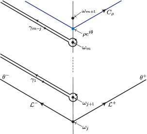
Figure 13: From the Stokes phenomenon to the symbolic Stokes automorphism.

Proof.

It is sufficient to prove it for each homogeneous component of $\Phi$, so we can assume $\Phi=a\,\delta_{\omega_{j}}+\hat{\varphi}\in\raisebox{0.86108pt}[7.96527pt][0.0pt]{${\stackrel{{\scriptstyle\raisebox{-0.60275pt}{$\scriptscriptstyle\triangledown$}}}{{E}}}$}^{I,\gamma}_{\omega_{j}}(\Omega)$, with $0\leq j\leq m$. Given $z\in\mathscr{D}(I_{\epsilon}^{+},\gamma+\epsilon)\cap\mathscr{D}(I_{\epsilon}^{-},\gamma+\epsilon)$, we choose ${\theta}^{+}\in I^{+}$ and ${\theta}^{-}\in I^{-}$ so that ${\zeta}\mapsto\mathrm{e}^{-z{\zeta}}$ is exponentially decreasing on the rays $\mathbb{R}^{+}\mathrm{e}^{{\mathrm{i}}{\theta}^{\pm}}$. Then $\mathcal{L}^{\pm}\Phi(z)$ can be written $a\,\mathrm{e}^{-\omega_{j}z}+\int_{\omega_{j}}^{\mathrm{e}^{{\mathrm{i}}{\theta}^{\pm}}\!\!\infty}\mathrm{e}^{-z{\zeta}}\hat{\varphi}({\zeta})\,{\mathrm{d}}{\zeta}$ (by the very definition of $\tau_{\omega_{j}}$). Decomposing the integration path as indicated on Figure 13, we get

$$\mathcal{L}^{+}\Phi(z)=a\,\mathrm{e}^{-\omega_{j}z}+\Big{(}\int_{\omega_{j}}^{\mathrm{e}^{{\mathrm{i}}{\theta}^{-}}\!\!\infty}+\int_{\gamma_{1}}+\cdots+\int_{\gamma_{m-j}}+\int_{C_{\rho}}\Big{)}\mathrm{e}^{-z{\zeta}}\hat{\varphi}({\zeta})\,{\mathrm{d}}{\zeta}\\ =\mathcal{L}^{-}\Phi(z)+\sum_{r=1}^{m-j}\int_{\gamma_{r}}\mathrm{e}^{-z{\zeta}}\,\raisebox{0.90419pt}{$\stackrel{{\scriptstyle\raisebox{-0.69318pt}{$\scriptscriptstyle\bullet$}}}{{\ell}}_{\raisebox{-0.69318pt}{$\scriptstyle+$}}^{\raisebox{-1.80835pt}{$\,\scriptstyle r-1$}}$}\mu\Phi({\zeta})\,{\mathrm{d}}{\zeta}+\int_{C_{\rho}}\mathrm{e}^{-z{\zeta}}\,\raisebox{0.90419pt}{$\stackrel{{\scriptstyle\raisebox{-0.69318pt}{$\scriptscriptstyle\bullet$}}}{{\ell}}_{\raisebox{-0.69318pt}{$\scriptstyle+$}}^{\raisebox{-1.80835pt}{$\,\scriptstyle m-j-1$}}$}\mu\Phi({\zeta})\,{\mathrm{d}}{\zeta},$$

where the contour $C_{\rho}$ consists of the negatively oriented half-line $[\rho\,\mathrm{e}^{{\mathrm{i}}{\theta}},\mathrm{e}^{{\mathrm{i}}{\theta}^{-}}\!\!\infty)$ followed by the positively oriented half-line $[\rho\,\mathrm{e}^{{\mathrm{i}}{\theta}},\mathrm{e}^{{\mathrm{i}}{\theta}^{+}}\!\!\infty)$. We recognize in the $m-j$ terms of the sum in the right-hand side the Laplace integral of majors (cf. Section 26.1) applied to the homogeneous components of $[{\Delta\raisebox{1.72218pt}{$\scriptscriptstyle/$}\hskip 3.00003pt^{+}_{d}}\Phi]_{m}$; all these integrals are convergent by virtue of our hypothesis that $[{\Delta\raisebox{1.72218pt}{$\scriptscriptstyle/$}\hskip 3.00003pt^{+}_{d}}\Phi]_{m}\in\raisebox{0.86108pt}[7.96527pt][0.0pt]{${\stackrel{{\scriptstyle\raisebox{-0.60275pt}{$\scriptscriptstyle\triangledown$}}}{{E}}}$}^{I,\gamma}(\Omega,d,m)$, and also the last term in the right-hand side is seen to be a convergent integral which yields an $O(\mathrm{e}^{-\rho\mathop{\Re e}\nolimits(\mathrm{e}^{{\mathrm{i}}{\theta}}z)})$ error term. ∎

Observe that the meaning of (153) for $\Phi=\hat{\varphi}\in\raisebox{0.86108pt}[7.96527pt][0.0pt]{${\stackrel{{\scriptstyle\raisebox{-0.60275pt}{$\scriptscriptstyle\triangledown$}}}{{E}}}$}^{I,\gamma}_{0}(\Omega)$, i.e. $\hat{\varphi}\in\hat{\mathscr{R}}_{\Omega}^{\mathrm{simp}}\cap\mathcal{N}(I^{+},\gamma)\cap\mathcal{N}(I^{-},\gamma)$, is

$$\mathcal{L}^{{\theta}^{+}}\hat{\varphi}=\mathcal{L}^{{\theta}^{-}}\hat{\varphi}+\mathrm{e}^{-\omega_{1}z}\mathcal{L}^{{\theta}^{-}}\Delta^{+}_{\omega_{1}}\hat{\varphi}(z)+\cdots+\mathrm{e}^{-\omega_{m}z}\mathcal{L}^{{\theta}^{-}}\Delta^{+}_{\omega_{m}}\hat{\varphi}(z)+O(\mathrm{e}^{-\rho\mathop{\Re e}\nolimits(\mathrm{e}^{{\mathrm{i}}{\theta}}z)}).$$

The idea is that the action of the symbolic Stokes automorphism yields the exponentially small corrections needed to pass from the Borel sum $\mathcal{L}^{{\theta}^{+}}\hat{\varphi}$ to the Borel sum $\mathcal{L}^{{\theta}^{-}}\hat{\varphi}$. It is sometimes possible to pass to the limit $m\to\infty$ and to get rid of any error term, in which case one could be tempted to write

$$\text{``}\mathcal{L}^{+}=\mathcal{L}^{-}\circ{\Delta\raisebox{1.72218pt}{$\scriptscriptstyle/$}\hskip 3.00003pt^{+}_{d}}\text{''}.$$ (154)

Example 29.2.

The simplest example of all is again provided by the Euler series, for which there is only one singular ray, $d=\mathbb{R}^{-}$. Taking any $\Omega\subset\mathbb{R}^{-}$ containing $-1$, we have

$${\Delta\raisebox{1.72218pt}{$\scriptscriptstyle/$}\hskip 3.00003pt^{+}_{\mathbb{R}^{-}}}\hat{\varphi}^{\raisebox{-0.69318pt}{$\scriptstyle\mathrm{E}$}}=\hat{\varphi}^{\raisebox{-0.69318pt}{$\scriptstyle\mathrm{E}$}}+2\pi{\mathrm{i}}\,\delta_{-1}$$ (155)

(in view of (138)). If we set $I^{+}\coloneqq(\frac{\pi}{2},\pi)$ and $I^{-}\coloneqq(\pi,\frac{3\pi}{2})$, then the functions $\varphi^{+}=\mathcal{L}^{+}\hat{\varphi}^{\raisebox{-0.69318pt}{$\scriptstyle\mathrm{E}$}}$ and $\varphi^{-}=\mathcal{L}^{-}\hat{\varphi}^{\raisebox{-0.69318pt}{$\scriptstyle\mathrm{E}$}}$ coincide with those of Section 10. Recall that one can take $\gamma=0$ in this case, so $\varphi^{\pm}$ is holomorphic in $\mathscr{D}(I^{\pm},0)$ (at least) and the intersection $\mathscr{D}(I^{+},0)\cap\mathscr{D}(I^{-},0)$ is the half-plane $\{\mathop{\Re e}\nolimits z<0\}$, on which Theorem 29.5 implies

$$\varphi^{+}=\varphi^{-}+2\pi{\mathrm{i}}\,\mathrm{e}^{z},$$

which is consistent with formula (45).

Example 29.3.

Similarly, for Poincaré’s example with parameter $s\in\mathbb{C}$ of negative real part, according to Section 12, the singular rays are $d_{k}\coloneqq\mathbb{R}^{+}\mathrm{e}^{{\mathrm{i}}{\theta}_{k}}$, $k\in\mathbb{Z}$, with $\omega_{k}=s+2\pi{\mathrm{i}}k$ and ${\theta}_{k}\coloneqq\arg\omega_{k}\in(\frac{\pi}{2},\frac{3\pi}{2})$. We take any $\Omega$ contained the union of these rays and containing $s+2\pi{\mathrm{i}}\mathbb{Z}$. For fixed $k$, we can set $I^{+}\coloneqq J_{k-1}=(\arg\omega_{k-1},\arg\omega_{k})$, $I^{-}\coloneqq J_{k}=(\arg\omega_{k},\arg\omega_{k+1})$, and $\gamma({\theta})\equiv\cos{\theta}$. Then, according to Theorem 12.3, the Borel sums $\mathcal{L}^{+}\hat{\varphi}^{\raisebox{-0.69318pt}{$\scriptstyle\mathrm{P}$}}=\mathscr{S}^{J_{k-1}}\tilde{\varphi}^{\raisebox{-0.69318pt}{$\scriptstyle\mathrm{P}$}}$ and $\mathcal{L}^{-}\hat{\varphi}^{\raisebox{-0.69318pt}{$\scriptstyle\mathrm{P}$}}=\mathscr{S}^{J_{k}}\tilde{\varphi}^{\raisebox{-0.69318pt}{$\scriptstyle\mathrm{P}$}}$ are well defined. In view of (138), we have

$${\Delta\raisebox{1.72218pt}{$\scriptscriptstyle/$}\hskip 3.00003pt^{+}_{d_{k}}}\hat{\varphi}^{\raisebox{-0.69318pt}{$\scriptstyle\mathrm{P}$}}=\hat{\varphi}^{\raisebox{-0.69318pt}{$\scriptstyle\mathrm{P}$}}+2\pi{\mathrm{i}}\,\delta_{\omega_{k}},\quad\text{hence}\quad\mathcal{L}^{+}\hat{\varphi}^{\raisebox{-0.69318pt}{$\scriptstyle\mathrm{P}$}}=\mathcal{L}^{-}\hat{\varphi}^{\raisebox{-0.69318pt}{$\scriptstyle\mathrm{P}$}}+2\pi{\mathrm{i}}\,\mathrm{e}^{-\omega_{k}z}$$

by Theorem 29.5, which is consistent with (66).

Example 29.4.

The asymptotic expansion $\tilde{\varphi}^{\raisebox{-0.69318pt}{$\scriptstyle\mathrm{H}$}}_{s}(z)$ of the Hurwitz zeta function was studied in Exercise 27.5. For $s\geq 2$ integer, with $I=(-\frac{\pi}{2},\frac{\pi}{2})$, we have

$$\varphi^{+}(z)\coloneqq\sum_{k\in\mathbb{N}}(z+k)^{-s}=\mathscr{S}^{I}\tilde{\varphi}^{\raisebox{-0.69318pt}{$\scriptstyle\mathrm{H}$}}_{s}(z)$$

for $z\in\mathscr{D}(I,0)=\mathbb{C}\setminus\mathbb{R}^{-}$. With the help of the difference equation $\varphi(z)-\varphi(z+1)=z^{-s}$, it is an exercise to check that

$$\varphi^{-}(z)\coloneqq-\sum_{k\in\mathbb{N}^{*}}(z-k)^{-s}$$

coincides with the Borel sum $\mathscr{S}^{J}\tilde{\varphi}^{\raisebox{-0.69318pt}{$\scriptstyle\mathrm{H}$}}_{s}$ defined on $\mathscr{D}(J,0)=\mathbb{C}\setminus\mathbb{R}^{+}$, with $J=(\frac{\pi}{2},\frac{3\pi}{2})$ or $(-\frac{3\pi}{2},-\frac{\pi}{2})$. In this case, we can take $\Omega=2\pi{\mathrm{i}}\mathbb{Z}^{*}$ and we have two singular rays, ${\mathrm{i}}\mathbb{R}^{+}$ and ${\mathrm{i}}\mathbb{R}^{-}$, for each of which the symbolic Stokes automorphism yields infinitely many non-trivial homogeneous components: indeed, according to (138),

$${\Delta\raisebox{1.72218pt}{$\scriptscriptstyle/$}\hskip 3.00003pt^{+}_{{\mathrm{i}}\mathbb{R}^{+}}}\hat{\varphi}^{\raisebox{-0.69318pt}{$\scriptstyle\mathrm{H}$}}_{s}=\hat{\varphi}^{\raisebox{-0.69318pt}{$\scriptstyle\mathrm{H}$}}_{s}+\frac{2\pi{\mathrm{i}}}{{\Gamma}(s)}\sum_{m=1}^{\infty}(2\pi{\mathrm{i}}m)^{s-1}\delta_{2\pi{\mathrm{i}}m},\qquad{\Delta\raisebox{1.72218pt}{$\scriptscriptstyle/$}\hskip 3.00003pt^{+}_{{\mathrm{i}}\mathbb{R}^{-}}}\hat{\varphi}^{\raisebox{-0.69318pt}{$\scriptstyle\mathrm{H}$}}_{s}=\hat{\varphi}^{\raisebox{-0.69318pt}{$\scriptstyle\mathrm{H}$}}_{s}+\frac{2\pi{\mathrm{i}}}{{\Gamma}(s)}\sum_{m=1}^{\infty}(-2\pi{\mathrm{i}}m)^{s-1}\delta_{-2\pi{\mathrm{i}}m}.$$

Applying Theorem 29.5 with $I^{+}=(0,\frac{\pi}{2})$ and $I^{-}=(\frac{\pi}{2},\pi)$, or with $I^{+}=(-\pi,-\frac{\pi}{2})$ and $I^{-}=(-\frac{\pi}{2},0)$, for each $m\in\mathbb{N}$ we get

$$\mathop{\Im m}\nolimits z<0\enspace\Longrightarrow\enspace\varphi^{+}(z)=\varphi^{-}(z)+\frac{2\pi{\mathrm{i}}}{{\Gamma}(s)}\sum_{j=1}^{m}(2\pi{\mathrm{i}}j)^{s-1}\mathrm{e}^{-2\pi{\mathrm{i}}jz}+O(\mathrm{e}^{-2\pi(m+\frac{1}{2})\lvert\mathop{\Im m}\nolimits z\rvert}),$$ (156)

$$\mathop{\Im m}\nolimits z>0\enspace\Longrightarrow\enspace\varphi^{-}(z)=\varphi^{+}(z)+\frac{2\pi{\mathrm{i}}}{{\Gamma}(s)}\sum_{j=1}^{m}(-2\pi{\mathrm{i}}j)^{s-1}\mathrm{e}^{2\pi{\mathrm{i}}jz}+O(\mathrm{e}^{-2\pi(m+\frac{1}{2})\lvert\mathop{\Im m}\nolimits z\rvert})$$ (157)

(and the constants implied in these estimates are uniform provided one restricts oneself to $\lvert z\rvert>\epsilon$ and $\lvert\arg z\pm{\mathrm{i}}\frac{\pi}{2}\rvert<\frac{\pi}{2}-\epsilon$). In this case we see that we can pass to the limit $m\to\infty$ because the finite sums involved in (156)–(157) are the partial sums of convergent series. In fact this could be guessed in advance: since $\varphi^{+}$ and $\varphi^{-}$ satisfy the same difference equation $\varphi(z)-\varphi(z+1)=z^{-s}$, their difference yields $1$-periodic functions holomorphic in the half-planes $\{\mathop{\Im m}\nolimits z<0\}$ and $\{\mathop{\Im m}\nolimits z>0\}$, which thus have convergent Fourier series of the form

$$(\varphi^{+}-\varphi^{-})_{|\{\mathop{\Im m}\nolimits z<0\}}=\sum_{m\geq 0}A_{m}\mathrm{e}^{-2\pi{\mathrm{i}}mz},\qquad(\varphi^{+}-\varphi^{-})_{|\{\mathop{\Im m}\nolimits z>0\}}=\sum_{m\geq 0}B_{m}\mathrm{e}^{2\pi{\mathrm{i}}mz},$$

but the finite sums in (156)–(157) are nothing but the partial sums of these series (up to sign for the second). So, in this case, the symbolic Stokes automorphism delivers the Fourier coefficients of the diffence between the two Borel sums:

$$\sum_{k\in\mathbb{Z}}(z+k)^{-s}=\begin{cases}\displaystyle\tfrac{2\pi{\mathrm{i}}}{{\Gamma}(s)}\sum_{m=1}^{\infty}(2\pi{\mathrm{i}}m)^{s-1}\mathrm{e}^{-2\pi{\mathrm{i}}mz}&\text{for $\mathop{\Im m}\nolimits z<0$,}\\[8.61108pt] \displaystyle\tfrac{2\pi{\mathrm{i}}}{{\Gamma}(s)}\sum_{m=1}^{\infty}(-1)^{s}(2\pi{\mathrm{i}}m)^{s-1}\mathrm{e}^{2\pi{\mathrm{i}}mz}&\text{for $\mathop{\Im m}\nolimits z>0$.}\end{cases}$$

Example 29.5.

The case of the Stirling series $\tilde{\mu}$ studied in Section 11 is somewhat similar, with (138) yielding

$${\Delta\raisebox{1.72218pt}{$\scriptscriptstyle/$}\hskip 3.00003pt^{+}_{{\mathrm{i}}\mathbb{R}^{+}}}\hat{\mu}=\hat{\mu}+\sum_{m\in\mathbb{N}^{*}}\frac{1}{m}\,\delta_{2\pi{\mathrm{i}}m},\qquad{\Delta\raisebox{1.72218pt}{$\scriptscriptstyle/$}\hskip 3.00003pt^{+}_{{\mathrm{i}}\mathbb{R}^{-}}}\hat{\mu}=\hat{\mu}-\sum_{m\in\mathbb{N}^{*}}\frac{1}{m}\,\delta_{-2\pi{\mathrm{i}}m}.$$ (158)

Here we get

$$\mathop{\Im m}\nolimits z<0\enspace \Longrightarrow\enspace\mu^{+}(z)=\mu^{-}(z)+\sum_{m=1}^{\infty}\tfrac{1}{m}\mathrm{e}^{-2\pi{\mathrm{i}}mz}=\mu^{-}(z)-\log(1-\mathrm{e}^{-2\pi{\mathrm{i}}z}),$$ (159)

$$\mathop{\Im m}\nolimits z>0\enspace \Longrightarrow\enspace\mu^{-}(z)=\mu^{+}(z)-\sum_{m=1}^{\infty}\tfrac{1}{m}\mathrm{e}^{2\pi{\mathrm{i}}mz}=\mu^{+}(z)+\log(1-\mathrm{e}^{2\pi{\mathrm{i}}z})$$ (160)

(compare with Exercise 11.2).

29.4 Extension of the inverse Borel transform to $\Omega$-resurgent symbols

In the previous section, we have defined the Laplace operators $\mathcal{L}^{+}$ and $\mathcal{L}^{-}$ on

$$\raisebox{0.86108pt}[7.96527pt][0.0pt]{${\stackrel{{\scriptstyle\raisebox{-0.60275pt}{$\scriptscriptstyle\triangledown$}}}{{E}}}$}^{I,\gamma}(\Omega,d,m)\subset\raisebox{0.86108pt}{${\stackrel{{\scriptstyle\raisebox{-0.60275pt}{$\scriptscriptstyle\triangledown$}}}{{E}}}$}(\Omega,d,m)\subset\raisebox{0.86108pt}{${\stackrel{{\scriptstyle\raisebox{-0.60275pt}{$\scriptscriptstyle\triangledown$}}}{{E}}}$}(\Omega,d),$$

i.e. the $\Omega$-resurgent symbols to which they can be applied are subjected to two constraints: finitely many non-trivial homogeneous components, with at most exponential growth at infinity for their minors. There is a natural way to define on the whole of $\raisebox{0.86108pt}{${\stackrel{{\scriptstyle\raisebox{-0.60275pt}{$\scriptscriptstyle\triangledown$}}}{{E}}}$}(\Omega,d)$ a formal Laplace operator, which is an extension of the inverse Borel transform $\mathcal{B}^{-1}$ on $\mathbb{C}\,\delta\oplus\hat{\mathscr{R}}_{\Omega}^{\mathrm{simp}}$. Indeed, replacing the function $\mathrm{e}^{-\omega z}=\mathcal{L}^{\pm}\delta_{\omega}$ by a symbol $\mathrm{e}^{-\omega z}$, we define

$$\tilde{E}_{\omega}(\Omega)\coloneqq\mathrm{e}^{-\omega z}\tilde{\mathscr{R}}_{-\omega+\Omega}^{\mathrm{simp}}\quad\text{for}\enspace\omega\in\Omega\cap d,\qquad\tilde{E}(\Omega,d)\coloneqq\stackrel{{\scriptstyle\raisebox{-0.60275pt}{$\scriptscriptstyle\wedge$}}}{{\displaystyle\bigoplus_{\omega\in\Omega\cap d}}}\tilde{E}_{\omega}(\Omega),$$ (161)

i.e. we take the completed graded vector space obtained as cartesian product of the spaces $\tilde{\mathscr{R}}_{-\omega+\Omega}^{\mathrm{simp}}$, representing its elements by formal expressions of the form $\tilde{\Phi}=\sum_{\omega\in\Omega\cap d}\mathrm{e}^{-\omega z}\tilde{\Phi}_{\omega}(z)$, where each $\tilde{\Phi}_{\omega}(z)$ is a formal series and $\mathrm{e}^{-\omega z}$ is just a symbol meant to distinguish the various homogeneous components. We thus have for each $\omega\in\Omega\cap d$ a linear isomorphism

$$\tilde{\tau}_{\omega}\colon\thinspace\tilde{\varphi}(z)\in\tilde{\mathscr{R}}_{-\omega+\Omega}^{\mathrm{simp}}\mapsto\mathrm{e}^{-\omega z}\tilde{\varphi}(z)\in\tilde{E}_{\omega}(\Omega),$$

which allow us to define

$$\mathcal{B}_{\omega}\coloneqq\tau_{\omega}\circ\mathcal{B}\circ\tilde{\tau}_{\omega}^{-1}\colon\thinspace\tilde{E}_{\omega}(\Omega)\xrightarrow{\sim}\raisebox{0.86108pt}{${\stackrel{{\scriptstyle\raisebox{-0.60275pt}{$\scriptscriptstyle\triangledown$}}}{{E}}}$}_{\omega}(\Omega).$$

The map $\mathcal{B}_{0}$ can be identified with the Borel transform $\mathcal{B}$ acting on simple $\Omega$-resurgent series; putting together the maps $\mathcal{B}_{\omega}$, $\omega\in\Omega\cap d$, we get a linear isomorphism

$$\mathcal{B}\colon\thinspace\tilde{E}(\Omega,d)\xrightarrow{\sim}\raisebox{0.86108pt}{${\stackrel{{\scriptstyle\raisebox{-0.60275pt}{$\scriptscriptstyle\triangledown$}}}{{E}}}$}(\Omega,d),$$

which we can consider as the Borel transform acting on “$\Omega$-resurgent transseries in the direction $d$”, and whose inverse can be considered as the formal Laplace transform acting on $\Omega$-resurgent symbols in the direction $d$.

Observe that, if $\mathrm{e}^{-\omega z}\tilde{\varphi}(z)\in\tilde{E}_{\omega}(\Omega)$ is such that $\tilde{\varphi}(z)$ is $1$-summable in the directions of $I^{+}\cup I^{-}$, then $\mathcal{B}(\mathrm{e}^{-\omega z}\tilde{\varphi})\in\raisebox{0.86108pt}[7.96527pt][0.0pt]{${\stackrel{{\scriptstyle\raisebox{-0.60275pt}{$\scriptscriptstyle\triangledown$}}}{{E}}}$}^{I,\gamma}_{\omega}(\Omega)$ and

$$\mathcal{L}^{\pm}\mathcal{B}(\mathrm{e}^{-\omega z}\tilde{\varphi})=\mathrm{e}^{-\omega z}\mathscr{S}^{I^{\pm}}\tilde{\varphi}.$$

Beware that in the above identity, $\mathrm{e}^{-\omega z}$ is a symbol in the left-hand side, whereas it is a function in the right-hand side.

Via $\mathcal{B}$, the operators ${\Delta\raisebox{1.72218pt}{$\scriptscriptstyle/$}\hskip 3.00003pt^{+}_{d}}$ and ${\Delta\raisebox{1.72218pt}{$\scriptscriptstyle/$}\hskip 3.00003pt_{d}}$ give rise to operators which we denote with the same symbols:

$${\Delta\raisebox{1.72218pt}{$\scriptscriptstyle/$}\hskip 3.00003pt^{+}_{d}},{\Delta\raisebox{1.72218pt}{$\scriptscriptstyle/$}\hskip 3.00003pt_{d}}\colon\thinspace\tilde{E}(\Omega,d)\to\tilde{E}(\Omega,d),$$

so that we can e.g. rephrase (155) as

$${\Delta\raisebox{1.72218pt}{$\scriptscriptstyle/$}\hskip 3.00003pt^{+}_{\mathbb{R}^{-}}}\tilde{\varphi}^{\raisebox{-0.69318pt}{$\scriptstyle\mathrm{E}$}}=\tilde{\varphi}^{\raisebox{-0.69318pt}{$\scriptstyle\mathrm{E}$}}+2\pi{\mathrm{i}}\,\mathrm{e}^{z}$$ (162)

or (158) as

$${\Delta\raisebox{1.72218pt}{$\scriptscriptstyle/$}\hskip 3.00003pt^{+}_{{\mathrm{i}}\mathbb{R}^{+}}}\tilde{\mu}=\tilde{\mu}+\sum_{m\in\mathbb{N}^{*}}\frac{1}{m}\,\mathrm{e}^{-2\pi{\mathrm{i}}mz},\qquad{\Delta\raisebox{1.72218pt}{$\scriptscriptstyle/$}\hskip 3.00003pt^{+}_{{\mathrm{i}}\mathbb{R}^{-}}}\tilde{\mu}=\tilde{\mu}-\sum_{m\in\mathbb{N}^{*}}\frac{1}{m}\,\mathrm{e}^{2\pi{\mathrm{i}}mz}.$$ (163)

In Section 30.2, we shall see that, if $\Omega$ is stable under addition, then $\raisebox{0.86108pt}{${\stackrel{{\scriptstyle\raisebox{-0.60275pt}{$\scriptscriptstyle\triangledown$}}}{{E}}}$}(\Omega,d)$ and thus also $\tilde{E}(\Omega,d)$ have algebra structures, for which it is legitimate to write

$$-\log(1-\mathrm{e}^{-2\pi{\mathrm{i}}z})=\sum_{m\in\mathbb{N}^{*}}\frac{1}{m}\,\mathrm{e}^{-2\pi{\mathrm{i}}mz},\quad\log(1-\mathrm{e}^{2\pi{\mathrm{i}}z})=-\sum_{m\in\mathbb{N}^{*}}\frac{1}{m}\,\mathrm{e}^{2\pi{\mathrm{i}}mz}.$$ (164)

Remark 29.6.

One can always extend the definition of $\partial=\frac{{\mathrm{d}}\,}{{\mathrm{d}}z}$ to $\tilde{E}(\Omega,d)$ by setting

$$\tilde{\varphi}\in\tilde{\mathscr{R}}_{-\omega+\Omega}^{\mathrm{simp}}\enspace\Longrightarrow\enspace\partial(\mathrm{e}^{-\omega z}\tilde{\varphi})\coloneqq\mathrm{e}^{-\omega z}(-\omega+\partial)\tilde{\varphi}.$$

(When $\Omega$ is stable under addition $\partial$ will be a derivation of the algebra $\tilde{E}(\Omega,d)$, which will thus be a differential algebra.)

On the other hand, writing as usual $\Omega\cap d=\{0=\omega_{0}\prec\omega_{1}\prec\omega_{2}\prec\cdots\}$, we see that the homogeneous components of ${\Delta\raisebox{1.72218pt}{$\scriptscriptstyle/$}\hskip 3.00003pt^{+}_{d}}$ and ${\Delta\raisebox{1.72218pt}{$\scriptscriptstyle/$}\hskip 3.00003pt_{d}}$ acting on $\tilde{E}(\Omega,d)$ (Borel counterparts of the operators $\raisebox{0.99025pt}{ {$\stackrel{{\scriptstyle\raisebox{-0.69318pt}{$\scriptscriptstyle\bullet$}}}{{\Delta}}_{\raisebox{-0.69318pt}{$\scriptstyle r$}}^{\raisebox{-2.56181pt}{$\scriptstyle+$}}$}},\,\raisebox{0.99025pt}{ {$\stackrel{{\scriptstyle\raisebox{-0.69318pt}{$\scriptscriptstyle\bullet$}}}{{\Delta}}_{\raisebox{-0.69318pt}[3.01389pt][0.0pt]{$\scriptstyle r$}}$}}\colon\thinspace\raisebox{0.86108pt}{${\stackrel{{\scriptstyle\raisebox{-0.60275pt}{$\scriptscriptstyle\triangledown$}}}{{E}}}$}\to\raisebox{0.86108pt}{${\stackrel{{\scriptstyle\raisebox{-0.60275pt}{$\scriptscriptstyle\triangledown$}}}{{E}}}$}$ defined by (148)) act as follows on $\tilde{E}_{\omega}(\Omega)$ for each $\omega=\omega_{m}\in\Omega\cap d$:

$$\tilde{\varphi}\in\tilde{\mathscr{R}}_{-\omega_{m}+\Omega}^{\mathrm{simp}}\enspace\Longrightarrow\enspace\left\{\begin{aligned} \raisebox{0.99025pt}{ {$\stackrel{{\scriptstyle\raisebox{-0.69318pt}{$\scriptscriptstyle\bullet$}}}{{\Delta}}_{\raisebox{-0.69318pt}{$\scriptstyle r$}}^{\raisebox{-2.56181pt}{$\scriptstyle+$}}$}}(\mathrm{e}^{-\omega_{m}z}\tilde{\varphi})&=\mathrm{e}^{-\omega_{m+r}z}\Delta^{+}_{\omega_{m+r}-\omega_{m}}\tilde{\varphi},\\[4.30554pt] \enspace\raisebox{0.99025pt}{ {$\stackrel{{\scriptstyle\raisebox{-0.69318pt}{$\scriptscriptstyle\bullet$}}}{{\Delta}}_{\raisebox{-0.69318pt}[3.01389pt][0.0pt]{$\scriptstyle r$}}$}}(\mathrm{e}^{-\omega_{m}z}\tilde{\varphi})&=\mathrm{e}^{-\omega_{m+r}z}\Delta_{\omega_{m+r}-\omega_{m}}\tilde{\varphi}.\end{aligned}\right.$$ (165)

Formula (139) then says

$$\raisebox{0.99025pt}{ {$\stackrel{{\scriptstyle\raisebox{-0.69318pt}{$\scriptscriptstyle\bullet$}}}{{\Delta}}_{\raisebox{-0.69318pt}{$\scriptstyle r$}}^{\raisebox{-2.56181pt}{$\scriptstyle+$}}$}}\partial\phi=\partial\raisebox{0.99025pt}{ {$\stackrel{{\scriptstyle\raisebox{-0.69318pt}{$\scriptscriptstyle\bullet$}}}{{\Delta}}_{\raisebox{-0.69318pt}{$\scriptstyle r$}}^{\raisebox{-2.56181pt}{$\scriptstyle+$}}$}}\phi,\quad\raisebox{0.99025pt}{ {$\stackrel{{\scriptstyle\raisebox{-0.69318pt}{$\scriptscriptstyle\bullet$}}}{{\Delta}}_{\raisebox{-0.69318pt}[3.01389pt][0.0pt]{$\scriptstyle r$}}$}}\partial\phi=\partial\raisebox{0.99025pt}{ {$\stackrel{{\scriptstyle\raisebox{-0.69318pt}{$\scriptscriptstyle\bullet$}}}{{\Delta}}_{\raisebox{-0.69318pt}[3.01389pt][0.0pt]{$\scriptstyle r$}}$}}\phi$$

for every $\phi\in\tilde{E}(\Omega,d)$, whence ${\Delta\raisebox{1.72218pt}{$\scriptscriptstyle/$}\hskip 3.00003pt^{+}_{d}}\circ\partial=\partial\circ{\Delta\raisebox{1.72218pt}{$\scriptscriptstyle/$}\hskip 3.00003pt^{+}_{d}}$ and ${\Delta\raisebox{1.72218pt}{$\scriptscriptstyle/$}\hskip 3.00003pt_{d}}\circ\partial=\partial\circ{\Delta\raisebox{1.72218pt}{$\scriptscriptstyle/$}\hskip 3.00003pt_{d}}$.

30 The operators $\Delta_{\omega}$ are derivations

We now investigate the way the operators $\Delta_{\omega}$ and $\Delta^{+}_{\omega}$ act on a product of two terms (convolution product or Cauchy product, according as one works with formal series or their Borel transforms).

Let $\Omega^{\prime}$ and $\Omega^{\prime\prime}$ be non-empty closed discrete subsets of $\mathbb{C}$ such that

$$\Omega\coloneqq\Omega^{\prime}\cup\Omega^{\prime\prime}\cup(\Omega^{\prime}+\Omega^{\prime\prime})$$ (166)

is also closed and discrete. Recall that, according to Theorem 21.8,

$$\tilde{\varphi}\in\tilde{\mathscr{R}}_{\Omega^{\prime}}\enspace\text{and}\enspace\tilde{\psi}\in\tilde{\mathscr{R}}_{\Omega^{\prime\prime}}\quad\Longrightarrow\quad\tilde{\varphi}\tilde{\psi}\in\tilde{\mathscr{R}}_{\Omega}.$$

30.1 Generalized Leibniz rule for the operators $\Delta^{+}_{\omega}$

We begin with the operators $\Delta^{+}_{\omega}$.

Theorem 30.1.

Let $\tilde{\varphi}\in\tilde{\mathscr{R}}_{\Omega^{\prime}}^{\mathrm{simp}}$ and $\tilde{\psi}\in\tilde{\mathscr{R}}_{\Omega^{\prime\prime}}^{\mathrm{simp}}$. Then $\tilde{\varphi}\tilde{\psi}\in\tilde{\mathscr{R}}_{\Omega}^{\mathrm{simp}}$ and, for every $\omega\in\Omega\setminus\{0\}$,

$$\Delta^{+}_{\omega}(\tilde{\varphi}\tilde{\psi})=(\Delta^{+}_{\omega}\tilde{\varphi})\tilde{\psi}+\sum_{\begin{subarray}{c}\omega=\omega^{\prime}+\omega^{\prime\prime}\\ \omega^{\prime}\in\Omega^{\prime}\cap{]0,\omega[},\,\omega^{\prime\prime}\in\Omega^{\prime\prime}\cap{]0,\omega[}\end{subarray}}(\Delta^{+}_{\omega^{\prime}}\tilde{\varphi})(\Delta^{+}_{\omega^{\prime\prime}}\tilde{\psi})\quad+\;\tilde{\varphi}(\Delta^{+}_{\omega}\tilde{\psi}).$$ (167)

Proof.

a) The fact that $\tilde{\varphi}\tilde{\psi}\in\tilde{\mathscr{R}}_{\Omega}^{\mathrm{simp}}$ follows from the proof of formula (167) and Theorem 28.7, we omit the details.

b) To prove formula (167), we define

$${\Sigma}_{\omega}\coloneqq\{\,\eta\in{]0,\omega[}\mid\eta\in\Omega^{\prime}\cup\Omega^{\prime\prime}\;\text{or}\;\omega-\eta\in\Omega^{\prime}\cup\Omega^{\prime\prime}\,\}$$

and write $\mathcal{B}\tilde{\varphi}=a\,\delta+\hat{\varphi}$, $\mathcal{B}\tilde{\psi}=b\,\delta+\hat{\psi}$, with $a,b\in\mathbb{C}$, $\hat{\varphi}\in\hat{\mathscr{R}}_{\Omega^{\prime}}^{\mathrm{simp}}$, $\hat{\psi}\in\hat{\mathscr{R}}_{\Omega^{\prime\prime}}^{\mathrm{simp}}$,

$$\mathcal{B}\Delta^{+}_{\eta}\tilde{\varphi} =a_{\eta}\,\delta+\hat{\varphi}_{\eta}, a_{\eta}\in\mathbb{C},\enspace\hat{\varphi}_{\eta}\in\hat{\mathscr{R}}_{-\eta+\Omega^{\prime}}^{\mathrm{simp}}, \eta\in{\Sigma}_{\omega}\cup\{\omega\}$$ (168)

$$\mathcal{B}\Delta^{+}_{\omega-\eta}\tilde{\psi} =b_{\omega-\eta}\,\delta+\hat{\psi}_{\omega-\eta}, b_{\omega-\eta}\in\mathbb{C},\enspace\hat{\psi}_{\omega-\eta}\in\hat{\mathscr{R}}_{-(\omega-\eta)+\Omega^{\prime\prime}}^{\mathrm{simp}}, \eta\in\{0\}\cup{\Sigma}_{\omega}.$$ (169)

Since $\mathcal{B}\Delta^{+}_{\omega}(\tilde{\varphi}\tilde{\psi})=b\Delta^{+}_{\omega}\hat{\varphi}+a\Delta^{+}_{\omega}\hat{\psi}+\Delta^{+}_{\omega}(\hat{\varphi}*\hat{\psi})$, formula (167) is equivalent to

$$\Delta^{+}_{\omega}(\hat{\varphi}*\hat{\psi})=\sum_{\eta\in\{0,\omega\}\cup{\Sigma}_{\omega}}(a_{\eta}\,\delta+\hat{\varphi}_{\eta})*(b_{\omega-\eta}\,\delta+\hat{\psi}_{\omega-\eta}),$$ (170)

with the convention $a_{0}=0$, $\hat{\varphi}_{0}=\hat{\varphi}$ and $b_{0}=0$, $\hat{\psi}_{0}=\hat{\psi}$.

Consider a neighbourhood of $[0,\omega]$ of the form $U_{\delta}=\{\,{\zeta}\in\mathbb{C}\mid\operatorname{dist}\big{(}{\zeta},[0,\omega]\big{)}<\delta\,\}$ with $\delta>0$ small enough so that $U_{\delta}\setminus[0,\omega]$ does not meet $\Omega$. Let $u\coloneqq\omega\,\mathrm{e}^{-{\mathrm{i}}\alpha}$ with $0<\alpha<\frac{\pi}{2}$, $\alpha$ small enough so that $u\in U_{\delta}$ and the line segment $\ell\coloneqq[0,u]$ can be considered as a path issuing from $0$ circumventing to the right all the points of ${]0,\omega[}\cup\Omega$. We must show that $\operatorname{cont}_{\ell}(\hat{\varphi}*\hat{\psi})(\omega+{\zeta})$ has a simple singularity at $0$ and compute this singularity.

c) We shall show that, when all the numbers $a_{\eta}$ and $b_{\omega-\eta}$ vanish,

$$f({\zeta})\coloneqq\operatorname{cont}_{\ell}(\hat{\varphi}*\hat{\psi})(\omega+{\zeta})=\Bigg{(}\sum_{\eta\in\{0,\omega\}\cup{\Sigma}_{\omega}}\hat{\varphi}_{\eta}*\hat{\psi}_{\omega-\eta}\Bigg{)}\frac{\mathrm{\mathscr{L}og\hskip 1.5pt}{\zeta}}{2\pi{\mathrm{i}}}+R({\zeta}),$$ (171)

where $\mathrm{\mathscr{L}og\hskip 1.5pt}{\zeta}$ is a branch of the logarithm and $R({\zeta})\in\mathbb{C}\{{\zeta}\}$. This is sufficient to conclude, because in the general case we can write

$$\hat{\varphi}*\hat{\psi}=\big{(}\tfrac{{\mathrm{d}}\,}{{\mathrm{d}}{\zeta}}\big{)}^{2}(\hat{\varphi}^{*}*\hat{\psi}^{*}),\qquad\hat{\varphi}^{*}\coloneqq 1*\hat{\varphi},\enspace\hat{\psi}^{*}\coloneqq 1*\hat{\psi},$$

and, by Theorem 27.9, the anti-derivatives $\hat{\varphi}^{*}$ and $\hat{\psi}^{*}$ satisfy

$$\Delta^{+}_{\eta}\hat{\varphi}^{*}=a_{\eta}+1*\hat{\varphi}_{\eta},\qquad\Delta^{+}_{\omega-\eta}\hat{\psi}^{*}=b_{\omega-\eta}+1*\hat{\psi}_{\omega-\eta}$$

instead of (168)–(169), thus we can apply (171) to them and get

$$\operatorname{cont}_{\ell}(\hat{\varphi}^{*}*\hat{\psi}^{*})(\omega+{\zeta})=\Bigg{(}\sum_{\eta\in\{0,\omega\}\cup{\Sigma}_{\omega}}a_{\eta}b_{\omega-\eta}\,{\zeta}+a_{\eta}\,{\zeta}*\hat{\psi}_{\omega-\eta}+b_{\omega-\eta}\,{\zeta}*\hat{\varphi}_{\eta}+{\zeta}*\hat{\varphi}_{\eta}*\hat{\psi}_{\omega-\eta}\Bigg{)}\frac{\mathrm{\mathscr{L}og\hskip 1.5pt}{\zeta}}{2\pi{\mathrm{i}}}\\[4.30554pt] +R({\zeta}),$$

whence, by differentiating twice, a formula whose interpretation is precisely (170) (because $(\frac{{\mathrm{d}}\,}{{\mathrm{d}}{\zeta}}({\zeta}*A))/{\zeta}$ and $({\zeta}*A)/{{\zeta}^{2}}$ are regular at $0$ for whatever regular germ $A$).

d) From ow on, we thus suppose that all the numbers $a_{\eta}$ and $b_{\omega-\eta}$ vanish. Our aim is to prove (171). We observe that $D^{+}\coloneqq\{\,{\zeta}\in D(\omega,\delta)\mid\mathop{\Im m}\nolimits({\zeta}/\omega)<0\,\}$ is a half-disc such that, for all ${\zeta}\in D^{+}$, the line segment $[0,{\zeta}]$ does not meet $\Omega\setminus\{0\}$, hence $\operatorname{cont}_{\ell}(\hat{\varphi}*\hat{\psi})({\zeta})=\int_{0}^{\zeta}\hat{\varphi}(\xi)\hat{\psi}({\zeta}-\xi)\,{\mathrm{d}}\xi$ for such points. We know by Section 21 that $f$ has spiral continuation around $0$. Following the ideas of Section 25, we choose a determination of $\arg\omega$ and lift the half-disc $-\omega+D^{+}$ to the Riemann surface of logarithm by setting $\tilde{D}^{+}\coloneqq\{\,{\zeta}=r\,{\underline{\mathrm{e}}}^{{\mathrm{i}}{\theta}}\in\tilde{\mathbb{C}}\mid r<\delta,\ \arg\omega-\pi<{\theta}<\arg\omega\,\}$. This way we can write $f={\stackrel{{\scriptstyle\raisebox{-0.69318pt}{$\scriptscriptstyle\vee$}}}{{f}}}\circ\pi$, where ${\stackrel{{\scriptstyle\raisebox{-0.69318pt}{$\scriptscriptstyle\vee$}}}{{f}}}$ is a representative of a singular germ, explicitly defined on $\tilde{D}^{+}$ by

$${\zeta}\in\tilde{D}^{+}\enspace\Longrightarrow\enspace{\stackrel{{\scriptstyle\raisebox{-0.69318pt}{$\scriptscriptstyle\vee$}}}{{f}}}({\zeta})=\int_{\ell_{\pi({\zeta})}}\hat{\varphi}(\xi)\hat{\psi}(\omega+\pi({\zeta})-\xi)\,{\mathrm{d}}\xi\quad\text{with $\ell_{\pi({\zeta})}\coloneqq[0,\omega+\pi({\zeta})]$.}$$ (172)

The analytic continuation of ${\stackrel{{\scriptstyle\raisebox{-0.69318pt}{$\scriptscriptstyle\vee$}}}{{f}}}$ in

$$\tilde{D}^{-}\coloneqq\{\,{\zeta}=r\,{\underline{\mathrm{e}}}^{{\mathrm{i}}{\theta}}\in\tilde{\mathbb{C}}\mid r<\delta,\ \arg\omega-3\pi<{\theta}\leq\arg\omega-\pi\,\}$$

is given by

$${\zeta}\in\tilde{D}^{-}\enspace\Longrightarrow\enspace{\stackrel{{\scriptstyle\raisebox{-0.69318pt}{$\scriptscriptstyle\vee$}}}{{f}}}({\zeta})=\int_{L_{\pi({\zeta})}}\hat{\varphi}(\xi)\hat{\psi}(\omega+\pi({\zeta})-\xi)\,{\mathrm{d}}\xi,$$ (173)

where the symmetrically contractible path $L_{\pi({\zeta})}$ is obtained by following the principles expounded in Section 21 (cf. particularly (109)); this is illustrated in Figure 14.

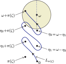
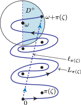
Figure 14: Integration paths for $\hat{\varphi}*\hat{\psi}$. Left: $L_{\pi({\zeta})}$ for $\arg\omega-2\pi<\arg{\zeta}\leq\arg\omega-\pi$.
Right: $\ell_{\pi({\zeta})}$ and $L_{\pi({\zeta})}$ for $\arg\omega-3\pi<\arg{\zeta}\leq\arg\omega-2\pi$. (Case when ${\Sigma}_{\omega}$ has two elements.)

We first show that

$${\zeta}\in\tilde{D}^{+}\enspace\Longrightarrow\enspace{\stackrel{{\scriptstyle\raisebox{-0.69318pt}{$\scriptscriptstyle\vee$}}}{{f}}}({\zeta})-{\stackrel{{\scriptstyle\raisebox{-0.69318pt}{$\scriptscriptstyle\vee$}}}{{f}}}({\zeta}\,{\underline{\mathrm{e}}}^{-2\pi{\mathrm{i}}})=\sum_{\eta\in\{0,\omega\}\cup{\Sigma}_{\omega}}\hat{\varphi}_{\eta}*\hat{\psi}_{\omega-\eta}.$$ (174)

The point is that ${\Sigma}_{\omega}$ is symmetric with respect to its midpoint $\frac{\omega}{2}$, thus of the form $\{\eta_{1}\prec\cdots\eta_{r-1}\}$ with $\eta_{r-j}=\omega-\eta_{j}$ for each $j$, and when ${\zeta}$ travels along a small circle around $\omega$, the “moving nail” ${\zeta}-\eta_{j}$ turns around the “fixed nail” $\eta_{r-j}$, to use the language of Section 21.7. Thus, for ${\zeta}\in\tilde{D}^{+}$, we can decompose the difference of paths $\ell_{\pi({\zeta})}-L_{\pi({\zeta})}$ as on Figure 15 and get

$${\stackrel{{\scriptstyle\raisebox{-0.69318pt}{$\scriptscriptstyle\vee$}}}{{f}}}({\zeta})-{\stackrel{{\scriptstyle\raisebox{-0.69318pt}{$\scriptscriptstyle\vee$}}}{{f}}}({\zeta}\,{\underline{\mathrm{e}}}^{-2\pi{\mathrm{i}}})=\bigg{(}\int_{\pi({\zeta})-\gamma}+\int_{\omega+\gamma}+\sum_{\eta\in{\Sigma}_{\omega}}\int_{\eta+{\Gamma}}\bigg{)}\hat{\varphi}(\xi)\hat{\psi}(\omega+\pi({\zeta})-\xi)\,{\mathrm{d}}\xi,$$

where $\gamma$ goes from ${\zeta}\,{\underline{\mathrm{e}}}^{-2\pi{\mathrm{i}}}$ to ${\zeta}$ by turning anticlockwise around $0$, whereas ${\Gamma}$ goes from ${\zeta}\,{\underline{\mathrm{e}}}^{-2\pi{\mathrm{i}}}$ to ${\zeta}$ the same way but then comes back to ${\zeta}\,{\underline{\mathrm{e}}}^{-2\pi{\mathrm{i}}}$ (see Figure 15).

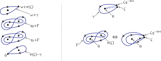
Figure 15: Computation of the variation of the singularity at $\omega$ of $\hat{\varphi}*\hat{\psi}$.

With an appropriate change of variable in each of these integrals, this can be rewritten as

$${\stackrel{{\scriptstyle\raisebox{-0.69318pt}{$\scriptscriptstyle\vee$}}}{{f}}}({\zeta})-{\stackrel{{\scriptstyle\raisebox{-0.69318pt}{$\scriptscriptstyle\vee$}}}{{f}}}({\zeta}\,{\underline{\mathrm{e}}}^{-2\pi{\mathrm{i}}})=\int_{\gamma}\hat{\varphi}(\pi({\zeta})-\xi)\hat{\psi}(\omega+\xi)\,{\mathrm{d}}\xi+\int_{\gamma}\hat{\varphi}(\omega+\xi)\hat{\psi}(\pi({\zeta})-\xi)\,{\mathrm{d}}\xi\\[4.30554pt] +\sum_{\eta\in{\Sigma}_{\omega}}\int_{\Gamma}\hat{\varphi}(\eta+\xi)\hat{\psi}(\omega-\eta+\pi({\zeta})-\xi)\,{\mathrm{d}}\xi.$$

In the first two integrals, since

$$\hat{\psi}(\omega+\xi)=\frac{1}{2\pi{\mathrm{i}}}\hat{\psi}_{\omega}(\xi)\mathrm{\mathscr{L}og\hskip 1.5pt}\xi+R^{\prime}(\xi),\qquad\hat{\varphi}(\omega+\xi)=\frac{1}{2\pi{\mathrm{i}}}\hat{\varphi}_{\omega}(\xi)\mathrm{\mathscr{L}og\hskip 1.5pt}\xi+R^{\prime\prime}(\xi),$$

with $R^{\prime}$ and $R^{\prime\prime}$ regular at $0$, and we can diminish $\delta$ so that $\xi$ and $\pi({\zeta})-\xi$ stay in a neighbourhood of $0$ where $\hat{\varphi}$, $\hat{\psi}_{\omega}$, $R^{\prime}$, $\hat{\varphi}_{\omega}$, $R^{\prime\prime}$ and $\hat{\psi}$ are holomorphic, the Cauchy theorem cancels the contribution of $R^{\prime}$ and $R^{\prime\prime}$, while the contribution of the logarithms can be computed by collapsing $\gamma$ onto the line segment $[{\zeta}\,{\underline{\mathrm{e}}}^{-2\pi{\mathrm{i}}},0]$ followed by $[0,{\zeta}]$, hence the sum of the first two integrals is $\hat{\varphi}*\hat{\psi}_{\omega}+\hat{\varphi}_{\omega}*\hat{\psi}$. Similarly, by collapsing ${\Gamma}$ as indicated on Figure 15,

$$\int_{\Gamma}\hat{\varphi}(\eta+\xi)\hat{\psi}(\omega-\eta+\pi({\zeta})-\xi)\,{\mathrm{d}}\xi=\frac{1}{2\pi{\mathrm{i}}}\int_{\Gamma}\hat{\varphi}(\eta+\xi)\big{(}\hat{\psi}_{\omega-\eta}(\pi({\zeta})-\xi)\mathrm{\mathscr{L}og\hskip 1.5pt}\xi+R_{\omega-\eta}(\xi)\big{)}\,{\mathrm{d}}\xi$$

(with some regular germ $R_{\omega-\eta}$) is seen to coincide with $\int_{\gamma}\hat{\varphi}(\eta+\xi)\hat{\psi}_{\omega-\eta}(\pi({\zeta})-\xi)\,{\mathrm{d}}\xi$, which is itself seen to coincide with $\hat{\varphi}_{\eta}*\hat{\psi}_{\omega-\eta}({\zeta})$ by arguing as above. So (174) is proved.

e) We now observe that, since $g({\zeta})\coloneqq{\stackrel{{\scriptstyle\raisebox{-0.69318pt}{$\scriptscriptstyle\vee$}}}{{f}}}({\zeta})-{\stackrel{{\scriptstyle\raisebox{-0.69318pt}{$\scriptscriptstyle\vee$}}}{{f}}}({\zeta}\,{\underline{\mathrm{e}}}^{-2\pi{\mathrm{i}}})$ is a regular germ at $0$,

$$R({\zeta})\coloneqq f({\zeta})-g({\zeta})\frac{\mathrm{\mathscr{L}og\hskip 1.5pt}{\zeta}}{2\pi{\mathrm{i}}}$$

extends analytically to a (single-valued) function holomorphic in a punctured disc, i.e. it can be represented by a Laurent series (117). But $R({\zeta})$ can be bounded by $C\big{(}C^{\prime}+\ln\frac{1}{\lvert{\zeta}\rvert}\big{)}$ with appropriate constants $C,C^{\prime}$ (using (172)–(173) to bound the analytic continuation of $f$), thus the origin is a removable singularity for $R$, which is thus regular at $0$. The proof of (171) is now complete. ∎

30.2 Action of the symbolic Stokes automorphism on a product

Theorem 30.1 can be rephrased in terms of the symbolic Stokes automorphism ${\Delta\raisebox{1.72218pt}{$\scriptscriptstyle/$}\hskip 3.00003pt^{+}_{d}}$ of Section 29.2. Let us fix a ray $d=\{t\,\mathrm{e}^{{\mathrm{i}}{\theta}}\mid t\geq 0\}$, with total order $\prec$ defined as previously. Without loss of generality we can assume that both $\Omega^{\prime}\cap d$ and $\Omega^{\prime\prime}\cap d$ are infinite and contain $0$. With the convention $\Delta^{+}_{0}\coloneqq\mathop{\hbox{{\rm Id}}}\nolimits$, formula (167) can be rewritten

$$\Delta^{+}_{\sigma}(\tilde{\varphi}\tilde{\psi})=\sum_{\begin{subarray}{c}{\sigma}={\sigma}^{\prime}+{\sigma}^{\prime\prime}\\ {\sigma}^{\prime}\in\Omega^{\prime}\cap d,\,{\sigma}^{\prime\prime}\in\Omega^{\prime\prime}\cap d\end{subarray}}(\Delta^{+}_{{\sigma}^{\prime}}\tilde{\varphi})(\Delta^{+}_{{\sigma}^{\prime\prime}}\tilde{\psi}),\qquad{\sigma}\in\Omega\cap d.$$ (175)

For every $\omega^{\prime}\in\Omega^{\prime}\cap d$ and $\omega^{\prime\prime}\in\Omega^{\prime\prime}\cap d$ we have commutative diagrams

      

hence $\raisebox{0.86108pt}{${\stackrel{{\scriptstyle\raisebox{-0.60275pt}{$\scriptscriptstyle\triangledown$}}}{{E}}}$}(\Omega^{\prime},d)=\stackrel{{\scriptstyle\raisebox{-0.60275pt}{$\scriptscriptstyle\wedge$}}}{{\displaystyle\bigoplus_{\omega^{\prime}\in\Omega^{\prime}\cap d}}}\raisebox{0.86108pt}{${\stackrel{{\scriptstyle\raisebox{-0.60275pt}{$\scriptscriptstyle\triangledown$}}}{{E}}}$}_{\omega^{\prime}}(\Omega^{\prime})$ and $\raisebox{0.86108pt}{${\stackrel{{\scriptstyle\raisebox{-0.60275pt}{$\scriptscriptstyle\triangledown$}}}{{E}}}$}(\Omega^{\prime\prime},d)=\stackrel{{\scriptstyle\raisebox{-0.60275pt}{$\scriptscriptstyle\wedge$}}}{{\displaystyle\bigoplus_{\omega^{\prime\prime}\in\Omega^{\prime\prime}\cap d}}}\raisebox{0.86108pt}{${\stackrel{{\scriptstyle\raisebox{-0.60275pt}{$\scriptscriptstyle\triangledown$}}}{{E}}}$}_{\omega^{\prime\prime}}(\Omega^{\prime\prime})$ can be viewed as subspaces of $\raisebox{0.86108pt}{${\stackrel{{\scriptstyle\raisebox{-0.60275pt}{$\scriptscriptstyle\triangledown$}}}{{E}}}$}(\Omega,d)\coloneqq\stackrel{{\scriptstyle\raisebox{-0.60275pt}{$\scriptscriptstyle\wedge$}}}{{\displaystyle\bigoplus_{\omega\in\Omega\cap d}}}\raisebox{0.86108pt}{${\stackrel{{\scriptstyle\raisebox{-0.60275pt}{$\scriptscriptstyle\triangledown$}}}{{E}}}$}_{\omega}(\Omega)$. We shall often abbreviate the notations, writing for instance

$$\raisebox{0.86108pt}[0.0pt][0.0pt]{${\stackrel{{\scriptstyle\raisebox{-0.60275pt}{$\scriptscriptstyle\triangledown$}}}{{E}}}$}^{\prime}\hookrightarrow\raisebox{0.86108pt}{${\stackrel{{\scriptstyle\raisebox{-0.60275pt}{$\scriptscriptstyle\triangledown$}}}{{E}}}$},\qquad\raisebox{0.86108pt}[0.0pt][0.0pt]{${\stackrel{{\scriptstyle\raisebox{-0.60275pt}{$\scriptscriptstyle\triangledown$}}}{{E}}}$}^{\prime\prime}\hookrightarrow\raisebox{0.86108pt}{${\stackrel{{\scriptstyle\raisebox{-0.60275pt}{$\scriptscriptstyle\triangledown$}}}{{E}}}$}.$$

The convolution law $\big{(}\mathbb{C}\,\delta\oplus\hat{\mathscr{R}}_{-\omega^{\prime}+\Omega^{\prime}}^{\mathrm{simp}}\big{)}\times\big{(}\mathbb{C}\,\delta\oplus\hat{\mathscr{R}}_{-\omega^{\prime\prime}+\Omega^{\prime\prime}}^{\mathrm{simp}}\big{)}\to\mathbb{C}\,\delta\oplus\hat{\mathscr{R}}_{-(\omega^{\prime}+\omega^{\prime\prime})+\Omega}^{\mathrm{simp}}$ induces a bilinear map $*$ defined by

$$(\Phi,\Psi)=\Big{(}\sum_{\omega^{\prime}\in\Omega^{\prime}\cap d}\varphi^{\omega^{\prime}},\sum_{\omega^{\prime\prime}\in\Omega^{\prime\prime}\cap d}\psi^{\omega^{\prime\prime}}\Big{)}\in\raisebox{0.86108pt}[0.0pt][0.0pt]{${\stackrel{{\scriptstyle\raisebox{-0.60275pt}{$\scriptscriptstyle\triangledown$}}}{{E}}}$}^{\prime}\times\raisebox{0.86108pt}[0.0pt][0.0pt]{${\stackrel{{\scriptstyle\raisebox{-0.60275pt}{$\scriptscriptstyle\triangledown$}}}{{E}}}$}^{\prime\prime}\mapsto\sum_{\omega^{\prime}\in\Omega^{\prime}\cap d,\ \omega^{\prime\prime}\in\Omega^{\prime\prime}\cap d}\varphi^{\omega^{\prime}}*\psi^{\omega^{\prime\prime}}\in\raisebox{0.86108pt}{${\stackrel{{\scriptstyle\raisebox{-0.60275pt}{$\scriptscriptstyle\triangledown$}}}{{E}}}$},$$ (176)

where

$$(\varphi,\psi)\in\raisebox{0.86108pt}[0.0pt][0.0pt]{${\stackrel{{\scriptstyle\raisebox{-0.60275pt}{$\scriptscriptstyle\triangledown$}}}{{E}}}$}^{\prime}_{\omega^{\prime}}\times\raisebox{0.86108pt}[0.0pt][0.0pt]{${\stackrel{{\scriptstyle\raisebox{-0.60275pt}{$\scriptscriptstyle\triangledown$}}}{{E}}}$}^{\prime\prime}_{\omega^{\prime\prime}}\enspace\Longrightarrow\enspace\varphi*\psi\coloneqq\tau_{\omega^{\prime}+\omega^{\prime\prime}}\big{(}\tau_{\omega^{\prime}}^{-1}\varphi*\tau_{\omega^{\prime\prime}}^{-1}\psi\big{)}\in\raisebox{0.86108pt}{${\stackrel{{\scriptstyle\raisebox{-0.60275pt}{$\scriptscriptstyle\triangledown$}}}{{E}}}$}_{\omega^{\prime}+\omega^{\prime\prime}}.$$ (177)

Theorem 30.2.

With the above notations and definitions,

$$(\Phi,\Psi)\in\raisebox{0.86108pt}[0.0pt][0.0pt]{${\stackrel{{\scriptstyle\raisebox{-0.60275pt}{$\scriptscriptstyle\triangledown$}}}{{E}}}$}^{\prime}(\Omega^{\prime},d)\times\raisebox{0.86108pt}[0.0pt][0.0pt]{${\stackrel{{\scriptstyle\raisebox{-0.60275pt}{$\scriptscriptstyle\triangledown$}}}{{E}}}$}^{\prime\prime}(\Omega^{\prime\prime},d)\quad\Longrightarrow\quad{\Delta\raisebox{1.72218pt}{$\scriptscriptstyle/$}\hskip 3.00003pt^{+}_{d}}(\Phi*\Psi)=({\Delta\raisebox{1.72218pt}{$\scriptscriptstyle/$}\hskip 3.00003pt^{+}_{d}}\Phi)*({\Delta\raisebox{1.72218pt}{$\scriptscriptstyle/$}\hskip 3.00003pt^{+}_{d}}\Psi).$$ (178)

Proof.

It is sufficient to prove (178) for $(\Phi,\Psi)=(\varphi,\psi)\in\raisebox{0.86108pt}[0.0pt][0.0pt]{${\stackrel{{\scriptstyle\raisebox{-0.60275pt}{$\scriptscriptstyle\triangledown$}}}{{E}}}$}^{\prime}_{\omega^{\prime}}\times\raisebox{0.86108pt}[0.0pt][0.0pt]{${\stackrel{{\scriptstyle\raisebox{-0.60275pt}{$\scriptscriptstyle\triangledown$}}}{{E}}}$}^{\prime\prime}_{\omega^{\prime\prime}}$, with $(\omega^{\prime},\omega^{\prime\prime})\in\Omega^{\prime}\times\Omega^{\prime\prime}$. Recall that

$${\Delta\raisebox{1.72218pt}{$\scriptscriptstyle/$}\hskip 3.00003pt^{+}_{d}}\varphi=\sum_{\eta^{\prime}\succeq\omega^{\prime},\,\eta^{\prime}\in\Omega^{\prime}\cap d}\tau_{\eta^{\prime}}\Delta^{+}_{\eta^{\prime}-\omega^{\prime}}\tau_{\omega^{\prime}}^{-1}\varphi,\qquad{\Delta\raisebox{1.72218pt}{$\scriptscriptstyle/$}\hskip 3.00003pt^{+}_{d}}\psi=\sum_{\eta^{\prime\prime}\succeq\omega^{\prime\prime},\,\eta^{\prime\prime}\in\Omega^{\prime\prime}\cap d}\tau_{\eta^{\prime\prime}}\Delta^{+}_{\eta^{\prime\prime}-\omega^{\prime\prime}}\tau_{\omega^{\prime\prime}}^{-1}\psi.$$ (179)

Let $\omega\coloneqq\omega^{\prime}+\omega^{\prime\prime}$, so that $\varphi*\psi\in\raisebox{0.86108pt}{${\stackrel{{\scriptstyle\raisebox{-0.60275pt}{$\scriptscriptstyle\triangledown$}}}{{E}}}$}_{\omega}$. We have

$${\Delta\raisebox{1.72218pt}{$\scriptscriptstyle/$}\hskip 3.00003pt^{+}_{d}}(\varphi*\psi)=\sum_{\eta\succeq\omega,\,\eta\in\Omega\cap d}\tau_{\eta}\Delta^{+}_{\eta-\omega}\tau_{\omega}^{-1}(\varphi*\psi)=\sum_{\eta\succeq\omega,\,\eta\in\Omega\cap d}\tau_{\eta}\Delta^{+}_{\eta-\omega}\big{(}(\tau_{\omega^{\prime}}^{-1}\varphi)*(\tau_{\omega^{\prime\prime}}^{-1}\psi)\big{)}$$

by definition of ${\Delta\raisebox{1.72218pt}{$\scriptscriptstyle/$}\hskip 3.00003pt^{+}_{d}}$ and $*$. For each $\eta$, applying (175) to ${\sigma}=\eta-\omega$, $\tau_{\omega^{\prime}}^{-1}\varphi\in\mathbb{C}\,\delta\oplus\hat{\mathscr{R}}_{-\omega^{\prime}+\Omega^{\prime}}^{\mathrm{simp}}$, $\tau_{\omega^{\prime\prime}}^{-1}\psi\in\mathbb{C}\,\delta\oplus\hat{\mathscr{R}}_{-\omega^{\prime\prime}+\Omega^{\prime\prime}}^{\mathrm{simp}}$, we get

$$\Delta^{+}_{\eta-\omega}\big{(}(\tau_{\omega^{\prime}}^{-1}\varphi)*(\tau_{\omega^{\prime\prime}}^{-1}\psi)\big{)}=\sum_{\begin{subarray}{c}\eta-\omega={\sigma}^{\prime}+{\sigma}^{\prime\prime}\\ {\sigma}^{\prime}\in(-\omega^{\prime}+\Omega^{\prime})\cap d,\,{\sigma}^{\prime\prime}\in(-\omega^{\prime\prime}+\Omega^{\prime\prime})\cap d\end{subarray}}\big{(}\Delta^{+}_{{\sigma}^{\prime}}\tau_{\omega^{\prime}}^{-1}\varphi\big{)}*\big{(}\Delta^{+}_{{\sigma}^{\prime\prime}}\tau_{\omega^{\prime\prime}}^{-1}\psi\big{)}.$$

With the change of indices $({\sigma}^{\prime},{\sigma}^{\prime\prime})\mapsto(\eta^{\prime},\eta^{\prime\prime})=(\omega^{\prime}+{\sigma}^{\prime},\omega^{\prime\prime}+{\sigma}^{\prime\prime})$, this yields

$${\Delta\raisebox{1.72218pt}{$\scriptscriptstyle/$}\hskip 3.00003pt^{+}_{d}}(\varphi*\psi)=\sum_{\begin{subarray}{c}\eta\in\Omega\cap d\\ \eta\succeq\omega\end{subarray}}\,\sum_{\begin{subarray}{c}\eta=\eta^{\prime}+\eta^{\prime\prime}\\ \eta^{\prime}\in\Omega^{\prime}\cap d,\,\eta^{\prime\prime}\in\Omega^{\prime\prime}\cap d\\ \omega^{\prime}\preceq\eta^{\prime},\,\omega^{\prime\prime}\preceq\eta^{\prime\prime}\end{subarray}}\tau_{\eta}\big{(}(\Delta^{+}_{\eta^{\prime}-\omega^{\prime}}\tau_{\omega^{\prime}}^{-1}\varphi)*(\Delta^{+}_{\eta^{\prime\prime}-\omega^{\prime\prime}}\tau_{\omega^{\prime\prime}}^{-1}\psi)\big{)}.$$

By Fubini, this is

$${\Delta\raisebox{1.72218pt}{$\scriptscriptstyle/$}\hskip 3.00003pt^{+}_{d}}(\varphi*\psi)=\sum_{\begin{subarray}{c}\eta^{\prime}\in\Omega^{\prime}\cap d,\,\eta^{\prime\prime}\in\Omega^{\prime\prime}\cap d\\ \omega^{\prime}\preceq\eta^{\prime},\,\omega^{\prime\prime}\preceq\eta^{\prime\prime}\end{subarray}}\tau_{\eta^{\prime}+\eta^{\prime\prime}}\big{(}(\Delta^{+}_{\eta^{\prime}-\omega^{\prime}}\tau_{\omega^{\prime}}^{-1}\varphi)*(\Delta^{+}_{\eta^{\prime\prime}-\omega^{\prime\prime}}\tau_{\omega^{\prime\prime}}^{-1}\psi)\big{)}=({\Delta\raisebox{1.72218pt}{$\scriptscriptstyle/$}\hskip 3.00003pt^{+}_{d}}\varphi)*({\Delta\raisebox{1.72218pt}{$\scriptscriptstyle/$}\hskip 3.00003pt^{+}_{d}}\psi)$$

by definition of $*$ and (179). Hence (178) is proved. ∎

Remark 30.3.

When $\Omega$ is stable under addition, one can take $\Omega^{\prime}=\Omega^{\prime\prime}=\Omega$. In that case, the operation $*$ makes $\raisebox{0.86108pt}{${\stackrel{{\scriptstyle\raisebox{-0.60275pt}{$\scriptscriptstyle\triangledown$}}}{{E}}}$}(\Omega,d)$ an algebra and Theorem 30.2 implies that ${\Delta\raisebox{1.72218pt}{$\scriptscriptstyle/$}\hskip 3.00003pt^{+}_{d}}$ is an algebra automorphism. At a heuristical level, this could be guessed from (154), since both $\mathcal{L}^{+}$ and $\mathcal{L}^{-}$ take convolution products to pointwise products.

Remark 30.4.

Via the linear isomorphism $\mathcal{B}\colon\thinspace\tilde{E}(\Omega,d)\xrightarrow{\sim}\raisebox{0.86108pt}{${\stackrel{{\scriptstyle\raisebox{-0.60275pt}{$\scriptscriptstyle\triangledown$}}}{{E}}}$}(\Omega,d)$ of Section 29.4, the bilinear map $*$ gives rise to a bilinear map $\raisebox{1.07639pt}{$\centerdot$}\,\colon\thinspace\tilde{E}(\Omega^{\prime},d)\times\tilde{E}(\Omega^{\prime\prime},d)\to\tilde{E}(\Omega,d)$ which, for homogeneous components, is simply $\mathrm{e}^{-\omega^{\prime}z}\tilde{\varphi}(z)\raisebox{1.07639pt}{$\centerdot$}\,\mathrm{e}^{-\omega^{\prime\prime}z}\tilde{\psi}(z)=\mathrm{e}^{-(\omega^{\prime}+\omega^{\prime\prime})z}\tilde{\varphi}(z)\tilde{\psi}(z)$. This justifies (164).

30.3 Leibniz rule for the symbolic Stokes infinitesimal generator and the operators $\Delta_{\omega}$

From ${\Delta\raisebox{1.72218pt}{$\scriptscriptstyle/$}\hskip 3.00003pt^{+}_{d}}$ we now wish to move on to its logarithm ${\Delta\raisebox{1.72218pt}{$\scriptscriptstyle/$}\hskip 3.00003pt_{d}}$, which will give us access to the way the operators $\Delta_{\omega}$ act on products. We begin with a purely algebraic result, according to which, roughly speaking, “the logarithm of an automorphism is a derivation”.

Lemma 30.5.

Suppose that $E$ is a vector space over $\mathbb{Q}$, on which we have a translation-invariant distance $d$ which makes it a complete metric space, and that $T\colon\thinspace E\to E$ is a $\mathbb{Q}$-linear contraction, so that $D\coloneqq\log(\mathop{\hbox{{\rm Id}}}\nolimits+T)=\sum_{s\geq 1}\frac{(-1)^{s-1}}{s}T^{s}$ is well defined.

Suppose that $E^{\prime}$ and $E^{\prime\prime}$ are $T$-invariant closed subspaces and that $*\colon\thinspace E^{\prime}\times E^{\prime\prime}\to E$ is $\mathbb{Q}$-bilinear, with $d(\Phi*\Psi,0)\leq Cd(\Phi,0)d(\Psi,0)$ for some $C>0$, and

$$(\Phi,\Psi)\in E^{\prime}\times E^{\prime\prime}\quad\Longrightarrow\quad(\mathop{\hbox{{\rm Id}}}\nolimits+T)(\Phi*\Psi)=\big{(}(\mathop{\hbox{{\rm Id}}}\nolimits+T)\Phi\big{)}*\big{(}(\mathop{\hbox{{\rm Id}}}\nolimits+T)\Psi\big{)}.$$ (180)

Then

$$(\Phi,\Psi)\in E^{\prime}\times E^{\prime\prime}\quad\Longrightarrow\quad D(\Phi*\Psi)=(D\Phi)*\Psi+\Phi*(D\Psi).$$ (181)

Proof.

By (180), $T(\Phi*\Psi)=(T\Phi)*\Psi+\Phi*(T\Psi)+(T\Phi)*(T\Psi)$. Denoting by $N(s^{\prime},s^{\prime\prime},s)$ the coefficient of $X^{s^{\prime}}Y^{s^{\prime\prime}}$ in the polynomial $(X+Y+XY)^{s}\in\mathbb{Z}[X,Y]$ for any $s^{\prime},s^{\prime\prime},s\in\mathbb{N}$, we obtain by induction

$$T^{s}(\Phi*\Psi)=\sum_{s^{\prime},s^{\prime\prime}\in\mathbb{N}}N(s^{\prime},s^{\prime\prime},s)(T^{s^{\prime}}\Phi)*(T^{s^{\prime\prime}}\Psi)$$

for every $s\in\mathbb{N}$, whence

$$D(\Phi*\Psi)=\sum_{s^{\prime},s^{\prime\prime}\in\mathbb{N}}\sum_{s\in\mathbb{N}}\tfrac{(-1)^{s-1}}{s}N(s^{\prime},s^{\prime\prime},s)(T^{s^{\prime}}\Phi)*(T^{s^{\prime\prime}}\Psi).$$

The result follows from the fact that, for every $s^{\prime},s^{\prime\prime}\in\mathbb{N}$, the number $\sum\frac{(-1)^{s-1}}{s}N(s^{\prime},s^{\prime\prime},s)$ is the coefficient of $X^{s^{\prime}}Y^{s^{\prime\prime}}$ in the formal series $\sum\frac{(-1)^{s-1}}{s}(X+Y+XY)^{s}=\log(1+X+Y+XY)=\log(1+X)+\log(1+Y)\in\mathbb{Q}[[X,Y]]$. ∎

The main result of this section follows easily:

Theorem 30.6.

Under the assumption (166), one has for every direction $d$

$$(\Phi,\Psi)\in\raisebox{0.86108pt}[0.0pt][0.0pt]{${\stackrel{{\scriptstyle\raisebox{-0.60275pt}{$\scriptscriptstyle\triangledown$}}}{{E}}}$}^{\prime}(\Omega^{\prime},d)\times\raisebox{0.86108pt}[0.0pt][0.0pt]{${\stackrel{{\scriptstyle\raisebox{-0.60275pt}{$\scriptscriptstyle\triangledown$}}}{{E}}}$}^{\prime\prime}(\Omega^{\prime\prime},d)\quad\Longrightarrow\quad{\Delta\raisebox{1.72218pt}{$\scriptscriptstyle/$}\hskip 3.00003pt_{d}}(\Phi*\Psi)=({\Delta\raisebox{1.72218pt}{$\scriptscriptstyle/$}\hskip 3.00003pt_{d}}\Phi)*\Psi+\Phi*({\Delta\raisebox{1.72218pt}{$\scriptscriptstyle/$}\hskip 3.00003pt_{d}}\Psi)$$ (182)

and, for every $\omega\in\Omega\setminus\{0\}$,

$$(\tilde{\varphi},\tilde{\psi})\in\tilde{\mathscr{R}}_{\Omega^{\prime}}^{\mathrm{simp}}\times\tilde{\mathscr{R}}_{\Omega^{\prime\prime}}^{\mathrm{simp}}\quad\Longrightarrow\quad\Delta_{\omega}(\tilde{\varphi}\tilde{\psi})=(\Delta_{\omega}\tilde{\varphi})\tilde{\psi}+\tilde{\varphi}(\Delta_{\omega}\tilde{\psi}).$$ (183)

Proof.

The requirements of Lemma 30.5 are satisfied by $T\coloneqq{\Delta\raisebox{1.72218pt}{$\scriptscriptstyle/$}\hskip 3.00003pt^{+}_{d}}-\mathop{\hbox{{\rm Id}}}\nolimits$ and the distance on ${\stackrel{{\scriptstyle\raisebox{-0.60275pt}{$\scriptscriptstyle\triangledown$}}}{{E}}}$ indicated in footnote 15; since $\log{\Delta\raisebox{1.72218pt}{$\scriptscriptstyle/$}\hskip 3.00003pt^{+}_{d}}={\Delta\raisebox{1.72218pt}{$\scriptscriptstyle/$}\hskip 3.00003pt_{d}}$, this yields (182).

One gets (183) by evaluating (181) with $\Phi=\tau_{0}\mathcal{B}\tilde{\varphi}\in\raisebox{0.86108pt}[0.0pt][0.0pt]{${\stackrel{{\scriptstyle\raisebox{-0.60275pt}{$\scriptscriptstyle\triangledown$}}}{{E}}}$}^{\prime}_{0}$ and $\Psi=\tau_{0}\mathcal{B}\tilde{\psi}\in\raisebox{0.86108pt}[0.0pt][0.0pt]{${\stackrel{{\scriptstyle\raisebox{-0.60275pt}{$\scriptscriptstyle\triangledown$}}}{{E}}}$}^{\prime\prime}_{0}$, and extracting the homogeneous component $\tau_{\omega}\Delta_{\omega}(\mathcal{B}\tilde{\varphi}*\mathcal{B}\tilde{\psi})\in\raisebox{0.86108pt}{${\stackrel{{\scriptstyle\raisebox{-0.60275pt}{$\scriptscriptstyle\triangledown$}}}{{E}}}$}_{\omega}$. ∎

30.4 The subalgebra of simple $\Omega$-resurgent functions

We now suppose that $\Omega$ is stable under addition, so that, by Corollary 21.2, $\tilde{\mathscr{R}}_{\Omega}$ is a subalgebra of $\mathbb{C}[[z^{-1}]]_{1}$ and $\mathbb{C}\,\delta\oplus\hat{\mathscr{R}}_{\Omega}$ is a subalgebra of the convolution algebra $\mathbb{C}\,\delta\oplus\mathbb{C}\{{\zeta}\}$. Taking $\Omega^{\prime}=\Omega^{\prime\prime}=\Omega$ in Theorem 30.1, we get

Corollary 30.7.

If $\Omega$ is stable under addition, then $\tilde{\mathscr{R}}_{\Omega}^{\mathrm{simp}}$ is a subalgebra of $\tilde{\mathscr{R}}_{\Omega}$ and $\mathbb{C}\,\delta\oplus\hat{\mathscr{R}}_{\Omega}^{\mathrm{simp}}$ is a subalgebra of $\mathbb{C}\,\delta\oplus\hat{\mathscr{R}}_{\Omega}$.

As anticipated in Remark 30.3, there is also for each ray $d$ an algebra structure on $\raisebox{0.86108pt}{${\stackrel{{\scriptstyle\raisebox{-0.60275pt}{$\scriptscriptstyle\triangledown$}}}{{E}}}$}(\Omega,d)$ given by the operation $*$ defined in (176), for which the symbolic Stokes automorphism ${\Delta\raisebox{1.72218pt}{$\scriptscriptstyle/$}\hskip 3.00003pt^{+}_{d}}$ is an algebra automorphism; the symbolic Stokes infinitesimal generator ${\Delta\raisebox{1.72218pt}{$\scriptscriptstyle/$}\hskip 3.00003pt_{d}}$ now appears as a derivation, in view of formula (182) of Theorem 30.6 (for that reason ${\Delta\raisebox{1.72218pt}{$\scriptscriptstyle/$}\hskip 3.00003pt_{d}}$ is sometimes called “directional alien derivation”).

Remark 30.8.

In particular, for each $\omega\in\Omega$ and $\Phi\in\tilde{E}(\Omega,d)$, we have $\mathrm{e}^{-\omega z}\Phi\in\tilde{E}(\Omega,d)$,

$${\Delta\raisebox{1.72218pt}{$\scriptscriptstyle/$}\hskip 3.00003pt^{+}_{d}}(\mathrm{e}^{-\omega z}\Phi)=\mathrm{e}^{-\omega z}{\Delta\raisebox{1.72218pt}{$\scriptscriptstyle/$}\hskip 3.00003pt^{+}_{d}}\Phi,\qquad{\Delta\raisebox{1.72218pt}{$\scriptscriptstyle/$}\hskip 3.00003pt_{d}}(\mathrm{e}^{-\omega z}\Phi)=\mathrm{e}^{-\omega z}{\Delta\raisebox{1.72218pt}{$\scriptscriptstyle/$}\hskip 3.00003pt_{d}}\Phi$$ (184)

(because $\mathrm{e}^{-\omega z}$ is fixed by ${\Delta\raisebox{1.72218pt}{$\scriptscriptstyle/$}\hskip 3.00003pt^{+}_{d}}$ and annihilated by ${\Delta\raisebox{1.72218pt}{$\scriptscriptstyle/$}\hskip 3.00003pt_{d}}$).

As indicated in formula (183) of Theorem 30.6, the homogeneous components $\Delta_{\omega}$ of ${\Delta\raisebox{1.72218pt}{$\scriptscriptstyle/$}\hskip 3.00003pt_{d}}$ inherit the Leibniz rule, however it is only if $-\omega+\Omega\subset\Omega$ that $\Delta_{\omega}\colon\thinspace\tilde{\mathscr{R}}_{\Omega}^{\mathrm{simp}}\to\tilde{\mathscr{R}}_{\Omega}^{\mathrm{simp}}$ is a derivation of the algebra $\tilde{\mathscr{R}}_{\Omega}^{\mathrm{simp}}$, and this is the case for all $\omega\in\Omega\setminus\{0\}$ when $\Omega$ is an additive subgroup of $\mathbb{C}$. As anticipated in Remark 28.3, the operators $\Delta_{\omega}$ are called “alien derivations” for that reason.

Let us investigate farther the rules of “alien calculus” for non-linear operations.

Theorem 30.9.

Suppose that $\Omega$ is stable under addition. Suppose that $\tilde{\varphi}(z),\tilde{\psi}(z),\tilde{\chi}(z)\in\tilde{\mathscr{R}}_{\Omega}^{\mathrm{simp}}$ and that $\tilde{\chi}(z)$ has no constant term. Let $H(t)\in\mathbb{C}\{t\}$. Then

$$\tilde{\psi}\circ(\operatorname{id}+\tilde{\varphi})\in\tilde{\mathscr{R}}_{\Omega}^{\mathrm{simp}},\quad H\circ\tilde{\chi}\in\tilde{\mathscr{R}}_{\Omega}^{\mathrm{simp}}$$

and, for any $\omega\in\Omega\setminus\{0\}$, $(\Delta_{\omega}\tilde{\psi})\circ(\operatorname{id}+\tilde{\varphi})\in\tilde{\mathscr{R}}_{-\omega+\Omega}^{\mathrm{simp}}$ and

$$\Delta_{\omega}\big{(}\tilde{\psi}\circ(\operatorname{id}+\tilde{\varphi})\big{)} =(\partial\tilde{\psi})\circ(\operatorname{id}+\tilde{\varphi})\cdot\Delta_{\omega}\tilde{\varphi}+\mathrm{e}^{-\omega\tilde{\varphi}}\cdot(\Delta_{\omega}\tilde{\psi})\circ(\operatorname{id}+\tilde{\varphi}),$$ (185)

$$\Delta_{\omega}(H\circ\tilde{\chi}) =(\tfrac{{\mathrm{d}}H}{{\mathrm{d}}t}\circ\tilde{\chi})\cdot\Delta_{\omega}\tilde{\chi}.$$ (186)

The proof requires the following technical statement.

Lemma 30.10.

Let $U\coloneqq\{\,r\,{\underline{\mathrm{e}}}^{{\mathrm{i}}{\theta}}\in\tilde{\mathbb{C}}\mid 0<r<R,\ {\theta}\in I\,\}$, where $I$ is an open interval of $\mathbb{R}$ of length $>4\pi$ and $R>0$. Suppose that, for each $k\in\mathbb{N}$, we are given a function $\raisebox{-0.99025pt}{${\stackrel{{\scriptstyle\raisebox{-0.69318pt}{$\scriptscriptstyle\vee$}}}{{\varphi}}}$}_{k}$ which is holomorphic in $U$ and is the major of a simple singularity $a_{k}\,\delta+\raisebox{-0.99025pt}{${\stackrel{{\scriptstyle\raisebox{-0.54247pt}{$\scriptscriptstyle\wedge$}}}{{\varphi}}}$}_{k}$, and that the series $\sum\raisebox{-0.99025pt}{${\stackrel{{\scriptstyle\raisebox{-0.69318pt}{$\scriptscriptstyle\vee$}}}{{\varphi}}}$}_{k}$ converges normally on every compact subset of $U$.

Then the numerical series $\sum a_{k}$ is absolutely convergent, the series of functions $\sum\raisebox{-0.99025pt}{${\stackrel{{\scriptstyle\raisebox{-0.54247pt}{$\scriptscriptstyle\wedge$}}}{{\varphi}}}$}_{k}$ converges normally on every compact subset of $\mathbb{D}_{R}$, and the function $\raisebox{-0.99025pt}{${\stackrel{{\scriptstyle\raisebox{-0.69318pt}{$\scriptscriptstyle\vee$}}}{{\varphi}}}$}\coloneqq\sum_{k\in\mathbb{N}}\raisebox{-0.99025pt}{${\stackrel{{\scriptstyle\raisebox{-0.69318pt}{$\scriptscriptstyle\vee$}}}{{\varphi}}}$}_{k}$, which is holomorphic in $U$, is the major of the simple singularity $\big{(}\sum_{k\in\mathbb{N}}a_{k}\big{)}\delta+\sum_{k\in\mathbb{N}}\raisebox{-0.99025pt}{${\stackrel{{\scriptstyle\raisebox{-0.54247pt}{$\scriptscriptstyle\wedge$}}}{{\varphi}}}$}_{k}$.

Proof of Lemma 30.10.

Pick ${\theta}_{0}$ such that $[{\theta}_{0},{\theta}_{0}+4\pi]\subset I$ and let $J\coloneqq[{\theta}_{0}+2\pi,{\theta}_{0}+4\pi]$. For any $R^{\prime}<R$, writing $\raisebox{-0.99025pt}{${\stackrel{{\scriptstyle\raisebox{-0.54247pt}{$\scriptscriptstyle\wedge$}}}{{\varphi}}}$}_{k}\big{(}\pi({\zeta})\big{)}=\raisebox{-0.99025pt}{${\stackrel{{\scriptstyle\raisebox{-0.69318pt}{$\scriptscriptstyle\vee$}}}{{\varphi}}}$}_{k}({\zeta})-\raisebox{-0.99025pt}{${\stackrel{{\scriptstyle\raisebox{-0.69318pt}{$\scriptscriptstyle\vee$}}}{{\varphi}}}$}_{k}({\zeta}\,{\underline{\mathrm{e}}}^{-2\pi{\mathrm{i}}})$ for ${\zeta}\in U$ with $\arg{\zeta}\in J$ and $\lvert{\zeta}\rvert\leq R^{\prime}$, we get the normal convergence of $\sum\raisebox{-0.99025pt}{${\stackrel{{\scriptstyle\raisebox{-0.54247pt}{$\scriptscriptstyle\wedge$}}}{{\varphi}}}$}_{k}$ on $\overline{\mathbb{D}}_{R^{\prime}}$.

Now, for each $k$, $\raisebox{0.86108pt}{${\stackrel{{\scriptstyle\raisebox{-0.60275pt}{$\scriptscriptstyle\vee$}}}{{L}}}$}_{k}({\zeta})\coloneqq\raisebox{-0.99025pt}{${\stackrel{{\scriptstyle\raisebox{-0.69318pt}{$\scriptscriptstyle\vee$}}}{{\varphi}}}$}_{k}({\zeta})-\raisebox{-0.99025pt}{${\stackrel{{\scriptstyle\raisebox{-0.54247pt}{$\scriptscriptstyle\wedge$}}}{{\varphi}}}$}_{k}\big{(}\pi({\zeta})\big{)}\frac{\log{\zeta}}{2\pi{\mathrm{i}}}$ is a major of $a_{k}\,\delta$ and is holomorphic in $U$; its monodromy is trivial, thus $\raisebox{0.86108pt}{${\stackrel{{\scriptstyle\raisebox{-0.60275pt}{$\scriptscriptstyle\vee$}}}{{L}}}$}_{k}=L_{k}\circ\pi$ with $L_{k}$ holomorphic in $\mathbb{D}^{*}_{R}$. For any circle $C$ centred at $0$, contained in $\mathbb{D}_{R}$ and positively oriented, we have $a_{k}=\int_{C}L_{k}({\zeta})\,{\mathrm{d}}{\zeta}$. The normal convergence of $\sum\raisebox{-0.99025pt}{${\stackrel{{\scriptstyle\raisebox{-0.69318pt}{$\scriptscriptstyle\vee$}}}{{\varphi}}}$}_{k}$ and $\sum\raisebox{-0.99025pt}{${\stackrel{{\scriptstyle\raisebox{-0.54247pt}{$\scriptscriptstyle\wedge$}}}{{\varphi}}}$}_{k}$ implies that of $\sum L_{k}$, hence the absolute convergence of $\sum a_{k}$. Moreover, for every $n\in\mathbb{N}^{*}$, $\int_{C}L_{k}({\zeta}){\zeta}^{-n}\,{\mathrm{d}}{\zeta}=0$, hence $L\coloneqq\sum_{k\in\mathbb{N}}L_{k}$ satisfies $\int_{C}L({\zeta}){\zeta}^{-n}\,{\mathrm{d}}{\zeta}=0$, whence $\operatorname{sing}_{0}\big{(}L({\zeta})\big{)}=\big{(}\sum_{k\in\mathbb{N}}a_{k}\big{)}\delta$.

We conclude by observing that $\raisebox{-0.99025pt}{${\stackrel{{\scriptstyle\raisebox{-0.69318pt}{$\scriptscriptstyle\vee$}}}{{\varphi}}}$}({\zeta})=L\big{(}\pi({\zeta})\big{)}+\big{(}\sum_{k\in\mathbb{N}}\raisebox{-0.99025pt}{${\stackrel{{\scriptstyle\raisebox{-0.54247pt}{$\scriptscriptstyle\wedge$}}}{{\varphi}}}$}_{k}(\pi({\zeta}))\big{)}\frac{\log{\zeta}}{2\pi{\mathrm{i}}}$. ∎

Proof of Theorem 30.9.

We proceed as in the proof of Theorem 22.2, writing $\tilde{\varphi}=a+\tilde{\varphi}_{1}$, $\tilde{\psi}=b+\tilde{\psi}_{1}$, where $a,b\in\mathbb{C}$ and $\tilde{\varphi}_{1}$ and $\tilde{\psi}_{1}$ have no constant term, and $H(t)=\sum_{k\geq 0}h_{k}t^{k}$. Thus

$$\tilde{\psi}\circ(\operatorname{id}+\tilde{\varphi})=b+\tilde{\lambda}\quad\text{with}\enspace\tilde{\lambda}\coloneqq T_{a}\tilde{\psi}_{1}\circ(\operatorname{id}+\tilde{\varphi}_{1}),\quad H\circ\tilde{\chi}=h_{0}+\tilde{\mu}\quad\text{with}\enspace\tilde{\mu}\coloneqq\sum_{k\geq 1}h_{k}\tilde{\chi}^{k}.$$ (187)

Both $\tilde{\lambda}$ and $\tilde{\mu}$ are naturally defined as formally convergent series of formal series without constant term:

$$\tilde{\lambda}=\sum_{k\geq 0}\tilde{\lambda}_{k}\quad\text{with}\enspace\tilde{\lambda}_{k}\coloneqq\frac{1}{k!}(\partial^{k}T_{a}\tilde{\psi}_{1})\tilde{\varphi}_{1}^{k},\qquad\tilde{\mu}=\sum_{k\geq 1}\tilde{\mu}_{k}\quad\text{with}\enspace\tilde{\mu}_{k}\coloneqq h_{k}\tilde{\chi}^{k}.$$

By Lemma 28.4 and Theorem 30.1, each Borel transform

$$\hat{\lambda}_{k}=\frac{1}{k!}\big{(}(-{\zeta})^{k}\mathrm{e}^{-a{\zeta}}\hat{\psi}_{1}\big{)}*\hat{\varphi}_{1}^{*k},\qquad\hat{\mu}_{k}=h_{k}\hat{\chi}^{*k}$$

belongs to $\hat{\mathscr{R}}_{\Omega}^{\mathrm{simp}}$, and we have checked in the proof of Theorem 22.2 that their sums $\hat{\lambda}$ and $\hat{\mu}$ belong to $\hat{\mathscr{R}}_{\Omega}$, with their analytic continuations along the paths of $\mathbb{C}\setminus\Omega$ given by the sums of the analytic continuations of the functions $\hat{\lambda}_{k}$ or $\hat{\mu}_{k}$. The argument was based on Lemma 22.1; we use it again to control the behaviour of $\operatorname{cont}_{\gamma}\hat{\lambda}$ and $\operatorname{cont}_{\gamma}\hat{\mu}$ near an arbitrary $\omega\in\Omega$, for a path $\gamma\colon\thinspace[0,1]\to\mathbb{C}\setminus\Omega$ starting close to $0$ and ending close to $\omega$. Choosing a lift $\xi$ of $\gamma(1)-\omega$ in $\tilde{\mathbb{C}}$, we shall then apply Lemma 30.10 to the functions $\raisebox{-0.99025pt}{${\stackrel{{\scriptstyle\raisebox{-0.69318pt}{$\scriptscriptstyle\vee$}}}{{\varphi}}}$}_{k}({\zeta})$ defined by $\operatorname{cont}_{\gamma}\hat{\lambda}_{k}\big{(}\omega+\pi({\zeta})\big{)}$ or $\operatorname{cont}_{\gamma}\hat{\mu}_{k}\big{(}\omega+\pi({\zeta})\big{)}$ for ${\zeta}\in\tilde{\mathbb{C}}$ close to $\xi$.

Without loss of generality, we can suppose that $\lvert\gamma(1)-\omega\rvert=R/2$ with $R>0$ small enough so that $D(\omega,R)\cap\Omega=\{0\}$. Let us extend $\gamma$ by a circle travelled twice, setting $\gamma(t)\coloneqq\omega+\big{(}\gamma(1)-\omega\big{)}\mathrm{e}^{2\pi{\mathrm{i}}(t-1)}$ for $t\in[1,3]$. For every $t\in[1,3]$ and $R_{t}<R/2$, we can apply Lemma 22.1 and get the normal convergence of $\sum\operatorname{cont}_{\gamma_{|[0,t]}}\hat{\lambda}_{k}$ and $\sum\operatorname{cont}_{\gamma_{|[0,t]}}\hat{\mu}_{k}$ on $\overline{D\big{(}\gamma(t),R_{t}\big{)}}$. Now Lemma 30.10 shows that $\operatorname{cont}_{\gamma}\hat{\lambda}$ and $\operatorname{cont}_{\gamma}\hat{\mu}$ have simple singularities at $\omega$. Hence $\hat{\lambda},\hat{\mu}\in\hat{\mathscr{R}}_{\Omega}^{\mathrm{simp}}$.

A similar argument shows that $(\Delta_{\omega}\tilde{\psi})\circ(\operatorname{id}+\tilde{\varphi})\in\tilde{\mathscr{R}}_{-\omega+\Omega}^{\mathrm{simp}}$.

Lemma 30.10 also shows that $\Delta_{\omega}\hat{\lambda}=\sum_{k\geq 0}\Delta_{\omega}\hat{\lambda}_{k}$ and $\Delta_{\omega}\hat{\mu}=\sum_{k\geq 1}\Delta_{\omega}\hat{\mu}_{k}$. By means of (183), we compute easily $\Delta_{\omega}\tilde{\mu}_{k}=kh_{k}\tilde{\chi}^{k-1}\Delta_{\omega}\tilde{\chi}$, whence $\Delta_{\omega}\tilde{\mu}=(\frac{{\mathrm{d}}H}{{\mathrm{d}}t}\circ\tilde{\chi})\cdot\Delta_{\omega}\tilde{\chi}$, which yields (186) since (187) shows that $\Delta_{\omega}\tilde{\mu}=\Delta_{\omega}(H\circ\tilde{\chi})$. By means of (139)–(140) and (183), we compute

$$\Delta_{\omega}\tilde{\lambda}_{k}=A_{k}+B_{k},\qquad A_{k}\coloneqq\frac{k}{k!}(\partial^{k}T_{a}\tilde{\psi}_{1})\tilde{\varphi}_{1}^{k-1}\Delta_{\omega}\tilde{\varphi}_{1},\quad B_{k}\coloneqq\frac{\mathrm{e}^{-a\omega}}{k!}\big{(}(-\omega+\partial)^{k}T_{a}\Delta_{\omega}\tilde{\psi}_{1}\big{)}\tilde{\varphi}_{1}^{k},$$

$\sum_{k\geq 0}A_{k}=(\partial T_{a}\tilde{\psi}_{1})\circ(\operatorname{id}+\tilde{\varphi}_{1})\cdot\Delta_{\omega}\tilde{\varphi}_{1}=(\partial\tilde{\psi}_{1})\circ(\operatorname{id}+\tilde{\varphi})\cdot\Delta_{\omega}\tilde{\varphi}_{1}=(\partial\tilde{\psi})\circ(\operatorname{id}+\tilde{\varphi})\cdot\Delta_{\omega}\tilde{\varphi}$, and

$$\sum_{k\geq 0}B_{k}=\mathrm{e}^{-a\omega}\sum_{k^{\prime},k^{\prime\prime}\geq 0}\frac{(-\omega)^{k^{\prime}}}{k^{\prime}!k^{\prime\prime}!}(\partial^{k^{\prime\prime}}T_{a}\Delta_{\omega}\tilde{\psi}_{1})\tilde{\varphi}_{1}^{k^{\prime}+k^{\prime\prime}}\\[4.30554pt] =\mathrm{e}^{-a\omega}\sum_{k^{\prime}\geq 0}\frac{(-\omega)^{k^{\prime}}}{k^{\prime}!}\tilde{\varphi}_{1}^{k^{\prime}}\sum_{k^{\prime\prime}\geq 0}\frac{1}{k^{\prime\prime}!}(\partial^{k^{\prime\prime}}T_{a}\Delta_{\omega}\tilde{\psi}_{1})\tilde{\varphi}_{1}^{k^{\prime\prime}}=\exp(-a\omega-\omega\tilde{\varphi}_{1})\cdot(T_{a}\Delta_{\omega}\tilde{\psi}_{1})\circ(\operatorname{id}+\tilde{\varphi}_{1})\\[4.30554pt] =\mathrm{e}^{-\omega\tilde{\varphi}}\cdot(\Delta_{\omega}\tilde{\psi}_{1})\circ(\operatorname{id}+\tilde{\varphi})=\mathrm{e}^{-\omega\tilde{\varphi}}\cdot(\Delta_{\omega}\tilde{\psi})\circ(\operatorname{id}+\tilde{\varphi}),$$

which yields (185) since (187) shows that $\Delta_{\omega}\tilde{\lambda}=\Delta_{\omega}\big{(}\tilde{\psi}\circ(\operatorname{id}+\tilde{\varphi})\big{)}$. ∎

Example 30.1.

As promised in Example 27.4, we can now study the exponential of the Stirling series $\tilde{\mu}\in\tilde{\mathscr{R}}_{2\pi\mathbb{Z}^{*}}$. Since $2\pi{\mathrm{i}}\mathbb{Z}^{*}$ is not stable under addition, we need to take at least $\Omega=2\pi{\mathrm{i}}\mathbb{Z}$ to ensure $\tilde{\lambda}=\exp\tilde{\mu}\in\tilde{\mathscr{R}}_{\Omega}^{\mathrm{simp}}$. Formulas (138) and (186) yield

$$\Delta_{2\pi{\mathrm{i}}m}\tilde{\lambda}=\frac{1}{m}\tilde{\lambda},\qquad m\in\mathbb{Z}^{*}.$$ (188)

In view of Remark 28.8, this implies that any alien operator maps $\tilde{\lambda}$ to a multiple of $\tilde{\lambda}$. This clearly shows that the analytic continuation of the Borel transform $\mathcal{B}(\tilde{\lambda}-1)$ is multiple-valued, since e.g. (188) with $m=\pm 1$ says that the singularity at $\pm 2\pi{\mathrm{i}}$ of the principal branch has a non-trivial minor. Let us show that

$$\Delta^{+}_{2\pi{\mathrm{i}}m}\tilde{\lambda}=\begin{cases}\tilde{\lambda}&\text{for $m=-1,+1,+2,+3,\ldots$}\\ 0&\text{for $m=-2,-3,\ldots$}\end{cases}$$ (189)

(notice that the last formula implies that the analytic continuation of $\mathcal{B}(\tilde{\lambda}-1)$ from the line segment $(-2\pi{\mathrm{i}},2\pi{\mathrm{i}})$ to $(-2\pi{\mathrm{i}},-4\pi{\mathrm{i}})$ obtained by circumventing $-2\pi{\mathrm{i}}$ to the right is free of singularity in the rest of ${\mathrm{i}}\mathbb{R}^{-}$: it extends analytically to $\mathbb{C}\setminus[-2\pi{\mathrm{i}},+{\mathrm{i}}\infty)$, but that this is not the case of the analytic continuation to the left!)

Formula (189) could probably be obtained from the relation $\Delta^{+}_{2\pi{\mathrm{i}}m}\tilde{\mu}=\frac{1}{m}$ by repeated use of (167), but it is simpler to use (143) and (188), and even better to perform the computation at the level of the symbolic Stokes automorphism and its infinitesimal generator. This time, we manipulate the multiplicative counterpart of ${\Delta\raisebox{1.72218pt}{$\scriptscriptstyle/$}\hskip 3.00003pt^{+}_{{\mathrm{i}}\mathbb{R}^{\pm}}}$ and ${\Delta\raisebox{1.72218pt}{$\scriptscriptstyle/$}\hskip 3.00003pt_{{\mathrm{i}}\mathbb{R}^{\pm}}}$ obtained through $\mathcal{B}$ as indicated in Section 29.4 and Remark 30.4, writing for instance

$${\Delta\raisebox{1.72218pt}{$\scriptscriptstyle/$}\hskip 3.00003pt_{{\mathrm{i}}\mathbb{R}^{+}}}\tilde{\lambda}=\sum_{m\in\mathbb{N}^{*}}\frac{1}{m}\,\mathrm{e}^{-2\pi{\mathrm{i}}mz}\tilde{\lambda}=-\log(1-\mathrm{e}^{-2\pi{\mathrm{i}}z})\tilde{\lambda},\quad{\Delta\raisebox{1.72218pt}{$\scriptscriptstyle/$}\hskip 3.00003pt_{{\mathrm{i}}\mathbb{R}^{-}}}\tilde{\lambda}=-\sum_{m\in\mathbb{N}^{*}}\frac{1}{m}\,\mathrm{e}^{2\pi{\mathrm{i}}mz}\tilde{\lambda}=\log(1-\mathrm{e}^{2\pi{\mathrm{i}}z})\tilde{\lambda}.$$

By exponentiating in $\tilde{E}(\Omega,{\mathrm{i}}\mathbb{R}^{+})$ or $\tilde{E}(\Omega,{\mathrm{i}}\mathbb{R}^{-})$, with the help of (184), we get

$${\Delta\raisebox{1.72218pt}{$\scriptscriptstyle/$}\hskip 3.00003pt^{+}_{{\mathrm{i}}\mathbb{R}^{+}}}\tilde{\lambda}=(1-\mathrm{e}^{-2\pi{\mathrm{i}}z})^{-1}\tilde{\lambda}=\sum_{m\in\mathbb{N}}\mathrm{e}^{-2\pi{\mathrm{i}}mz}\tilde{\lambda},\qquad{\Delta\raisebox{1.72218pt}{$\scriptscriptstyle/$}\hskip 3.00003pt^{+}_{{\mathrm{i}}\mathbb{R}^{-}}}\tilde{\lambda}=(1-\mathrm{e}^{2\pi{\mathrm{i}}z})\tilde{\lambda}=\tilde{\lambda}-\mathrm{e}^{2\pi{\mathrm{i}}z}\tilde{\lambda}.$$ (190)

One gets (189) by extracting the homogeneous components of these identities.

The Stokes phenomenon for the two Borel sums $\tilde{\lambda}(z)$ can be described as follows: with $I\coloneqq(-\frac{\pi}{2},\frac{\pi}{2})$, we have $\lambda^{+}\coloneqq\lambda=\mathscr{S}^{I}\tilde{\lambda}$ holomorphic in $\mathbb{C}\setminus\mathbb{R}^{-}$, and with $J\coloneqq(\frac{\pi}{2},\frac{3\pi}{2})$, we have $\lambda^{-}\coloneqq\mathscr{S}^{J}\tilde{\lambda}$ holomorphic in $\mathbb{C}\setminus\mathbb{R}^{+}$; by adapting the chain of reasoning of Example 29.5, one can deduce from (190) that

$$\mathop{\Im m}\nolimits z<0\enspace\Longrightarrow\enspace\lambda^{+}(z)=(1-\mathrm{e}^{-2\pi{\mathrm{i}}z})^{-1}\lambda^{-}(z),\qquad\mathop{\Im m}\nolimits z>0\enspace\Longrightarrow\enspace\lambda^{-}(z)=(1-\mathrm{e}^{2\pi{\mathrm{i}}z})\lambda^{+}(z)$$

(one can also content oneself with exponentiating (159)–(160)), getting thus access to the exponentially small discrepancies between both Borel sums.

Observe that it follows that $\lambda^{\pm}$ admits a multiple-valued meromorphic continuation which gives rise to a function meromorphic in the whole of $\tilde{\mathbb{C}}$: for instance, since $\lambda^{+}_{|\{\mathop{\Im m}\nolimits z>0\}}$ coincides with $(1-\mathrm{e}^{2\pi{\mathrm{i}}z})^{-1}\lambda^{-}$, it can be meromorphically continued to $\mathbb{C}\setminus\mathbb{R}^{-}$ and its anticlockwise continuation to $\{\mathop{\Im m}\nolimits z<0\}$ is given by $(1-\mathrm{e}^{2\pi{\mathrm{i}}z})^{-1}\lambda^{-}_{|\{\mathop{\Im m}\nolimits z<0\}}$, which coincides with $(1-\mathrm{e}^{2\pi{\mathrm{i}}z})^{-1}(1-\mathrm{e}^{-2\pi{\mathrm{i}}z})\lambda^{+}_{|\{\mathop{\Im m}\nolimits z<0\}}$, and can thus be anticlockwise continued to $\{\mathop{\Im m}\nolimits z>0\}$: we find

$$\lambda^{+}({\underline{\mathrm{e}}}^{2\pi{\mathrm{i}}}z)=(1-\mathrm{e}^{2\pi{\mathrm{i}}z})^{-1}(1-\mathrm{e}^{-2\pi{\mathrm{i}}z})\lambda^{+}(z)=-\mathrm{e}^{-2\pi{\mathrm{i}}z}\lambda^{+}(z)$$

(compare with Remark 13.5). Since $z^{-\frac{1}{2}+z}=\mathrm{e}^{(-\frac{1}{2}+z)\log z}$ gets multiplied by $-\mathrm{e}^{2\pi{\mathrm{i}}z}$ after one anticlockwise turn around $0$, we can deduce that the product $\sqrt{2\pi}\,\mathrm{e}^{-z}z^{-\frac{1}{2}+z}\lambda^{+}(z)$ is single-valued, not a surprise in view of (55): this product function is none other than Euler’s gamma function, which is known to be meromorphic in the whole complex plane!

31 A glance at a class of non-linear differential equations

We give here a brief account of some results based on Écalle’s works that one can find in [Sau10]. Our purpose is to illustrate alien calculus on the example of the simple $\mathbb{Z}$-resurgent series which appear when dealing with a non-linear generalization of the Euler equation. In this section, we omit most of the proofs but try to acquaint the reader with concrete computations with alien operators.

31.1  Let us give ourselves

$$B(z,y)=\sum_{n\in\mathbb{N}}b_{n}(z)y^{n}\in\mathbb{C}\{z^{-1},y\},\enspace\text{with $b_{1}(z)=1+O(z^{-2})$ and $b_{n}(z)=O(z^{-1})$ if $n\neq 1$,}$$

and consider the differential equation

$$\frac{{\mathrm{d}}\tilde{\phi}}{{\mathrm{d}}z}=B(z,\tilde{\phi})=b_{0}(z)+b_{1}(z)\tilde{\phi}+b_{2}(z)\tilde{\phi}^{2}+\cdots$$ (191)

(one recovers the Euler equation for $B(z,y)=-z^{-1}+y$). Observe that if $\tilde{\phi}(z)\in z^{-1}\mathbb{C}[[z^{-1}]]$ then $B(z,\tilde{\phi}(z))$ is given by a formally convergent series, so (191) makes sense.

Theorem 31.1.

Equation (191) admits a unique formal solution $\tilde{\phi}_{0}\in z^{-1}\mathbb{C}[[z^{-1}]]$. This formal series is $1$-summable in the directions of $(-\pi,\pi)$ and

$$\tilde{\phi}_{0}(z)\in\tilde{\mathscr{R}}_{\mathbb{Z}^{*}_{-}}^{\mathrm{simp}},\quad\text{where $\mathbb{Z}^{*}_{-}\coloneqq\{-1,-2,-3,\ldots\}$.}$$

Its Borel sum $\mathscr{S}^{(-\pi,\pi)}\tilde{\phi}_{0}$ is a particular solution of Equation (191), defined and holomorphic in a domain of the form $\tilde{\mathscr{D}}\big{(}(-\pi,\pi),\gamma\big{)}\subset\tilde{\mathbb{C}}$.

We omit the proof, which can be found in [Sau10]. Let us only give a hint on why one must take $\Omega=\mathbb{Z}^{*}_{-}$. Writing $B(z,y)-y=\sum a_{n}(z)y^{n}$, we have $a_{n}(z)\in z^{-1}\mathbb{C}\{z^{-1}\}$ for all $n\in\mathbb{N}$, thus (191) can be rewritten $\frac{{\mathrm{d}}\tilde{\phi}}{{\mathrm{d}}z}-\tilde{\phi}=\sum a_{n}\tilde{\phi}^{n}$, which via $\mathcal{B}$ is equivalent to

$$\hat{\phi}_{0}({\zeta})=\frac{-1}{1+{\zeta}}(\hat{a}_{0}+\hat{a}_{1}*\hat{\phi}+\hat{a}_{2}*\hat{\phi}^{*2}+\cdots).$$

The Borel transforms $\hat{a}_{n}$ are entire functions, thus it is only the division by $1+{\zeta}$ which is responsible for the appearance of singularities in the Borel plane: a pole at $-1$ in the first place, but also, because of repeated convolutions, a simple singularity at $-1$ rather than only a simple pole and other simple singularities at all points of the additive semigroup generated by $-1$.

31.2  The next question is: what about the Stokes phenomenon for $\tilde{\phi}_{0}$ and the action of the alien operators? Let us first show how, taking for granted that $\tilde{\phi}_{0}\in\tilde{\mathscr{R}}_{\mathbb{Z}^{*}_{-}}^{\mathrm{simp}}$, one can by elementary alien calculus see that $\Delta_{\omega}\tilde{\phi}_{0}=0$ for $\omega\neq-1$ and compute $\Delta_{-1}\tilde{\phi}_{0}$ up to a multiplicative factor. We just need to enrich our “alien toolbox” with two lemmas.

Notation 31.2.

Since $\partial=\frac{{\mathrm{d}}\,}{{\mathrm{d}}z}$ increases the standard valuation by at least one unit (cf. (12)), the operator $\mu+\partial\colon\thinspace\mathbb{C}[[z^{-1}]]\to\mathbb{C}[[z^{-1}]]$ is invertible for any $\mu\in\mathbb{C}^{*}$ and its inverse $(\mu+\partial)^{-1}$ is given by the formally convergent series of operators $\sum_{p\geq 0}\mu^{-p-1}(-\partial)^{p}$ (and its Borel counterpart is just division by $\mu-{\zeta}$). For $\mu=0$, we define $\partial^{-1}$ as the unique operator $\partial^{-1}\colon\thinspace z^{-2}\mathbb{C}[[z^{-1}]]\to z^{-1}\mathbb{C}[[z^{-1}]]$ such that $\partial\circ\partial^{-1}$ on $z^{-2}\mathbb{C}[[z^{-1}]]$ (its Borel counterpart is division by $-{\zeta}$).

Lemma 31.3.

Let $\Omega$ be any non-empty closed discrete subset of $\mathbb{C}$. Let $\tilde{\varphi}\in\tilde{\mathscr{R}}_{\Omega}^{\mathrm{simp}}$ and $\mu\in\Omega$. If $\mu=0$ we assume $\tilde{\varphi}\in z^{-2}\mathbb{C}[[z^{-1}]]$; if $\mu\neq 0$ we assume $\Delta_{\mu}\tilde{\varphi}\in z^{-2}\mathbb{C}[[z^{-1}]]$. Then $(\mu+\partial)^{-1}\tilde{\varphi}\in\tilde{\mathscr{R}}_{\Omega}^{\mathrm{simp}}$ and

$$\omega\in\Omega\setminus\{0,\mu\}\enspace\Longrightarrow\enspace\Delta_{\omega}(\mu+\partial)^{-1}\tilde{\varphi}=(\mu-\omega+\partial)^{-1}\Delta_{\omega}\tilde{\varphi},$$

while, if $\mu\neq 0$, there exists $C\in\mathbb{C}$ such that

$$\Delta_{\mu}(\mu+\partial)^{-1}\tilde{\varphi}=C+\partial^{-1}\Delta_{\mu}\tilde{\varphi}.$$

Lemma 31.4.

Let $B(z,y)\in\mathbb{C}\{z^{-1},y\}$. Suppose that $\Omega$ is stable under addition and $\tilde{\varphi}(z)\in\tilde{\mathscr{R}}_{\Omega}^{\mathrm{simp}}$ has no constant term. Then $B\big{(}z,\tilde{\varphi}(z)\big{)}\in\tilde{\mathscr{R}}_{\Omega}^{\mathrm{simp}}$ and, for every $\omega\in\Omega\setminus\{0\}$,

$$\Delta_{\omega}B\big{(}z,\tilde{\varphi}(z)\big{)}=\partial_{y}B\big{(}z,\tilde{\varphi}(z)\big{)}\cdot\Delta_{\omega}\tilde{\varphi}.$$

The proofs of Lemmas 31.3 and 31.4 are left to the reader.

Let us come back to the solution $\tilde{\phi}_{0}$ of (191). For $\omega\in\mathbb{Z}^{*}_{-}$, we derive a differential equation for $\tilde{\psi}=\Delta_{\omega}\tilde{\phi}_{0}$ by writing on the one hand $\Delta_{\omega}\partial_{z}\tilde{\phi}_{0}=\partial_{z}\tilde{\psi}-\omega\tilde{\psi}$ (by (139)) and, on the other hand, $\Delta_{\omega}\big{(}B(z,\tilde{\phi}_{0})\big{)}=\partial_{y}B(z,\tilde{\phi}_{0})\cdot\tilde{\psi}$ by Lemma (31.4), thus alien differentiating Equation (191) yields

$$\frac{{\mathrm{d}}\tilde{\psi}}{{\mathrm{d}}z}=\big{(}\omega+\partial_{y}B(z,\tilde{\phi}_{0})\big{)}\cdot\tilde{\psi}.$$ (192)

Since $\omega+\partial_{y}B(z,\tilde{\phi}_{0})=\omega+1+O(z^{-2})$, it is immediate that the only solution of this equation in $z^{-1}\mathbb{C}[[z^{-1}]]$ is $0$ when $\omega\neq-1$. This proves

$$\omega\neq-1\enspace\Longrightarrow\enspace\Delta_{\omega}\tilde{\phi}_{0}=0.$$

For $\omega=-1$, Equation (192) reads

$$\frac{{\mathrm{d}}\tilde{\psi}}{{\mathrm{d}}z}=\tilde{\beta}_{1}\tilde{\psi}$$ (193)

with $\tilde{\beta}_{1}(z)\coloneqq-1+\partial_{y}B(z,\tilde{\phi}_{0}(z))\in\tilde{\mathscr{R}}_{\mathbb{Z}^{*}_{-}}^{\mathrm{simp}}$ (still by Lemma 31.4). Since $\tilde{\beta}_{1}(z)=O(z^{-2})$, Lemma 31.3 implies $\tilde{\alpha}\coloneqq\partial^{-1}\tilde{\beta}_{1}\in\tilde{\mathscr{R}}_{\mathbb{Z}_{-}}^{\mathrm{simp}}$ (beware that we must replace $\mathbb{Z}^{*}_{-}$ with $\mathbb{Z}_{-}=\{0\}\cup\mathbb{Z}^{*}_{-}$ because a priori only the principal branch of $\hat{\alpha}\coloneqq-\frac{1}{{\zeta}}\hat{\beta}_{1}({\zeta})$ is regular at $0$). Then

$$\tilde{\phi}_{1}\coloneqq\mathrm{e}^{\partial^{-1}\tilde{\beta}_{1}}=1+O(z^{-1})\in\tilde{\mathscr{R}}_{\mathbb{Z}_{-}}^{\mathrm{simp}}$$

is a non-trivial solution of (193). This implies that

$$\Delta_{-1}\tilde{\phi}_{0}=C\tilde{\phi}_{1},$$

with a certain $C\in\mathbb{C}$.

31.3  We go on with the computation of the alien derivatives of $\tilde{\phi}_{1}$. Let

$$\tilde{\beta}_{2}(z)\coloneqq\partial_{y}^{2}B\big{(}z,\tilde{\phi}_{0}(z)\big{)}\in\tilde{\mathscr{R}}_{\mathbb{Z}^{*}_{-}}^{\mathrm{simp}},$$

so that $\Delta_{-1}\tilde{\beta}_{1}=C\tilde{\beta}_{2}\tilde{\phi}_{1}(z)$ and $\Delta_{\omega}\tilde{\beta}_{1}=0$ for $\omega\neq-1$ (by Lemma 31.4). Computing $\Delta_{\omega}(\partial^{-1}\tilde{\beta}_{1})$ by Lemma 31.3 and then $\Delta_{\omega}\tilde{\phi}_{1}$ by (186), we get

$$\Delta_{-1}\tilde{\phi}_{1}=2C\tilde{\phi}_{2},\qquad\tilde{\phi}_{2}\coloneqq\frac{1}{2}\tilde{\phi}_{1}\cdot(1+\partial)^{-1}(\tilde{\beta}_{2}\tilde{\phi}_{1})\in\tilde{\mathscr{R}}_{\mathbb{Z}_{-}\cup\{1\}}^{\mathrm{simp}}$$ (194)

and $\Delta_{\omega}\tilde{\phi}_{1}=0$ for $\omega\neq-1$.

By the same kind of computation, we get at the next step $\Delta_{\omega}\tilde{\phi}_{2}=0$ for $\omega\notin\{-1,1\}$,

$$\Delta_{-1}\tilde{\phi}_{2}=3C\tilde{\phi}_{3},\qquad\tilde{\phi}_{3}\coloneqq\frac{1}{3}\tilde{\phi}_{2}\cdot(1+\partial)^{-1}(\tilde{\beta}_{2}\tilde{\phi}_{1})+\frac{1}{6}\tilde{\phi}_{1}\cdot(2+\partial)^{-1}(\tilde{\beta}_{3}\tilde{\phi}_{1}^{2}+2\tilde{\beta}_{2}\tilde{\phi}_{2})\in\tilde{\mathscr{R}}_{\mathbb{Z}_{-}\cup\{1,2\}}^{\mathrm{simp}}$$

with $\tilde{\beta}_{3}\coloneqq\partial_{y}^{3}B\big{(}z,\tilde{\phi}_{0}(z)\big{)}$. A new undetermined constant appears for $\omega=1$: Lemma 31.3 yields a $C^{\prime}\in\mathbb{C}$ such that $\Delta_{1}(1+\partial)^{-1}(\tilde{\beta}_{2}\tilde{\phi}_{1})=C^{\prime}+\partial^{-1}\Delta_{1}(\tilde{\beta}_{2}\tilde{\phi}_{1})=C^{\prime}$, hence (194) implies

$$\Delta_{1}\tilde{\phi}_{2}=C^{\prime}\tilde{\phi}_{3}.$$

We see that Equation (191) generates not only the formal solution $\tilde{\phi}_{0}$ but also a sequence of resurgent series $(\tilde{\phi}_{n})_{n\geq 1}$, in which $\tilde{\phi}_{1}$ was constructed as the unique solution of the linear homogeneous differential equation (193) whose constant term is $1$; the other series in the sequence can be characterized by linear non-homogeneous equations: alien differentiating (193), we get $(1+\partial)\Delta_{-1}\tilde{\psi}=\Delta_{-1}\partial\tilde{\psi}=\Delta_{-1}(\tilde{\beta}_{1}\tilde{\psi})=\tilde{\beta}_{1}\Delta_{-1}\tilde{\psi}+C\tilde{\beta}_{2}\tilde{\phi}_{1}\tilde{\psi}$, thus $\partial(\Delta_{-1}\tilde{\phi}_{1})=(-1+\tilde{\beta}_{1})\Delta_{-1}\tilde{\phi}_{1}+C\tilde{\beta}_{2}\tilde{\phi}_{1}^{2}$, and it is not a surprise that $\tilde{\phi}_{2}$ is the unique formal solution of

$$\partial\tilde{\phi}_{2}=(-1+\tilde{\beta}_{1})\tilde{\phi}_{2}+\frac{1}{2}\tilde{\beta}_{2}\tilde{\phi}_{1}^{2}.$$ (195)

Similarly, $\tilde{\phi}_{3}$ is the unique formal solution of

$$\partial\tilde{\phi}_{3}=(-2+\tilde{\beta}_{1})\tilde{\phi}_{3}+\tilde{\beta}_{2}\tilde{\phi}_{1}\tilde{\phi}_{2}+\frac{1}{6}\tilde{\beta}_{3}\tilde{\phi}_{1}^{3}.$$ (196)

31.4  The previous calculations can be put into perspective with the notion of formal integral, i.e. a formal object which solves Equation (191) and is more general than a formal series like $\tilde{\phi}_{0}$. Indeed, both sides of (191) can be evaluated on an expression of the form

$$\tilde{\phi}(z,u)=\sum_{n\in\mathbb{N}}u^{n}\,\mathrm{e}^{nz}\tilde{\phi}_{n}(z)=\tilde{\phi}_{0}(z)+u\,\mathrm{e}^{z}\tilde{\phi}_{1}(z)+u^{2}\,\mathrm{e}^{2z}\tilde{\phi}_{1}(z)+\ldots$$ (197)

if $(\tilde{\phi}_{n})_{n\in\mathbb{N}}$ is any sequence of formal series such that $\tilde{\phi}_{0}$ has no constant term, simply by treating $\tilde{\phi}(z,u)$ as a formal series in $u$ whose coefficients are transseries of a particular form and writing

$$\frac{\partial\tilde{\phi}}{\partial z}(z,u) =\sum_{n\in\mathbb{N}}u^{n}\,\mathrm{e}^{nz}(n+\partial)\tilde{\phi}_{n}$$

$$B\big{(}z,\tilde{\phi}(z,u)\big{)} =B\big{(}z,\tilde{\phi}_{0}(z)\big{)}+\sum_{r\geq 1}\frac{1}{r!}\partial_{y}^{r}B\big{(}z,\tilde{\phi}_{0}(z)\big{)}\sum_{n_{1},\ldots,n_{r}\geq 1}u^{n_{1}+\cdots+n_{r}}\mathrm{e}^{(n_{1}+\cdots+n_{r})z}\tilde{\phi}_{n_{1}}\cdots\tilde{\phi}_{n_{r}}.$$

This is equivalent to setting $\tilde{Y}(z,y)=\sum_{n\in\mathbb{N}}y^{n}\tilde{\phi}_{n}(z)$, so that $\tilde{\phi}(z,u)=\tilde{Y}(z,u\,\mathrm{e}^{z})$, and to considering the equation

$$\partial_{z}\tilde{Y}+y\partial_{y}\tilde{Y}=B\big{(}z,\tilde{Y}(z,y)\big{)}.$$ (198)

for an unknown double series $\tilde{Y}\in\mathbb{C}[[z^{-1},y]]$ without constant term.

For an expression (197), Equation (191) is thus equivalent to the sequence of equations

$$\qquad\qquad\partial\tilde{\phi}_{0}=B(z,\tilde{\phi}_{0}) E_{0}$$ ()

$$(1+\partial)\tilde{\phi}_{1}-\partial_{y}B(z,\tilde{\phi}_{0})\cdot\tilde{\phi}_{1}=0 E_{1}$$ ()

$$(n+\partial)\tilde{\phi}_{n}-\partial_{y}B(z,\tilde{\phi}_{0})\cdot\tilde{\phi}_{n}=\sum_{r\geq 2}\frac{1}{r!}\partial_{y}^{r}B(z,\tilde{\phi}_{0})\sum_{\begin{subarray}{c}n_{1},\ldots,n_{r}\geq 1\\ n_{1}+\cdots+n_{r}=n\end{subarray}}\tilde{\phi}_{n_{1}}\cdots\tilde{\phi}_{n_{r}}\quad\text{for $n\geq 2$.} E_{n}$$ ()

Of course ($E_{0}$) is identical to Equation (191) for a formal series without constant term. The reader may check that Equation ($E_{1}$) coincides with (193), ($E_{2}$) with (195) and ($E_{3}$) with (196).

Theorem 31.5.

Equation (191) admits a unique solution of the form (197) for which the constant term of $\tilde{\phi}_{0}$ is $0$ and the constant term of $\tilde{\phi}_{1}$ is $1$, called “Formal Integral”. The coefficients $\tilde{\phi}_{n}$ of the formal integral are $1$-summable in the directions of $(-\pi,0)$ and $(0,\pi)$, and

$$\tilde{\phi}_{n}(z)\in\tilde{\mathscr{R}}_{\mathbb{Z}^{*}_{-}\cup\{0,1,\ldots,n-1\}}^{\mathrm{simp}},\qquad n\in\mathbb{N}.$$ (199)

The dependence on $n$ in the exponential bounds for the Borel transforms $\hat{\phi}_{n}$ is controlled well enough to ensure the existence of locally bounded functions $\gamma$ and $R>0$ on $(-\pi,0)\cup(0,\pi)$ such that, for $I=(-\pi,0)$ or $(0,\pi)$,

$$Y^{I}(z,y)\coloneqq\sum_{n\in\mathbb{N}}y^{n}\mathscr{S}^{I}\tilde{\phi}_{n}(z)$$

is holomorphic in

$$\mathscr{D}(I,\gamma,R)\coloneqq\big{\{}\,(z,y)\in\mathbb{C}\times\mathbb{C}\mid\exists{\theta}\in I\;\text{such that}\;\mathop{\Re e}\nolimits(z\,\mathrm{e}^{{\mathrm{i}}{\theta}})>\gamma({\theta})\;\text{and}\;\lvert y\rvert<R({\theta})\,\}.$$

Correspondingly, the function

$$\phi^{I}(z,u)\coloneqq\sum_{n\in\mathbb{N}}(u\,\mathrm{e}^{z})^{n}\mathscr{S}^{I}\tilde{\phi}_{n}(z)$$

is holomorphic in $\{\,(z,u)\in\mathscr{D}(I,\gamma)\times\mathbb{C}\mid(z,u\,\mathrm{e}^{z})\in\mathscr{D}(I,\gamma,R)\,\}$.

The Borel sums ${\phi^{(-\pi,0)}}_{|u=0}$ and ${\phi^{(0,\pi)}}_{|u=0}$ both coincide with the particular solution of Equation (191) mentioned in Theorem 31.1. For $I=(-\pi,0)$ or $(0,\pi)$ and for each $u\in\mathbb{C}^{*}$, the function $\phi^{I}(\,.\,,u)$ is a solution of (191) holomorphic in $\{\,z\in\mathscr{D}(I,\gamma)\mid\mathop{\Re e}\nolimits z<\ln\frac{R}{\lvert u\rvert}\,\}$.

The reader is once more referred to [Sau10] for the proof.

Observe that when we see the formal integral $\tilde{\phi}(z,u)$ as a solution of (191), we must think of $u$ as of an indeterminate, the same way as $z$ (or rather $z^{-1}$) is an indeterminate when we manipulate ordinary formal series; after Borel-Laplace summation of each $\tilde{\phi}_{n}$, we get holomorphic functions of the variable $z\in\mathscr{D}(I,\gamma)$, coefficients of a formal expression $\sum u^{n}\mathrm{e}^{nz}\mathscr{S}^{I}\tilde{\phi}_{n}(z)$; Theorem 31.5 says that, for each $z\in\mathscr{D}(I,\gamma)$, this expression is a convergent formal series, Taylor expansion of the function obtained by substituting the indeterminate $u$ with a variable $u\in\mathbb{D}_{R^{\prime}\,\mathrm{e}^{-\mathop{\Re e}\nolimits z}}$ (with $R^{\prime}>0$ small enough depending on $z$).

If we think of $z$ as of the main variable, the interpretation of the indeterminate/variable $u$ is that of a free parameter in the solution of a first-order differential equation: $\tilde{\phi}(z,u)$ appears as a formal $1$-parameter family of formal solutions, $\phi^{(-\pi,0)}$ and $\phi^{(0,\pi)}$ as two $1$-parameter families of analytic solutions.

As for the Borel sum $Y^{I}(z,y)$, it is an analytic solution of Equation (198) in its domain $\mathscr{D}(I,\gamma,R)$; this means that the vector field $X_{B}\coloneqq\frac{\partial\,}{\partial z}+B(z,Y)\frac{\partial\,}{\partial Y}$ is the direct image of $N\coloneqq\frac{\partial\,}{\partial z}+y\frac{\partial\,}{\partial y}$ by the diffeormophism

$$\Theta^{I}\colon\thinspace(z,y)\mapsto(z,Y)=\big{(}z,Y^{I}(z,y)\big{)}.$$

We may consider $N$ as a normal form for $X_{B}$ and $\Theta^{(-\pi,0)}$ and $\Theta^{(0,\pi)}$ as two sectorial normalizations.

The results of the alien calculations of Sections 31.1–31.4 are contained in following statement (extracted from Section 10 of [Sau10]):

Theorem 31.6.

There are uniquely determined complex numbers $C_{-1},C_{1},C_{2},\ldots$ such that, for each $n\in\mathbb{N}$,

$$\Delta_{-m}\tilde{\phi}_{n}=0\quad\text{for $m\geq 2$,}$$ (200)

$$\Delta_{-1}\tilde{\phi}_{n}=(n+1)C_{-1}\tilde{\phi}_{n+1},$$ (201)

$$\Delta_{m}\tilde{\phi}_{n}=(n-m)C_{m}\tilde{\phi}_{n-m}\quad\text{for $1\leq m\leq n-1$.}$$ (202)

Equivalently, letting act the alien derivation $\Delta_{\omega}$ on an expression like $\tilde{\phi}(z,u)$ or $\tilde{Y}(z,y)$ by declaring that it commutes with multiplication by $u$, $\mathrm{e}^{z}$ or $y$, on has

$$\Delta_{m}\tilde{\phi}=C_{m}u^{m+1}\,\mathrm{e}^{mz}\frac{\partial\tilde{\phi}}{\partial u}\quad\text{or}\quad\Delta_{m}\tilde{Y}=C_{m}y^{m+1}\frac{\partial\tilde{Y}}{\partial y},\qquad\text{for $m=-1$ or $m\geq 2$.}$$ (203)

Equation (203) (either for $\tilde{\phi}$ or for $\tilde{Y}$) was baptized “Bridge Equation” by Écalle, in view of the bridge it establishes between ordinary differential calculus (involving $\partial_{u}$ or $\partial_{y}$) and alien calculus (when dealing with the solution of an analytic equation like $\tilde{\phi}$ or $\tilde{Y}$).

Proof of Theorem 31.6.

Differentiating (198) with respect to $y$, we get

$$(\partial_{z}+y\partial_{y})\partial_{y}\tilde{Y}=\big{(}-1+\partial_{y}B(z,\tilde{Y})\big{)}\partial_{y}\tilde{Y}.$$

Alien differentiating (198), we get (in view of (139))

$$(\partial_{z}+y\partial_{y})\Delta_{m}\tilde{Y}=\big{(}m+\partial_{y}B(z,\tilde{Y})\big{)}\Delta_{m}\tilde{Y}.$$

Now $\partial_{y}\tilde{Y}=1+O(z^{-1},y)$ is invertible and we can consider $\tilde{\chi}\coloneqq(\partial_{y}\tilde{Y})^{-1}\Delta_{m}\tilde{Y}\in\mathbb{C}[[z^{-1},y]]$, for which we get $(\partial_{z}+y\partial_{y})\tilde{\chi}=(m+1)\tilde{\chi}$, and this implies the existence of a unique $C_{m}\in\mathbb{C}$ such that $\tilde{\chi}=C_{m}y^{m+1}$. This yields the second part of (203), from which the first part follows, and also (200)–(202) by expanding the formula. ∎

31.5  The Stokes phenomenon for $\tilde{\phi}(z,u)$ takes the form of two connection formulas, one for $\mathop{\Re e}\nolimits z<0$, the other for $\mathop{\Re e}\nolimits z>0$, between the two families of solutions $\phi^{(-\pi,0)}$ and $\phi^{(0,\pi)}$. For $\mathop{\Re e}\nolimits z<0$, it is obtained by analyzing the action of ${\Delta\raisebox{1.72218pt}{$\scriptscriptstyle/$}\hskip 3.00003pt^{+}_{\mathbb{R}^{-}}}$, the symbolic Stokes automorphism for the direction $\mathbb{R}^{-}$.

Let $\Omega\coloneqq\mathbb{Z}^{*}_{-}$. Since $\tilde{\phi}_{n}\in\tilde{\mathscr{R}}_{n+\Omega}^{\mathrm{simp}}$ (by (199)), the formal integral $\tilde{\phi}$ can be considered as an $\Omega$-resurgent symbol with support in $\mathbb{R}^{-}$ at the price of a slight extension of the definition: we must allow our resurgent symbols to depend on the indeterminate $u$, so we replace (161) with

$$\tilde{E}(\Omega,d)\coloneqq\bigg{\{}\,\sum_{\omega\in(\Omega\cup\{0\})\cap d}\mathrm{e}^{-\omega z}\tilde{\varphi}_{\omega}(z,u)\mid\tilde{\varphi}_{\omega}(z,u)\in\tilde{\mathscr{R}}_{-\omega+\Omega}[u]\,\bigg{\}}$$

(thus restricting ourselves to a polynomial dependence on $u$ for each homogeneous component). Then $\tilde{\phi}(z,u)=\sum_{n\in\mathbb{N}}u^{n}\,\mathrm{e}^{nz}\tilde{\phi}_{n}(z)\in\tilde{E}(\Omega,\mathbb{R}^{-})$. According to (200), only one homogeneous component of ${\Delta\raisebox{1.72218pt}{$\scriptscriptstyle/$}\hskip 3.00003pt_{\mathbb{R}^{-}}}$ needs to be taken into account, and (165) yields ${\Delta\raisebox{1.72218pt}{$\scriptscriptstyle/$}\hskip 3.00003pt_{\mathbb{R}^{-}}}\tilde{\phi}(z,u)=\mathrm{e}^{z}\Delta_{-1}\tilde{\phi}(z,u)$, whence, by (201),

$${\Delta\raisebox{1.72218pt}{$\scriptscriptstyle/$}\hskip 3.00003pt_{\mathbb{R}^{-}}}\tilde{\phi}(z,u)=\sum_{n\geq 0}(n+1)C_{-1}u^{n}\mathrm{e}^{(n+1)z}\tilde{\phi}_{n+1}(z)=C_{-1}\frac{\partial\tilde{\phi}}{\partial u}(z,u).$$

It follows that

$${\Delta\raisebox{1.72218pt}{$\scriptscriptstyle/$}\hskip 3.00003pt^{+}_{\mathbb{R}^{-}}}\tilde{\phi}(z,u)=\tilde{\phi}(z,u+C_{-1})=\sum_{n\geq 0}(u+C_{-1})^{n}\mathrm{e}^{nz}\tilde{\phi}_{n}(z)$$

and one ends up with

Theorem 31.7.

For $z\in\mathscr{D}\big{(}(-\pi,0),\gamma\big{)}\cap\mathscr{D}\big{(}(0,\pi),\gamma\big{)}$ with $\mathop{\Re e}\nolimits z<0$,

$$\phi^{(0,\pi)}(z,u)\equiv\phi^{(-\pi,0)}(z,u+C_{-1}),\qquad Y^{(0,\pi)}(z,y)\equiv Y^{(-\pi,0)}(z,y+C_{-1}\,\mathrm{e}^{z}).$$

31.6  For $\mathop{\Re e}\nolimits z>0$, we need to inquire about the action of ${\Delta\raisebox{1.72218pt}{$\scriptscriptstyle/$}\hskip 3.00003pt^{+}_{\mathbb{R}^{+}}}$, however the action of this operator is not defined on the space of resurgent symbols with support in $\mathbb{R}^{-}$. Luckily, we can view $\tilde{\phi}(z,u)$ as a member of the space $\tilde{F}(\mathbb{Z},\mathbb{R}^{-})=\tilde{F}_{0}\supset\tilde{F}_{1}\supset\tilde{F}_{2}\supset\cdots$, where

$$\tilde{F}_{p}\coloneqq\bigg{\{}\,\sum_{n\in\mathbb{N}}u^{n+p}\mathrm{e}^{nz}\tilde{\varphi}_{n}(z,u)\mid\tilde{\varphi}_{n}(z,u)\in\tilde{\mathscr{R}}_{\mathbb{Z}}[[u]]\;\text{and}\\[-4.30554pt] \Delta_{m_{r}}\cdots\Delta_{m_{1}}\tilde{\varphi}_{n}=0\;\text{for $m_{1},\ldots,m_{r}\geq 1$ with $m_{1}+\cdots+m_{r}>n$}\,\bigg{\}}$$

for each $p\in\mathbb{N}$. One can check that the operator ${\Delta\raisebox{1.72218pt}{$\scriptscriptstyle/$}\hskip 3.00003pt_{\mathbb{R}^{+}}}=\sum_{m\geq 1}\mathrm{e}^{-mz}\Delta_{m}$ is well defined on $\tilde{F}(\mathbb{Z},\mathbb{R}^{+})$ and maps $\tilde{F}_{p}$ in $\tilde{F}_{p+1}$, with

$${\Delta\raisebox{1.72218pt}{$\scriptscriptstyle/$}\hskip 3.00003pt_{\mathbb{R}^{+}}}\Big{(}\sum_{n\geq 0}u^{n+p}\mathrm{e}^{nz}\tilde{\varphi}_{n}(z,u)\Big{)}=\sum_{n\geq 0}u^{n+p+1}\mathrm{e}^{nz}\tilde{\psi}_{n}(z,u),\qquad\tilde{\psi}_{n}(z,u)\coloneqq\sum_{m\geq 1}u^{m-1}\Delta_{m}\tilde{\varphi}_{m+n}(z,u),$$

therefore its exponential is well defined and coincides with ${\Delta\raisebox{1.72218pt}{$\scriptscriptstyle/$}\hskip 3.00003pt^{+}_{\mathbb{R}^{+}}}$.

In the case of the formal integral $\tilde{\phi}(z,u)$, thanks to (202), we find

$${\Delta\raisebox{1.72218pt}{$\scriptscriptstyle/$}\hskip 3.00003pt_{\mathbb{R}^{+}}}\tilde{\phi}(z,u)=\sum_{n\geq 0,\,m\geq 1}nC_{m}u^{n+m}\mathrm{e}^{nz}\tilde{\phi}_{n}=\mathscr{C}\tilde{\phi}(z,u)$$

with a new operator $\mathscr{C}\coloneqq\displaystyle\sum_{m\geq 1}C_{m}u^{m+1}\dfrac{\partial\,}{\partial u}$.

One can check that $\tilde{F}(\mathbb{Z},\mathbb{R}^{-})$ is an algebra and its multiplication maps $\tilde{F}_{p}\times\tilde{F}_{q}$ to $\tilde{F}_{p+q}$. Since $\mathscr{C}$ is a derivation which maps $\tilde{F}_{p}$ to $\tilde{F}_{p+1}$, its exponential $\exp\mathscr{C}$ is well defined and is an automorphism (same argument as for Lemma 30.5). Reasoning as in Exercise 3.3, one can see that there exists $\xi(u)\in u\mathbb{C}[[u]]$ such that $\exp\mathscr{C}$ coincides with the composition operator associated with $(z,u)\mapsto\big{(}z,\xi(u)\big{)}$:

$$\tilde{\varphi}(z,u)\in\tilde{F}(\mathbb{Z},\mathbb{R}^{-})\enspace\Longrightarrow\enspace(\exp\mathscr{C})\tilde{\varphi}(z,u)=\tilde{\varphi}\big{(}z,\xi(u)\big{)}.$$

In fact, there is an explicit formula

$$\xi(u)=u+\sum_{m\geq 1}\bigg{(}\sum_{r\geq 1}\sum_{\begin{subarray}{c}m_{1},\ldots,m_{r}\geq 1\\ m_{1}+\cdots+m_{r}=m\end{subarray}}\frac{1}{r!}\beta_{m_{1},\ldots,m_{r}}C_{m_{1}}\cdots C_{m_{r}}\bigg{)}u^{m+1}$$

with the notations $\beta_{m_{1}}=1$ and $\beta_{m_{1},\ldots,m_{r}}=(m_{1}+1)(m_{1}+m_{2}+1)\cdots(m_{1}+\cdots+m_{r-1}+1)$. We thus obtain

$${\Delta\raisebox{1.72218pt}{$\scriptscriptstyle/$}\hskip 3.00003pt^{+}_{\mathbb{R}^{+}}}\tilde{\phi}(z,u)=\tilde{\phi}\big{(}z,\xi(u)\big{)}.$$ (204)

Theorem 31.8.

The series $\xi(u)$ has positive radius of convergence and, for $z\in\mathscr{D}\big{(}(-\pi,0),\gamma\big{)}\cap\mathscr{D}\big{(}(0,\pi),\gamma\big{)}$ with $\mathop{\Re e}\nolimits z>0$,

$$\phi^{(-\pi,0)}(z,u)\equiv\phi^{(0,\pi)}\big{(}z,\xi(u)\big{)},\qquad Y^{(-\pi,0)}(z,y)\equiv Y^{(0,\pi)}\big{(}z,\xi(y\,\mathrm{e}^{-z})\,\mathrm{e}^{z}\big{)}.$$

Sketch of proof.

Let $I\coloneqq[{\varepsilon},\pi-{\varepsilon}]$, $J\coloneqq[-\pi+{\varepsilon},-{\varepsilon}]$, and consider the diffeomorphism ${\theta}\coloneqq\big{[}\Theta^{(0,\pi)}\big{]}^{-1}\circ\Theta^{(-\pi,0)}$ in $\{\,z\in\mathscr{D}(I,\gamma)\cap\mathscr{D}(J,\gamma)\mid\mathop{\Re e}\nolimits z>0\,\}\times\{\lvert y\rvert<R^{\prime}\}$ with $R^{\prime}>0$ small enough. It is of the form ${\theta}(z,y)=\big{(}z,\chi^{+}(z,y)\big{)}$ with $\chi^{+}(z,0)\equiv 0$. The direct image of $N=\frac{\partial\,}{\partial z}+y\frac{\partial\,}{\partial y}$ by ${\theta}$ is $N$, this implies that $\chi^{+}=N\chi^{+}$, whence $\frac{1}{u\,\mathrm{e}^{z}}\chi^{+}(z,u\,\mathrm{e}^{z})$ is independent of $z$ and can be written $\frac{\xi^{+}(u)}{u}$ with $\xi^{+}(u)\in\mathbb{C}\{u\}$. Thus $\chi^{+}(z,y)=\xi^{+}(y\,\mathrm{e}^{-z})\,\mathrm{e}^{z}$, i.e.

$$Y^{J}(z,y)\equiv Y^{I}\big{(}z,\xi^{+}(y\,\mathrm{e}^{-z})\,\mathrm{e}^{z}\big{)}.$$

To conclude, it is thus sufficient to prove that the Taylor series of $\xi^{+}(u)$ is $\xi(u)$. This can be done using (204), by arguing as in the proof of Theorem 29.5. ∎

Exercise 31.1 (Analytic invariants).

Assume we are given two equations of the form (191) and, correspondingly, two vector fields $X_{B_{1}}=\frac{\partial\,}{\partial z}+B_{1}(z,Y)\frac{\partial\,}{\partial Y}$ and $X_{B_{2}}=\frac{\partial\,}{\partial z}+B_{2}(z,Y)\frac{\partial\,}{\partial Y}$ with the same assumptions as previously on $B_{1},B_{2}\in\mathbb{C}\{z^{-1},y\}$. Prove that there exists a formal series $\tilde{\chi}(z,y)\in\mathbb{C}[[z^{-1},y]]$ such that the formula ${\theta}(z,y)\coloneqq\big{(}z,\tilde{\chi}(z,y)\big{)}$ defines a formal diffeomorphism which conjugates $X_{B_{1}}$ and $X_{B_{2}}$. Prove that $X_{B_{1}}$ and $X_{B_{2}}$ are analytically conjugate, i.e. $\tilde{\chi}(z,y)\in\mathbb{C}\{z^{-1},y\}$, if and only both equations give rise to the same sequence $(C_{-1},C_{1},C_{2},\ldots)$, or, equivalently, to the same pair $\big{(}C_{-1},\xi(u)\big{)}$ (the latter pair is called the “Martinet-Ramis modulus”).

Exercise 31.2.

Study the particular case where $B$ is of the form $B(z,y)=b_{0}(z)+\big{(}1+b_{1}(z)\big{)}y$, with $b_{0}\in z^{-1}\mathbb{C}\{z^{-1}\}$, $b_{1}\in z^{-2}\mathbb{C}\{z^{-1}\}$. Prove in particular that the Borel transform of $b_{0}\,\mathrm{e}^{-\partial^{-1}b_{1}}$ is an entire function whose value at $-1$ is $-\frac{1}{2\pi{\mathrm{i}}}C_{-1}$ and that $C_{m}=0$ for $m\neq-1$ in that case.

Remark 31.9.

The numbers $C_{m}$, $m\in\{-1\}\cup\mathbb{N}^{*}$, which encode such a subtle analytic information, are usually impossible to compute in closed form. An exception is the case of the “canonical Riccati equations”, for which $B(z,y)=y-\frac{1}{2\pi{\mathrm{i}}}(B_{-}+B_{+}y^{2})z^{-1}$, with $B_{-},B_{+}\in\mathbb{C}$. One finds $C_{m}=0$ for $m\notin\{-1,1\}$ and

$$C_{-1}=B_{-}{\sigma}(B_{-}B^{+}),\quad C_{1}=-B_{+}{\sigma}(B_{-}B^{+})$$

with ${\sigma}(b)\coloneqq\frac{2}{b^{1/2}}sin\frac{b^{1/2}}{2}$. See [Sau10] for the references.

The resurgent viewpoint on holomorphic

tangent-to-identity germs

The last part of this text is concerned with germs of holomorphic tangent-to-identity diffeomorphisms. The main topics are the description of the local dynamics (describing the local structure of the orbits of the discrete dynamical system induced by a given germ) and the description of the conjugacy classes (attaching to a given germ quantities which characterize its analytic conjugacy class). We shall give a fairly complete account of the results in the simplest case, limiting ourselves to germs at $\infty$ of the form

$$f(z)=z+1+O(z^{-2})$$ (205)

(corresponding to germs at $0$ of the form $F(t)=t-t^{2}+t^{3}+O(t^{4})$ by (83)–(84)). The reader is referred to [Eca81, Vol. 2], [Mil06], [Lor05], [Sau06], [DS13a], [DS13b] for more general studies.

It turns out that formal tangent-to-identity diffeomorphisms play a prominent role, particularly those which are $1$-summable and $2\pi{\mathrm{i}}\mathbb{Z}$-resurgent. So the ground was prepared in Sections 14–17 and in Theorem 22.4. In fact, because of the restriction (205), all the resurgent functions which will appear will be simple; we thus begin with a preliminary section.

32 Simple $\Omega$-resurgent tangent-to-identity diffeomorphisms

Let us give ourselves a non-empty closed discrete subset $\Omega$ of $\mathbb{C}$ which is stable under addition. Recall that, according to Section 22, $\Omega$-resurgent tangent-to-identity diffeomorphisms form a group $\tilde{\mathscr{G}}^{\mathrm{RES}}(\Omega)$ for composition (subgroup of the group $\tilde{\mathscr{G}}=\operatorname{id}+\mathbb{C}[[z^{-1}]]$ of all formal tangent-to-identity diffeomorphisms at $\infty$).

Definition 32.1.

We call simple $\Omega$-resurgent tangent-to-identity diffeomorphism any $\tilde{f}=\operatorname{id}+\tilde{\varphi}\in\tilde{\mathscr{G}}^{\mathrm{RES}}$ where $\tilde{\varphi}$ is a simple $\Omega$-resurgent series. We use the notations

$$\tilde{\mathscr{G}}^{\mathrm{simp}}(\Omega)\coloneqq\{\,\tilde{f}=\operatorname{id}+\tilde{\varphi}\mid\tilde{\varphi}\in\tilde{\mathscr{R}}_{\Omega}^{\mathrm{simp}}\,\},\qquad\tilde{\mathscr{G}}^{\mathrm{simp}}_{\sigma}(\Omega)\coloneqq\tilde{\mathscr{G}}^{\mathrm{simp}}(\Omega)\cap\tilde{\mathscr{G}}_{\sigma}\enspace\text{for ${\sigma}\in\mathbb{C}$.}$$

We define $\Delta_{\omega}\colon\thinspace\tilde{\mathscr{G}}^{\mathrm{simp}}(\Omega)\to\tilde{\mathscr{R}}_{-\omega+\Omega}^{\mathrm{simp}}$ for any $\omega\in\Omega$ by setting

$$\Delta_{\omega}(\operatorname{id}+\tilde{\varphi})\coloneqq\Delta_{\omega}\tilde{\varphi}.$$

Recall that, in Section 15, $\partial\tilde{f}$ was defined as the invertible formal series $1+\partial\tilde{\varphi}$ for any $\tilde{f}=\operatorname{id}+\tilde{\varphi}\in\tilde{\mathscr{G}}$. Clearly $\tilde{f}\in\tilde{\mathscr{G}}^{\mathrm{simp}}(\Omega)\enspace\Longrightarrow\enspace\partial\tilde{f}\in\tilde{\mathscr{G}}^{\mathrm{simp}}(\Omega)$.

Theorem 32.2.

The set $\tilde{\mathscr{G}}^{\mathrm{simp}}(\Omega)$ is a subgroup of $\tilde{\mathscr{G}}^{\mathrm{RES}}(\Omega)$, the set $\tilde{\mathscr{G}}^{\mathrm{simp}}_{0}(\Omega)$ is a subgroup of $\tilde{\mathscr{G}}^{\mathrm{RES}}_{0}(\Omega)$. For any $\tilde{f},\tilde{g}\in\tilde{\mathscr{G}}^{\mathrm{simp}}(\Omega)$ and $\omega\in\Omega$, we have

$$\Delta_{\omega}(\tilde{g}\circ\tilde{f})=(\partial\tilde{g})\circ\tilde{f}\cdot\Delta_{\omega}\tilde{f}+\mathrm{e}^{-\omega(\tilde{f}-\operatorname{id})}\cdot(\Delta_{\omega}g)\circ\tilde{f},$$ (206)

$$\tilde{h}=\tilde{f}^{\circ(-1)}\quad\Longrightarrow\quad\Delta_{\omega}\tilde{h}=-\mathrm{e}^{-\omega(\tilde{h}-\operatorname{id})}\cdot(\Delta_{\omega}\tilde{f})\circ\tilde{h}\cdot\partial\tilde{h}.$$ (207)

Proof.

The stability under group composition stems from Theorem 30.9, since $(\operatorname{id}+\tilde{\psi})\circ(\operatorname{id}+\tilde{\varphi})=\operatorname{id}+\tilde{\varphi}+\tilde{\psi}\circ(\operatorname{id}+\tilde{\varphi})$. The stability under group inversion is proved from Lagrange reversion formula as in the proof of Theorem 22.4, adapting the arguments of the proof of Theorem 30.9.

Formula (206) results from (185), and formula (207) follows by choosing $g=f^{\circ(-1)}$. ∎

33 Simple parabolic germs with vanishing resiter

We now come to the heart of the matter, giving ourselves a germ $F(t)\in\mathbb{C}\{t\}$ of holomorphic tangent-to-identity diffeomorphism at $0$ and the corresponding germ $f(z)\coloneqq 1/F(1/z)\in\mathscr{G}$ at $\infty$.

The germ $F$ gives rise to a discrete dynamical system $F\colon\thinspace U\to\mathbb{C}$, where $U$ is an open neighbourhood of $0$ on which a representative of $F$ is holomorphic. This means that for any $t_{0}\in U$ we can define a finite or infinite forward orbit $\{\,t_{n}=F^{\circ n}(t_{0})\mid 0\leq n<N\,\}$, where $N\in\mathbb{N}^{*}\cup\{\infty\}$ is characterized by $t_{1}=F(t_{0})\in U$, …, $t_{N-1}=F(t_{N-2})\in U$ and $t_{N}=F(t_{N-1})\notin U$ (so that apriori $t_{N+1}$ cannot be defined), and similarly a finite or infinite backward orbit $\{\,t_{-n}=F^{\circ(-n)}(t_{0})\mid 0\leq n<M\,\}$ with $M\in\mathbb{N}^{*}\cup\{\infty\}$.

We are interested in the local structure of the orbits starting close to $0$, so the domain $U$ does not matter. Moreover, the qualitative study of a such a dynamical system is insensitive to analytic changes of coordinate: we say that $G$ is analytically conjugate to $F$ if there exists an invertible $H\in t\mathbb{C}\{t\}$ such that $G=H^{\circ(-1)}\circ F\circ H$; the germ $G$ is then itself tangent-to-identity and it should be considered as equivalent to $F$ from the dynamical point of view (because $H$ maps the orbits of $F$ to those of $G$). The description of the analytic conjugacy classes is thus dynamically relevant.

We suppose that $F$ is non-degenerate in the sense that $F^{\prime\prime}(0)\neq 0$. Observe that $G=H^{\circ(-1)}\circ F\circ H\enspace\Longrightarrow\enspace G^{\prime\prime}(0)=H^{\prime}(0)F^{\prime\prime}(0)$, thus we can rescale the variable $w$ so as to make the second derivative equal to $-2$, i.e. we assume from now on $F(t)=t-t^{2}+(\rho+1)t^{3}+O(t^{4})$ with a certain $\rho\in\mathbb{C}$, and correspondingly

$$f(z)=z+1-\rho z^{-1}+O(z^{-2})\in\mathscr{G}_{1}.$$ (208)

Such a germ $F$ or $f$ is called a simple parabolic germ.

Once we have done that, we should only consider tangent-to-identity changes of coordinate $G$, so as to maintain the condition $F^{\prime\prime}(0)=-2$. In the variable $z$, this means that we shall study the $\mathscr{G}$-conjugacy class $\{\,h^{\circ(-1)}\circ f\circ h\mid h\in\mathscr{G}\,\}\subset\mathscr{G}_{1}$.

As already alluded to, the $\tilde{\mathscr{G}}$-conjugacy class of $f$ in $\tilde{\mathscr{G}}_{1}$ plays a role in the problem, i.e. we must also consider the formal conjugacy equivalence relation. The point is that it may happen that two holomorphic germs $f$ and $g$ are formally conjugate (there exists $\tilde{h}\in\tilde{\mathscr{G}}$ such that $f\circ\tilde{h}=\tilde{h}\circ g$) without being analytically conjugate (there exists no $h\in\mathscr{G}$ with the same property): the $\mathscr{G}$-conjugacy classes we are interested in form a finer partition of $\mathscr{G}_{1}$ than the $\tilde{\mathscr{G}}$-conjugacy classes.

It turns out that the number $\rho$ in (208) is invariant by formal conjugacy and that two germs with the same $\rho$ are always formally conjugate (we omit the proof). This number is called “resiter”.

We suppose further that the resiter $\rho$ is $0$, i.e. we limit ourselves to the most elementary formal conjugacy class. This implies that our $f$ is of the form (205) and formally conjugate to $f_{0}(z)\coloneqq z+1$, the most elementary simple parabolic germ with vanishing resiter, which may be considered as a formal normal form for all simple parabolic germs with vanishing resiter. The corresponding normal form at $0$ is $F_{0}(t)\coloneqq\frac{t}{1+t}$. The orbits of the normal form are easily computed: we have $f_{0}^{\circ n}=\operatorname{id}+n$ and $F_{0}^{\circ n}(t)=\frac{t}{1+nt}$ for all $n\in\mathbb{Z}$, thus the backward and forward orbits of a point $t_{0}\neq 0$ are infinite and contained either in $\mathbb{R}$ (if $t_{0}\in\mathbb{R}$) or in a circle passing through $0$ centred at a point of ${\mathrm{i}}\mathbb{R}^{*}$.

In particular, all the forward orbits of $F_{0}$ converge to $0$ and all its backward orbits converge in negative time to $0$. If the formal conjugacy between $F$ and $F_{0}$ happens to be convergent, then such qualitative properties of the dynamics automatically hold for the orbits of $F$ itself (at least for those which start close enough to $0$). We shall see that in general the picture is more complex…

34 Resurgence and summability of the iterators

Notation 34.1.

Given $\tilde{g}\in\tilde{\mathscr{G}}$, the operator of composition with $\tilde{g}$ is denoted by

$$C_{\tilde{g}}\colon\thinspace\tilde{\varphi}\in\mathbb{C}[[z^{-1}]]\mapsto\tilde{\varphi}\circ\tilde{g}\in\mathbb{C}[[z^{-1}]].$$

The operator $C_{\operatorname{id}-1}-\mathop{\hbox{{\rm Id}}}\nolimits$ induces an invertible map $z^{-1}\mathbb{C}[[z^{-1}]]\to z^{-2}\mathbb{C}[[z^{-1}]]$ with Borel counterpart $\hat{\varphi}({\zeta})\in\mathbb{C}[[{\zeta}]]\mapsto(\mathrm{e}^{\zeta}-1)\hat{\varphi}({\zeta})\in{\zeta}\mathbb{C}[[{\zeta}]]$; we denote by

$$E\colon\thinspace z^{-2}\mathbb{C}[[z^{-1}]]\to z^{-1}\mathbb{C}[[z^{-1}]],\qquad\hat{E}\colon\thinspace{\zeta}\mathbb{C}[[{\zeta}]]\to\mathbb{C}[[{\zeta}]]$$

its inverse and the Borel counterpart of its inverse, hence $(\hat{E}\hat{\varphi})({\zeta})=\frac{1}{\mathrm{e}^{\zeta}-1}\hat{\varphi}({\zeta})$ (cf. Corollary 4.6). We also set

$$f_{0}\coloneqq\operatorname{id}+1\in\mathscr{G}_{1}.$$ (209)

The operator $E$ will allow us to give a very explicit proof of the existence of a formal conjugacy between a diffeomorphism with vanishing resiter and the normal form (209).

Lemma 34.2.

Given a simple parabolic germ with vanishing resiter $f\in\mathscr{G}_{1}$, there is a unique $\tilde{v}_{*}\in\tilde{\mathscr{G}}_{0}$ such that

$$\tilde{v}_{*}\circ f=f_{0}\circ\tilde{v}_{*}.$$ (210)

It can be written as a formally convergent series

$$\tilde{v}_{*}=\operatorname{id}+\sum_{k\in\mathbb{N}}\tilde{\varphi}_{k},\qquad\tilde{\varphi}_{k}\coloneqq(EB)^{k}Eb\in z^{-2k-1}\mathbb{C}[[z^{-1}]]\enspace\text{for each $k\in\mathbb{N}$,}$$ (211)

with a holomorphic germ $b\coloneqq f\circ f_{0}^{\circ(-1)}-\operatorname{id}\in z^{-2}\mathbb{C}\{z^{-1}\}$ and an operator $B\coloneqq C_{\operatorname{id}+b}-\mathop{\hbox{{\rm Id}}}\nolimits$.

The solutions in $\tilde{\mathscr{G}}$ of the conjugacy equation $\tilde{v}\circ f=f_{0}\circ\tilde{v}$ are the formal diffeomorphisms $\tilde{v}=\tilde{v}_{*}+c$ with arbitrary $c\in\mathbb{C}$.

Proof.

The conjugacy equation can be written $\tilde{v}\circ f=\tilde{v}+1$ or, equivalently (composing with $f_{0}^{\circ(-1)}=\operatorname{id}-1$), $\tilde{v}\circ(\operatorname{id}+b)=\tilde{v}\circ(\operatorname{id}-1)+1$. Searching for a formal solution in the form $\tilde{v}=\operatorname{id}+\tilde{\varphi}$ with $\tilde{\varphi}\in\mathbb{C}[[z^{-1}]]$, we get $b+\tilde{\varphi}\circ(\operatorname{id}+b)=\tilde{\varphi}\circ(\operatorname{id}-1)$, i.e.

$$(C_{\operatorname{id}-1}-\mathop{\hbox{{\rm Id}}}\nolimits)\tilde{\varphi}=B\tilde{\varphi}+b.$$ (212)

We have $\operatorname{val}\big{(}(C_{\operatorname{id}-1}-\mathop{\hbox{{\rm Id}}}\nolimits)\tilde{\varphi}\big{)}\geq\operatorname{val}(\tilde{\varphi})+1$ for the standard valuation (10), and $\operatorname{val}(B\tilde{\varphi})\geq\operatorname{val}(\tilde{\varphi})+3$ (because $B$ can be written as the formally convergent series if operators $\sum_{r\geq 1}\frac{1}{r!}b^{r}\partial^{r}$ with $\operatorname{val}(b)\geq 2$ and $\operatorname{val}(\partial\tilde{\varphi})\geq\operatorname{val}(\tilde{\varphi})+1$), thus the difference between any two formal solutions of (212) is a constant. If we specify $\tilde{\varphi}\in z^{-1}\mathbb{C}[[z^{-1}]]$, then (212) is equivalent to

$$\tilde{\varphi}=EB\tilde{\varphi}+Eb,$$

where $\operatorname{val}(EB\tilde{\varphi})\geq\operatorname{val}(\tilde{\varphi})+2$, thus the formal series $\tilde{\varphi}_{k}$ of (211) have valuation at least $2k+1$ and yield the unique formal solution without constant term in the form $\tilde{\varphi}=\sum_{k\in\mathbb{N}}\tilde{\varphi}_{k}$. ∎

Definition 34.3.

The unique formal diffeomorphism $\tilde{v}_{*}\in\tilde{\mathscr{G}}_{0}$ such that $\tilde{v}_{*}\circ f=f_{0}\circ\tilde{v}_{*}$ is called the “iterator” of $f$. Its inverse $\tilde{u}_{*}\coloneqq\tilde{v}_{*}^{\circ(-1)}\in\tilde{\mathscr{G}}_{0}$ is called the “inverse iterator” of $f$.

We illustrate this in the following commutative diagram, including the parabolic germ at $0$ defined by $F(t)\coloneqq 1/f(1/t)$:

Observe that

$$f\circ\tilde{u}_{*}=\tilde{u}_{*}\circ f_{0},$$ (213)

which can be viewed as a difference equation: $\tilde{u}_{*}(z+1)=f\big{(}\tilde{u}_{*}(z)\big{)}$.

Theorem 34.4.

Suppose that $f\in\mathscr{G}_{1}$ has vanishing resiter. Then its iterator $\tilde{v}_{*}$ and its inverse interator $\tilde{u}_{*}$ belong to $\tilde{\mathscr{G}}^{\mathrm{simp}}_{0}(2\pi{\mathrm{i}}\mathbb{Z})\cap\tilde{\mathscr{G}}_{0}(I^{+})\cap\tilde{\mathscr{G}}_{0}(I^{-})$ with $I^{+}\coloneqq(-\frac{\pi}{2},\frac{\pi}{2})$ and $I^{-}\coloneqq(\frac{\pi}{2},\frac{3\pi}{2})$ (notations of Definitions 17.1 and 32.1).

Moreover, the iterator can be written $\tilde{v}_{*}=\operatorname{id}+\tilde{\varphi}$ with a simple $2\pi{\mathrm{i}}\mathbb{Z}$-resurgent series $\tilde{\varphi}$ whose Borel transform satifies the following: for any path $\gamma$ issuing from $0$ and then avoiding $2\pi{\mathrm{i}}\mathbb{Z}$ and ending at a point ${\zeta}_{*}\in{\mathrm{i}}\mathbb{R}$, or for $\gamma=\{0\}$ and ${\zeta}_{*}=0$, there exist locally bounded functions $\alpha,\beta\colon\thinspace I^{+}\cup I^{-}\to\mathbb{R}^{+}$ such that

$$\left\lvert\operatorname{cont}_{\gamma}\hat{\varphi}\big{(}{\zeta}_{*}+t\,\mathrm{e}^{{\mathrm{i}}{\theta}}\big{)}\right\rvert\leq\alpha({\theta})\,\mathrm{e}^{\beta({\theta})t}\quad\text{for all $t\geq 0$ and ${\theta}\in I^{+}\cup I^{-}$}$$ (214)

(see Figure 16a).

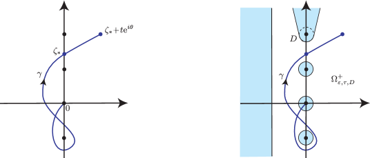
Figure 16: Resurgence of the iterator (Theorem 34.4). Left: A path of analytic continuation for $\hat{\varphi}$. Right: The domain $\Omega^{+}_{{\varepsilon},\tau,D}$ of Lemma 34.6.

Since $\tilde{\varphi}\coloneqq\tilde{v}_{*}-\operatorname{id}$ is given by Lemma 34.2 in the form of the formally convergent series $\sum_{k\geq 0}\tilde{\varphi}_{k}$, the statement can be proved by controlling the formal Borel transforms $\hat{\varphi}_{k}$.

Lemma 34.5.

For each $k\in\mathbb{N}$ we have $\hat{\varphi}_{k}\coloneqq\mathcal{B}(\tilde{\varphi}_{k})\in\hat{\mathscr{R}}_{2\pi{\mathrm{i}}\mathbb{Z}}^{\mathrm{simp}}$.

Lemma 34.6.

Suppose that $0<{\varepsilon}<\pi<\tau$, $0<\kappa\leq 1$ and $D$ is a closed disc of radius ${\varepsilon}$ centred at $2\pi{\mathrm{i}}m$ with $m\in\mathbb{Z}^{*}$, and let

$$\Omega^{+}_{{\varepsilon},\tau,D}\coloneqq\{\,{\zeta}\in\mathbb{C}\mid\mathop{\Re e}\nolimits{\zeta}>-\tau,\;\operatorname{dist}\big{(}{\zeta},2\pi{\mathrm{i}}\mathbb{Z}^{*}\big{)}>{\varepsilon}\,\}\setminus\{\,u{\zeta}\in\mathbb{C}\mid u\in[1,+\infty),\;\pm{\zeta}\in D\,\}$$ (215)

(see Figure 16b). Then there exist $A,M,R>0$ such that, for any naturally parametrised path $\gamma\colon\thinspace[0,\ell]\to\Omega^{+}_{{\varepsilon},\tau,D}$ with

$$s\in[0,{\varepsilon}]\enspace\Longrightarrow\enspace\lvert\gamma(s)\rvert=s,\qquad s>{\varepsilon}\enspace\Longrightarrow\enspace\lvert\gamma(s)\rvert>{\varepsilon},\qquad s\in[0,\ell]\enspace\Longrightarrow\enspace\lvert\gamma(s)\rvert>\kappa s,$$ (216)

one has

$$\left\lvert\operatorname{cont}_{\gamma}\hat{\varphi}_{k}\big{(}\gamma(\ell)\big{)}\right\rvert\leq A\frac{(M\ell)^{k}}{k!}\mathrm{e}^{R\ell}\quad\text{for every $k\geq 0$}.$$ (217)

Lemmas 34.5 and 34.6 imply Theorem 34.4.

According to notation (97), we denote by $\mathbb{D}_{2\pi}$ or $\mathbb{D}_{1}$ the open disc centred at $0$ of radius $2\pi$ or $1$. Lemma 34.6 implies that the series of holomorphic functions $\sum\hat{\varphi}_{k}$ converges normally in any compact subset of $\mathbb{D}_{2\pi}$ (using paths $\gamma$ of the form $[0,{\zeta}]$) and that its sum, which is $\hat{\varphi}$, extends analytically along any naturally parametrised path $\gamma$ which starts as the line segment $[0,1]$ and then stays in $\mathbb{C}\setminus 2\pi{\mathrm{i}}\mathbb{Z}$: indeed, taking ${\varepsilon},\kappa$ small enough and $\tau,m$ large enough, we see that Lemma 34.6 applies to $\gamma$ and the neighbouring paths, so that (217) yields the normal convergence of $\sum_{k\geq 0}\operatorname{cont}_{\gamma}\hat{\varphi}_{k}(\gamma(t)+{\zeta})=\operatorname{cont}_{\gamma}\hat{\varphi}(\gamma(t)+{\zeta})$ for all $t$ and ${\zeta}$ with $\lvert{\zeta}\rvert$ small enough. Therefore $\hat{\varphi}$ is $2\pi{\mathrm{i}}\mathbb{Z}$-resurgent and, combining Lemma 34.5 with the estimates (217), we also get $\hat{\varphi}\in\hat{\mathscr{R}}_{2\pi{\mathrm{i}}\mathbb{Z}}^{\mathrm{simp}}$ by Lemma 30.10.

This establishes $\tilde{v}_{*}\in\tilde{\mathscr{G}}^{\mathrm{simp}}_{0}(2\pi{\mathrm{i}}\mathbb{Z})$, whence $\tilde{u}_{*}\in\tilde{\mathscr{G}}^{\mathrm{simp}}_{0}(2\pi{\mathrm{i}}\mathbb{Z})$ by Theorem 32.2.

For the part of (214) relative to $I^{+}$, we give ourselves an arbitrary $n>1$ and set $\delta_{n}\coloneqq\frac{\pi}{2n}$, $I^{+}_{n}\coloneqq[-\frac{\pi}{2}+\delta_{n},\frac{\pi}{2}-\delta_{n}]$. Given $\gamma$ with endpoint ${\zeta}_{*}\in{\mathrm{i}}\mathbb{R}$, we first replace an initial portion of $\gamma$ with a line segment of length $1$ (unless $\gamma$ stays in $\mathbb{D}_{1}$, in which case the modification of the arguments which follow is trivial) and switch to its natural parametrisation $\gamma\colon\thinspace[0,\ell]\to\mathbb{C}$. We then choose ${\varepsilon}_{n}$ and $\kappa_{n}$ small enough:

$${\varepsilon}_{n} <\min\Big{\{}1,\,\min_{[1,\ell]}\lvert\gamma\rvert,\,\operatorname{dist}\big{(}\gamma\big{(}[0,\ell]\big{)},2\pi{\mathrm{i}}\mathbb{Z}^{*}\big{)},\,\operatorname{dist}\big{(}{\zeta}_{*},2\pi{\mathrm{i}}\mathbb{Z}\big{)}\cos\delta_{n}\Big{\}},$$

$$\kappa_{n} <\min\Big{\{}\min_{[0,\ell]}\tfrac{\lvert\gamma(s)\rvert}{s},\,\min_{t\geq 0}\tfrac{\lvert{\zeta}_{*}+t\,\mathrm{e}^{\pm{\mathrm{i}}\delta_{n}}\rvert}{\ell+t}\Big{\}},$$

and $\tau$ and $m_{n}$ large enough:

$$\tau>-\min\mathop{\Re e}\nolimits\gamma,\qquad m_{n}>\frac{1}{2\pi}\big{(}{\varepsilon}_{n}+\max\lvert\mathop{\Im m}\nolimits\gamma\rvert\big{)},$$

so that Lemma 34.6 applies to the concatenation of paths ${\Gamma}\coloneqq\gamma+[{\zeta}_{*},{\zeta}_{*}+t\,\mathrm{e}^{{\mathrm{i}}{\theta}}]$ for each $t\geq 0$ and ${\theta}\in I^{+}_{n}$; since ${\Gamma}$ has length $\ell+t$, (217) yields

$$\text{$t\geq 0$ and ${\theta}\in I^{+}_{n}$}\quad\Longrightarrow\quad\left\lvert\operatorname{cont}_{\gamma}\hat{\varphi}\big{(}{\zeta}_{*}+t\,\mathrm{e}^{{\mathrm{i}}{\theta}}\big{)}\right\rvert=\left\lvert\operatorname{cont}_{\Gamma}\hat{\varphi}\big{(}{\Gamma}(\ell+t)\big{)}\right\rvert\leq A_{n}\,\mathrm{e}^{(M_{n}+R_{n})(\ell+t)},$$

where $A_{n}$, $M_{n}$ and $R_{n}$ depend on $n$ and $\gamma$ but not on $t$ or ${\theta}$. We thus take

$$\alpha^{+}({\theta})\coloneqq\mathrm{e}^{\ell\beta^{+}({\theta})}\max\big{\{}\,A_{n}\mid\text{$n\geq 1$ s.t.\ ${\theta}\in I^{+}_{n}$}\,\big{\}},\quad\beta^{+}({\theta})\coloneqq\max\big{\{}\,M_{n}+R_{n}\mid\text{$n\geq 1$ s.t.\ ${\theta}\in I^{+}_{n}$}\,\big{\}}$$

for any ${\theta}\in I^{+}$, and get

$$\text{$t\geq 0$ and ${\theta}\in I^{+}$}\quad\Longrightarrow\quad\left\lvert\operatorname{cont}_{\gamma}\hat{\varphi}\big{(}{\zeta}_{*}+t\,\mathrm{e}^{{\mathrm{i}}{\theta}}\big{)}\right\rvert\leq\alpha^{+}({\theta})\,\mathrm{e}^{\beta^{+}({\theta})t}.$$

The part of (214) relative to $I^{-}$ follows from the fact that $\hat{\varphi}^{-}({\zeta})\coloneqq\hat{\varphi}(-{\zeta})$ satisfies all the properties we just obtained for $\hat{\varphi}({\zeta})$, since it is the formal Borel transform of $\tilde{\varphi}^{-}(z)\coloneqq-\tilde{\varphi}(-z)$ which solves the equation $C_{\operatorname{id}-1}\tilde{\varphi}^{-}=C_{\operatorname{id}+b^{-}}\tilde{\varphi}^{-}+b^{-}_{*}$ associated with the simple parabolic germ $f^{-}(z)\coloneqq-f^{-1}(-z)=z+1+b^{-}(z+1)$.

This establishes (214), which yields (in the particular case $\gamma=\{0\}$) $\tilde{v}_{*}\in\tilde{\mathscr{G}}_{0}(I^{+})\cap\tilde{\mathscr{G}}_{0}(I^{-})$, whence $\tilde{u}_{*}\in\tilde{\mathscr{G}}_{0}(I^{+})\cap\tilde{\mathscr{G}}_{0}(I^{-})$ by Theorem 17.3. ∎

Proof of Lemma 34.5.

Since $b(z)\in z^{-2}\mathbb{C}\{{\zeta}\}$, its formal Borel transform is an entire function $\hat{b}({\zeta})$ vanishing at $0$, hence

$$\hat{\varphi}_{0}({\zeta})=\frac{\hat{b}({\zeta})}{\mathrm{e}^{\zeta}-1}\in\hat{\mathscr{R}}_{2\pi{\mathrm{i}}\mathbb{Z}}^{\mathrm{simp}}$$

(cf. Lemma 27.7).

We proceed by induction on $k$ and assume $k\geq 1$ and $\tilde{\varphi}_{k-1}\in\tilde{\mathscr{R}}_{2\pi{\mathrm{i}}\mathbb{Z}}^{\mathrm{simp}}$. By Theorem 30.9 we get $C_{\operatorname{id}+b}\tilde{\varphi}_{k-1}\in\tilde{\mathscr{R}}_{2\pi{\mathrm{i}}\mathbb{Z}}^{\mathrm{simp}}$, thus $B\tilde{\varphi}_{k-1}\in\tilde{\mathscr{R}}_{2\pi{\mathrm{i}}\mathbb{Z}}^{\mathrm{simp}}$, thus (since $\mathcal{B}(B\tilde{\varphi}_{k-1})({\zeta})\in{\zeta}\mathbb{C}\{{\zeta}\}$)

$$\hat{\varphi}_{k}({\zeta})=\frac{1}{\mathrm{e}^{\zeta}-1}\mathcal{B}(B\tilde{\varphi}_{k-1})({\zeta})\in\hat{\mathscr{R}}_{2\pi{\mathrm{i}}\mathbb{Z}},$$

but is it true that all the singularities of all the branches of the analytic continuation of $\hat{\varphi}_{k}$ are simple?

By repeated use of (185), we get

$$\Delta_{\omega_{s}}\cdots\Delta_{\omega_{1}}C_{\operatorname{id}+b}\tilde{\varphi}_{k-1}=\mathrm{e}^{-(\omega_{1}+\cdots+\omega_{s})b}C_{\operatorname{id}+b}\Delta_{\omega_{s}}\cdots\Delta_{\omega_{1}}\tilde{\varphi}_{k-1}$$

for every $s\geq 1$ and $\omega_{1},\ldots,\omega_{s}\in 2\pi{\mathrm{i}}\mathbb{Z}^{*}$, hence

$$\Delta_{\omega_{s}}\cdots\Delta_{\omega_{1}}B\tilde{\varphi}_{k-1}=\text{\boldmath{$B$}}_{\omega_{1},\ldots,\omega_{s}}\Delta_{\omega_{s}}\cdots\Delta_{\omega_{1}}\tilde{\varphi}_{k-1}\quad\text{with}\enspace\text{\boldmath{$B$}}_{\omega_{1},\ldots,\omega_{s}}\coloneqq\mathrm{e}^{-(\omega_{1}+\cdots+\omega_{s})b}C_{\operatorname{id}+b}-\mathop{\hbox{{\rm Id}}}\nolimits.$$

Now, for any $\tilde{\psi}\in\mathbb{C}[[z^{-1}]]$, we have $\text{\boldmath{$B$}}_{\omega_{1},\ldots,\omega_{s}}\tilde{\psi}=\mathrm{e}^{-(\omega_{1}+\cdots+\omega_{s})b}B\tilde{\psi}+(\mathrm{e}^{-(\omega_{1}+\cdots+\omega_{s})b}-1)\tilde{\psi}\in z^{-2}\mathbb{C}[[z^{-1}]]$, thus each of the simple $2\pi{\mathrm{i}}\mathbb{Z}$-resurgent series $\Delta_{\omega_{s}}\cdots\Delta_{\omega_{1}}B\tilde{\varphi}_{k-1}$ has valuation $\geq 2$. By Remark 28.8, the same is true of $\operatorname{\mathcal{A}}^{\gamma}_{\omega}B\tilde{\varphi}_{k-1}$ for every $\omega\in 2\pi{\mathrm{i}}\mathbb{Z}$ and every $\gamma$ starting close to $0$ and ending close to $\omega$: we have

$$\operatorname{cont}_{\gamma}\mathcal{B}(B\tilde{\varphi}_{k-1})(\omega+{\zeta})=\hat{\psi}({\zeta})\frac{\mathrm{Log\hskip 1.5pt}{\zeta}}{2\pi}+R({\zeta})$$

with $\hat{\psi}\in{\zeta}\mathbb{C}\{{\zeta}\}$ and $R\in\mathbb{C}\{{\zeta}\}$ depending on $k$, $\omega$, $\gamma$, hence $\hat{\chi}({\zeta})\coloneqq\frac{\hat{\psi}({\zeta})}{\mathrm{e}^{\zeta}-1}\in\mathbb{C}\{{\zeta}\}$ and (since $\mathrm{e}^{\omega+{\zeta}}\equiv\mathrm{e}^{\zeta}$)

$$\operatorname{cont}_{\gamma}\hat{\varphi}_{k}(\omega+{\zeta})=\frac{c}{2\pi{\mathrm{i}}{\zeta}}+\hat{\chi}({\zeta})\frac{\mathrm{Log\hskip 1.5pt}{\zeta}}{2\pi}+R^{*}({\zeta}),\quad\text{with $c\coloneqq 2\pi{\mathrm{i}}R(0)$ and $R^{*}({\zeta})\in\mathbb{C}\{{\zeta}\}$.}$$

Therefore $\hat{\varphi}_{k}$ has only simple singularities. ∎

Proof of Lemma 34.6.

The set $\Omega^{+}_{{\varepsilon},\tau,D}$ is such that we can find $M_{0},L>0$ so that

$${\zeta}\in\Omega^{+}_{{\varepsilon},\tau,D}\quad\Longrightarrow\quad\left\lvert\frac{{\zeta}}{\mathrm{e}^{\zeta}-1}\right\rvert\leq M_{0}\,\mathrm{e}^{-L\lvert{\zeta}\rvert}.$$ (218)

On the other hand, we can find $C>L$ and $R_{0}>0$ such that the entire function $\hat{b}$ satisfies

$$\lvert\hat{b}({\zeta})\rvert\leq C\lvert{\zeta}\rvert\,\mathrm{e}^{R_{0}\lvert{\zeta}\rvert}\enspace\text{for all ${\zeta}\in\mathbb{C}$, hence}\enspace\lvert\hat{b}^{*k}({\zeta})\rvert\leq C^{k}\frac{\lvert{\zeta}\rvert^{2k-1}}{(2k-1)!}\mathrm{e}^{R_{0}\lvert{\zeta}\rvert}\enspace\text{for all ${\zeta}\in\mathbb{C}$ and $k\in\mathbb{N}^{*}$}$$

by Lemma 13.1.

Let us give ourselves a naturally parametrised path $\gamma\colon\thinspace[0,\ell]\to\Omega^{+}_{{\varepsilon},\tau,D}$ satisfying (216). For any $2\pi{\mathrm{i}}\mathbb{Z}$-resurgent series $\tilde{\psi}$ with formal Borel transform $\hat{\psi}$, we have $B\tilde{\psi}\in\tilde{\mathscr{R}}_{2\pi{\mathrm{i}}\mathbb{Z}}$ by Theorem 22.2, the proof of which shows that $\hat{B}\hat{\psi}\coloneqq\mathcal{B}(B\tilde{\psi})$ can be expressed as an integral transform $\hat{B}\hat{\psi}({\zeta})=\int_{0}^{\zeta}K(\xi,{\zeta})\hat{\psi}(\xi)\,{\mathrm{d}}\xi$ for ${\zeta}$ close to $0$, with kernel function

$$K(\xi,{\zeta})=\sum_{k\geq 1}\frac{(-\xi)^{k}}{k!}\hat{b}^{*k}({\zeta}-\xi).$$

The estimates available for $\hat{b}^{*k}$ show that $K$ is holomorphic in $\mathbb{C}\times\mathbb{C}$, we can thus adapt the arguments of the “easy” Lemma 19.1 and get

$$\operatorname{cont}_{\gamma}\hat{B}\hat{\psi}\big{(}\gamma(s)\big{)}=\int_{0}^{s}K\big{(}\gamma({\sigma}),\gamma(s)\big{)}\operatorname{cont}_{\gamma}\hat{\psi}\big{(}\gamma({\sigma})\big{)}\gamma^{\prime}({\sigma})\,{\mathrm{d}}{\sigma}\quad\text{for all $s\in[0,\ell]$.}$$

The crude estimate

$$\lvert K(\xi,{\zeta})\rvert\leq C\lvert\xi\rvert\,\mathrm{e}^{\frac{C}{\mu}\lvert\xi\rvert+(R_{0}+\mu)\lvert{\zeta}-\xi\rvert}\quad\text{for all $(\xi,{\zeta})\in\mathbb{C}\times\mathbb{C}$,}$$

with arbitrary $\mu>1$, will allow us to bound inductively $\operatorname{cont}_{\gamma}\hat{\varphi}_{k}=\operatorname{cont}_{\gamma}\hat{E}\hat{B}\hat{\varphi}_{k-1}$.

Indeed, the meromorphic function $\hat{\varphi}_{0}=\frac{\hat{b}}{\mathrm{e}^{\zeta}-1}$ satisfies (217) with $A\coloneqq M_{0}C$ and any $R\geq R_{0}$. Suppose now that a $2\pi{\mathrm{i}}\mathbb{Z}$-resurgent function $\hat{\psi}$ satisfies

$$\left\lvert\operatorname{cont}_{\gamma}\hat{\psi}\big{(}\gamma(s)\big{)}\right\rvert\leq\mathrm{e}^{Rs}\Psi(s)\enspace\text{for all $s\in[0,\ell]$,}\qquad\text{with}\enspace R\coloneqq R_{0}+\mu,\enspace\mu\coloneqq\frac{C}{\kappa L},$$

and a certain positive continuous function $\Psi$. Since $\lvert\gamma({\sigma})\rvert\leq{\sigma}$ and $\lvert\gamma(s)-\gamma({\sigma})\rvert\leq s-{\sigma}$, we obtain

$$\left\lvert\operatorname{cont}_{\gamma}\hat{B}\hat{\psi}\big{(}\gamma(s)\big{)}\right\rvert\leq Cs\,\mathrm{e}^{(\frac{C}{\mu}+R)s}\int_{0}^{s}\Psi({\sigma})\,{\mathrm{d}}{\sigma}\enspace\text{for all $s\in[0,\ell]$,}$$

whence $\left\lvert\operatorname{cont}_{\gamma}\hat{E}\hat{B}\hat{\psi}\big{(}\gamma(s)\big{)}\right\rvert\leq M\,\mathrm{e}^{Rs}\int_{0}^{s}\Psi({\sigma})\,{\mathrm{d}}{\sigma}$ with $M\coloneqq\frac{CM_{0}}{\kappa}$ by (218), using $\lvert\gamma(s)\rvert\geq\kappa s$. We thus get $\left\lvert\operatorname{cont}_{\gamma}\hat{\varphi}_{k}\big{(}\gamma(s)\big{)}\right\rvert\leq A\,\mathrm{e}^{Rs}\frac{(Ms)^{k}}{k!}$ by induction on $k$. ∎

35 Fatou coordinates of a simple parabolic germ

35.1  For every $R>0$ and $\delta\in(0,\pi/2)$, we define

$${\Sigma}^{+}_{R,\delta}\coloneqq\{\,r\,\mathrm{e}^{{\mathrm{i}}{\theta}}\in\mathbb{C}\mid r>R,\;\lvert{\theta}\rvert<\pi-\delta\,\},\quad{\Sigma}^{-}_{R,\delta}\coloneqq\{\,r\,\mathrm{e}^{{\mathrm{i}}{\theta}}\in\mathbb{C}\mid r>R,\;\lvert{\theta}-\pi\rvert<\pi-\delta\,\}.$$

Definition 35.1.

A pair of Fatou coordinates at $\infty$ is a pair $(v^{+},v^{-})$ of injective holomorphic maps

$$v^{+}\colon\thinspace{\Sigma}^{+}_{R,\delta}\to\mathbb{C},\qquad v^{-}\colon\thinspace{\Sigma}^{-}_{R,\delta}\to\mathbb{C},$$

with some $R>0$ and $\delta\in(0,\pi/2)$, such that

$$v^{+}\circ f=f_{0}\circ v^{+},\qquad v^{-}\circ f=f_{0}\circ v^{-}.$$

We still assume that $f\in\mathscr{G}_{1}$ has vanishing resiter, with iterator $\tilde{v}_{*}$ and inverse iterator $\tilde{u}_{*}$. We still use the notations $I^{+}=(-\frac{\pi}{2},\frac{\pi}{2})$ and $I^{-}=(\frac{\pi}{2},\frac{3\pi}{2})$.

Theorem 35.2.

There exists locally bounded functions $\beta,\beta_{1}\colon\thinspace I^{+}\cup I^{-}\to(0,+\infty)$ such that $\beta<\beta_{1}$ and

• $\tilde{v}_{*}\in\tilde{\mathscr{G}}_{0}(I^{+},\beta)\cap\tilde{\mathscr{G}}_{0}(I^{-},\beta)$ and $v_{*}^{\pm}\coloneqq\mathscr{S}^{I^{\pm}}\tilde{v}_{*}$ is injective on $\mathscr{D}(I^{\pm},\beta)$ (notation of Definition 9.5);

• $\tilde{u}_{*}\in\tilde{\mathscr{G}}_{0}(I^{+},\beta_{1})\cap\tilde{\mathscr{G}}_{0}(I^{-},\beta_{1})$ and $u_{*}^{\pm}\coloneqq\mathscr{S}^{I^{\pm}}\tilde{u}_{*}$ is injective on $\mathscr{D}(I^{\pm},\beta_{1})$, with

  $$u_{*}^{\pm}\big{(}\mathscr{D}(I^{\pm},\beta_{1})\big{)}\subset\mathscr{D}(I^{\pm},\beta)\quad\text{and}\quad v_{*}^{\pm}\circ u_{*}^{\pm}=\operatorname{id}\enspace\text{on $\mathscr{D}(I^{\pm},\beta_{1})$}.$$

Moreover, the pairs of Fatou coordinates at $\infty$ are the pairs $(v_{*}^{+}+c^{+},v_{*}^{-}+c^{-})$ with arbitrary $c^{+},c^{-}\in\mathbb{C}$.

Remark 35.3.

We may consider $(v_{*}^{+},v_{*}^{-})$ as a normalized pair of Fatou coordinates. Being obtained as Borel sums of a $1$-summable formal diffeomorphism, they admit a $1$-Gevrey asymptotic expansion, and the same is true of the inverse Fatou coordinates $u_{*}^{+}$ and $u_{*}^{-}$. The first use of Borel-Laplace summation for obtaining Fatou coordinates is in [Eca81]. The asymptotic property without the Gevrey qualification can be found in earlier works by G. Birkhoff, G. Szekeres, T. Kimura and J. Écalle—see [Lor05] and [Lod13] for the references; see [LY12] for a recent independent proof and an application to numerical computations.

Proof of Theorem 35.2.

The case $\gamma=\{0\}$ of Theorem 34.4 yields locally bounded functions $\alpha,\beta\colon\thinspace I^{+}\cup I^{-}\to\mathbb{R}^{+}$ such that $\tilde{v}_{*}\in\tilde{\mathscr{G}}_{0}(I^{\pm},\beta,\alpha)$ (notation of Definition 17.1). In view of Theorem 17.3, we can replace $\beta$ by a larger function so that $v_{*}^{\pm}$ is injective on $\mathscr{D}(I^{\pm},\beta)$. We apply again Theorem 17.3: setting

$$\beta\;<\;\beta^{*}\coloneqq\beta+2\sqrt{\alpha}\;<\;\beta_{1}\coloneqq\beta+(1+\sqrt{2})\sqrt{\alpha},$$

we get $\tilde{u}_{*}\in\tilde{\mathscr{G}}_{0}(I^{\pm},\beta^{*})$, hence $\tilde{u}_{*}\in\tilde{\mathscr{G}}_{0}(I^{\pm},\beta_{1})$, and all the desired properties follow.

By Lemma 9.8, we have $f=\mathscr{S}^{I^{\pm}}f$; replacing the above function $\beta$ by a larger one if necessary so as to take into account the domain of definition of $f$, Theorem 17.2 shows that $\mathscr{S}^{I^{\pm}}(\tilde{v}_{*}\circ f)=v_{*}^{\pm}\circ f$ and $\mathscr{S}^{I^{\pm}}(f\circ\tilde{u}_{*})=f\circ u_{*}^{\pm}$. In view of (210) and (213), this yields

$$v_{*}^{\pm}\circ f=f_{0}\circ v_{*}^{\pm},\qquad f\circ u_{*}^{\pm}=u_{*}^{\pm}\circ f_{0}.$$ (219)

We see that for any $\delta\in(0,\pi/2)$ there exists $R>0$ such that ${\Sigma}^{\pm}_{R,\delta}\subset\mathscr{D}(I^{\pm},\beta)$, therefore $(v_{*}^{+},v_{*}^{-})$ is a pair of Fatou coordinates.

Suppose now that $v^{\pm}$ is holomorphic and injective on ${\Sigma}^{\pm}_{R,\delta}$. Replacing the above function $\beta$ by a larger one if necessary, we may suppose $\beta\geq R$, then $\mathscr{D}(J^{\pm},\beta)\subset{\Sigma}^{\pm}_{R,\delta}$ with $J^{+}\coloneqq(-\frac{\pi}{2}+\delta,\frac{\pi}{2}-\delta)$, $J^{-}\coloneqq(\frac{\pi}{2}+\delta,\frac{3\pi}{2}-\delta)$. By Theorem 17.3, we have $u_{*}^{\pm}\big{(}\mathscr{D}(J^{\pm},\beta_{1})\big{)}\subset\mathscr{D}(J^{\pm},\beta)$, thus $\Phi^{\pm}\coloneqq v^{\pm}\circ u_{*}^{\pm}$ is holomorphic and injective on $\mathscr{D}(J^{\pm},\beta_{1})$. In view of (219), the equation $v^{\pm}\circ f=f_{0}\circ v^{\pm}$ is equivalent to $f_{0}\circ\Phi^{\pm}=\Phi^{\pm}\circ f_{0}$, i.e. $\Phi^{\pm}=\operatorname{id}+\Psi^{\pm}$ with $\Psi^{\pm}$ $1$-periodic. If $\Psi^{\pm}$ is a constant $c^{\pm}$, then we find $v^{\pm}=v_{*}^{\pm}+c^{\pm}$. In general, the periodicity of $\Psi^{\pm}$ allows one to extend analytically $\Phi^{\pm}$ to the whole of $\mathbb{C}$ and we get an injective entire function; the Casorati-Weierstrass theorem shows that such a function must be of the form $az+c$, hence $\Psi^{\pm}$ is constant. ∎

35.2  Here are a few dynamical consequences of Theorem 35.2. The domain $\mathscr{D}^{+}\coloneqq\mathscr{D}(I^{+},\beta_{1})$ is invariant by the normal form $f_{0}=\operatorname{id}+1$, while $\mathscr{D}^{-}\coloneqq\mathscr{D}(I^{-},\beta_{1})$ is invariant by the backward dynamics $f_{0}^{\circ(-1)}=\operatorname{id}-1$, hence

$$\mathscr{P}^{+}\coloneqq u_{*}^{+}(\mathscr{D}^{+})\;\text{ is invariant by~{}$f$,}\quad\mathscr{P}^{-}\coloneqq u_{*}^{-}(\mathscr{D}^{-})\;\text{ is invariant by~{}$f^{\circ(-1)}$,}$$ (220)

and the conjugacy relations $f=u_{*}^{+}\circ f_{0}\circ v_{*}^{+}$, $f^{\circ(-1)}=u_{*}^{-}\circ f_{0}^{\circ(-1)}\circ v_{*}^{-}$ yield

$$z\in\mathscr{P}^{+}\enspace\Longrightarrow\enspace f^{\circ n}(z)=u_{*}^{+}\big{(}v_{*}^{+}(z)+n\big{)},\qquad z\in\mathscr{P}^{-}\enspace\Longrightarrow\enspace f^{\circ(-n)}(z)=u_{*}^{-}\big{(}v_{*}^{-}(z)-n\big{)}$$

for every $n\in\mathbb{N}$. We thus see that all the forward orbits of $f$ which start in $\mathscr{P}^{+}$ and all the backward orbits of $f$ which start in $\mathscr{P}^{-}$ are infinite and converge to the fixed point at $\infty$ (we could even describe the asymptotics with respect to the discrete time $n$)—see Figure 17.

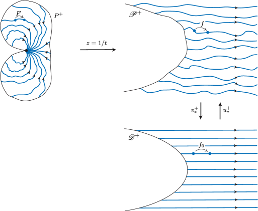
Figure 17: The dynamics in the attracting petal viewed in three coordinates.

All this can be transferred to the variable $t=1/z$ and we get for the dynamics of $F$ a version of what is usually called the “Leau-Fatou flower theorem”: we define the attracting and repelling “petals” by

$$P^{+}\coloneqq\{\,t\in\mathbb{C}^{*}\mid 1/t\in\mathscr{P}^{+}\,\},\qquad P^{-}\coloneqq\{\,t\in\mathbb{C}^{*}\mid 1/t\in\mathscr{P}^{-}\,\},$$

whose union is a punctured neighbourhood of $0$, and we see that all the forward orbits of $F$ which start in $P^{+}$ and all the backward orbits of $F$ which start in $P^{-}$ are infinite and converge to $0$ (see Figure 17). Notice that $P^{+}$ and $P^{-}$ overlap, giving rise to two families of bi-infinite orbits which are positively and negatively asymptotic to the fixed point.

We can also define Fatou coordinates and inverse Fatou coordinates at $0$ as well as their formal counterparts by

$$V_{*}^{\pm}(t)\coloneqq v_{*}^{\pm}(1/t),\quad U_{*}^{\pm}(z)\coloneqq 1/u_{*}^{\pm}(z),\qquad\tilde{V}_{*}(t)\coloneqq\tilde{v}_{*}(1/t),\quad\tilde{U}_{*}(z)\coloneqq 1/\tilde{u}_{*}(z),$$

so that

$$t\in P^{+} \Rightarrow V_{*}^{+}\big{(}F(t)\big{)}=V_{*}^{+}(t)+1, \quad z\in\mathscr{D}^{+} \Rightarrow F\big{(}U_{*}^{+}(z)\big{)}=U_{*}^{+}(z+1),$$ (221)

$$t\in P^{-} \Rightarrow V_{*}^{-}\big{(}F^{\circ(-1)}(t)\big{)}=V_{*}^{-}(t)-1, \quad z\in\mathscr{D}^{-} \Rightarrow F^{\circ(-1)}\big{(}U_{*}^{-}(z)\big{)}=U_{*}^{-}(z-1).$$ (222)

Observe that, with the notation $\tilde{v}_{*}(z)=z+\sum_{k\geq 1}a_{k}z^{-k}$, we have

$$V_{*}^{\pm}(t)\sim\tilde{V}_{*}(t)=\frac{1}{t}+\sum_{k\geq 1}a_{k}t^{k},$$

whereas $\tilde{u}_{*}(z)=z+\tilde{\psi}(z)$ with $\tilde{\psi}(z)=\sum_{k\geq 1}b_{k}z^{-k}\in z^{-1}\mathbb{C}[[z^{-1}]]$ implies

$$\tilde{U}_{*}(z)=z^{-1}\big{(}1+z^{-1}\tilde{\psi}(z)\big{)}^{-1}\in z^{-1}\mathbb{C}[[z^{-1}]].$$

By Theorems 13.3 and 30.9, we see that $\tilde{U}_{*}$ is a simple $2\pi{\mathrm{i}}\mathbb{Z}$-resurgent series, which is $1$-summable in the directions of $I^{+}$ and $I^{-}$, with

$$U_{*}^{\pm}=\mathscr{S}^{I^{\pm}}\tilde{U}_{*}.$$

35.3  Of course it may happen that one of the formal series $\tilde{v}_{*}$, $\tilde{u}_{*}$, $\tilde{V}_{*}$, $\tilde{U}_{*}$ and thus all of them be convergent. But this is the exception rather than the rule.

There is a case in which one easily proves that all of them are divergent.

Lemma 35.4.

If $F(t)$ or $F^{\circ(-1)}(t)$ extends to an entire function, then the formal series $\tilde{v}_{*}$, $\tilde{u}_{*}$, $\tilde{V}_{*}$, $\tilde{U}_{*}$ are divergent.

Proof.

Suppose that $F$ is entire. The function $U_{*}^{-}(z)$, intially defined and holomorphic in $\mathscr{D}^{-}$, which contains a left half-plane $\{\mathop{\Re e}\nolimits z<-c\}$, can be analytically continued by repeated use of (222): for any $n\in\mathbb{N}^{*}$, the formula

$$U_{*}^{-}(z)=F\big{(}U_{*}^{-}(z-1)\big{)}=\cdots=F^{\circ n}\big{(}U_{*}^{-}(z-n)\big{)}$$

yields its analytic continuation in $\{\mathop{\Re e}\nolimits(z)<-c+n\}$, hence $U_{*}^{-}$ extends to an entire function. If $\tilde{U}_{*}$ had positive radius of convergence, then we would get $U_{*}^{-}\sim_{1}\tilde{U}_{*}$ in a full neighbourhood of $\infty$ by Lemma 9.8, in particular $U_{*}^{-}(z)$ would tend to $0$ as $\lvert z\rvert\to\infty$ and thus be uniformly bounded; then the entire function $U_{*}^{-}$ would be constant by Liouville’s theorem, which is impossible because $\tilde{U}_{*}(z)=z^{-1}+O(z^{-2})$.

If it is $F^{\circ(-1)}$ that extends to an entire function, then $U_{*}^{+}$ extends to an entire function by virtue of (221) and one can argue similarly to prove that $\tilde{U}_{*}$ is divergent. ∎

36 The horn maps and the analytic classification

In (220) we have defined $\mathscr{P}^{+}$ and $\mathscr{P}^{-}$ so that $v_{*}^{+}$ induces a biholomorphism $\mathscr{P}^{+}\xrightarrow{\sim}\mathscr{D}^{+}$ and $u_{*}^{-}$ induces a biholomorphism $\mathscr{D}^{-}\xrightarrow{\sim}\mathscr{P}^{-}$. We can thus define a holomorphic function

$$h\coloneqq v_{*}^{+}\circ u_{*}^{-}\colon\thinspace\mathscr{D}^{-}\cap(u_{*}^{-})^{-1}(\mathscr{P}^{+})\to\mathscr{D}^{+}\cap v_{*}^{+}(\mathscr{P}^{-}),\quad\text{such that}\enspace h\circ f_{0}=f_{0}\circ h$$ (223)

(the fact that $h$ conjugates $f_{0}$ with itself stems from (219)).

Let us define, for any $R>0$ and $\delta\in(0,\pi/2)$,

$$\mathscr{V}^{\textnormal{up}}_{R,\delta}\coloneqq\{\,r\,\mathrm{e}^{{\mathrm{i}}{\theta}}\mid r>R,\;\delta<{\theta}<\pi-\delta\,\},\quad\mathscr{V}^{\textnormal{low}}_{R,\delta}\coloneqq\{\,r\,\mathrm{e}^{{\mathrm{i}}{\theta}}\mid r>R,\;\pi+\delta<{\theta}<2\pi-\delta\,\}.$$

Since $v_{*}^{+}$ and $u_{*}^{-}$ are close to identity near $\infty$, there exists $R>0$ such that the domain of definition of $h$ has a connected component which contains $\mathscr{V}^{\textnormal{up}}_{R,\pi/4}$ and a connected component which contains $\mathscr{V}^{\textnormal{low}}_{R,\pi/4}$, so that in fact formula (223) defines a function $h^{\textnormal{up}}$ and a function $h^{\textnormal{low}}$.

Lemma 36.1.

There exists ${\sigma}>0$ such that the function $h^{\textnormal{up}}$ extends analytically to the upper half-plane $\{\mathop{\Im m}\nolimits z>{\sigma}\}$ and the function $h^{\textnormal{low}}$ extends analytically to the lower half-plane $\{\mathop{\Im m}\nolimits z<-{\sigma}\}$. The functions $h^{\textnormal{up}}-\operatorname{id}$ and $h^{\textnormal{low}}-\operatorname{id}$ are $1$-periodic and admit convergent Fourier expansions

$$h_{*}^{\textnormal{up}}(z)-z=\sum_{m=1}^{+\infty}A_{-m}\mathrm{e}^{2\pi{\mathrm{i}}mz},\qquad h_{*}^{\textnormal{low}}(z)-z=\sum_{m=1}^{+\infty}A_{m}\mathrm{e}^{-2\pi{\mathrm{i}}mz},$$ (224)

with $A_{m}=O(\mathrm{e}^{\lambda\lvert m\rvert})$ for every $\lambda>2\pi{\sigma}$.

Proof.

The conjugacy relation $h^{\textnormal{up/low}}\circ f_{0}=f_{0}\circ h^{\textnormal{up/low}}$ implies that $h^{\textnormal{up/low}}$ is of the form $\operatorname{id}+P^{\textnormal{up/low}}$ with a $1$-periodic holomorphic function $P^{\textnormal{up/low}}\colon\thinspace\mathscr{V}^{\textnormal{up/low}}_{R,\pi/4}\to\mathbb{C}$. By $1$-periodicity, $P^{\textnormal{up/low}}$ extends analytically to an upper/lower half-plane and can be written as $\chi(\mathrm{e}^{\pm 2\pi{\mathrm{i}}z})$, with $\chi$ holomorphic in the punctured disc $\mathbb{D}^{*}_{2\pi{\sigma}}$. The asymptotic behaviour of $v_{*}^{+}$ and $u_{*}^{-}$ at $\infty$ in $\mathscr{D}\big{(}(-\frac{\pi}{4},\frac{\pi}{4}),\beta_{1}\big{)}$ shows that $h^{\textnormal{up/low}}(z)=z+o(1)$, hence $\chi(Z)\xrightarrow[Z\to 0]{}0$. Thus $\chi$ is holomorphic in $\mathbb{D}_{2\pi{\sigma}}$ and vanishes at $0$; its Taylor expansions yields the Fourier series of $P^{\textnormal{up/low}}$. ∎

Definition 36.2.

We call $(h^{\textnormal{up}},h^{\textnormal{low}})$ the pair of lifted horn maps of $f$. We call the coefficients of the sequence $(A_{m})_{m\in\mathbb{Z}^{*}}$ the Écalle-Voronin invariants of $f$.

Theorem 36.3.

Two simple parabolic germs at $\infty$ with vanishing resiter, $f$ and $g$, are analytically conjugate if and only if there exists $c\in\mathbb{C}$ such that their pairs of lifted horn maps $(h_{f}^{\textnormal{up}},h_{f}^{\textnormal{low}})$ and $(h_{g}^{\textnormal{up}},h_{g}^{\textnormal{low}})$ are related by

$$h_{g}^{\textnormal{up}}(z)\equiv h_{f}^{\textnormal{up}}(z+c)-c,\qquad h_{g}^{\textnormal{low}}(z)\equiv h_{f}^{\textnormal{low}}(z+c)-c,$$ (225)

or, equivalently,

$$A_{m}(g)=\mathrm{e}^{-2\pi{\mathrm{i}}mc}A_{m}(f)\quad\text{for every $m\in\mathbb{Z}^{*}$.}$$ (226)

Proof.

We denote by $\tilde{v}_{f}$, $v_{f}^{\pm}$, $\tilde{u}_{f}$, $u_{f}^{\pm}$ the iterator of $f$, its Borel sums and their inverses, and similarly $\tilde{v}_{g}$, $v_{g}^{\pm}$, $\tilde{u}_{g}$, $u_{g}^{\pm}$ for $g$.

Suppose that $f$ and $g$ are analytically conjugate, so there exists $h\in\mathscr{G}$ (convergent!) such that $g\circ h=h\circ f$. It follows that $\tilde{v}_{f}\circ h^{\circ(-1)}\circ g=f_{0}\circ\tilde{v}_{f}\circ h^{\circ(-1)}$, hence there exists $c\in\mathbb{C}$ such that $\tilde{v}_{f}\circ h^{\circ(-1)}=\tilde{v}_{g}+c$ by Lemma 34.2. Let $\tau\coloneqq\operatorname{id}+c$. We have $\tilde{v}_{g}=\tau^{-1}\circ\tilde{v}_{f}\circ h^{\circ(-1)}$ and $\tilde{u}_{g}=h\circ\tilde{u}_{f}\circ\tau$, whence $v_{g}^{+}=\tau^{-1}\circ v_{f}^{+}\circ h^{\circ(-1)}$ and $u_{g}^{-}=h\circ u_{f}^{-}\circ\tau$ by Theorem 17.2 and Lemma 9.8. This implies $v_{g}^{+}\circ u_{g}^{-}=\tau^{-1}\circ v_{f}^{+}\circ u_{f}^{-}\circ\tau$, i.e. $h_{g}^{\textnormal{up/low}}=\tau^{-1}\circ h_{f}^{\textnormal{up/low}}\circ\tau$, as desired.

Suppose now that there exists $c\in\mathbb{C}$ satisfying (225). We rewrite this relation as

$$h_{g}^{\textnormal{up}}=\tau^{-1}\circ h_{f}^{\textnormal{up}}\circ\tau,\qquad h_{g}^{\textnormal{low}}=\tau^{-1}\circ h_{f}^{\textnormal{low}}\circ\tau,$$

with $\tau=\operatorname{id}+c$. This implies

$$\tau\circ v_{g}^{+}\circ u_{g}^{-}=v_{f}^{+}\circ u_{f}^{-}\circ\tau\quad\text{on $\mathscr{V}_{R,\delta}^{\textnormal{up}}\cup\mathscr{V}_{R,\delta}^{\textnormal{low}}$}$$

with, say, $\delta=3\pi/4$ and $R$ large enough. Therefore

$$u_{f}^{+}\circ\tau\circ v_{g}^{+}=u_{f}^{-}\circ\tau\circ v_{g}^{-}\quad\text{on $\mathscr{V}_{R^{\prime},\pi/4}^{\textnormal{up}}\cup\mathscr{V}_{R^{\prime},\pi/4}^{\textnormal{low}}$}.$$

This indicates that the functions $u_{f}^{+}\circ\tau\circ v_{g}^{+}$ and $u_{f}^{-}\circ\tau\circ v_{g}^{-}$ can be glued to form a function $h$ holomorphic in punctured neighbourhood of $\infty$; the asymptotic behaviour then shows that $h$ is holomorphic at $\infty$, with Taylor series $\tilde{u}_{f}\circ\tau\circ\tilde{v}_{g}$. The conjugacy relations $\tilde{u}_{g}=g\circ\tilde{u}_{g}\circ f_{0}^{\circ(-1)}$ and $\tau\circ\tilde{v}_{f}\circ f=f_{0}\circ\tau\circ\tilde{v}_{f}$ imply $\tilde{u}_{g}\circ\tau\circ\tilde{v}_{f}\circ f=g\circ\tilde{u}_{g}\circ\tau\circ\tilde{v}_{f}$, hence $f$ and $g$ are analytically conjugate by $h$. ∎

Theorem 36.3 is just one part of Écalle-Voronin’s classification result in the case of simple parabolic germs with vanishing resiter. The other part of the result (more difficult) says that any pair of Fourier series of the form $\big{(}\sum_{m\geq 1}A_{-m}\mathrm{e}^{2\pi{\mathrm{i}}mz},\sum_{m\geq 1}A_{m}\mathrm{e}^{-2\pi{\mathrm{i}}mz}\big{)}$, where the first (resp. second) one is holomorphic in an upper (resp. lower) half-plane, can be obtained as $(h_{*}^{\textnormal{up}}-\operatorname{id},h_{*}^{\textnormal{low}}-\operatorname{id})$ for a simple parabolic germ $f$ with vanishing resiter.

37 The Bridge Equation and the action of the symbolic Stokes automorphism

37.1  Let us give ourselves a simple parabolic germ at $\infty$ with vanishing resiter, $f$. So far, we have only exploited the summability statement contained in Theorem 35.2 and we have see that a deep information on the analytic conjugacy class of $f$ is encoded by the discrepancy between the Borel sums $v_{*}^{+}$ and $v_{*}^{-}$, i.e. by the lifted horn maps. Let us now see how the analysis of this discrepancy lends itself to alien calculus, i.e. to the study of the singularities in the Borel plane.

We first use the operators $\Delta_{\omega}$ of Sections 28–30 with $\omega\in 2\pi{\mathrm{i}}\mathbb{Z}^{*}$. They are derivations of the algebra $\tilde{\mathscr{R}}_{2\pi{\mathrm{i}}\mathbb{Z}}^{\mathrm{simp}}$, and they induce operators $\Delta_{\omega}\colon\thinspace\tilde{\mathscr{G}}_{2\pi{\mathrm{i}}\mathbb{Z}}^{\mathrm{simp}}\to\tilde{\mathscr{R}}_{2\pi{\mathrm{i}}\mathbb{Z}}^{\mathrm{simp}}$ defined by $\Delta_{\omega}(\operatorname{id}+\tilde{\varphi})\equiv\Delta_{\omega}\tilde{\varphi}$.

Theorem 37.1.

There exists a sequence of complex numbers $(C_{\omega})_{\omega\in 2\pi{\mathrm{i}}\mathbb{Z}^{*}}$ such that

$$\Delta_{\omega}\tilde{u}_{*}=C_{\omega}\partial\tilde{u}_{*},\qquad\Delta_{\omega}\tilde{v}_{*}=-C_{\omega}\,\mathrm{e}^{-\omega(\tilde{v}_{*}-\operatorname{id})}$$ (227)

for each $\omega\in 2\pi{\mathrm{i}}\mathbb{Z}^{*}$.

Proof.

Let us apply $\Delta_{\omega}$ to both sides of the conjugacy equation (213): by Theorem 32.2, since $\Delta_{\omega}f$ and $\Delta_{\omega}f_{0}$ vanish, we get

$$(\partial f)\circ\tilde{u}_{*}\cdot\Delta_{\omega}\tilde{u}_{*}=(\Delta_{\omega}\tilde{u}_{*})\circ f_{0}$$

(we also used the fact that $\mathrm{e}^{-\omega(f_{0}-\operatorname{id})}=1$, since $\omega\in 2\pi{\mathrm{i}}\mathbb{Z}^{*}$). By applying $\partial$ to (213), we also get

$$(\partial f)\circ\tilde{u}_{*}\cdot\partial\tilde{u}_{*}=(\partial\tilde{u}_{*})\circ f_{0}.$$

Since $\partial\tilde{u}_{*}=1+O(z^{-2})$, this implies that the formal series $\tilde{C}\coloneqq\frac{\Delta_{\omega}\tilde{u}_{*}}{\partial\tilde{u}_{*}}\in\mathbb{C}[[z^{-1}]]$ satisfies $\tilde{C}=\tilde{C}\circ f_{0}$. Writing $\tilde{C}\circ f_{0}-\tilde{C}=\partial\tilde{C}+\frac{1}{2!}\partial^{2}\tilde{C}+\cdots$ and reasoning on the valuation of $\partial\tilde{C}$, we see that $\tilde{C}$ must be constant.

We have $(\Delta_{\omega}\tilde{u}_{*})\circ\tilde{v}_{*}\cdot\partial\tilde{v}_{*}=\tilde{C}(\partial\tilde{u}_{*})\circ\tilde{v}_{*}\cdot\partial\tilde{v}_{*}=\tilde{C}\,\partial(\tilde{u}_{*}\circ\tilde{v}_{*})=\tilde{C}$, hence Formula (207) yields $\Delta_{\omega}\tilde{v}=-\tilde{C}\,\mathrm{e}^{-\omega(\tilde{v}_{*}-\operatorname{id})}$. ∎

The first equation in (227) is called “the Bridge Equation for simple parabolic germs”: like Equation (203), it yields a bridge between ordinary differential calculus (here involving $\partial$) and alien calculus (when dealing with the solution $\tilde{u}$ of the conjugacy equation (213)).

37.2  From the operators $\Delta_{\omega}$ we can go the operators $\Delta_{\omega}^{+}$ by means of formula (142) of Theorem 29.1, according to which, if one sets $\Omega\coloneqq 2\pi{\mathrm{i}}\mathbb{N}^{*}$ or $\Omega\coloneqq-2\pi{\mathrm{i}}\mathbb{N}^{*}$, then

$$\Delta^{+}_{\omega}=\sum_{s\geq 1}\tfrac{1}{s!}\sum_{\begin{subarray}{c}\omega_{1},\ldots,\omega_{s}\in\Omega\\ \omega_{1}+\cdots+\omega_{s}=\omega\end{subarray}}\Delta_{\omega_{s}}\circ\cdots\circ\Delta_{\omega_{2}}\circ\Delta_{\omega_{1}}\quad\text{for $\omega\in\Omega$.}$$ (228)

We also define

$$\Delta^{-}_{\omega}\coloneqq\sum_{s\geq 1}\tfrac{(-1)^{s}}{s!}\sum_{\begin{subarray}{c}\omega_{1},\ldots,\omega_{s}\in\Omega\\ \omega_{1}+\cdots+\omega_{s}=\omega\end{subarray}}\Delta_{\omega_{s}}\circ\cdots\circ\Delta_{\omega_{2}}\circ\Delta_{\omega_{1}}\quad\text{for $\omega\in\Omega$.}$$ (229)

The latter family of operators is related to Exercise 29.1: they correspond to the homogeneous components of $\exp(-{\Delta\raisebox{1.72218pt}{$\scriptscriptstyle/$}\hskip 3.00003pt_{{\mathrm{i}}\mathbb{R}^{\pm}}})$ the same way the operators $\Delta^{+}_{\omega}$ correspond to the homogeneous components of $\exp({\Delta\raisebox{1.72218pt}{$\scriptscriptstyle/$}\hskip 3.00003pt_{{\mathrm{i}}\mathbb{R}^{\pm}}})$—see formulas (165)–(232).

Corollary 37.2.

Let $\Omega\coloneqq 2\pi{\mathrm{i}}\mathbb{N}^{*}$ or $\Omega\coloneqq-2\pi{\mathrm{i}}\mathbb{N}^{*}$. For each $\omega\in\Omega$, define

$$S^{+}_{\omega}\coloneqq-\sum_{s\geq 1}\tfrac{1}{s!}\sum_{\begin{subarray}{c}\omega_{1},\ldots,\omega_{s}\in\Omega\\ \omega_{1}+\cdots+\omega_{s}=\omega\end{subarray}}{\Gamma}_{\omega_{1},\ldots,\omega_{s}}C_{\omega_{1}}\cdots C_{\omega_{s}},\quad S^{-}_{\omega}\coloneqq\sum_{s\geq 1}\tfrac{(-1)^{s-1}}{s!}\sum_{\begin{subarray}{c}\omega_{1},\ldots,\omega_{s}\in\Omega\\ \omega_{1}+\cdots+\omega_{s}=\omega\end{subarray}}{\Gamma}_{\omega_{1},\ldots,\omega_{s}}C_{\omega_{1}}\cdots C_{\omega_{s}}$$

with ${\Gamma}_{\omega_{1}}\coloneqq 1$ and ${\Gamma}_{\omega_{1},\ldots,\omega_{s}}\coloneqq\omega_{1}(\omega_{1}+\omega_{2})\cdots(\omega_{1}+\cdots+\omega_{s-1})$. Then

$$\Delta^{+}_{\omega}\tilde{v}_{*}=S^{+}_{\omega}\,\mathrm{e}^{-\omega(\tilde{v}_{*}-\operatorname{id})},\qquad\Delta^{-}_{\omega}\tilde{v}_{*}=S^{-}_{\omega}\,\mathrm{e}^{-\omega(\tilde{v}_{*}-\operatorname{id})}.$$ (230)

Proof.

Let $\tilde{\varphi}\coloneqq\tilde{v}_{*}-\operatorname{id}$, so that the second equation in (227) reads $\Delta_{\omega}\tilde{\varphi}=-C_{\omega}\,\mathrm{e}^{-\omega\tilde{\varphi}}$. By repeated use of formula (186) of Theorem 30.9, we get $\Delta_{\omega_{2}}\Delta_{\omega_{1}}\tilde{\varphi}=\omega_{1}C_{\omega_{1}}\,\mathrm{e}^{-\omega_{1}\tilde{\varphi}}\Delta_{\omega_{2}}\tilde{\varphi}=-\omega_{1}C_{\omega_{1}}C_{\omega_{2}}\,\mathrm{e}^{-(\omega_{1}+\omega_{2})\tilde{\varphi}}$, $\Delta_{\omega_{3}}\Delta_{\omega_{2}}\Delta_{\omega_{1}}\tilde{\varphi}=\ldots\,$, etc. The general formula is

$$\Delta_{\omega_{s}}\cdots\Delta_{\omega_{1}}\tilde{\varphi}=-{\Gamma}_{\omega_{1},\ldots,\omega_{s}}C_{\omega_{1}}\cdots C_{\omega_{s}}\,\mathrm{e}^{-(\omega_{1}+\cdots+\omega_{s})\tilde{\varphi}},$$

whence the conclusion follows with the help of (228)–(229). ∎

In fact, in view of Remark 28.8, the above proof shows that, for every $\omega\in 2\pi{\mathrm{i}}\mathbb{Z}$ and for every path $\gamma$ which starts close to $0$ and ends close to $\omega$, there exists $S_{\omega}^{\gamma}\in\mathbb{C}$ such that $\operatorname{\mathcal{A}}_{\omega}^{\gamma}\tilde{v}_{*}=S_{\omega}^{\gamma}\,\mathrm{e}^{-\omega(\tilde{v}_{*}-\operatorname{id})}$.

37.3  We now wish to compute the action of the symbolic Stokes automorphism ${\Delta\raisebox{1.72218pt}{$\scriptscriptstyle/$}\hskip 3.00003pt^{+}_{{\mathrm{i}}\mathbb{R}^{\pm}}}$ on $\tilde{v}_{*}$ and to describe the Stokes phenomenon in the spirit of Section 29.3, so as to recover the horn maps of Section 36. We shall make use of the spaces

$$\tilde{E}^{\pm}\coloneqq\tilde{E}(2\pi{\mathrm{i}}\mathbb{Z},{\mathrm{i}}\mathbb{R}^{\pm})=\stackrel{{\scriptstyle\raisebox{-0.60275pt}{$\scriptscriptstyle\wedge$}}}{{\displaystyle\bigoplus_{\omega\in\pm 2\pi{\mathrm{i}}\mathbb{N}}}}\mathrm{e}^{-\omega z}\tilde{\mathscr{R}}_{2\pi{\mathrm{i}}\mathbb{Z}}^{\mathrm{simp}}$$

introduced in Section 29.4; since $2\pi{\mathrm{i}}\mathbb{Z}$ is an additive subgroup of $\mathbb{C}$, these spaces are differential algebras,

$$\tilde{E}^{+}=\tilde{\mathscr{R}}_{2\pi{\mathrm{i}}\mathbb{Z}}^{\mathrm{simp}}[[\mathrm{e}^{-2\pi{\mathrm{i}}z}]],\qquad\tilde{E}^{-}=\tilde{\mathscr{R}}_{2\pi{\mathrm{i}}\mathbb{Z}}^{\mathrm{simp}}[[\mathrm{e}^{2\pi{\mathrm{i}}z}]],\qquad\partial=\frac{{\mathrm{d}}\,}{{\mathrm{d}}z},$$

on which are defined the directional alien derivation ${\Delta\raisebox{1.72218pt}{$\scriptscriptstyle/$}\hskip 3.00003pt_{{\mathrm{i}}\mathbb{R}^{\pm}}}$ and the symbolic Stokes automorphism ${\Delta\raisebox{1.72218pt}{$\scriptscriptstyle/$}\hskip 3.00003pt^{+}_{{\mathrm{i}}\mathbb{R}^{\pm}}}=\exp({\Delta\raisebox{1.72218pt}{$\scriptscriptstyle/$}\hskip 3.00003pt_{{\mathrm{i}}\mathbb{R}^{\pm}}})$. According to Remark 29.6, both operators commute with the differential $\partial$. So does the “inverse symbolic Stokes automorphism” ${\Delta\raisebox{1.72218pt}{$\scriptscriptstyle/$}\hskip 3.00003pt^{-}_{{\mathrm{i}}\mathbb{R}^{\pm}}}\coloneqq\exp(-{\Delta\raisebox{1.72218pt}{$\scriptscriptstyle/$}\hskip 3.00003pt_{{\mathrm{i}}\mathbb{R}^{\pm}}})$.

We find it convenient to modify slightly the notation for their homogeneous components: from now on, we set

$$\omega\in 2\pi{\mathrm{i}}\mathbb{Z},\enspace m\in\mathbb{Z},\enspace\tilde{\varphi}\in\tilde{\mathscr{R}}_{2\pi{\mathrm{i}}\mathbb{Z}}^{\mathrm{simp}}\quad\Longrightarrow\quad\left\{\begin{aligned} \raisebox{0.99025pt}{ {$\stackrel{{\scriptstyle\raisebox{-0.69318pt}{$\scriptscriptstyle\bullet$}}}{{\Delta}}_{\raisebox{-0.69318pt}[3.01389pt][0.0pt]{$\scriptstyle\omega$}}$}}(\mathrm{e}^{-2\pi{\mathrm{i}}mz}\tilde{\varphi})&\coloneqq\mathrm{e}^{-(2\pi{\mathrm{i}}m+\omega)z}\Delta_{\omega}\tilde{\varphi},\\[4.30554pt] \raisebox{0.99025pt}{ {$\stackrel{{\scriptstyle\raisebox{-0.69318pt}{$\scriptscriptstyle\bullet$}}}{{\Delta}}_{\raisebox{-0.69318pt}{$\scriptstyle\omega$}}^{\raisebox{-2.56181pt}{$\scriptstyle\pm$}}$}}(\mathrm{e}^{-2\pi{\mathrm{i}}mz}\tilde{\varphi})&\coloneqq\mathrm{e}^{-(2\pi{\mathrm{i}}m+\omega)z}\Delta^{\pm}_{\omega}\tilde{\varphi},\end{aligned}\right.$$ (231)

so that

$${\Delta\raisebox{1.72218pt}{$\scriptscriptstyle/$}\hskip 3.00003pt_{{\mathrm{i}}\mathbb{R}^{+}}} =\sum_{\omega\in 2\pi{\mathrm{i}}\mathbb{N}^{*}}\raisebox{0.99025pt}{ {$\stackrel{{\scriptstyle\raisebox{-0.69318pt}{$\scriptscriptstyle\bullet$}}}{{\Delta}}_{\raisebox{-0.69318pt}[3.01389pt][0.0pt]{$\scriptstyle\omega$}}$}}\quad\text{on $\tilde{E}^{+}$,} {\Delta\raisebox{1.72218pt}{$\scriptscriptstyle/$}\hskip 3.00003pt_{{\mathrm{i}}\mathbb{R}^{-}}} =\sum_{\omega\in-2\pi{\mathrm{i}}\mathbb{N}^{*}}\raisebox{0.99025pt}{ {$\stackrel{{\scriptstyle\raisebox{-0.69318pt}{$\scriptscriptstyle\bullet$}}}{{\Delta}}_{\raisebox{-0.69318pt}[3.01389pt][0.0pt]{$\scriptstyle\omega$}}$}}\quad\text{on $\tilde{E}^{-}$,}$$

$${\Delta\raisebox{1.72218pt}{$\scriptscriptstyle/$}\hskip 3.00003pt^{\pm}_{{\mathrm{i}}\mathbb{R}^{+}}} =\exp(\pm{\Delta\raisebox{1.72218pt}{$\scriptscriptstyle/$}\hskip 3.00003pt_{{\mathrm{i}}\mathbb{R}^{+}}})=\mathop{\hbox{{\rm Id}}}\nolimits+\sum_{\omega\in 2\pi{\mathrm{i}}\mathbb{N}^{*}}\raisebox{0.99025pt}{ {$\stackrel{{\scriptstyle\raisebox{-0.69318pt}{$\scriptscriptstyle\bullet$}}}{{\Delta}}_{\raisebox{-0.69318pt}{$\scriptstyle\omega$}}^{\raisebox{-2.56181pt}{$\scriptstyle\pm$}}$}}, {\Delta\raisebox{1.72218pt}{$\scriptscriptstyle/$}\hskip 3.00003pt^{\pm}_{{\mathrm{i}}\mathbb{R}^{-}}} =\exp(\pm{\Delta\raisebox{1.72218pt}{$\scriptscriptstyle/$}\hskip 3.00003pt_{{\mathrm{i}}\mathbb{R}^{-}}})=\mathop{\hbox{{\rm Id}}}\nolimits+\sum_{\omega\in-2\pi{\mathrm{i}}\mathbb{N}^{*}}\raisebox{0.99025pt}{ {$\stackrel{{\scriptstyle\raisebox{-0.69318pt}{$\scriptscriptstyle\bullet$}}}{{\Delta}}_{\raisebox{-0.69318pt}{$\scriptstyle\omega$}}^{\raisebox{-2.56181pt}{$\scriptstyle\pm$}}$}}.$$ (232)

We may consider $\tilde{v}_{*}$ as an element of $\operatorname{id}+\tilde{\mathscr{R}}_{2\pi{\mathrm{i}}\mathbb{Z}}^{\mathrm{simp}}\subset\operatorname{id}+\tilde{E}^{\pm}$. We thus set $\raisebox{0.99025pt}{ {$\stackrel{{\scriptstyle\raisebox{-0.69318pt}{$\scriptscriptstyle\bullet$}}}{{\Delta}}_{\raisebox{-0.69318pt}[3.01389pt][0.0pt]{$\scriptstyle\omega$}}$}}\operatorname{id}\coloneqq 0$ and $\raisebox{0.99025pt}{ {$\stackrel{{\scriptstyle\raisebox{-0.69318pt}{$\scriptscriptstyle\bullet$}}}{{\Delta}}_{\raisebox{-0.69318pt}{$\scriptstyle\omega$}}^{\raisebox{-2.56181pt}{$\scriptstyle\pm$}}$}}\operatorname{id}\coloneqq 0$ so that the previous operators induce

$${\Delta\raisebox{1.72218pt}{$\scriptscriptstyle/$}\hskip 3.00003pt_{{\mathrm{i}}\mathbb{R}^{+}}},{\Delta\raisebox{1.72218pt}{$\scriptscriptstyle/$}\hskip 3.00003pt^{+}_{{\mathrm{i}}\mathbb{R}^{+}}},{\Delta\raisebox{1.72218pt}{$\scriptscriptstyle/$}\hskip 3.00003pt^{-}_{{\mathrm{i}}\mathbb{R}^{+}}}\colon\thinspace\operatorname{id}+\tilde{E}^{+}\to\tilde{E}^{+},\qquad{\Delta\raisebox{1.72218pt}{$\scriptscriptstyle/$}\hskip 3.00003pt_{{\mathrm{i}}\mathbb{R}^{-}}},{\Delta\raisebox{1.72218pt}{$\scriptscriptstyle/$}\hskip 3.00003pt^{+}_{{\mathrm{i}}\mathbb{R}^{-}}},{\Delta\raisebox{1.72218pt}{$\scriptscriptstyle/$}\hskip 3.00003pt^{-}_{{\mathrm{i}}\mathbb{R}^{-}}}\colon\thinspace\operatorname{id}+\tilde{E}^{-}\to\tilde{E}^{-}.$$

This way (227) yields $\raisebox{0.99025pt}{ {$\stackrel{{\scriptstyle\raisebox{-0.69318pt}{$\scriptscriptstyle\bullet$}}}{{\Delta}}_{\raisebox{-0.69318pt}[3.01389pt][0.0pt]{$\scriptstyle\omega$}}$}}\tilde{v}_{*}=-C_{\omega}\,\mathrm{e}^{-\omega\tilde{v}_{*}}$ and (230) yields $\raisebox{0.99025pt}{ {$\stackrel{{\scriptstyle\raisebox{-0.69318pt}{$\scriptscriptstyle\bullet$}}}{{\Delta}}_{\raisebox{-0.69318pt}{$\scriptstyle\omega$}}^{\raisebox{-2.56181pt}{$\scriptstyle\pm$}}$}}\tilde{v}_{*}=S^{\pm}_{\omega}\,\mathrm{e}^{-\omega\tilde{v}_{*}}$, and we can write

$${\Delta\raisebox{1.72218pt}{$\scriptscriptstyle/$}\hskip 3.00003pt^{\pm}_{{\mathrm{i}}\mathbb{R}^{+}}}\tilde{v}_{*}=\tilde{v}_{*}+\sum_{\omega\in 2\pi{\mathrm{i}}\mathbb{N}^{*}}S^{\pm}_{\omega}\,\mathrm{e}^{-\omega\tilde{v}_{*}},\qquad{\Delta\raisebox{1.72218pt}{$\scriptscriptstyle/$}\hskip 3.00003pt^{\pm}_{{\mathrm{i}}\mathbb{R}^{-}}}\tilde{v}_{*}=\tilde{v}_{*}+\sum_{\omega\in-2\pi{\mathrm{i}}\mathbb{N}^{*}}S^{\pm}_{\omega}\,\mathrm{e}^{-\omega\tilde{v}_{*}}.$$

Theorem 37.3.

We have

$$z+\sum_{\omega\in 2\pi{\mathrm{i}}\mathbb{N}^{*}}S^{+}_{\omega}\,\mathrm{e}^{-\omega z} \equiv h_{*}^{\textnormal{low}}(z), {\Delta\raisebox{1.72218pt}{$\scriptscriptstyle/$}\hskip 3.00003pt^{+}_{{\mathrm{i}}\mathbb{R}^{+}}}\tilde{v}_{*} =h_{*}^{\textnormal{low}}\circ\tilde{v}_{*},$$ (233)

$$z+\sum_{\omega\in 2\pi{\mathrm{i}}\mathbb{N}^{*}}S^{-}_{\omega}\,\mathrm{e}^{-\omega z} \equiv(h_{*}^{\textnormal{low}})^{\circ(-1)}(z), {\Delta\raisebox{1.72218pt}{$\scriptscriptstyle/$}\hskip 3.00003pt^{-}_{{\mathrm{i}}\mathbb{R}^{+}}}\tilde{v}_{*} =(h_{*}^{\textnormal{low}})^{\circ(-1)}\circ\tilde{v}_{*},$$ (234)

$$z+\sum_{\omega\in-2\pi{\mathrm{i}}\mathbb{N}^{*}}S^{+}_{\omega}\,\mathrm{e}^{-\omega z} \equiv(h_{*}^{\textnormal{up}})^{\circ(-1)}(z), {\Delta\raisebox{1.72218pt}{$\scriptscriptstyle/$}\hskip 3.00003pt^{+}_{{\mathrm{i}}\mathbb{R}^{-}}}\tilde{v}_{*} =(h_{*}^{\textnormal{up}})^{\circ(-1)}\circ\tilde{v}_{*},$$ (235)

$$z+\sum_{\omega\in-2\pi{\mathrm{i}}\mathbb{N}^{*}}S^{-}_{\omega}\,\mathrm{e}^{-\omega z} \equiv h_{*}^{\textnormal{up}}(z), {\Delta\raisebox{1.72218pt}{$\scriptscriptstyle/$}\hskip 3.00003pt^{-}_{{\mathrm{i}}\mathbb{R}^{-}}}\tilde{v}_{*} =h_{*}^{\textnormal{up}}\circ\tilde{v}_{*}.$$ (236)

In particular the Écalle-Voronin invariants $(A_{m})_{m\in\mathbb{Z}^{*}}$ of Lemma 36.1 are given by

$$A_{-m}=S^{-}_{-2\pi{\mathrm{i}}m},\quad A_{m}=S^{+}_{2\pi{\mathrm{i}}m},\qquad m\in\mathbb{N}^{*}.$$ (237)

Remark 37.4.

The “exponential-like” formulas which define $(S^{\pm}_{\omega})_{\omega\in 2\pi{\mathrm{i}}\mathbb{N}^{*}}$ from $(C_{\omega})_{\omega\in 2\pi{\mathrm{i}}\mathbb{N}^{*}}$ in Corollary 37.2 are clearly invertible, and similarly $(C_{\omega})_{\omega\in-2\pi{\mathrm{i}}\mathbb{N}^{*}}\mapsto(S^{\pm}_{\omega})_{\omega\in 2\pi{\mathrm{i}}\mathbb{N}^{*}}$ is invertible. It follows that the coefficients $C_{\omega}$ of the Bridge Equation (227) are analytic conjugacy invariants too. However there is an important difference between the $C$’s and the $S$’s: Theorem 37.3 implies that there exists $\lambda>0$ such that $S^{\pm}_{2\pi{\mathrm{i}}m}=O(\mathrm{e}^{\lambda\lvert m\rvert})$, but there are in general no estimates of the same kind for the coefficients $C_{2\pi{\mathrm{i}}m}$ of the Bridge Equation.

Proof.

Let $I\coloneqq(0,\pi)$ and ${\theta}\coloneqq\frac{\pi}{2}$, so that $I^{+}=(0,\frac{\pi}{2})$ and $I^{-}=(\frac{\pi}{2},\pi)$ with the notations of Section 29.3. Let us pick $R>0$ large enough so that $h^{\textnormal{low}}$ is defined by $v_{*}^{+}\circ(v_{*}^{-})^{\circ(-1)}$ in $\mathscr{V}^{\textnormal{low}}_{R,\pi/4}$ (cf. (223)).

For any $m\in\mathbb{N}$, we deduce from the relation ${\Delta\raisebox{1.72218pt}{$\scriptscriptstyle/$}\hskip 3.00003pt^{+}_{{\mathrm{i}}\mathbb{R}^{+}}}\tilde{v}_{*}=\tilde{v}_{*}+\sum_{\omega\in 2\pi{\mathrm{i}}\mathbb{N}^{*}}S^{+}_{\omega}\,\mathrm{e}^{-\omega\tilde{v}_{*}}$ that

$$[{\Delta\raisebox{1.72218pt}{$\scriptscriptstyle/$}\hskip 3.00003pt^{+}_{{\mathrm{i}}\mathbb{R}^{+}}}\tilde{v}_{*}]_{m}=\tilde{v}_{*}+\sum_{j=0}^{m}S^{+}_{2\pi{\mathrm{i}}j}\,\mathrm{e}^{-2\pi{\mathrm{i}}j\tilde{v}_{*}}$$

with notation 29.4. Each term $\mathrm{e}^{-2\pi{\mathrm{i}}j\tilde{v}_{*}}$ is $2\pi{\mathrm{i}}\mathbb{Z}$-resurgent and $1$-summable in the directions of $I^{\pm}$, with Borel sums $\mathscr{S}^{I^{\pm}}(\mathrm{e}^{-2\pi{\mathrm{i}}j\tilde{v}_{*}})=\mathrm{e}^{-2\pi{\mathrm{i}}jv^{\pm}_{*}}$, hence Theorem 29.5 implies that

$$z\in\mathscr{V}^{\textnormal{low}}_{R,\pi/4}\quad\Longrightarrow\quad v_{*}^{+}(z)=v_{*}^{-}(z)+\sum_{j=0}^{m}S^{+}_{2\pi{\mathrm{i}}j}\,\mathrm{e}^{-2\pi{\mathrm{i}}jv_{*}^{-}(z)}+O(\mathrm{e}^{-\rho\lvert\mathop{\Im m}\nolimits z\rvert})$$

for any $\rho\in(2\pi m,2\pi(m+1))$. It follows that

$$z\in\mathscr{V}^{\textnormal{low}}_{R,\pi/4}\quad\Longrightarrow\quad h_{*}^{\textnormal{low}}(z)=z+\sum_{j=0}^{m}S^{+}_{2\pi{\mathrm{i}}j}\,\mathrm{e}^{-2\pi{\mathrm{i}}jz}+O(\mathrm{e}^{-\rho\lvert\mathop{\Im m}\nolimits z\rvert})$$

for any $\rho\in(2\pi m,2\pi(m+1))$, whence (233) follows.

Formula (234) is obtained by the same chain of reasoning, using a variant of Theorem 29.5 relating $\mathscr{S}^{-}\tilde{v}_{*}$ and $\mathscr{S}^{+}[{\Delta\raisebox{1.72218pt}{$\scriptscriptstyle/$}\hskip 3.00003pt^{+}_{{\mathrm{i}}\mathbb{R}^{+}}}\tilde{v}_{*}]_{m}$.

Formulas (235) and (236) are obtained the same way, using $I^{+}\coloneqq(-\pi,-\frac{\pi}{2})$ and $I^{-}\coloneqq(-\frac{\pi}{2},0)$, but this time $\mathscr{S}^{I^{+}}\tilde{v}_{*}=v_{*}^{-}$ and $\mathscr{S}^{I^{-}}\tilde{v}_{*}=v_{*}^{+}$. ∎

37.4  We conclude by computing the action of the symbolic Stokes automorphism ${\Delta\raisebox{1.72218pt}{$\scriptscriptstyle/$}\hskip 3.00003pt^{+}_{{\mathrm{i}}\mathbb{R}^{\pm}}}$ on $\tilde{u}_{*}$.

Definition 37.5.

The derivation of $\tilde{E}^{\pm}$

$$D_{{\mathrm{i}}\mathbb{R}^{\pm}}\coloneqq C_{{\mathrm{i}}\mathbb{R}^{\pm}}(z)\partial,\quad\text{where}\enspace C_{{\mathrm{i}}\mathbb{R}^{\pm}}(z)=\sum_{\omega\in\pm 2\pi{\mathrm{i}}\mathbb{N}^{*}}C_{\omega}\mathrm{e}^{-\omega z},$$

is called the “formal Stokes vector field” of $f$.

Such a derivation $D_{{\mathrm{i}}\mathbb{R}^{\pm}}$ has a well-defined exponential, for the same reason by which ${\Delta\raisebox{1.72218pt}{$\scriptscriptstyle/$}\hskip 3.00003pt_{d}}$ had one according to Theorem 29.2(iii): it increases homogeneity by at least one unit.

Lemma 37.6.

For any $\tilde{\phi}\in\tilde{\mathscr{R}}_{2\pi{\mathrm{i}}\mathbb{Z}}^{\mathrm{simp}}$,

$$\exp\big{(}C_{{\mathrm{i}}\mathbb{R}^{\pm}}(z)\partial\big{)}\tilde{\phi} =\tilde{\phi}\circ P_{{\mathrm{i}}\mathbb{R}^{\pm}} \text{with}\enspace P_{{\mathrm{i}}\mathbb{R}^{\pm}}(z) \coloneqq z+\sum_{\omega\in\pm 2\pi{\mathrm{i}}\mathbb{N}^{*}}S^{-}_{\omega}\mathrm{e}^{-\omega z}$$

$$\exp\big{(}-C_{{\mathrm{i}}\mathbb{R}^{\pm}}(z)\partial\big{)}\tilde{\phi} =\tilde{\phi}\circ Q_{{\mathrm{i}}\mathbb{R}^{\pm}} \text{with}\enspace Q_{{\mathrm{i}}\mathbb{R}^{\pm}}(z) \coloneqq z+\sum_{\omega\in\pm 2\pi{\mathrm{i}}\mathbb{N}^{*}}S^{+}_{\omega}\mathrm{e}^{-\omega z}.$$

Proof.

Let $\Omega=2\pi{\mathrm{i}}\mathbb{N}^{*}$ or $\Omega=-2\pi{\mathrm{i}}\mathbb{N}^{*}$ and, accordingly, $C=C_{{\mathrm{i}}\mathbb{R}^{+}}$ or $C=C_{{\mathrm{i}}\mathbb{R}^{-}}$, $D=D_{{\mathrm{i}}\mathbb{R}^{+}}$ or $D=D_{{\mathrm{i}}\mathbb{R}^{-}}$. We have $C=\sum C_{\omega_{1}}\,\mathrm{e}^{-\omega_{1}z}$, $DC=\sum(-\omega_{1})C_{\omega_{1}}C_{\omega_{2}}\,\mathrm{e}^{-(\omega_{1}+\omega_{2})z}$, $D^{2}C=\ldots\,$, etc. The general formula is

$$D^{s-1}C=(-1)^{s-1}\sum_{\omega_{1},\ldots,\omega_{s}\in\Omega}{\Gamma}_{\omega_{1},\ldots,\omega_{s}}C_{\omega_{1}}\cdots C_{\omega_{s}}\,\mathrm{e}^{-(\omega_{1}+\cdots+\omega_{s})z},\qquad s\geq 1.$$

We thus set, for every $\omega\in\Omega$,

$$S_{\omega}(t)\coloneqq\sum_{s\geq 1}\tfrac{(-1)^{s-1}t^{s}}{s!}\sum_{\begin{subarray}{c}\omega_{1},\ldots,\omega_{s}\in\Omega\\ \omega_{1}+\cdots+\omega_{s}=\omega\end{subarray}}{\Gamma}_{\omega_{1},\ldots,\omega_{s}}C_{\omega_{1}}\cdots C_{\omega_{s}}\in\mathbb{C}[t]$$

(observe that $S_{\omega}(t)$ is a polynomial of degree $\leq m$ if $\omega=\pm 2\pi{\mathrm{i}}m$), so that $S_{\omega}(1)=S^{-}_{\omega}$ and $S_{\omega}(-1)=S^{+}_{\omega}$, and

$$G_{t}(z)\coloneqq\sum_{s\geq 1}\frac{t^{s}}{s!}D^{s-1}C=\sum_{\omega\in\Omega}S_{\omega}(t)\,\mathrm{e}^{-\omega z}\in\mathbb{C}[t][[\mathrm{e}^{\mp 2\pi{\mathrm{i}}z}]].$$

We leave it to the reader to check by induction the combinatorial identity

$$D^{s}\tilde{\phi}=\sum_{\begin{subarray}{c}n\geq 1,\ s_{1},\ldots,s_{n}\geq 1\\ s_{1}+\cdots+s_{n}=s\end{subarray}}\frac{s!}{s_{1}!\cdots s_{n}!n!}(D^{s_{1}-1}C)\cdots(D^{s_{n}-1}C)\partial^{n}\tilde{\phi},\qquad s\geq 1$$

for any $\tilde{\phi}\in\tilde{\mathscr{R}}_{2\pi{\mathrm{i}}\mathbb{Z}}^{\mathrm{simp}}$, whence $\exp(tD)\tilde{\phi}=\tilde{\phi}+\sum_{n\geq 1}\frac{1}{n!}(G_{t})^{n}\partial\tilde{\phi}=\tilde{\phi}\circ(\operatorname{id}+G_{t})$. ∎

In view of Theorem 37.3, we get

Corollary 37.7.

$$\exp\big{(}C_{{\mathrm{i}}\mathbb{R}^{-}}(z)\partial\big{)}\tilde{\phi}=\tilde{\phi}\circ h_{*}^{\textnormal{up}},\qquad\exp\big{(}-C_{{\mathrm{i}}\mathbb{R}^{+}}(z)\partial\big{)}\tilde{\phi}=\tilde{\phi}\circ h_{*}^{\textnormal{low}}$$

for every $\tilde{\phi}\in\tilde{\mathscr{R}}_{2\pi{\mathrm{i}}\mathbb{Z}}^{\mathrm{simp}}$.

Since the Bridge Equation can be rephrased as

$${\Delta\raisebox{1.72218pt}{$\scriptscriptstyle/$}\hskip 3.00003pt_{{\mathrm{i}}\mathbb{R}^{\pm}}}\tilde{u}_{*}=C_{{\mathrm{i}}\mathbb{R}^{\pm}}\partial\tilde{u}_{*}$$

and the operators ${\Delta\raisebox{1.72218pt}{$\scriptscriptstyle/$}\hskip 3.00003pt_{{\mathrm{i}}\mathbb{R}^{\pm}}}$ and $D_{{\mathrm{i}}\mathbb{R}^{\pm}}$ commute, we obtain

Corollary 37.8.

$$\exp(t{\Delta\raisebox{1.72218pt}{$\scriptscriptstyle/$}\hskip 3.00003pt_{{\mathrm{i}}\mathbb{R}^{\pm}}})\tilde{u}_{*}=\exp(tC_{{\mathrm{i}}\mathbb{R}^{\pm}}\partial)\tilde{u}_{*},\qquad t\in\mathbb{C}.$$

In particular

$${\Delta\raisebox{1.72218pt}{$\scriptscriptstyle/$}\hskip 3.00003pt^{+}_{{\mathrm{i}}\mathbb{R}^{-}}}\tilde{u}_{*} =\tilde{u}_{*}\circ h_{*}^{\textnormal{up}}, {\Delta\raisebox{1.72218pt}{$\scriptscriptstyle/$}\hskip 3.00003pt^{-}_{{\mathrm{i}}\mathbb{R}^{-}}}\tilde{u}_{*} =\tilde{u}_{*}\circ(h_{*}^{\textnormal{up}})^{\circ(-1)},$$

$${\Delta\raisebox{1.72218pt}{$\scriptscriptstyle/$}\hskip 3.00003pt^{+}_{{\mathrm{i}}\mathbb{R}^{+}}}\tilde{u}_{*} =\tilde{u}_{*}\circ(h_{*}^{\textnormal{low}})^{\circ(-1)}, {\Delta\raisebox{1.72218pt}{$\scriptscriptstyle/$}\hskip 3.00003pt^{-}_{{\mathrm{i}}\mathbb{R}^{+}}}\tilde{u}_{*} =\tilde{u}_{*}\circ h_{*}^{\textnormal{low}}.$$

Expanding the last equation, we get

$$\omega\in 2\pi{\mathrm{i}}\mathbb{N}^{*}\quad\Longrightarrow\quad\Delta^{+}_{\omega}\tilde{u}_{*}=\sum_{\begin{subarray}{c}n\geq 1,\ \omega_{1},\ldots,\omega_{n}\geq 1\\ \omega_{1}+\cdots+\omega_{n}=\omega\end{subarray}}\tfrac{1}{n!}S^{+}_{\omega_{1}}\cdots S^{+}_{\omega_{n}}\partial^{n}\tilde{u}_{*}.$$

We leave it to the reader to compute the formula for $\Delta^{+}_{\omega}\tilde{u}_{*}$ when $\omega\in 2\pi{\mathrm{i}}\mathbb{N}^{*}$, and the formulas for $\Delta^{\pm}_{\omega}u_{*}$ when $\omega\in-2\pi{\mathrm{i}}\mathbb{N}^{*}$.

Acknowledgements. We are grateful to Michèle Loday-Richaud for her help with the pictures. The research leading to these results has received funding from the European Comunity’s Seventh Framework Program (FP7/2007–2013) under Grant Agreement n. 236346 and from the French National Research Agency under the reference ANR-12-BS01-0017.

David Sauzin
CNRS UMI 3483 - Laboratorio Fibonacci
Collegio Puteano, Scuola Normale Superiore di Pisa
Piazza dei Cavalieri 3, 56126 Pisa, Italy
email: david.sauzin@sns.it

References

- [1]
- [Bar79] E. J. Barbeau. Euler Subdues a Very Obstreperous Series. Amer. Math. Monthly 86, 5 (1979), 356–372.
- [CNP93] B. Candelpergher, J.-C. Nosmas and F. Pham. Approche de la résurgence. Actualités Math., Hermann, Paris, 1993.
- [DeA09] V. De Angelis, Stirling’s series revisited. Amer. Math. Monthly 116, 9 (2009), 839–843.
- [DS13a] A. Dudko, D. Sauzin. The resurgent character of the Fatou coordinates of a simple parabolic germ. Comptes rendus Mathématique, Acad. Sci. Paris 352, No. 3 (2014), 255–261.
- [DS13b] A. Dudko, D. Sauzin. On the resurgent approach to Écalle-Voronin’s invariants. Preprint oai:hal.archives-ouvertes.fr:hal-00849401, 2013.
- [Eca81] J. Écalle. Les fonctions résurgentes. Publ. Math. d’Orsay, Vol. 1: 81-05, Vol. 2: 81-06, Vol. 3: 85-05, 1981, 1985.
- [Eca84] J. Écalle. Cinq applications des fonctions résurgentes. Publ. Math. d’Orsay 84-62, 1984.
- [Eca92] J. Écalle. Introduction aux fonctions analysables et preuve constructive de la conjecture de Dulac. Actualités Math., Hermann, Paris, 1992.
- [Eca93] J. Écalle. Six lectures on Transseries, Analysable Functions and the Constructive Proof of Dulac’s conjecture. D.Schlomiuk (ed.), Bifurcations and Periodic Orbits of Vector Field, pp. 75–184, Kluwer Ac. Publishers, 1993.
- [Eca05] J. Écalle. Twisted resurgence monomials and canonical-spherical synthesis of local objects. Analyzable functions and applications, pp. 207–315, Contemp. Math., 373, Amer. Math. Soc., Providence, RI, 2005.
- [GS01] V. Gelfreich and D. Sauzin. Borel summation and splitting of separatrices for the Hénon map. Ann. Inst. Fourier, Grenoble 51, 2 (2001), 513–567.
- [Lod13] M. Loday-Richaud. Divergent solutions of differential equations: - and multi-summability. Preprint 2013.
- [LR11] M. Loday-Richaud and P. Remy. Resurgence, Stokes phenomenon and alien derivatives for level-one linear differential systems. J. Differ. Equations 250, 3 (2011), 1591–1630.
- [Lor05] F. Loray. Pseudo-groupe d’une singularité de feuilletage holomorphe en dimension deux. Preprint oai:hal.archives-ouvertes.fr:hal-00016434, 2005.
- [LY12] O. Lanford III, M. Yampolsky. The fixed point of the parabolic renormalization operator. Preprint arXiv:1108.2801, 2012.
- [Mal85] B. Malgrange. Introduction aux travaux de J. Écalle. L’Enseign. Math. (2) 31, 3–4 (1985), 261–282.
- [Mal95] B. Malgrange. Sommation des séries divergentes. Expo. Math. 13. 2–3 (1995), 163–222.
- [Mil06] J. Milnor. Dynamics in one complex variable. Introductory lectures. 3rd ed. Princeton Annals in Mathematics 160. Princeton, NJ: Princeton University Press, 2006. viii+304 p.
- [OSS03] C. Olivé, D. Sauzin and T. Seara. Resurgence in a Hamilton-Jacobi equation. Ann. Inst. Fourier, Grenoble 53, 4 (2003) 1185–1235.
- [Ou10] Y. Ou. On the stability by convolution product of a resurgent algebra. Ann. Fac. Sci. Toulouse (6) 19, 3–4 (2010), 687–705.
- [Po94] H. Poincaré, Les méthodes nouvelles de la mécanique céleste. Tome II: Méthodes de MM. Newcomb, Gyldén, Lindstedt et Bohlin. Gauthier-Villars, Paris, 1894.
- [Ra93] J.-P. Ramis. Séries divergentes et théories asymptotiques. Bull. Soc. Math. France (suppl.), Panoramas et Synthèses, v. 121. Paris: Soc. Math. France. 74 pp., 1993.
- [Ra12a] J.-P. Ramis. Poincaré et les développements asymptotiques (Première partie). Gaz. Math., Soc. Math. Fr. 133 (2012), 33–72.
- [Ra12b] J.-P. Ramis. Les développements asymptotiques après Poincaré : continuité et… divergences. Gaz. Math., Soc. Math. Fr. 134 (2012), 17–36.
- [Sau06] D. Sauzin, Resurgent functions and splitting problems. RIMS Kokyuroku 1493 (2005), 48–117.
- [Sau10] D. Sauzin, Mould expansions for the saddle-node and resurgence monomials. In Renormalization and Galois theories. Selected papers of the CIRM workshop, Luminy, France, March 2006, p. 83–163, A. Connes, F. Fauvet, J.-P. Ramis (eds.), IRMA Lect. in Math. and Theor. Phys. 15, Zürich: European Math. Soc., 2009.
- [Sau13] D. Sauzin, On the stability under convolution of resurgent functions. Funkcialaj Ekvacioj 56 (2013), 397–413.
- [Sau14] D. Sauzin, Nonlinear analysis with resurgent functions. Preprint 2014, 35 pages. http://hal.archives-ouvertes.fr/hal-00766749
- [Zag97] D. Zagier, Newman’s short proof of the Prime Number Theorem. The Amer. Math. Monthly 104, 8 (Oct. 1997), 705–708.