Numerical Techniques for Finding the Distances of Quantum Codes

Abstract

We survey the existing techniques for calculating code distances of classical codes and apply these techniques to generic quantum codes. For classical and quantum LDPC codes, we also present a new linked-cluster technique. It reduces complexity exponent of all existing deterministic techniques designed for codes with small relative distances (which include all known families of quantum LDPC codes), and also surpasses the probabilistic technique for sufficiently high code rates.

I Introduction

Quantum error correction (QEC) [1, 2, 3] is a critical part of quantum computing due to fragility of quantum states. To date, surface (toric) quantum codes [4, 5] and related topological color codes[6, 7, 8] have emerged as prime contenders [9, 10] in efficient quantum design due to two important advantages. Firstly, they only require simple local gates for quantum syndrome measurements, and secondly, they efficiently correct errors below a threshold of about 1% per gate. Unfortunately, the locality also limits[11] such codes to an asymptotically zero rate $k/n$. This would make a useful quantum computer prohibitively large. Therefore, there is much interest in designing of feasible quantum codes with no locality restrictions.

A more general class of codes is quantum low-density-parity-check (LDPC) codes [12, 13]. These codes assume no locality but only require that stabilizer generators (parity checks) have low weight. Unlike surface or color codes, quantum LDPC codes can have a finite rate $k/n$. Also, long LDPC codes have a nonzero error probability threshold, both in the standard setting when a syndrome is measured exactly, and in a fault-tolerant setting, when syndrome measurements include errors[14]. This non-zero error threshold is even more noteworthy given that known quantum LDPC codes have distances $d$ scaling as a square root of $n$ unlike linear scaling in the classical LDPC codes[15, 16, 17, 18]. LDPC codes can have finite rate and linear distance[19] if weights of stabilizer generators scale as a square root of $n$. An important open problem is to find the bounds on distance $d$ of quantum LDPC codes with limited-weight stabilizer generators.

This paper addresses numerical algorithms for finding distances of quantum and classical LDPC codes. To make a valid comparison, we first survey several existing classical algorithms that were used before for generic random codes meeting the Gilbert-Varshamov (GV) bound. Here we re-apply these techniques to find the distances of quantum codes. Then we turn to the new techniques that are specific for LDPC codes. Note that most error patterns for such codes form small clusters that affect disjoint sets of stabilizer generators [14]. While some errors can have huge weight, they can be always detected if the size of each cluster is below the code distance $d$. We then design an algorithm that verifies code distance by checking the error patterns that correspond to the connected error clusters. For any error weight $w\ll n$, such clusters form an exponentially small fraction of generic errors of the same weight. Therefore, we consider the worst-case scenario that holds for any LDPC code and can be applied in quantum setting. This cluster-based algorithm exponentially reduces the complexity of the known deterministic techniques for sufficiently small relative distance, which is the case for all known families of weight-limited quantum LDPC codes. The new algorithm also outperforms probabilistic techniques for high-rate codes with small relative distance.

II Background

Let $\mathcal{C}[n,k]_{q}$ be a linear $q$-ary code of length $n$ and dimension $k$ in the vector space $\mathbb{F}_{q}^{n}$ over the field $\mathbb{F}_{q}$. This code is uniquely specified by the parity check matrix $H$, namely $\mathcal{C}=\{\mathbf{c}\in\mathbb{F}_{q}^{n}|H\mathbf{c}=0\}$. Let $d$ denote the Hamming distance of code $\mathcal{C}$.

A quantum $[[n,k]]$ (qubit) stabilizer code $\mathcal{Q}$ is a $2^{k}$-dimensional subspace of the $n$-qubit Hilbert space $\mathbb{H}_{2}^{\otimes n}$, a common $+1$ eigenspace of all operators in an Abelian stabilizer group $\mathscr{S}\subset\mathscr{P}_{n}$, $-\openone\not\in\mathscr{S}$, where the $n$-qubit Pauli group $\mathscr{P}_{n}$ is generated by tensor products of the $X$ and $Z$ single-qubit Pauli operators. The stabilizer is typically specified in terms of its generators, $\mathscr{S}=\left\langle S_{1},\ldots,S_{n-k}\right\rangle$; measuring the generators $S_{i}$ produces the syndrome vector. The weight of a Pauli operator is the number of qubits it affects. The distance $d$ of a quantum code is the minimum weight of an operator $U$ which commutes with all operators from the stabilizer $\mathscr{S}$, but is not a part of the stabilizer, $U\not\in\mathscr{S}$.

A Pauli operator $U\equiv i^{m}X^{\mathbf{v}}Z^{\mathbf{u}}$, where $\mathbf{v},\mathbf{u}\in\{0,1\}^{\otimes n}$ and $X^{\mathbf{v}}=X_{1}^{v_{1}}X_{2}^{v_{2}}\ldots X_{n}^{v_{n}}$, $Z^{\mathbf{u}}=Z_{1}^{u_{1}}Z_{2}^{u_{2}}\ldots Z_{n}^{u_{n}}$, can be mapped, up to a phase, to a quaternary vector, $\mathbf{e}\equiv\mathbf{u}+\omega\mathbf{v}$, where $\omega^{2}\equiv\overline{\omega}\equiv\omega+1$. A product of two quantum operators corresponds to a sum ($\bmod\,2$) of the corresponding vectors. Two Pauli operators commute if and only if the trace inner product $\mathbf{e}_{1}\ast\mathbf{e}_{2}\equiv\mathbf{e}_{1}\cdot\overline{\mathbf{e}}_{2}+\overline{\mathbf{e}}_{1}\cdot\mathbf{e}_{2}$ of the corresponding vectors is zero, where $\overline{\mathbf{e}}\equiv\mathbf{u}+\overline{\omega}\mathbf{v}$. With this map, generators of a stabilizer group are mapped to the rows of a parity check matrix $H$ of an additive code over $\mathbb{F}_{4}$, with the condition that any two rows yield a nil trace inner product [20]. The vectors generated by rows of $H$ correspond to stabilizer generators that act trivially on the code; these vectors form the degeneracy group and are omitted from the distance calculation.

An LDPC code, quantum or classical, is a code with a sparse parity check matrix. For a regular $(j,\ell)$ LDPC code, every column and every row of $H$ have weights $j$ and $\ell$ respectively, while for a $(j,\ell)$-limited LDPC code these weights are limited from above by $j$ and $\ell$. A huge advantage of classical LDPC codes is that they can be decoded in linear time using belief propagation (BP) and the related iterative methods[21, 22]. Unfortunately, this is not necessarily the case for quantum LDPC codes, which have many short loops of length $4$ in their Tanner graphs. In turn, these loops cause a drastic deterioration in the convergence of the BP algorithm[23]. This problem can be circumvented with specially designed quantum codes[24, 18], but a general solution is not known. One alternative that has polynomial complexity in $n$ and approaches linear complexity for very low error rates is the cluster-based decoding of [14].

III Generic techniques for distance calculation

The problem of verifying the distance of a linear code (finding a minimum-weight codeword) is related to the decoding problem: find an error of minimum weight that gives the same syndrome as the received codeword. The number of required operations $N$ usually scales as an exponent $N\propto q^{Fn}$ in blocklength $n$, and we characterize the complexity by the exponent $F=\overline{\lim}$ ($\log_{q}N)/n$ as $n\rightarrow\infty$. For example, for a linear $q$-ary code with $k$ information qubits, inspection of all $q^{k}$ distinct codewords has (time) complexity exponent $F=R$, where $R=k/n$ is the code rate. Given substantially large memory, one can instead consider the syndrome table that stores the list of all $q^{n-k}$ syndromes and coset leaders. This setting gives (space) complexity $F=1-R$.

III-A Sliding window (SW) technique

This technique has been proposed in Ref. [25] for correction of binary errors and generalized in Ref. [26] for soft-decision decoding (where more reliable positions have higher error costs). A related technique has also been considered in Refs. [27, 28]. The following proposition addresses this technique for quantum codes. Let $H_{q}(x)=x\log_{q}(q-1)-x\log_{q}x-(1-x)\log_{q}(1-x)$ be the $q$-ary entropy function. Below we consider both generic stabilizer codes and those that meet the quantum GV bound

$$R=1-2H_{4}(\delta)$$ (1)

Proposition 1.

Code distance $\delta n$ of a random quantum stabilizer code $[[n,Rn]]$ can be found with complexity exponent

$$F_{Aq}=(1+R)H_{4}(\delta)$$ (2)

For random stabilizer codes that meet the GV bound (1),

$$F_{Aq}^{\ast}=(1-R^{2})/2$$ (3)

Proof.

SW technique uses only $k+o(n)$ consecutive positions to recover a codeword of a $q$-ary linear $[n,k]$ code. For example, any $k$ consecutive positions suffice in a cyclic code. It is also easy to verify that in most (random) $k\times n$ generator matrices $G$ any $s=k+2\left\lfloor\log_{q}n\right\rfloor$ consecutive columns form a submatrix $G_{s}$ of a maximum rank $k$. Thus, in most random $[n,k]$ codes, a codeword can be recovered by encoding its $s$ (error free) consecutive bits. To find a codeword $c$ of any given weight $w$, we choose a sliding window $I(i,s)$ of length $s$ that begins in position $i=0,\ldots,n-1$. Note that a sliding window can change its weight only by one when it moves from any position $i$ to $i+1$; thus at least one of the $n$ windows will have the average Hamming weight $v\equiv\left\lfloor ds/n\right\rfloor$. Our algorithm takes all possible positions $i$ and weights $w=1,2,\ldots$. We assume that the current window $I(i,s)$ is corrupted in $v$ positions and encode all

$$L=(q-1)^{v}\textstyle{\binom{s}{v}}$$ (4)

vectors of length $s$ and weight $v$. Procedure stops for some $w$ once we find an encoded codeword $c$ of weight $w$. Finally, such vector $c$ is tested on linear dependence with the rows of the parity check matrix $H$. This gives the overall SW-complexity of order $Ln^{2}$ with complexity exponent $F_{A}=RH_{q}(\delta)$.

To apply SW procedure to a (degenerate) quantum code, note that an $[[n,k]]$ stabilizer code is related to some additive quaternary code that is defined in a space of $4^{n}$ vectors and has only $2^{n-k}=4^{r/2}$ distinct syndromes, where $r\equiv n-k$ is the redundancy of the quantum code. Thus, the effective rate is $R^{\prime}=(n-r/2)/n=(1+R)/2$, which gives binary complexity exponent (2). Finally, estimate (3) follows from (1). ∎

Note that classical codes that meet the GV bound $R=1-H_{q}(\delta)$ have complexity exponent $F_{A}^{\ast}=R(1-R)$ that achieves its maximum $1/4$ at $R=1/2$. By contrast, quantum codes achieve maximum complexity $F_{Aq}^{\ast}(R)$ at the rate $R=0$. Note also that quantum codes of low rate $R$ and small relative distance $\delta$ have complexity exponent logarithmic in $\delta$.

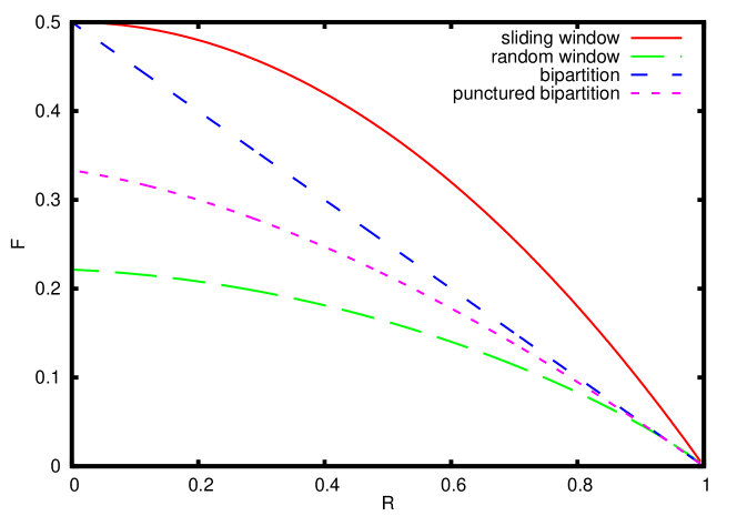
Figure 1: Comparison of the binary complexity exponents for the four classical decoding techniques applied to quantum codes at the quantum GV bound, see Sec. III. Note that for high-rate codes, $R\to 1$, the curves for the sliding window and the random window techniques have logarithmically-divergent slopes, while the slopes for the two other techniques remain finite. In this limit of $R\to 1$ the punctured bipartition technique gives the best performance.

III-B Random window (RW) technique[30, 31, 32]

Proposition 2.

Code distance $\delta n$ of a random quantum stabilizer code $[[n,Rn]]$ can be found with complexity exponent

$$F_{Bq}=H_{2}(\delta)-\textstyle\left(\frac{1-R}{2}\right)H_{2}\left(\frac{2\delta}{1-R}\right)$$ (5)

Proof.

Given a random $q$-ary linear $[n,k]$ code, we randomly choose $s=k+\tau$ positions, where $\tau=o(k)$ is some small positive number, e.g., $\tau\sim\log_{2}k$. We wish to find an $s$-set of weight $t=1$ in some unknown codeword of weight $w$. Let $M(n,s,w)$ denote the number of random trials needed to find such a set with a high probability $1-e^{-n}$. Also, let $T(n,s,w)$ be the minimum number of $(n-s)$-sets needed to necessarily cover any (unknown) $w$-set. It is easy to check[33] that

$$\textstyle{\binom{n}{w}}/{\binom{n-s}{w}}\leq T(n,s,w)\leq\textstyle{\binom{n}{w}}/{\binom{n-s}{w}}(1+\ln{\binom{n-s}{w}})$$ (6)

and that $M(n,s,w)\leq T(n,s,w)n\ln n$. Below $w=1,2,\ldots$.

RW-algorithm performs $nT(n,s,w)$ trials of choosing $s$ random positions. Each trial gives a random $k\times s$ submatrix $G_{s}$ of a (random) generator matrix $G$. It is easy to verify that $G_{s}$ has full rank $k$ with a high probability $1-q^{-\tau}$ (also, most matrices $G$ have all possible submatrices $G_{k}$ of rank $k-n^{1/2}$ or more$)$. Thus, a typical $s$-set has a subset of $k$ information bits. If the current $s$-set includes such a subset, we consider $s$ vectors $(0\ldots 010\ldots 0)$ of weight $t=1$ and re-encode them into the codewords of length $n$. Otherwise, we discard the $s$-set and proceed further. Algorithm stops once we obtain a codeword of weight $w$. The overall complexity has the order of $n^{4}T(n,s,w)$ with the binary complexity exponent

$$F_{B}=H_{2}(\delta)-(1-R)H_{2}(\delta/(1-R)).$$

For stabilizer codes, we obtain (5) using their effective rate $R^{\prime}=(1+R)/2$. ∎

Quantum codes with small distances $w\leq(n-k)^{1/2}$ and $s\sim nR^{\prime}$ meet an exponentially tight bound

$$\log_{2}T(n,s,w)\sim\log_{2}\textstyle\left(\frac{n}{n-s}\right)^{w}\sim w-w\log_{2}(1-R)$$

Exponent (5) can be further specified if codes meet the quantum GV bound (1). The corresponding exponent $F_{Bq}^{\ast}$ reaches its maximum $F_{\mathrm{max}}\approx 0.22$ at $R=0$ [Fig. 1]. By contrast, binary linear codes give exponent $F_{B}^{\ast}=(1-R)\bigl{[}1-H_{2}\left(\delta/(1-R)\right)\bigr{]}$ that achieves its maximum $0.12$ at $R\approx 1/2$.

III-C Bipartition match (BM) technique[34]

Proposition 3.

Code distance $\delta n$ of any quantum stabilizer code $[[n,Rn]]$ can be found with complexity exponent

$$F_{Cq}=H_{4}(\delta).$$ (7)

For random stabilizer codes that meet the GV bound (1),

$$F_{Cq}^{\ast}=(1-R)/2.$$ (8)

Proof.

We use a sliding (“left”) window of length $s_{l}=\left\lfloor n/2\right\rfloor$ starting in any position $i$. For any unknown vector of weight $w$, at least one position $i$ produces a window of the average weight (down to the closest integer) $v_{l}=\left\lfloor w/2\right\rfloor$. The remaining (right) window of length $s_{r}=\left\lceil n/2\right\rceil$ will have the weight $v_{r}=\left\lceil w/2\right\rceil$. We calculate the syndromes of all vectors $e_{l}$ and $e_{r}$ of weights $v_{l}$ and $v_{r}$ on the left and right windows, respectively, and try to find two vectors $\{e_{l},e_{r}\}$ that give identical syndromes, and therefore form a codeword. Clearly, each set $\{e_{l}\}$ and $\ \{e_{r}\}$ have size of order $L=(q-1)^{w/2}{\binom{n/2}{w/2}}$. Finding two elements $e_{l}$, $e_{r}$ with equal syndromes requires complexity of order $L\log_{2}L$, by sorting the elements of the combined set. Thus, finding a code vector of weight $w=\delta n$ in any classical code requires complexity of order $q^{F_{C}n}$, where $F_{C}=H_{q}(\delta)/2$. For binary codes on the GV bound, $F_{C}^{\ast}=(1-R)/2$. The arguments of the previous propositions then give exponents (7) and (8) for stabilizer codes. ∎

Note that BM-technique works for any linear code, unlike two previous techniques provably valid for random codes. It is also the only technique that can be transferred to quantum codes without any performance loss. Note also that $F_{Cq}^{\ast}$ is always below the SW exponent $F_{Aq}^{\ast}$, and is below the RW exponent $F_{Bq}^{\ast}$ for very high rates. This is due to the fact that $F_{Bq}^{\ast}\approx 1-R$ for $R\rightarrow 1$, and is twice the value of $F_{Cq}^{\ast}$.

III-D Punctured bipartition technique [35]

Proposition 4.

Code distance $\delta n$ of a random quantum stabilizer code $[[n,Rn]]$ can be found with complexity exponent

$$F_{Dq}=\textstyle{\frac{2(1+R)}{3+R}}H_{4}(\delta)$$ (9)

For random stabilizer codes that meet the GV bound (1),

$$F_{Dq}^{\ast}=(1-R^{2})/(3+R)$$ (10)

Proof.

We now combine the SW and BM techniques and consider a sliding window of length $s=\left\lceil 2nR/(1+R)\right\rceil$ that exceeds $k$ by a factor of $2/(1+R)$. It is easy to verify that most random $[n,k]$ codes include at least one information $k$-set on any sliding $s$-window $I(i,s)$. Thus, any such window forms a punctured linear $[s,k]$ code with a smaller redundancy $s-k$. Also, any codeword of weight $w$ has the average weight $v=\left\lfloor ws/n\right\rfloor$ in one or more sliding windows. For simplicity, let $s$ and $v$ be even. We then use bipartition on each $s$-window and consider all vectors $e_{l}$ and $e_{r}$ of weight $v/2$ on each half of length $s/2$. The corresponding sets $\{e_{l}\}$ and $\{e_{r}\}$ have size $L_{s}=(q-1)^{v/2}\left({}_{v/2}^{s/2}\right)$. We then seek all matching pairs $\{e_{l},e_{r}\}$ that have the same syndrome $h$. Each such pair $\{e_{l},e_{r}\}$ represents some code vector of the punctured $[s,k]$ code and is re-encoded to the full length $n$. For each $w=1,2,\ldots$, we stop the procedure once we find a re-encoded vector of weight $w$. Thus, we use $[s,k]$ punctured codes and lower BM-complexity to the order $L_{s}$.

However, it can be verified that some (short) syndrome $h$ of size $s-k$ can appear in many vectors $e_{l}$ and $e_{r}$ of length $s/2$, unlike the original BM-case. It turns out [35] that our choice of parameter $s$ limits the number of such combinations $e_{l},e_{r}$ to the above order $L_{s}$. Thus, we have to encode all $L_{s}$ code vectors of weight $v$ in a random $[s,k]$ code. The end result is a smaller complexity of order $L_{s}=q^{F_{D}n}$, where

$$F_{D}=H_{q}(\delta)R/(1+R).$$

Transition from classical codes to quantum codes does not affect BM-complexity. However, our sliding algorithm again depends on the effective quantum code rate $R^{\prime}=(1+R)/2$. This changes exponent $F_{D}$ for classical codes to exponent (9) for stabilizer codes. Quantum GV bound (1) gives (10). ∎

For random codes of high rate $R\rightarrow 1$ that meet the GV bound, this technique gives the lowest known exponents $F_{Dq}^{\ast}$ (for stabilizer codes) and $F_{D}^{\ast}=R(1-R)/(1+R)$ (for binary codes). However, it cannot be provably applied to any linear code, unlike a simpler bipartition technique. Finally, the above propositions can be applied to a narrower class of the Calderbank-Shor-Steane (CSS) codes. Here a parity check matrix is a direct sum $H=G_{x}\oplus\omega G_{z}$, and the commutativity condition simplifies to $G_{x}G_{z}^{T}=0$. A CSS code with $\mathrm{rank}\mathop{G}_{x}=\mathrm{rank}\mathop{G}_{z}=(n-k)/2$ has the same effective rate $R^{\prime}=(1+R)/2$ since both codes include $k^{\prime}=n-(n-k)/2=(n+k)/2$ information bits. It is readily verified that CSS codes have binary complexity exponents $F(R,\delta)$ given by expressions similar to Eqs. (2), (5), (7), (9), where one must substitute $H_{4}(x)$ with $H_{2}(x)/2$.

IV Linked-cluster technique

Let $\Psi(s,\ell)$ be an ensemble of regular $(s,\ell)$ LDPC codes, in which every column and every row of matrix $H$ has weight $s$ and $\ell$ respectively. The following technique is designed as an alternative to the BP technique used in [36] to find code distance. First, note that with quantum codes, BP can yield decoding failures[23], while our setting requires error-free guarantee. The second, more important, reason is that we consider very specific, self-orthogonal LDPC codes that can be used in quantum setting. These self-orthogonal codes represent very atypical elements of $\Psi(s,\ell)$ and can have drastically different parameters. In particular, the existing constructions of such codes have low distance $d$, where $\log d\sim(\log n)/2$, whereas a typical $(s,\ell)$-code has a linearly growing distance. Thus, we consider the worst-case scenario in $\Psi(s,\ell)$, which can be provably applied to any code.

For an $(s,\ell)$-code, we represent all (qu)bits as nodes of a graph $\mathcal{G}$ with vertex set $V(\mathcal{G})$ and connect two nodes iff there is a parity check that includes both positions. A codeword $\mathbf{c}$ is defined by its support $\mathcal{E}\subseteq V(\mathcal{G})$ and induces the subgraph $\mathcal{G}(\mathcal{E})$ that forms one or more clusters and has no edges outside of $\mathcal{G}(\mathcal{E})$. Generally, we will make no distinction between the set $\mathcal{E}$ and the corresponding subgraph. Note that disconnected clusters affect disjoint sets of the parity checks. This implies

Lemma 1 (Lemma 1 from Ref. [14]).

A minimum-weight code word of a $q$-ary linear code forms a linked cluster on $\mathcal{G}$.

Proof.

Let a minimum-weight support $\mathcal{E}$ include disconnected parts, say $\mathcal{E}_{1}$ and $\mathcal{E}_{2}$. These parts satisfy different parity checks. Then vectors generated by $\mathcal{E}_{1}$ and $\mathcal{E}_{2}$ belong to our code and have smaller weights. Contradiction. ∎

Linked-cluster algorithm. The following breadth-first algorithm inspects all fully-linked clusters of a given weight $w=\delta n$. Let us assume that $j=0,1,\ldots,n-1$ is the starting position in the support $\mathcal{E}$ of an unknown codeword of weight $w$. Position $j$ belongs to some $s$ parity checks which form the list $\eta=\{h_{1},\ldots,h_{s}\}$. To satisfy the parity-check $h_{1}$, we arbitrarily select some (odd) number $v_{1}$ of the remaining $\ell-1$ parity-check positions of $h_{1}$. These $v_{1}$ positions are now included in the current support $\mathcal{E}$. Any time a new position is selected, we also append the list $\eta$ with the new parity checks which include this position. We then proceed with the subsequent parity-checks $h_{2},h_{3},\ldots$ as follows. Let a check $h_{i}$ overlap with some of the parity checks $h_{1},\ldots,h_{i-1}$ in $a_{i}\leq\ell-1$ positions, and let $b_{i}$ be the number of 1s selected in these $a_{i}$ positions. Then $h_{i}$ can use only the remaining $\ell-a_{i}$ positions to pick up some $v_{i}\equiv b_{i}(\bmod\,2)$ positions. If $b_{i}$ is odd, the algorithm adds some $v_{i}\in\{1,3,\ldots\}$ positions from $h_{i}$, but (temporarily) skips this check if $b_{i}$ is even. This parity check $h_{i}$ can be re-processed in some later step $p$ as a parity check $h_{p}$ if the corresponding number $b_{p}$ is odd. The process is stopped once we add $v=w-1$ positions. The result is a binary codeword with support $\mathcal{E}$ if all processed odd-type checks are satisfied and all unprocessed checks have even overlap with $\mathcal{E}$. At this point, adding some $v_{i}=2,4,..$ symbols in any even-type check can only increase the weight of a codeword. For a $q$-ary code, we perform summation over $v_{i}=1,2,\ldots$, and need to check the rank of a matrix formed by the corresponding $w$ columns of the check matrix. For a quantum stabilizer code, we also need to verify that any obtained codeword is linearly independent from rows of $H$.

At step $i$, there are $\binom{\ell-a_{i}}{v_{i}}$ ways to select $v_{i}$ positions. Thus, the total number of choices $N_{v}$ to select $v$ positions is

$$N_{v}\leq\sum_{m\geq 1}\,\,\sum_{v_{i}\in\{1,3,\ldots\}}\delta_{v,v_{1}+\ldots+v_{m}}\prod_{i=1}^{m}\textstyle\binom{\ell-a_{i}}{v_{i}}$$

which in turn is bounded by

$$S_{v}(\ell)\equiv\sum_{m\geq 1}\,\,\sum_{v_{i}\in\{1,3,\ldots\}}\delta_{v,v_{1}+\ldots+v_{m}}\prod_{i=1}^{m}\textstyle\binom{\ell-1}{v_{i}}$$

Here $\delta_{a,b}$ is the Kronecker symbol, and $m$ is the number of terms in the decomposition $v=v_{1}+\ldots+v_{m}$.

To estimate $S_{v}(\ell)$, introduce the generating function $g_{\ell}(z)=\sum_{v}S_{v}(\ell)z^{v}$. Easy summation gives for $q=2$:

$$g_{\ell}(z)=\textstyle\left(1-f_{\ell}(z)\right)^{-1},\quad f_{\ell}(z)\equiv\frac{(1+z)^{\ell-1}-(1-z)^{\ell-1}}{2}$$ (11)

Finally, we use the contour integration of $g_{\ell}(z)$ to find the coefficients $S_{v}(\ell)$. Let $\gamma=\sinh^{-1}(1)\approx 1.135$ in the case of a binary code, and $\gamma=1/\ln 2\approx 1.443$ in the case of a $q$-ary code. We have:

Proposition 5.

A codeword of weight $\delta n$ in a $(s,\ell)$-code can be found with complexity exponent $F_{\mathrm{LC}}=\delta\log_{2}(\gamma_{\ell}(\ell-1))$, where $\gamma_{\ell}\in(1,\gamma)$ grows monotonically with $\ell$.

More precise estimates of $S_{v}(\ell)$ also give specific numbers $\gamma_{\ell}$, which can be important for small values of $\ell$. Finally note that while the cluster technique has high complexity for large $\ell$ and $\delta$, its exponent $F_{\mathrm{LC}}$ is linear in the relative distance $\delta$. In comparison, deterministic techniques of Sec. III give the higher exponents $F\propto\delta\log(1/\delta)$ in this limit. All known quantum LDPC codes with limited-weight stabilizer generators have $\delta\propto n^{-1/2}$, and the linked-cluster technique gives the lowest complexity for these codes. Note that the RW technique also gives a linear in $\delta$ exponent $F_{Bq}$ that is bounded by $\delta-\delta\log_{2}(1-R)$. Our cluster technique still lowers this exponent $F_{Bq}$ for high code rates $R\geq 1-2[\gamma\,(\ell-1)]^{-1}$.

V Conclusion

In this paper, we considered different techniques of finding code distances of stabilizer quantum codes. For sparse quantum LDPC codes, we proposed a new cluster-based technique. This technique reduces complexity exponents of the existing non-probabilistic algorithms for codes with sufficiently small relative distances. In particular, this is the case for all known families of quantum LDPC codes that have distances of order $n^{1/2}$ or less. Cluster-based technique also beats the probabilistic random-window technique for high-rate codes.

Acknowledgment. This work was supported in part by the U.S. Army Research Office under Grant No. W911NF-11-1-0027, and by the NSF under Grant No. 1018935.

References

- [1] P. W. Shor, “Scheme for reducing decoherence in quantum computer memory,” Phys. Rev. A, vol. 52, p. R2493, 1995. [Online]. Available: http://link.aps.org/abstract/PRA/v52/pR2493
- [2] E. Knill and R. Laflamme, “Theory of quantum error-correcting codes,” Phys. Rev. A, vol. 55, pp. 900–911, 1997. [Online]. Available: http://dx.doi.org/10.1103/PhysRevA.55.900
- [3] C. Bennett, D. DiVincenzo, J. Smolin, and W. Wootters, “Mixed state entanglement and quantum error correction,” Phys. Rev. A, vol. 54, p. 3824, 1996. [Online]. Available: http://dx.doi.org/10.1103/PhysRevA.54.3824
- [4] A. Y. Kitaev, “Fault-tolerant quantum computation by anyons,” Ann. Phys., vol. 303, p. 2, 2003. [Online]. Available: http://arxiv.org/abs/quant-ph/9707021
- [5] E. Dennis, A. Kitaev, A. Landahl, and J. Preskill, “Topological quantum memory,” J. Math. Phys., vol. 43, p. 4452, 2002. [Online]. Available: http://dx.doi.org/10.1063/1.1499754
- [6] H. Bombin and M. A. Martin-Delgado, “Topological quantum distillation,” Phys. Rev. Lett., vol. 97, p. 180501, Oct 2006. [Online]. Available: http://link.aps.org/doi/10.1103/PhysRevLett.97.180501
- [7] ——, “Optimal resources for topological two-dimensional stabilizer codes: Comparative study,” Phys. Rev. A, vol. 76, no. 1, p. 012305, Jul 2007.
- [8] ——, “Homological error correction: Classical and quantum codes,” Journal of Mathematical Physics, vol. 48, no. 5, p. 052105, 2007. [Online]. Available: http://scitation.aip.org/content/aip/journal/jmp/48/5/10.1063/1.2731356
- [9] R. Raussendorf and J. Harrington, “Fault-tolerant quantum computation with high threshold in two dimensions,” Phys. Rev. Lett., vol. 98, p. 190504, 2007. [Online]. Available: http://link.aps.org/abstract/PRL/v98/e190504
- [10] H. G. Katzgraber, H. Bombin, and M. A. Martin-Delgado, “Error threshold for color codes and random three-body ising models,” Phys. Rev. Lett., vol. 103, p. 090501, Aug 2009. [Online]. Available: http://link.aps.org/doi/10.1103/PhysRevLett.103.090501
- [11] S. Bravyi, D. Poulin, and B. Terhal, “Tradeoffs for reliable quantum information storage in 2D systems,” Phys. Rev. Lett., vol. 104, p. 050503, Feb 2010. [Online]. Available: http://link.aps.org/doi/10.1103/PhysRevLett.104.050503
- [12] M. S. Postol, “A proposed quantum low density parity check code,” 2001, unpublished. [Online]. Available: http://arxiv.org/abs/quant-ph/0108131
- [13] D. J. C. MacKay, G. Mitchison, and P. L. McFadden, “Sparse-graph codes for quantum error correction,” IEEE Trans. Info. Th., vol. 59, pp. 2315–30, 2004. [Online]. Available: http://dx.doi.org/10.1109/TIT.2004.834737
- [14] A. A. Kovalev and L. P. Pryadko, “Fault tolerance of quantum low-density parity check codes with sublinear distance scaling,” Phys. Rev. A, vol. 87, p. 020304(R), Feb 2013. [Online]. Available: http://link.aps.org/doi/10.1103/PhysRevA.87.020304
- [15] J.-P. Tillich and G. Zemor, “Quantum LDPC codes with positive rate and minimum distance proportional to ,” in Proc. IEEE Int. Symp. Inf. Theory (ISIT), June 2009, pp. 799–803.
- [16] A. A. Kovalev and L. P. Pryadko, “Improved quantum hypergraph-product LDPC codes,” in Proc. IEEE Int. Symp. Inf. Theory (ISIT), July 2012, pp. 348–352.
- [17] ——, “Quantum Kronecker sum-product low-density parity-check codes with finite rate,” Phys. Rev. A, vol. 88, p. 012311, July 2013. [Online]. Available: http://link.aps.org/doi/10.1103/PhysRevA.88.012311
- [18] I. Andriyanova, D. Maurice, and J.-P. Tillich, “New constructions of CSS codes obtained by moving to higher alphabets,” 2012, unpublished.
- [19] S. Bravyi and M. B. Hastings, “Homological product codes,” 2013, unpublished.
- [20] A. R. Calderbank, E. M. Rains, P. M. Shor, and N. J. A. Sloane, “Quantum error correction via codes over GF(4),” IEEE Trans. Info. Theory, vol. 44, pp. 1369–1387, 1998. [Online]. Available: http://dx.doi.org/10.1109/18.681315
- [21] R. Gallager, “Low-density parity-check codes,” IRE Trans. Inf. Theory, vol. 8, no. 1, pp. 21–28, Jan 1962.
- [22] D. J. C. MacKay, Information Theory, Inference, and Learning Algorithms. New York, NY, USA: Cambridge University Press, 2003. [Online]. Available: http://www.cs.toronto.edu/~mackay/itila/p0.html
- [23] D. Poulin and Y. Chung, “On the iterative decoding of sparse quantum codes,” Quant. Info. and Comp., vol. 8, p. 987, 2008.
- [24] K. Kasai, M. Hagiwara, H. Imai, and K. Sakaniwa, “Quantum error correction beyond the bounded distance decoding limit,” IEEE Trans. Inf. Theory, vol. 58, no. 2, pp. 1223 –1230, Feb 2012.
- [25] G. S. Evseev, “Complexity of decoding for linear codes.” Probl. Peredachi Informacii, vol. 19, pp. 3–8, 1983, (In Russian). [Online]. Available: http://mi.mathnet.ru/ppi1159
- [26] I. Dumer, “Suboptimal decoding of linear codes: partition technique,” IEEE Trans. Inf. Theory, vol. 42, no. 6, pp. 1971 –1986, Nov 1996.
- [27] K.-H. Zimmermann, “Integral hecke modules, integral generalized reed-muller codes, and linear codes,” Technische Universit at Hamburg-Harburg, Tech. Rep. Tech. Rep. 3-96, 1996.
- [28] M. Grassl, “Searching for linear codes with large minimum distance,” in Discovering Mathematics with Magma, ser. Algorithms and Computation in Mathematics, W. Bosma and J. Cannon, Eds. Springer Berlin Heidelberg, 2006, vol. 19, pp. 287–313. [Online]. Available: http://dx.doi.org/10.1007/978-3-540-37634-7_13
- [29] G. White and M. Grassl, “A new minimum weight algorithm for additive codes,” in 2006 IEEE Intern. Symp. Inform. Theory, July 2006, pp. 1119–1123.
- [30] J. S. Leon, “A probabilistic algorithm for computing minimum weights of large error-correcting codes,” IEEE Trans. Info. Theory, vol. 34, no. 5, pp. 1354 –1359, Sep 1988.
- [31] E. A. Kruk, “Decoding complexity bound for linear block codes,” Probl. Peredachi Inf., vol. 25, no. 3, pp. 103–107, 1989, (In Russian). [Online]. Available: http://mi.mathnet.ru/eng/ppi665
- [32] J. T. Coffey and R. M. Goodman, “The complexity of information set decoding,” IEEE Trans. Info. Theory, vol. 36, no. 5, pp. 1031 –1037, Sep 1990.
- [33] P. Erdos and J. Spencer, Probabilistic methods in combinatorics. Budapest: Akademiai Kiado, 1974.
- [34] I. I. Dumer, “Two decoding algorithms for linear codes,” Probl. Peredachi Informacii, vol. 25, pp. 24–32, 1989, (In Russian). [Online]. Available: http://mi.mathnet.ru/ppi635
- [35] I. Dumer, “Soft-decision decoding using punctured codes,” IEEE Trans. Inf. Theory, vol. 47, no. 1, pp. 59–71, Jan 2001.
- [36] X.-Y. Hu, M. P. C. Fossorier, and E. Eleftheriou, “On the computation of the minimum distance of low-density parity-check codes,” in Communications, 2004 IEEE International Conference on, vol. 2, June 2004, pp. 767–771.