Negative Casimir Entropies in Nanoparticle Interactions

Abstract

Negative entropy has been known in Casimir systems for some time. For example, it can occur between parallel metallic plates modeled by a realistic Drude permittivity. Less well known is that negative entropy can occur purely geometrically, say between a perfectly conducting sphere and a conducting plate. The latter effect is most pronounced in the dipole approximation, which is reliable when the size of the sphere is small compared to the separation between the sphere and the plate. Therefore, here we examine cases where negative entropy can occur between two electrically and magnetically polarizable nanoparticles or atoms, which need not be isotropic, and between such a small object and a conducting plate. Negative entropy can occur even between two perfectly conducting spheres, between two electrically polarizable nanoparticles if there is sufficient anisotropy, between a perfectly conducting sphere and a Drude sphere, and between a sufficiently anisotropic electrically polarizable nanoparticle and a transverse magnetic conducting plate.

I introduction

For more than a decade there has been a controversy surrounding entropy in the Casimir effect. This is most famously centered around the issue of how to describe a real metal, in particular, the permittivity at zero frequency. The latter determines the temperature corrections to the free energy, and hence the entropy. The Drude model, and general thermodynamic and electrodynamic arguments, suggest that the transverse electric (TE) reflection coefficient at zero frequency for a good, but imperfect metal, should vanish, while an ideal metal, or one described by the plasma model (which ignores dissipation) has this zero frequency reflection coefficient equal unity. Taken at face value, the first, more realistic scenario, means that the entropy would not vanish at zero temperature, in violation of the Nernst heat theorem, and the third law of thermodynamics. However, subsequent careful calculations showed that at very low temperature the free energy vanishes quadratically in the temperature, thus forcing the entropy to vanish at zero temperature. However, there would persist a region at low temperature in which the entropy would be negative. This was not thought to be a problem, since the Casimir free energy does does not describe the entire system of the Casimir apparatus, whose total entropy must necessarily be positive. However, the physical basis for the negative entropy region remains mysterious. For discussions of these effects see Refs. bostrom04 ; oai:arXiv.org:quant-ph/0605005 ; ellingsen07 ; oai:arXiv.org:0710.4882 ; dedkov08 ; gialsr ; bordag10 , and references therein.

More recently, negative entropy has been discovered in purely geometrical settings oai:arXiv.org:0911.0913 . Thus, in considering the free energy between a perfectly conducting plate and a perfectly conducting sphere, it was found that when the distance between the plate and the sphere is sufficiently small, the room-temperature entropy turns negative, and that the effect is enhanced for smaller spheres. For a very small sphere, the free energy and entropy are well-matched by a dipole approximation cdmnlr ; lopez .

The previous discussion suggests that this phenomenon should be studied in a systematic way. In this paper we consider the retarded Casimir-Polder interactions Casimir:1947hx between a small object, such as a nanosphere or nanoparticle, possessing anisotropic electric and magnetic polarizabilities, and a conducting plate, and we analyze the contributions to the free energy and entropy for the TE and TM (transverse magnetic) polarizations of the conducting plate. The case of a small perfectly conducting sphere above a plate is recovered by setting the electric polarizability, $\alpha$, equal to $a^{3}$, where $a$ is the radius of the sphere, and the magnetic polarizability, $\beta$, equal to $-a^{3}/2$. We also examine the free energy and entropy between two such anisotropically polarizable nanoparticles. We find negative entropy not only as an interplay between TE and TM polarizations in the plate, but even between a purely electrically polarizable nanoparticle and the TM polarization of the plate, provided the nanoparticle is sufficiently anisotropic. The previous negative entropy results are verified, and we show that even between electrically polarizable nanoparticles, negative entropy occurs when the product of the temperature with the separation is sufficiently small, provided the nanoparticles are sufficiently anisotropic. The interaction between two identical isotropic small spheres modeled as perfect conductors gives a negative entropy region, but not when they are described by the Drude model (no magnetic polarizability); but the interaction between an isotropic perfectly conducting sphere and an isotropic Drude sphere gives negative entropy. For room temperature, the typical distance at which negative entropy occurs is below a few microns.

Negative entropy between an electrically polarizable atom and a conducting plate was discussed in the isotropic case several years ago bezerra , and the extension to a isotropic magnetically polarizable atom was sketched in Ref. oai:arXiv.org:0904.0234 . The effects of atomic anisotropy and of the different polarizations of the conducting plate were not considered there. The zero-temperature Casimir-Polder interaction between atoms having both isotropic electric and magnetic polarizabilities was studied by Feinberg and Sucher feinberg , while the temperature dependence for isotropic atoms interacting only through their electric polarizability was first obtained by McLachlan lachlan ; lachlan2 . Barton performed the generalization for the magnetic polarizability at finite temperature barton . Haakh et al. more recently discussed the magnetic Casimir-Polder interaction for real atoms haakh . The anisotropic case at zero temperature for the electrical Casimir-Polder interaction was first given by Craig and Power craig ; craig2 . Forces between compact objects, which could include nanoparticles in the dipolar limit, have been considered by many authors, for example in Refs. emig06 ; emig07 ; sernelius08 ; sernelius08a , but less attention has been given to the equilibrium thermodynamics of such objects interacting.

In this paper we consider anisotropic small objects, with the symmetry axis of the objects coinciding with the direction between them or the normal to the plate, with both electric and magnetic polarizability. Because we are interested in matters of principle, we work in the static approximation, so both polarizabilities are regarded as constant, whereas most real atoms have very small, and complicated, magnetic polarizabilities. We also are not concerned here with the fact that achieving large anisotropies is likely to be difficult for real atoms rep3 , because it may be much more feasible to achieve the necessary anisotropies with nanoparticles, such as conducting needles.

We will work entirely in the dipole approximation for the nanoparticles, which is sufficient for large enough distances; for short distances higher multipoles become important noguez03 ; noguez04 . We also ignore any possibility of temperature dependence of the polarizabilities.

We use natural units $\hbar=c=k_{B}=1$, and Heaviside-Lorentz units for electrical quantities, except that polarizabilites are expressed in conventional Gaussian units.

II CP free energy between a nanoparticle and a conducting plate

We start by considering an anisotropic electrically and magnetically polarizable nanoparticle a distance $Z$ above a perfectly conducting plate. We can take as our starting point the multiple scattering formula for the interaction free energy between two bodies yale

$$F_{12}=\frac{1}{2}\operatorname{Tr}\ln(\bm{1}-\bm{\Gamma}_{0}\mathbf{T}_{1}^{E}\bm{\Gamma}_{0}\mathbf{T}_{2}^{E})+\frac{1}{2}\operatorname{Tr}\ln(\bm{1}-\bm{\Gamma}_{0}\mathbf{T}_{1}^{M}\bm{\Gamma}_{0}\mathbf{T}_{2}^{M})-\frac{1}{2}\operatorname{Tr}\ln(\bm{1}+\bm{\Phi}_{0}\mathbf{T}^{E}\bm{\Phi}_{0}\mathbf{T}^{M}),$$ (1)

where the $\bm{\Gamma}_{0}$ is the free electric Green’s dyadic,

$$\bm{\Gamma}_{0}(\mathbf{r,r^{\prime}})=(\bm{\nabla\nabla}-\bm{1}\nabla^{2})G_{0}(|\mathbf{r-r^{\prime}}|),\quad G_{0}(R)=\frac{e^{-|\zeta|R}}{4\pi R},$$ (2)

in terms of the imaginary frequency $\zeta$. The auxiliary Green’s dyadic is

$$\bm{\Phi}_{0}=-\frac{1}{\zeta}\bm{\nabla\times\Gamma}_{0}.$$ (3)

$\mathbf{T}^{E,M}_{1,2}$ are the electric and magnetic scattering operators for the two interacting bodies. Unfortunately, the EM cross term [the third term in Eq. (1)] in general does not factor into separate parts referring to each body; $\mathbf{T}^{E,M}$ refer to the whole system. The trace (denoted $\operatorname{Tr}$) includes an integral (at zero temperature) or a sum (for positive temperature) over frequencies, and an integral over spatial coordinates, as well as a sum over matrix indices. When the sum over only the latter is intended, we will denote that trace by $\operatorname{tr}$.

For the case of a tiny object, it suffices to use the single-scattering approximation, and replace the scattering operator by the potential

$$\mathbf{T}^{E}_{n}=\mathbf{V}^{E}_{n}=4\pi\bm{\alpha}\delta(\mathbf{r-R}),\quad\mathbf{T}^{M}_{n}=\mathbf{V}^{M}_{n}=4\pi\bm{\beta}\delta(\mathbf{r-R}),$$ (4)

for a nanoparticle at position $\mathbf{R}$ with electric (magnetic) polarizability tensors $\bm{\alpha}$ ($\bm{\beta}$). The approximation being made here is that the nanoparticle is a small object, and it is adequate to ignore higher multipoles. That is justified if $a$, a characteristic size of the particle, is small compared with the separation, $a\ll Z$. Therefore, since at least one of our bodies is a nanoparticle, it suffices to expand the logarithms in Eq. (1) and retain only the first term. Then we are left with the following formula for the Casimir-Polder free energy between a polarizable nanoparticle and a conducting plate,

$$F_{np}=-2\pi\operatorname{Tr}\left(\bm{\alpha}\bm{\Gamma}_{0}\mathbf{T}_{p}\bm{\Gamma}_{0}+\bm{\beta}\bm{\Phi}_{0}\mathbf{T}_{p}\bm{\Phi}_{0}\right).$$ (5)

Here $\mathbf{T}_{p}$ is the purely electric scattering operator for the conducting plate, which is immediately written in terms of the Green’s operator $\bm{\Gamma}$ for a perfectly conducting plate,

$$\bm{\Gamma}_{0}\mathbf{T}_{p}\bm{\Gamma}_{0}=\bm{\Gamma-\Gamma}_{0}.$$ (6)

II.1 $\bm{\alpha}$ polarization of nanoparticle

It is well-known levine that the Green’s dyadic for a perfectly conducting plate lying in the $z=0$ plane is for $z>0$ given by the image construction

$$(\bm{\Gamma-\Gamma}_{0})(\mathbf{r,r^{\prime}})=-\bm{\Gamma}_{0}(\mathbf{r},\mathbf{r}^{\prime}-2\mathbf{\hat{z}}z^{\prime})\cdot(\bm{1}-2\mathbf{\hat{z}\hat{z}}),$$ (7)

where the free Green’s dyadic is given by Eq. (2). Explicitly, the latter can be written as tomsk

$$\bm{\Gamma}_{0}(\mathbf{r,r^{\prime}})=-[\bm{1}u(|\zeta|R)-\mathbf{\hat{R}\hat{R}}v(|\zeta|R)]\frac{e^{-|\zeta|R}}{4\pi R^{3}},\quad\mathbf{R=r-r^{\prime}},$$ (8)

in terms of the polynomials

$$u(x)=1+x+x^{2},\quad v(x)=3+3x+x^{2}.$$ (9)

Let us first consider zero temperature. Then, if we ignore the frequency dependence of $\bm{\alpha}$, we integrate over imaginary frequency, and we immediately obtain the famous Casimir-Polder result Casimir:1947hx

$$E^{E}_{np}=-\int_{-\infty}^{\infty}d\zeta\operatorname{tr}\bm{\alpha\cdot(\Gamma-\Gamma}_{0})(\mathbf{R,R})=-\frac{\operatorname{tr}\bm{\alpha}}{8\pi Z^{4}}.$$ (10)

For nonzero $T$, we replace the integral by a sum,

$$\int_{-\infty}^{\infty}\frac{d\zeta}{2\pi}\to T\sum_{m=-\infty}^{\infty},$$ (11)

and replace the frequency by the Matsubara frequency matsubara

$$\zeta\to\zeta_{m}=2\pi mT.$$ (12)

We assume the principal axis of the nanoparticle aligns with the direction normal to the plate,

$$\bm{\alpha}=\mbox{diag}(\alpha_{\perp},\alpha_{\perp},\alpha_{z}),$$ (13)

and define the anisotropy $\gamma=\alpha_{\perp}/\alpha_{z}$. $\gamma\gg 1$ means that the nanoparticle is mostly polarizable in the direction parallel (transverse) to the plate, while $\gamma\ll 1$ means the nanoparticle is mostly polarizable in the direction normal to the plate. Then the free energy is easily obtained:

$$F^{E}_{np}=-\frac{3\alpha_{z}}{8\pi Z^{4}}f(\gamma,y),\quad f(\gamma,y)=\frac{y}{6}[(1+\gamma)(1-y\partial_{y})+\gamma y^{2}\partial^{2}_{y}]\frac{1}{2}\coth\frac{y}{2}$$ (14)

(the normalization is chosen so that $f(1,0)=1$), where $y=4\pi ZT$, $Z$ being the distance between the nanoparticle and the plate. The entropy is

$$S_{np}^{E}=-\frac{\partial}{\partial T}F_{np}^{E}=\frac{3\alpha_{z}}{2Z^{3}}\frac{\partial}{\partial y}f(\gamma,y),$$ (15)

so we define the scaled entropy by

$$s(\gamma,y)=\frac{\partial}{\partial y}f(\gamma,y).$$ (16)

For large $y$ this entropy approaches a constant,

$$s(\gamma,y)\sim\frac{1}{12}(1+\gamma),\quad y\to\infty,$$ (17)

while for small $y$,

$$s(\gamma,y)\sim\frac{1}{540}(1-2\gamma)y^{3}+O(y^{5}).$$ (18)

The entropy vanishes at $T=0$, and then starts off negative for small $y$ when $\gamma>1/2$. In particular, even for an isotropic, solely electrically polarizable, nanoparticle, where $\gamma=1$, the entropy is negative for a certain region in $y$, as discovered in Ref. bezerra The behavior of the entropy with $\gamma$ is illustrated in Fig. 1. For an isotropic nanoparticle, the negative entropy region occurs for $4\pi ZT<2.97169$, or at temperature $300$ K, for distances less than 2 $\mu$m.

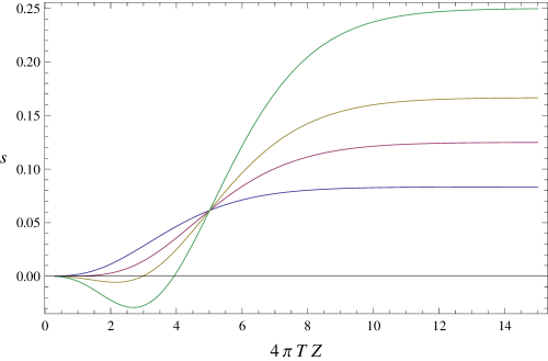
Figure 1: Scaled entropy $s$ between a purely electrically polarizable nanoparticle and a conducting plate, as a function of the product of the temperature times the distance from the plate. The different curves (bottom to top for large $ZT$) are for anisotropies $\gamma=0$ (blue), $1/2$ (red), $1$ (yellow), $2$ (green). [Color online]

Most Casimir experiments are performed at room temperature. Therefore, it might be better to present the entropy in the form

$$S_{np}^{E}=\frac{3\alpha_{z}}{2}(4\pi T)^{3}\tilde{s}(\gamma,y),\quad\tilde{s}(\gamma,y)=y^{-3}s(\gamma,y),$$ (19)

which in view of Eq. (18) makes explicit that the entropy tends to a finite value as $Z\to 0$. This version of the entropy for the isotropic case is plotted in Fig. 2.

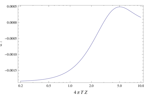
Figure 2: Rescaled entropy $\tilde{s}$ for fixed temperature as a function of the distance of an isotropic atom from the plate. The entropy tends to a finite negative value for small distances, has a positive maximum, and then decreases to zero from above for large distances.

II.2 E and H polarizations of plate

To understand this phenomenon better, let us break up the polarization states of the conducting plate. For this purpose, it is convenient to use the $2+1$-dimensional breakup of the Green’s dyadic. Following the formalism in Ref. rep3 , we find that the free Green’s dyadic has the form ($(d\mathbf{k}_{\perp})=d^{2}k_{\perp}$)

$$\bm{\Gamma}_{0}(\mathbf{r,r^{\prime}})=\int\frac{(d\mathbf{k}_{\perp})}{(2\pi)^{2}}e^{i\mathbf{k_{\perp}\cdot(r-r^{\prime})_{\perp}}}(\mathbf{\mathsf{E}+\mathsf{H}})(z,z^{\prime})\frac{1}{2\kappa}e^{-\kappa|z-z^{\prime}|},$$ (20)

which readily leads to the representation for the free energy for the nanoparticle-plate system

$$F^{E}=2\pi T\sum_{m=-\infty}^{\infty}\int\frac{(d\mathbf{k_{\perp}})}{(2\pi)^{2}}\operatorname{tr}[\bm{\alpha}\cdot(\mathbf{\mathsf{E}-\mathsf{H}})(Z,Z)]\frac{1}{2\kappa}e^{-2\kappa Z},$$ (21)

where $\kappa^{2}=k_{\perp}^{2}+\zeta_{m}^{2}$. Here the TE and TM polarization tensors are, after averaging over the directions of $\mathbf{k_{\perp}}$,

$$\mathbf{\mathsf{E}}=-\frac{\zeta^{2}}{2}\bm{1}_{\perp},\quad\mathbf{\mathsf{H}}=\frac{\kappa^{2}}{2}\bm{1}_{\perp}+(\kappa^{2}-\zeta_{m}^{2})\mathbf{\hat{z}\hat{z}}.$$ (22)

Performing the elementary integrals and sums, we get for the TE contribution to the free energy

$$F^{E}_{E}=-\frac{3\alpha_{z}}{8\pi Z^{4}}f_{E}(\gamma,y),\quad f_{E}(\gamma,y)=\gamma\frac{y^{3}}{12}\partial_{y}^{2}\left(\frac{1}{2}\coth\frac{y}{2}\right),$$ (23)

and to the entropy

$$S^{E}_{E}=-\frac{\partial}{\partial T}F^{E}_{E}=\frac{3\alpha_{z}}{2Z^{3}}s_{E}(\gamma,y),\quad s_{E}(\gamma,y)=\frac{\partial}{\partial y}f_{E}(\gamma,y).$$ (24)

For large $y$, $s_{E}$ goes to zero exponentially,

$$s_{E}(\gamma,y)\sim-\frac{\gamma}{12}y^{2}(y-3)e^{-y},\quad y\gg 1,$$ (25)

while for small $y$,

$$s_{E}(\gamma,y)\sim-\gamma\frac{y^{3}}{360}+O(y^{5}),\quad y\ll 1.$$ (26)

The transverse electric contribution to the entropy, $s_{E}$, is always negative. On the other hand, $s_{H}=s-s_{E}$ is positive for large $y$,

$$s_{H}\sim\frac{1+\gamma}{12},\quad y\gg 1,$$ (27)

but can change sign for small $y$,

$$s_{H}(\gamma,y)\sim\frac{y^{3}}{540}\left(1-\frac{1}{2}\gamma\right),\quad y\ll 1.$$ (28)

So $s_{H}$ can change sign for $\gamma>2$; the total entropy $s$, in Eq. (18), can change sign for $\gamma>1/2$. These features are illustrated in Figs. 3, 4.

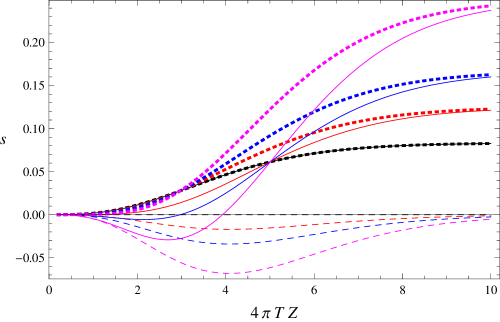
Figure 3: The entropy between an electrically polarizable nanoparticle and a conducting wall. The solid curves are the total entropy, the short-dashed curves are for the TM plate contribution, and the long-dashed curves are for TE. Referring to the ordering for large $TZ$, the inner set of curves (black) are for $\gamma=0$, the next set (red) is for $\gamma=1/2$, where the negative total entropy region starts to appear, the third set (blue) is for $\gamma=1$, and the outer set (magenta) is for $\gamma=2$. [Color online]

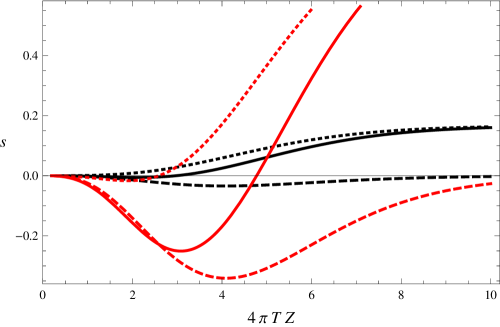
Figure 4: This illustrates that even for a solely electrically polarizable nanoparticle $S_{H}$ can turn negative for $\gamma>2$. The inner set of curves (black) are for $\gamma=1$, and the outer curves (red) are for $\gamma=10$. Again the total entropy is given by the solid curves, $s_{E}$ by the long-dashed curves, and $s_{H}$ by the short-dashed curves. [Color online]

Note that there is no difference between a perfectly conducting plate and one represented by the ideal Drude model, which differs from the former only by the exclusion of the TE $m=0$ mode. This is because this term does not contribute to $F^{E}_{E}$ or to $S^{E}_{E}$.

II.3 $\bm{\beta}$ polarization of nanoparticle

Now we turn to the magnetic polarizability of the nanoparticle, that is, the evaluation of the second term in Eq. (5). Again, from Ref. rep3 , all we need is the scattering operator for the conducting plate,

$$\mathbf{T}_{p}(\mathbf{r,r^{\prime}})=\int\frac{(d\mathbf{k}_{\perp})}{(2\pi)^{2}}e^{i\mathbf{k_{\perp}\cdot(r-r^{\prime})_{\perp}}}\frac{1}{\zeta^{2}}(\mathbf{\mathsf{E}-\mathsf{H}})(z,z^{\prime})\delta(z)e^{-\kappa|z^{\prime}|}.$$ (29)

Then the Green’s dyadic appearing there can be written in terms of the polarization operators for the plate as

$$\bm{\Phi}_{0}\cdot\mathbf{T}_{p}\cdot\bm{\Phi}_{0}(Z,Z) = \int dz^{\prime}\,dz^{\prime\prime}\int\frac{(d\mathbf{k_{\perp}})}{(2\pi)^{2}}\left(-\frac{1}{\zeta}\bm{\nabla}\times(\mathbf{\mathsf{E}+\mathsf{H}})(Z,z^{\prime})\frac{1}{2\kappa}e^{-\kappa|Z-z^{\prime}|}\right)\cdot\frac{1}{\zeta^{2}}(\mathbf{\mathsf{E}-\mathsf{H}})(z^{\prime},z^{\prime\prime})\delta(z^{\prime})$$ (30)

$$\quad\cdot\left(-\frac{1}{\zeta^{2}}\bm{\nabla}^{\prime\prime}\times\bm{\nabla}^{\prime\prime}\times-\bm{1}\right)e^{-\kappa|z^{\prime\prime}|}\cdot\left(-\frac{1}{\zeta}\bm{\nabla}^{\prime\prime}\times(\mathbf{\mathsf{E}+\mathsf{H}})(z^{\prime\prime},Z)\frac{1}{2\kappa}e^{-\kappa|z^{\prime\prime}-Z|}\right).$$

The intermediate wave operator here annihilates the following Green’s dyadic except on the plate:

$$\left(-\frac{1}{\zeta^{2}}\bm{\nabla}^{\prime\prime}\times\bm{\nabla}^{\prime\prime}\times-\bm{1}\right)e^{-\kappa|z^{\prime\prime}|}\cdot\bm{\nabla}^{\prime\prime}\times(\mathbf{\mathsf{E}+\mathsf{H}}) = \left(\frac{1}{\zeta^{2}}\nabla^{\prime\prime 2}-1\right)e^{-\kappa|z^{\prime\prime}|}\bm{\nabla}^{\prime\prime}\times(\mathbf{\mathsf{E}+\mathsf{H}})$$ (31)

$$= -\frac{2\kappa}{\zeta^{2}}\delta(z^{\prime\prime})\bm{\nabla}^{\prime\prime}\times(\mathbf{\mathsf{E}+\mathsf{H}}).$$

Now we integrate by parts and use the identities Milton:2013xia

$$\bm{\nabla}^{\prime}\times(\mathbf{\mathsf{E}-\mathsf{H}})(z^{\prime},z^{\prime\prime})\times\bm{\nabla}^{\prime\prime} = -\zeta^{2}(\mathbf{\mathsf{E}-\mathsf{H}}),$$ (32a)

$$\mathbf{\mathsf{E}}(z,z^{\prime})\cdot\mathbf{\mathsf{E}}(z^{\prime},z^{\prime\prime})=-\zeta^{2}\mathbf{\mathsf{E}}(z,z^{\prime\prime}),\quad\mathbf{\mathsf{H}}(z,z^{\prime})\cdot\mathbf{\mathsf{H}}(z^{\prime},z^{\prime\prime}) = -\zeta^{2}\mathbf{\mathsf{H}}(z,z^{\prime\prime}),\quad\mathbf{\mathsf{E}}(z,z^{\prime})\cdot\mathbf{\mathsf{H}}(z^{\prime},z^{\prime\prime})=0.$$ (32b)

In this way we find the magnetic Green’s dyadic appearing in the formula for the magnetic part of the Casimir-Polder energy (5) to be

$$\bm{\Phi}_{0}\mathbf{T}_{p}\bm{\Phi}_{0}(Z,Z)=-\int\frac{(d\mathbf{k}_{\perp})}{(2\pi)^{2}}(\mathbf{\mathsf{E}-\mathsf{H}})(Z,Z)e^{-2\kappa Z},$$ (33)

which is just negative of the corresponding expression for the electric Green’s dyadic seen in Eq. (21). Thus the expression for the magnetic polarizability contribution is obtained from the free energy for the electric polarizability by the replacement $\bm{\alpha}\to-\bm{\beta}$, and the total free energy for the nanoparticle-plate system is given by

$$F=2\pi T\sum_{m=-\infty}^{\infty}\int\frac{(d\mathbf{k_{\perp}})}{(2\pi)^{2}}\operatorname{tr}[(\bm{\alpha}-\bm{\beta})\cdot(\mathbf{\mathsf{E}-\mathsf{H}})(Z,Z)]\frac{1}{2\kappa}e^{-2\kappa Z}.$$ (34)

This simple relation between the electric and magnetic polarizability contributions was noted in Ref. oai:arXiv.org:0904.0234 . In particular, for the interesting case of a conducting sphere, the previous results apply, except multiplied by a factor of 3/2. In that case, the limiting value of the entropy is

$$S(T)\sim-\frac{4}{15}(\pi aT)^{3},\quad 4\pi ZT\ll 1.$$ (35)

III Casimir-Polder interaction between two nanoparticles

Let us now consider two nanoparticles, one located at the origin and one at $\mathbf{R}=(0,0,Z)$. Let the nanoparticles have both static electric and magnetic polarizabilities $\bm{\alpha}_{i}$, $\bm{\beta}_{i}$, $i=1,2$. We will again suppose the nanoparticles to be anisotropic, but, for simplicity, having their principal axes aligned with the direction connecting the two nanoparticles:

$$\bm{\alpha}_{i}=\mbox{diag}(\alpha^{i}_{\perp},\alpha^{i}_{\perp},\alpha_{z}^{i}),\quad\bm{\beta}_{i}=\mbox{diag}(\beta^{i}_{\perp},\beta^{i}_{\perp},\beta_{z}^{i}).$$ (36)

The methodology is very similar to that explained in the previous section.

III.1 Electric polarizability

We start with the interaction between two electrically polarizable nanoparticles. The free energy is

$$F^{EE}=-\frac{T}{2}\sum_{m=-\infty}^{\infty}\operatorname{tr}[4\pi\bm{\alpha}_{1}\cdot\bm{\Gamma}_{0}(\mathbf{R})\cdot 4\pi\bm{\alpha}_{2}\cdot\bm{\Gamma}_{0}(\mathbf{R})],$$ (37)

where the free Green’s dyadic is given in Eq. (2). In view of Eq. (8), in terms of the polynomials (9), a simple calculation yields ($y=4\pi ZT$)

$$F^{EE}=-\frac{23}{4\pi Z^{7}}\alpha_{z}^{1}\alpha_{z}^{2}f(\gamma,y),$$ (38)

normalized to the zero-temperature Casimir-Polder energy Casimir:1947hx , where

$$f(\gamma,y)=\frac{y}{23}\left[4\left(1-y\partial_{y}+\frac{1}{4}y^{2}\partial^{2}_{y}\right)+2\gamma\left(1-y\partial_{y}+\frac{3}{4}y^{2}\partial_{y}^{2}-\frac{1}{4}y^{3}\partial_{y}^{3}+\frac{1}{16}y^{4}\partial_{y}^{4}\right)\right]\frac{1}{2}\coth\frac{y}{2}.$$ (39)

Here $\gamma=\gamma_{1}\gamma_{2}$, where $\gamma_{i}=\alpha_{\perp}^{i}/\alpha_{z}^{i}$. The entropy is

$$S^{EE}=\frac{23\alpha_{z}^{1}\alpha_{z}^{2}}{Z^{6}}s^{EE}(\gamma,y),\quad s^{EE}(\gamma,y)=\frac{\partial}{\partial y}f(\gamma,y).$$ (40)

The asymptotic limits are

$$s^{EE}(\gamma,y) \sim \frac{2+\gamma}{23},\quad y\gg 1,$$ (41a)

$$s^{EE}(\gamma,y) \sim \frac{1}{2070}(1-\gamma)y^{3},\quad y\ll 1,$$ (41b)

so even in the pure electric case there is a region of negative entropy for $\gamma>1$. This is illustrated in Fig. 5.

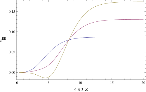
Figure 5: The entropy $s^{EE}(\gamma,y)$ for two anisotropic purely electrically polarizable nanoparticles with separation $Z$ and temperature $T$. When $\gamma=\gamma_{1}\gamma_{2}>1$ the entropy can be negative. The curves, bottom to top for large $ZT$ are for $\gamma=0$ (blue), 1 (red), 2 (yellow), respectively. (Color online)

The coupling of two magnetic polarizabilities is given by precisely the same formulas, except for the replacement $\bm{\alpha}\to\bm{\beta}$.

III.2 EM cross term

For the “interference” term between the magnetic polarization of one nanoparticle and the electric polarization of the other, we compute the free energy from the third term in Eq. (1),

$$F^{EM}=-\frac{1}{2}\operatorname{tr}[\bm{\Phi}_{0}\cdot 4\pi\bm{\alpha}_{1}\cdot\bm{\Phi}_{0}\cdot 4\pi\bm{\beta}_{2}]+(1\leftrightarrow 2).$$ (42)

This is easily worked out using the following simple form of the $\bm{\Phi}_{0}$ operator Milton:2011ed :

$$\bm{\Phi}_{0}(\mathbf{R})=-\frac{\zeta_{m}}{4\pi Z^{3}}\mathbf{R}\times(1+\zeta_{m}Z)e^{-|\zeta_{m}|Z},\quad Z=|\mathbf{R}|.$$ (43)

The result for the free energy is

$$F^{EM}=\frac{7}{4\pi Z^{7}}(\alpha_{\perp}^{1}\beta_{\perp}^{2}+\beta_{\perp}^{1}\alpha_{\perp}^{2})g(y),$$ (44)

which is normalized to the familiar zero temperature result feinberg , where

$$g(y)=\frac{y}{14}\left(y^{2}\partial_{y}^{2}-y^{3}\partial_{y}^{3}+\frac{1}{4}y^{4}\partial_{y}^{4}\right)\frac{1}{2}\coth\frac{y}{2}.$$ (45)

The entropy is

$$S^{EM}=-\frac{7}{Z^{6}}(\alpha_{\perp}^{1}\beta_{\perp}^{2}+\beta_{\perp}^{1}\alpha_{\perp}^{2})s^{EM},\quad s^{EM}(y)=\frac{\partial g(y)}{\partial y}.$$ (46)

This is always negative, vanishes exponentially fast for large $y$, and also vanishes rapidly for small $y$,

$$s^{EM}\sim-\frac{y^{5}}{7056}.$$ (47)

III.3 General results

We can present the total entropy for two nanoparticles having both electric and magnetic polarizabilities as follows,

$$S=\frac{1}{Z^{6}}\left[23\alpha^{1}_{z}\alpha^{2}_{z}s^{EE}(\gamma^{1}_{\alpha}\gamma^{2}_{\alpha},y)+23\beta^{1}_{z}\beta^{2}_{z}s^{EE}(\gamma^{1}_{\beta}\gamma^{2}_{\beta},y)-7(\alpha_{z}^{1}\beta_{z}^{2}\gamma^{1}_{\alpha}\gamma^{2}_{\beta}+\beta_{z}^{1}\alpha_{z}^{2}\gamma^{1}_{\beta}\gamma^{2}_{\alpha})s^{EM}(y)\right],$$ (48)

where $s^{EE}$ and $s^{EM}$ are given by Eqs. (40) and (46), respectively. For small $y$, the leading behavior of the entropy is

$$S = \frac{y^{3}}{90R^{6}}[\alpha^{1}_{z}\alpha^{2}_{z}(1-\gamma^{1}_{\alpha}\gamma^{2}_{\alpha})+\beta^{1}_{z}\beta^{2}_{z}(1-\gamma^{1}_{\beta}\gamma^{2}_{\beta})]$$ (49)

$$\quad\mbox{}+\frac{y^{5}}{5040R^{6}}[\alpha^{1}_{z}\alpha^{2}_{z}(4+7\gamma^{1}_{\alpha}\gamma^{2}_{\alpha})+\beta^{1}_{z}\beta^{2}_{z}(4+7\gamma^{1}_{\beta}\gamma^{2}_{\beta})+5(\alpha^{1}_{z}\beta^{2}_{z}\gamma^{1}_{\alpha}\gamma^{2}_{\beta}+\beta^{1}_{z}\alpha^{2}_{z}\gamma^{1}_{\beta}\gamma^{2}_{\alpha})+O(y^{7}).$$

In the following six figures we present graphs of the entropy for the case of identical nanoparticles, for simplicity, $\alpha_{z}^{1}=\alpha_{z}^{2}$, $\beta_{z}^{1}=\beta_{z}^{2}$, $\gamma_{\alpha}^{1}=\gamma_{\alpha}^{2}$, $\gamma_{\beta}^{1}=\gamma_{\beta}^{2}$. In Fig. 6 we show the entropy for isotropic nanoparticles with different ratios of magnetic to electric polarizabilities; negative entropy appears when the ratio is smaller than about $-1/8$. This is a nonperturbative effect, because the leading power of $y^{3}$ for small $y$ has a vanishing coefficient in this case, and the $y^{5}$ term has a positive coefficient —See Eq. (49). (The radius of convergence of the series expansions for the free energy is $|y|=2\pi$.) Thus, perfectly conducting spheres, for which the ratio of magnetic to electric polarizabilities is $-1/2$, exhibit $S<0$.

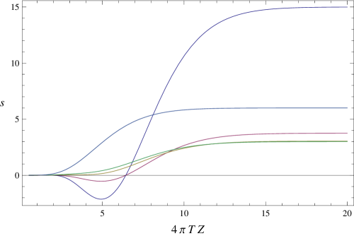
Figure 6: Entropy of two identical isotropic nanoparticles ($\gamma_{\alpha}=\gamma_{\beta}=1$) for different values of the ratio $r=\beta/\alpha$. Starting from highest to lowest curves on the left, the entropy is given for $r=1$ (purple), 0 (green),-1/8 (yellow), -1/2 (red), -2 (blue). What is plotted in this and the following figures is $s$, where the entropy is $S=[(\alpha_{z}^{1})^{2}/Z^{6}]s$. (Color online)

In Fig. 7 we examine the case of equal $z$ components of the electric and magnetic polarizabilities, but when only the electric polarizability is anisotropic. Negative entropy occurs when $\gamma_{\alpha}>1$, which we see perturbatively from Eq. (49).

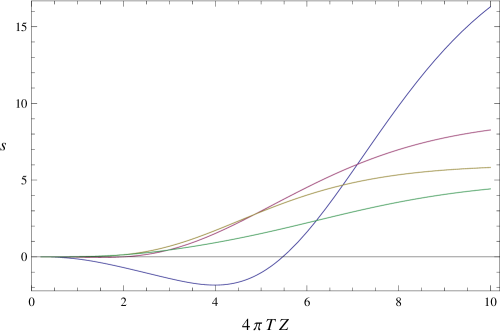
Figure 7: Here the identical nanoparticles have equal values of $\alpha_{z}=\beta_{z}$, and $\gamma_{\beta}=1$, but different values of the electric anisotropy. Reading from bottom to top on the right, we have $\gamma_{\alpha}=0$ (green), 1 (yellow), 2 (red), 4 (blue), respectively. (Color online)

In Fig. 8 we consider the nanoparticles as having equal polarizabilities and equal anisotropies. Again, as seen perturbatively, the boundary value for negative entropy is $\gamma=1$.

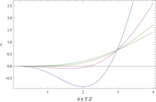
Figure 8: Here the identical nanoparticles have equal electric and magnetic polarizabilities, and equal anisotropies, which, starting from the bottom on the right, have the values $\gamma=0$ (green), 1 (yellow), 2 (red), 4 (blue), respectively. (Color online)

The case of a conducting sphere has $\beta=-\alpha/2$. We examine this situation in Fig. 9, for different magnetic anisotropies, and in Fig. 10, for different electric anisotropies. In this case the leading term in Eq. (49) vanishes at $\gamma=1$, so the appearance of negative entropy for $\gamma\leq 1$ is nonperturbative. In fact, the boundary values for the two cases are $\gamma_{\beta}=0.5436$ and $\gamma_{\alpha}=0.7427$, respectively. For the latter case, this is illustrated in Fig. 11.

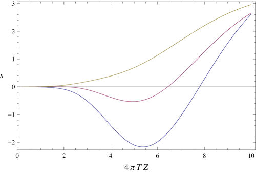
Figure 9: The case of two identical conducting spheres where $\alpha_{z}=-2\beta_{z}$, with electrical isotropy, but magnetic anisotropy $\gamma_{\beta}=0$ (yellow), 1 (red), 2 (blue), reading from top to bottom. (Color online)

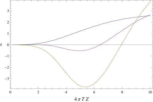
Figure 10: The case of two identical conducting nanoparticles where $\alpha_{z}=-2\beta_{z}$, with magnetic isotropy, but electric anisotropy $\gamma_{\alpha}=0$ (blue), 1 (red), 2 (yellow), reading from top to bottom in the middle. (Color online)

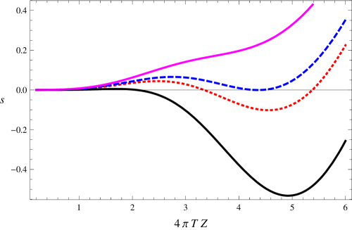
Figure 11: Two identical nanoparticles with $\beta_{z}=-\alpha_{z}/2$, appropriate for a conducting sphere, isotropic magnetically, but with electric anisotropies $\gamma_{\alpha}=0.6$ (magenta), 0.743 (dashed blue), 0.8 (short dashed red), 1 (black), shown from top to bottom.

An interesting case is the interaction of a perfectly conducting nanoparticle with a Drude nanoparticle, by which we mean that the latter has vanishing magnetic polarizability. In Fig. 12 we consider the electric anisotropies to be the same, while in Fig. 13 we show how the entropy changes as we vary the anisotropy of the magnetic polarizability of the perfectly conducting sphere. For isotropic spheres there is always a region of negative entropy.

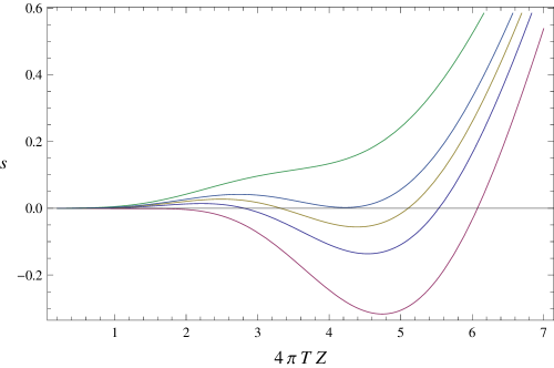
Figure 12: Interaction entropy between a small perfectly conducting nanoparticle, for which $\bm{\beta}_{1}=-\frac{1}{2}\bm{\alpha}_{1}$, and a Drude nanoparticle with the same electric polarizability and no magnetic polarizability, $\bm{\alpha}_{2}=\bm{\alpha}_{1}$, $\bm{\beta}_{2}=0$. The electric anisotropies of the two nanoparticles are assumed equal, while the perfectly conducting nanoparticle is assumed to have no magnetic anisotropy. The curves, top to bottom, are for anisotropy $\gamma_{\alpha}=0.8$ (green), $0.91$ (purple), $0.95$ (yellow), $1.0$ (blue), and $1.1$ (red), respectively. (Color online)

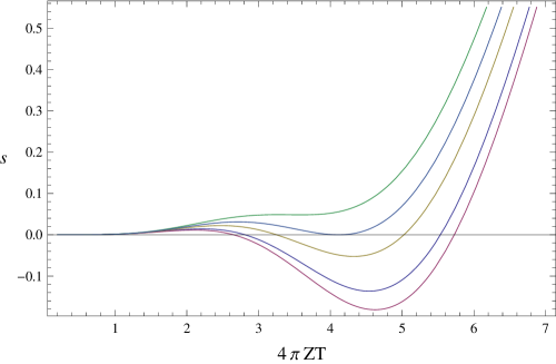
Figure 13: Interaction entropy between a small perfectly conducting nanoparticle, for which $\bm{\beta}_{1}=-\frac{1}{2}\bm{\alpha}_{1}$, and a Drude nanoparticle with the same electric polarizability and no magnetic polarizability, $\bm{\alpha}_{2}=\bm{\alpha}_{1}$, $\bm{\beta}_{2}=0$. Now it is assumed that the nanoparticles are electrically isotropic. The dependence on the magnetic anisotropy of the first nanoparticle is shown. Reading from top to bottom the magnetic anisotropies are $\gamma_{\beta 1}=0.5$ (green), 0.66 (purple), 0.8 (yellow), 1 (blue), 1.1 (red). (Color online)

IV Conclusions

In this paper we have studied purely geometrical aspects of the entropy that arise from the Casimir-Polder interaction, either between a polarizable nanoparticle and a conducting plate, or between two polarizable nanoparticles. In all cases, the entropy vanishes at $T=0$, so the issues mentioned in the Introduction concerning the violation of the Nernst heat theorem do not appear in the Casimir-Polder regime. We consider the simplified long distance regime where we may regard both the electric and magnetic polarizabilities of the nanoparticles as constant in frequency. Thus, throughout we are assuming that the separations $Z$ are large compared to the size of the nanoparticles, $a$. This same restriction justifies the use of the dipole approximation for the nanoparticles. It has been known for some time that negative entropy can occur between a purely electrically polarizable isotropic nanoparticle and a perfectly conducting plate. Here we consider both electric and magnetic polarization for both the nanoparticle and the plate. Negative entropy frequently arises, but requires interplay between electric and magnetic polarizations, or anisotropy, in that the polarizability of the nanoparticles must be different in different directions. Interestingly, although in some cases the negative entropy is already contained in the leading low-temperature expansion of the entropy, in other cases negative entropy is a nonperturbative effect, not contained in the leading behavior of the coefficients of the low temperature expansion. What we observe here extends what has been found in calculations of the entropy between a finite sphere and a plate. We summarize our findings in Table 1, which, we again emphasize, refer to the dipole approximation, appropriate in the long-distance regime, $Z\gg a$. Surprisingly, perhaps, negative entropy is a nearly ubiquitous phenomenon: Negative entropy typically occurs when a polarizable nanoparticle is close to another such particle or to a conducting plate. This is not a thermodynamic problem because we are considering only the interaction entropy, not the total entropy of the system. Nevertheless, it is an intriguing effect, deserving deeper understanding.

For confrontation with future experiments, the static approximation for the polarizabilites would have to be removed, a simple task in our general formalism. We are not aware if any present experiments concerning Casimir energies between nanoparticles and surfaces, but we hope this investigation will spur efforts in that direction.

Nanoparticle/nanoparticle
or nanoparticle/plate	Negative entropy?
E/E	$S<0$ occurs for $\gamma_{\alpha}>1$
E/M	$S<0$ always
PC/PC	$S<0$ for $\gamma_{\alpha}>0.74$ or $\gamma_{\beta}>0.54$
PC/D	$S<0$ for $\gamma_{\alpha}>0.91$ or $\gamma_{\beta}>0.66$
E/TE plate	$S<0$ always
E/TM plate	$S<0$ for $\gamma_{\alpha}>2$
E/PC or D plate	$S<0$ for $\gamma_{\alpha}>1/2$

Table 1: The table shows when a negative entropy region can occur, in different situations. Here E refers to an electrically polarizable particle, M a magnetically polarizable particle, PC means a perfectly conducting particle or plate, D means an object described by the Drude model. TE and TM refer to the transverse electric and transverse magnetic contributions to a perfectly conducting plate. The electric (magnetic) anisotropy is defined by $\gamma_{\alpha}=\alpha_{\perp}/\alpha_{z}$ ($\gamma_{\beta}=\beta_{\perp}/\beta_{z}$). Analogous results can be obtained for other cases by electromagnetic duality.

- (1) M. Boström and Bo E. Sernelius, Physica A 339, 53 (2004).
- (2) I. H. Brevik, S. A. Ellingsen and K. A. Milton, New J. Phys. 8, 236 (2006) [quant-ph/0605005].
- (3) S. Å. Ellingsen, Phys. Rev. E 78, 021120 (2008) [arXiv:0710.1015].
- (4) I. H. Brevik, S. A. Ellingsen, J. S. Høye and K. A. Milton, J. Phys. A 41, 164017 (2008) [arXiv:0710.4882].
- (5) G. V. Dedkov and A. A. Kyasov, Tech. Phys. Lett. 34, 921 (2008).
- (6) G.-L. Ingold, A. Lambrecht, and S. Reynaud, Phys. Rev. E 80, 041113 (2009) [arXiv:0905.3608].
- (7) M. Bordag and I. G. Pirozhenko, Phys. Rev. D 82, 125016 (2010) [arXiv:1010.1217].
- (8) A. Canaguier-Durand, P. A. M. Neto, A. Lambrecht and S. Reynaud, Phys. Rev. Lett. 104, 040403 (2010) [arXiv:0911.0913].
- (9) A. Canaguier-Durand, P. A. Maia Neto, A. Lambrecht, and S. Reynaud, Phys. Rev. A 82, 012511 (2010) [arXiv:1005.4294].
- (10) P. Rodriguez-Lopez, Phys. Rev. B 84, 075431 (2011) [arXiv:1104.5447].
- (11) H. B. G. Casimir and D. Polder, Phys. Rev. 73, 360 (1948).
- (12) V. B. Bezerra, G. L. Klimchitskaya, V. M. Mostepanenko and C. Romero, Phys. Rev. A 78, 042901 (2008) [arXiv:0809.5229].
- (13) G. Bimonte, G. L. Klimchitskaya and V. M. Mostepanenko, Phys. Rev. A 79, 042906 (2009) [arXiv:0904.0234].
- (14) G. Feinberg and J. Sucher, J. Chem. Phys. 48, 3333 (1968).
- (15) A. B. McLachlan, Proc. R. Soc. London, Ser. A 271, 387 (1963).
- (16) A. B. McLachlan, Proc. R. Soc. London, Ser. A 274, 80 (1963).
- (17) G. Barton, Phys. Rev. A 64, 032102 (2001).
- (18) H. Haakh, F. Intravaia, C. Henkel, S. Spagnolo, R. Passante, B. Power, and F. Sols, Phys. Rev. A 80, 062905 (2009).
- (19) D. P. Craig and E. A. Power, Chem. Phys. Lett. 3, 195 (1969).
- (20) D. P. Craig and E. A. Power, Int. J. Quantum Chem. 3, 903 (1969).
- (21) T. Emig, R. L. Jaffe, M. Kardar, and A. Scardicchio, Phys. Rev. Lett. 96, 080403 (2006) [cond-mat/0601055].
- (22) T. Emig, R. L. Jaffe, M. Kardar, and A. Scardicchio, Phys. Rev. Lett. 99, 170403 (2007) [arXiv:0707.1862].
- (23) C. E. Román-Valázquez and Bo E. Sernelius, J. Phys. A 41, 164008 (2008); arXiv:0806.2067.
- (24) C. E. Román-Valázquez and Bo E. Sernelius, Phys. Rev. A 78, 032111 (2008) [arXiv:0807.1626].
- (25) K. A. Milton, E. K. Abalo, P. Parashar, N. Pourtolami, I. Brevik, S. Å. Ellingsen, S. Y. Buhmann, and S. Scheel, “Casimir-Polder repulsion: Three-body effects,” paper in preparation.
- (26) C. Noguez, C. E. Román-Velázquez, R. Esquivel-Sirvent, and C. Villarreal, Europhys. Lett. 67, 191 (2004) [quant-ph/0310068].
- (27) C. Noguez and C. E. Román-Velázguez, Phys. Rev. B 70, 195412 (2004) [quant-ph/0312009].
- (28) K. A. Milton, P. Parashar, J. Wagner, and I. Cavero-Peláez, J. Vac. Sci. Technol. B 28, C4A8–C4A16 (2010).
- (29) H. Levine and J. Schwinger, Comm. Pure Appl. Math. III 4, 355 (1950), reprinted in K. A. Milton and J. Schwinger, Electromagnetic Radiation: Variational Methods, Waveguides, and Accelerators (Springer, Berlin, 2006), p. 543.
- (30) K. A. Milton, P. Parashar and J. Wagner, in The Casimir effect and cosmology, ed. S. D. Odintsov, E. Elizalde, and O. B. Gorbunova, in honor of Iver Brevik (Tomsk State Pedagogical University) pp. 107-116 (2009) [arXiv:0811.0128].
- (31) T. Matsubara, Prog. Theor. Phys. 14, 351 (1955).
- (32) K. A. Milton, P. Parashar, E. K. Abalo, F. Kheirandish and K. Kirsten, Phys. Rev. D 88, 045030 (2013) [arXiv:1307.2535].
- (33) K. A. Milton, P. Parashar, N. Pourtolami and I. Brevik, Phys. Rev. D 85, 025008 (2012) [arXiv:1111.4224].
- (34) K. A. Milton, J. Wagner, P. Parashar and I. Brevik, Phys. Rev. D 81, 065007 (2010) [arXiv:1001.4163].