unWISE: unblurred coadds of the WISE imaging

Abstract

The Wide-Field Infrared Survey Explorer (WISE; Wright et al. 2010) satellite observed the full sky in four mid-infrared bands in the $2.8$ to $28$ $\mu m$ range. The primary mission was completed in 2010. The WISE team have done a superb job of producing a series of high-quality, well-documented, complete Data Releases in a timely manner. However, the “Atlas Image” coadds that are part of the recent AllWISE and previous data releases were intentionally blurred. Convolving the images by the point-spread function while coadding results in “matched-filtered” images that are close to optimal for detecting isolated point sources. But these matched-filtered images are sub-optimal or inappropriate for other purposes. For example, we are photometering the WISE images at the locations of sources detected in the Sloan Digital Sky Survey (York et al., 2000) through forward modeling, and this blurring decreases the available signal-to-noise by effectively broadening the point-spread function. This paper presents a new set of coadds of the WISE images that have not been blurred. These images retain the intrinsic resolution of the data and are appropriate for photometry preserving the available signal-to-noise. Users should be cautioned, however, that the W3- and W4-band coadds contain artifacts around large, bright structures (large galaxies, dusty nebulae, etc); eliminating these artifacts is the subject of ongoing work. These new coadds, and the code used to produce them, are publicly available at http://unwise.me.

1 Introduction

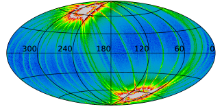
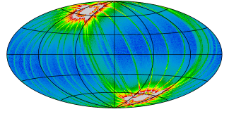
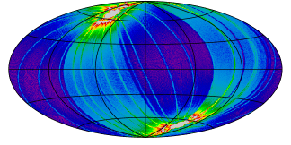
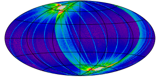
The Wide-Field Infrared Survey Explorer (WISE) mission is described in detail by Wright et al. (2010); I only briefly summarize it here. The instrument measures four infrared bands centered on 3.4 $\mu m$ (W1), 4.6 $\mu m$ (W2), 12 $\mu m$ (W3), and 22 $\mu m$ (W4), using HgCdTe arrays for the shorter W1 and W2 bands, and Si:As for W3 and W4. Survey operations began 2010 Jan 14. Coverage of the full sky was completed 2010 Jul 17. Observations continued until 2010 Aug 6, when the solid hydrogen cryogen ran out and the longest band, W4, became unusable. “Three-band” observations using the remaining W1, W2, and W3 channels continued until 2010 Sep 29, and the “NEOWISE post-cryo” program (Mainzer et al., 2011) continued observations in the shortest W1 and W2 bands until 2011 Feb 1. The WISE telescope is 40 cm and provides a field of view 47 by 47 arcmin which is imaged simultaneously via dichroics on the four detectors. Exposure time was 7.7 sec (W1 and W2) and 8.8 sec (W3 and W4). The sky was scanned from Ecliptic pole to pole, with roughly 90% overlap from scan to scan. Over 99% of the sky has 11 or more exposures in W3 and W4, and 23 or more exposures in W1 and W2. Median coverage is 33 exposures in W1 and W2, 24 in W3, and 16 in W4. Coverage increases toward the Ecliptic poles, with over $3,\!000$ exposures in each band at the poles. See Figure 2.

WISE	unWISE

Figure 1: An example image: the coadd tile containing the north Ecliptic pole (2709p666), three-band composites (W1,W2,W3). These subimages are roughly $7\times 7$ arcminutes. Left: AllWISE Release Atlas Image. Right: The unWISE coadd. The insets show a zoom-in on a region containing crowded sources. In the WISE Atlas Image they are blended together, while in the unWISE coadd they are clearly distinct. These composite images are made as per Lupton (2004).

W1	W2
W3	W4

Figure 2: WISE coverage: number of exposures in W1, W2, W3, and W4 bands including all three mission phases. The projection is a Hammer–Aitoff all-sky projection in RA,Dec with RA=180, Dec=0 in the center. The extremely high-coverage areas are the Ecliptic poles.

The pixel scale is roughly 2.75 arcseconds per pixel, and the delivered images are 1016 by 1016 pixels. The W4 images were binned 2-by-2 onboard. The 4-band primary mission collected $\sim$1.5 million four-band image sets. The 3-band phase collected $\sim 400,\!000$ three-band image sets, and the NEOWISE post-cryo phase collected $\sim 900,\!000$ two-band image sets.

The AllWISE Data Release was announced 2013 Nov 13, and includes data taken during all three mission phases. The data products in the AllWISE Release include a source catalog of nearly 750 million sources, a database of photometry in the individual frames at each source position, and “Atlas Images”: coadded matched-filtered images. The previous All-Sky Data Release also included calibration individual exposures (“level 1b” images), which I use here. The algorithms are described in considerable depth in the Explanatory Supplement documents, and the Atlas Image coadds are described by Masci and Fowler (2008). I review briefly relevant parts here.

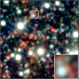
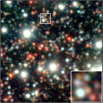
The Atlas Images in the AllWISE Release are intentionally convolved by a model of the point-spread function, producing what are sometimes called “detection maps” because they are close to optimal for detecting isolated point sources. This operation, however, blurs the images, making them less than ideal for some purposes. In this work, I produce coadds that do not include this blurring step; see Figure 1 for an example. As a result, my coadds maintain the full resolution of the original images and are appropriate for making photometric measurements. While in principle I typically advocate making photometric measurements by simultaneously forward-modeling the individual exposures, the WISE instrument is remarkably stable and has a nearly isotropic point-spread function, so creating a coadd results in little loss of information about the non-variable sky.

The WISE Atlas Images (and my coadds) start with the calibrated “level 1b” individual exposures. These have been calibrated astrometrically and photometrically, flat-fielded, and had static artifacts (bad pixels, etc) flagged. The first step is selecting the frames to be included in the coadd. The criteria used (which I also follow) are to omit W3 and W4 frames within 2000 seconds of an annealing event (the W3 and W4 Si:As arrays were periodically heated—“annealed”—to remove latent images); frames with a bad frame-level quality-assurance score from the WISE image-processing pipeline; and frames taken during some on-orbit experiments. For each frame, the photometric calibration is applied to convert the images to common units. Next, background level matching is performed by matching the median of a new image to that of the existing coadd, in the pixels where they overlap. Frames suspected of being affected by moon-glow are subjected to tests on their pixel distributions; a rapidly-varying background due to moon glow increases the pixel RMS significantly above that of an image not affected by the moon. Downstream, the coadding process uses median statistics, so is quite robust to outliers; some moon-contaminated frames can be tolerated, but moon-contaminated frames are rejected if they form too large a fraction of the frames. Next, all frames to be included in the coadd are projected and interpolated onto the coadd frame in order to detect outliers. A “pixel overlap-area weighting method,” or top-hat interpolation kernel, is used in this step. The list of interpolated pixel values for each coadd pixel is stored so that robust statistics (the median and approximate median-of-absolute differences) can be computed pixelwise. A set of heuristics is used to flag outlier pixels using the computed robust statistics. An additional set of heuristics expands masked regions so that regions containing several masked pixel become completely masked. Finally, after outlier masking, the final interpolation is performed. This uses an approximation to “pixel response function” weighting, equivalent to first smoothing the image by its point-spread function and then resampling that image. In practice, a sub-pixelized PRF representation and nearest-neighbor interpolation are used.

Top-hat	Fine top-hat	Lanczos-3	Lanczos-5

Figure 3: Comparison of “pixel overlap” (or “top-hat”; used in the AllWISE release; left) and Lanczos (used in the unWISE coadds; right) resampling, in one dimension. In this demonstration, I shift (by resampling) the signal by 0.2 pixels, and then shift the resampled signal back. In the second column (“Fine top-hat”), the resampled pixels are at twice the original pixel resolution (as done in the AllWISE Release). Top: A row of pixels; in the “pixel overlap” view, pixels are little boxes, while in my view they are samples of an underlying function. The original signal is shown by the faint green line, and the result after resampling by 0.2 pixels and then sampling back is shown in solid blue. Middle row: Resampling error: difference between resampled and original signal. Bottom: Repeating this process of resampling the signal back and forth 30 times results in marked smoothing of the signal in the case of pixel overlap resampling, but little loss of fidelity for the case of Lanczos resampling. The signal is a mixture of two Gaussians so is technically not band limited; some aliasing error is to be expected.

The primary difference between my coadds and those of the AllWISE Release is in the interpolation kernels we use. This belies a difference in philosophy as well. The WISE Explanatory Supplement documents describe pixels as though they are “little boxes”. This picture leads to confusion and heuristics with no theoretical basis in sampling or information theory. Unfortunately, this “pixels are little boxes” view has persisted for some time in astronomical image processing, perhaps most strikingly in the form of the “drizzle” process predominantly used for Hubble Space Telescope images (Fruchter and Hook, 2002). In contrast, I think of detector pixels as taking (noisy) delta-function samples of an underlying smooth, continuous function: the pixel-convolved point-spread function convolved with the scene. Once the pixels have been read out, it is not necessary or helpful to think of them as “little boxes”; they are simply samples of an underlying two-dimensional function. As I show below, the WISE pixels well-sample the point-spread function and thus this underlying function, so the Nyquist–Shannon sampling theorem applies; a discrete set of samples contains sufficient information to reconstruct the original signal.

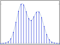
Briefly, the Nyquist–Shannon sampling theorem, in one dimension, states that if a continuous function contains no frequency components above a band-limit frequency $B$, then a discrete set of samples spaced $1/2B$ apart completely characterise the function; the original function can be reconstructed exactly through sinc interpolation of the samples. A good review article is Jerri (1977). In the context of astronomical images, an image satisfies the sampling criterion—it is “well-sampled”—if the underlying function contains no spatial frequency components (Fourier modes) shorter than 2 pixels. In that case, a discrete set of image pixels (samples) are sufficient to completely characterise the underlying function. As mentioned above, the underlying function is the astronomical scene convolved by the pixel-convolved point-spread function; since the scene can contain (nearly) point sources, the well-sampled condition depends on the pixel size relative to the pixel-convolved point-spread function. Given a well-sampled image, we can resample it to a different pixel grid, without loss of information—as long as the target pixel grid also well-samples the image—through sinc interpolation. The sinc function is the Fourier transform of the ideal low-pass filter, leaving all frequencies below the band limit untouched and removing all frequencies above it. The sinc interpolation kernel has infinite extent, so in practice we taper the sinc kernel to give it finite extent. In this work, I use the popular Lanczos kernel as a tapered approximation to the sinc kernel.

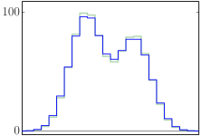
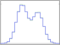
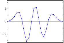
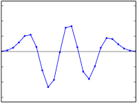
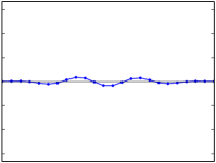
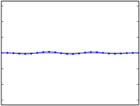
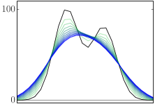
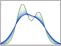
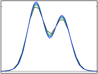
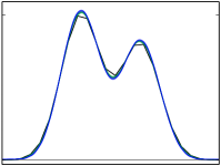
Figure 3 shows the loss of information resulting from using the top-hat kernel compared to the Lanczos kernel.

W1	W2	W3	W4

Figure 4: Top row: WISE individual-exposure PSF models from Meisner et al. (2014), at the center of the field of view, shown on a log scale with dynamic range $10^{7}$, and size $250\times 250$ pixels. Middle row: Slices through the PSF model in the $x$ and $y$ directions, plus the critically-sampled Airy profile, $(4\mathrm{J}_{1}(\pi x/2)/(\pi x))^{2}$; the PSF models are only a little wider. Bottom row: Power spectra of 1-d slices of the PSF models in the $x$ and $y$ directions, along with critically-sampled Airy profile and a Gaussian with the same full-width at half max ($\sigma\sim 0.88$). The PSF models have a small amount of power outside the band limit, roughly comparable to the Gaussian. These PSF models are constructed from WISE data so include some noise which also contributes to the power spectrum. The leftmost (W1) panel also shows the power spectrum of the Lanczos-3 interpolation kernel used in this work: it is mostly flat, but slightly attenuates high-frequency components. When I measure isolated point sources in the individual exposures or the unWISE coadds, I find similar profiles and power spectra.

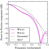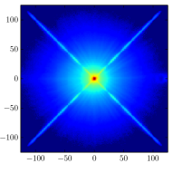
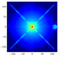
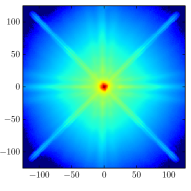
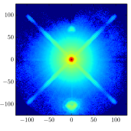
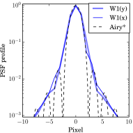
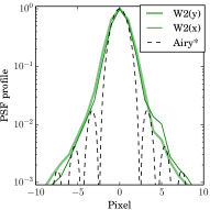
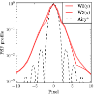
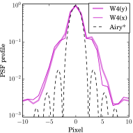
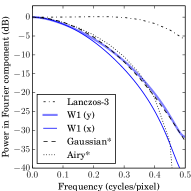
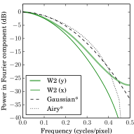
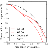
Figure 4 shows the WISE point-spread function models from Meisner et al. (2014) and their Fourier transforms. These models are constructed by combining a large number of bright stars (to get the wings) and moderately bright stars (to get the core, which is saturated in bright stars). The PSF profiles roughly follow the envelope of an Airy profile scaled to be critically sampled, suggesting that the WISE images are approximately critically sampled. The full-widths at half-max quoted in the WISE Explanatory Supplement are 6.1 and 5.6 arcseconds for the major and minor axes in W1, 6.8 and 6.1 for W2, 7.4 and 6.1 for W3, and 12.0 and 11.7 for W4; for comparison, the rule-of-thumb of $\sim 2.1$ pixels across the FWHM (which is derived from the width of the critically-sampled Airy profile) would be 5.7 arcseconds. The Fourier transform of the PSF models shows a small amount of power at the band limit, comparable to that of a Gaussian whose full-width at half-maximum equals that of the critically-sampled Airy. In practice, this indicates that we can treat the WISE images as well-sampled; if there is indeed power outside the band limit, we will incur a small aliasing error when we resample the images.

In the case of the WISE Atlas Images, in addition to resampling to the coadd pixel grid, there is also an extra convolution by the point-spread function. In order to avoid the issues with top-hat resampling shown in Figure 3, the Atlas Image pixels were chosen to have twice the resolution of the input images. In contrast, I do not perform any additional convolutions on the input images, and I produce coadds at the original nominal pixel scale. The resulting point-spread function widths are roughly $8.5$ arcseconds FWHM for the AllWISE Release Atlas Images in W1, W2, and W3 bands, versus roughly $6$ arcseconds for my coadds; the W4 PSF is roughly twice as wide.

2 Method

The overall procedure follows that of the AllWISE Release, though in general each step is simpler. I have used the high-quality data products provided by the WISE pipeline as far as possible. I use the same RA,Dec centers and axis-aligned orientations as the Atlas Image tiles. My coadds are $2048\times 2048$ pixels at the nominal native pixel scale, $2.75$ arcseconds per pixel, rather than the $4095\times 4095$ images at $1.375$ arcseconds per pixel chosen in the AllWISE Release. Since the WISE images are well sampled, there is nothing to be gained in my formulation by producing coadds at double the resolution of the inputs. For the sake of consistency, my W4 coadds are on the same $2.75$ arcsecond per pixel grid as the other bands, even though the input images have only half the resolution.

I produce a coadd in two phases. In the first, I accumulate an initial mean and variance estimate for the coadd pixels and use this to mask outlier pixels in the input frames. I mask and patch these pixels, then produce the final coadd.

I select input frames from all three mission phases that touch the RA,Dec box of the target coadd tile. I remove any frames with WISE pipeline-assigned frame-level quality score of zero. For W3 and W4, I remove frames within 2000 seconds of an anneal. For W4, I remove scans in the range 03752a to 03761b inclusive (as do the WISE team), in which the W4 bias level was changed for testing purposes.

I drop frames that appear to be contaminated by scattered moonlight, following the procedure used by the WISE team. After all other cuts have been made, I examine frames that are not within the moon mask (ie, unlikely to be strongly affected by moon-glow). I use the robust estimate of the pixel standard deviation measured in the WISE pipeline (the median minus 16^th percentile), computing the median and median absolute difference of this quantity in the uncontaminated frames. This roughly characterizes the “typical” background variations in the coadd tile. I reject any frame within the moon mask whose pixel standard deviation is greater than the median plus 5 median absolute differences times a Gaussian correction factor of $1.4826$.

Resampled image ($I_{i}$)	Mask ($M_{i}$)	Unmasked pixels ($G_{i}$)

Figure 5: Image products produced per input frame in the first-round coadds, shown for two input frames, for a small $200\times 200$-pixel cutout in one W1 coadd tile. Left: the Lanczos-resampled image. Middle: the binary mask indicating which coadd pixels are touched by this input frame. Right: the per-pixel masks, nearest-neighbor resampled to the coadd frame.

Coadded image ($C$)	Coadded weights ($W$)	Per-pixel std. dev. ($S$)

Figure 6: Coadded image products produced in the first-round, for a small $200\times 200$-pixel cutout in one W1 coadd tile. Left: the coadded intensity image. Middle: the summed weights (inverse-variances). Right: the per-pixel standard deviation.

Coadded image ($C_{1}$)	Per-pixel std. dev. ($S_{1}$)
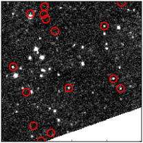
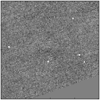
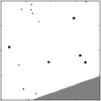
Resampled image ($I_{i}$)	Chi vs coadd ($\chi_{i}$)	Outlier pixels

Figure 7: Outlier pixel detection using per-pixel sample statistics. This is the same small W1 region as in Figures 5 and 6. Top row: First-round coadd and per-pixel standard deviation. Thanks to Poisson statistics, the per-pixel standard deviation is larger where sources are found. This avoids falsely marking too many pixels near sources as outliers. Middle and Bottom rows, left: Resampled images, with the locations of detected outlier pixels marked. Pixels near sources are occasionally falsely mark as outliers. Center: Chi: resampled image minus coadd mean, divided by per-pixel standard deviation (after removing image $i$ from the mean and standard deviation estimates). The large blemishes in the bottom row are readily identified. Right: Pixels with absolute value of chi greater than 5 are marked as outliers.

I then read each frame in turn, along with its uncertainty image and masked-pixels image. I scale each intensity image and its uncertainty image, using the WISE pipeline zeropoints, to have a zeropoint of $22.5$. This is, a source with integrated flux of unity in these images (and thus the coadds) corresponds to a Vega magnitude of $22.5$. I estimate an image-wide standard deviation, $\sigma_{i}$, based on the median of unmasked pixels in the uncertainty image. The uncertainty images (produced by the WISE pipeline) include read noise and pixelwise Poisson noise from sources, but I want a single image-wide scalar to avoid biases; the median yields roughly the read noise plus sky background noise. I use the inverse-variance as the weight $w_{i}$ for image $i$; weight $w_{i}={\sigma_{i}}^{-2}$.

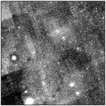
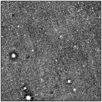
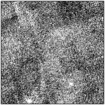
I find that many of the W3 and W4 images have spatially varying background levels that appear to be instrumental rather than astrophysical. I apply a simple approximate spatial median filter on the input frames in order to remove some of this background variation. A full median filter is too expensive so I compute the median in sub-images of side length $101$ pixels, then interpolate between the sub-image medians using a piecewise parabolic kernel. This will of course also remove astrophysical spatially varying backgrounds, which leads to severe artifacts in and around extended structures such as large galaxies and nearby star-forming regions. This is discussed below and illustrated in Figures 12 and 13.

In order to resample the images, I patch masked pixels, in a crude manner. For each masked pixel, I take the average of its four neighboring pixels, ignoring masked neighbors. I iterate this process until no pixels remain to be patched. The resulting images have reasonable values in all masked pixels. As a result, I do not need to handle masked pixels specially in the interpolation step; if I did not patch the images, then a single masked pixel would invalidate an image region the size of the support of the interpolation kernel (dozens of pixels). Patching the images allows me to perform the interpolation with a small approximation error. I propagate the masks (via nearest-neighbor resampling) to avoid including pixels that are dominated by patched values in the coadd.

Next, I estimate and subtract a (scalar) background level from each frame. I have taken a somewhat different approach than the WISE team, based on finding the mode of the pixel value distribution. Details are given in section 2.1 below. For W3 and W4, which have already had a median-filtered background subtracted, this additional background subtraction has little effect.

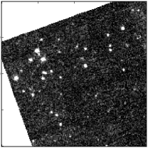
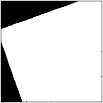
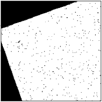
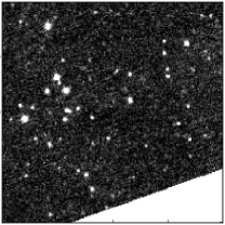
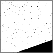
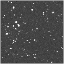
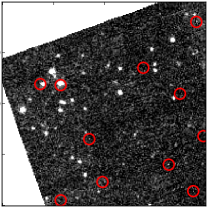
Next, I resample the input frames onto the output coadd frame. As mentioned above, the sinc interpolation kernel can be used to perform this interpolation without loss of information. The sinc has infinite extent, so I use the third-order Lanczos kernel as an approximation (see section 2.1 below). For each input frame, I compute a number of interpolated values: The image itself (Lanczos-interpolated), $I_{i}$, a binary image indicating which coadd pixels are touched by input pixels (nearest-neighbor interpolated), $M_{i}$, and a binary image indicating which input pixels were unmasked, or “good” (also nearest-neighbor interpolated), $G_{i}$; see Figure 5. From these, I accumulate three images:

$$V_{w} =\sum_{i}I_{i}^{2}M_{i}w_{i}$$ (1)

$$K_{w} =\sum_{i}I_{i}M_{i}w_{i}$$ (2)

$$W =\sum_{i}M_{i}w_{i}$$ (3)

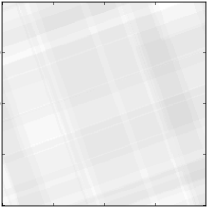
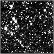
where $V_{w}$ is the weighted variance image, $K_{w}$ the weighted coadd, and $W$ the sum of (masked) weights. Recall that $I_{i}$ and $M_{i}$ are images, while $w_{i}$ is a scalar (the image-wide inverse variance described above). The first-round coadd $C_{1}$ and the per-pixel sample standard deviation $S_{1}$, are:

$$C_{1} =\frac{K_{w}}{W} S_{1} =\sqrt{\frac{V_{w}}{W}-C_{1}^{2}}\quad;$$ (4)

see Figure 6.

Using the per-pixel sample variance computed in the first-round coadd, I detect pixels that are significant outliers. In order to avoid outliers themselves biasing the estimated sample mean and variance, I have to remove each frame’s contribution from the sample mean (coadd) and sample variance,

$$C_{i} =\frac{K_{w}-I_{i}M_{i}w_{i}}{W-M_{i}w_{i}} S_{i}^{2} =\frac{V_{w}-I_{i}^{2}M_{i}w_{i}}{W-M_{i}w_{i}}-C_{i}^{2}\quad.$$ (5)

Furthermore, since the sample variance estimate given a small number of samples can be noisy, I apply a prior on the variance, $P_{i}^{2}$, to get a regularized variance estimate $\hat{S}_{i}^{2}$:

$$P_{i}^{2} =\sigma_{i}^{2}+(eC_{i})^{2}$$ (6)

$$\hat{S}_{i} =\sqrt{\frac{S_{i}^{2}(W-M_{i}w_{i})+P_{i}^{2}\,\nu w_{i}}{W-M_{i}w_{i}+\nu w_{i}}}$$ (7)

where $e$ is a multiplicative flux error (set to $3\%$; see section 3), and $\nu$ is the effective weight of the prior (set to $5$); this is similar to a Gamma prior. Using these estimates of the mean and standard deviation, I compute the per-pixel chi value,

$$\chi_{i} =\frac{I_{i}-C_{i}}{\hat{S}_{i}}\quad,$$ (8)

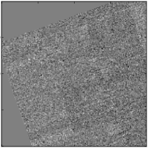
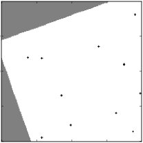
and mask any pixel $i$ with $\lvert\chi_{i}\rvert>5$ as an outlier. See Figure 7. This readily removes artifacts such as cosmic rays and satellite trails, and will also remove transient or fast-moving sources. I mask the 4-connected neighbors of masked pixels as well, resample these masks back to the original image frame via nearest-neighbor interpolation, and record them for future use. I discard any frame that has more than 1% of its pixels masked. I then patch the frame’s resampled image and accumulate it into the second-round coadds.

During the second round, I patch outlier pixels, and add the outliers to the pixel masks:

$$J_{i} =\textrm{patch}(I_{i}\,,\,\lvert\chi_{i}\rvert>5) H_{i} =G_{i}\wedge(\lvert\chi_{i}\rvert\leq 5)$$ (9)

(where $\wedge$ denotes binary AND) and then proceed to accumulate “unmasked” and “masked” values:

$$V_{u} =\sum_{i}{J}_{i}^{2}M_{i}w_{i} V_{m} =\sum_{i}{J}_{i}^{2}H_{i}w_{i}$$ (10)

$$K_{u} =\sum_{i}J_{i}M_{i}w_{i} K_{m} =\sum_{i}J_{i}H_{i}w_{i}$$ (11)

$$W_{u} =\sum_{i}M_{i}w_{i} W_{m} =\sum_{i}H_{i}w_{i}$$ (12)

$$N_{u} =\sum_{i}M_{i} N_{m} =\sum_{i}H_{i}$$ (13)

and at the end, the coadd products are:

$$C_{u} =\frac{K_{u}}{W_{u}} C_{m} =\frac{K_{m}}{W_{m}}$$ (14)

$$S_{u} =\frac{\sqrt{\frac{V_{u}}{W_{u}}-C_{u}^{2}}}{\sqrt{N_{u}-1}} S_{m} =\frac{\sqrt{\frac{V_{m}}{W_{m}}-C_{m}^{2}}}{\sqrt{N_{m}-1}}$$ (15)

where the difference between the “masked” $C_{m}$ and “unmasked” $C_{u}$ is that the masked versions ignore masked pixels in the input images (including pixels flagged as outliers), while the unmasked versions use the “patched” pixel values for masked pixels rather than ignoring them altogether. The per-pixel sample standard deviations $S_{m}$ and $S_{u}$ are scaled so that they are approximate error estimates for the coadd intensity pixels.

Finally, I re-estimate and subtract a scalar background level from the final coadds. This might seem to be unnecessary, since I subtracted the background from the input frames going into the coadd. But the coadds have considerably higher signal-to-noise; a pixel with one sigma of source flux in the individual frames will appear to be a blank pixel affected only by the background, but in the coadd it will have several sigma of source flux, and will no longer be considered part of the “blank” sky that defines the background level. In this way, the coadd’s pixel distribution preferentially shifts pixels with positive flux out of the “blank sky” peak into the “source” tail, meaning that the peak of the remaining “blank sky” pixel distribution is shifted negative.

The output products include, for each coadd tile: (a) co-added intensity images that exclude masked outliers and masked input pixels, $C_{m}$, as well as ones that replace these masked pixels by patching, $C_{u}$; (b) pixelwise inverse-variance maps $W_{m}$ and $W_{u}$; (c) per-pixel sample standard deviation maps $S_{m}$ and $S_{u}$; (d) number-of-frames coverage maps $N_{m}$ and $N_{u}$; (e) FITS tables summarizing the frames considered for inclusion in the coadd; and (f) mask images for the input-frame pixels flagged as outliers.

2.1 Implementation Details

I estimate a scalar background level in each input frame as follows. I attempt to find the mode of the image pixel distribution by histogramming image pixels in a region around the peak and fitting a parabola to the log-counts in each histogram bin; this assumes a Gaussian distribution of pixel values around the mode. I first produce a coarsely-binned pixel histogram, find the largest bin, then find the range of bins containing more than 50% as many pixels (on the low side) and 80% as many pixels (on the high side). I histogram this region more finely and fit a parabola to the log-counts. This region has many counts in each histogram bin and is not too contaminated by pixels with significant source flux. The WISE pipeline’s dynamic calibration (dynacal) stage is known to introduce an artifact in which a large fraction of pixel values are set to the median value; to alleviate this problem I add Gaussian noise with variance equal the per-pixel variance before histogramming the pixel values.

Resampling the input frames onto the output coadd frame requires a large number of astrometric World Coordinate System (WCS) transformations. Since these can be expensive, I use a spline approximation: I evaluate the WCS on a $25\times 25$-pixel grid, mapping coadd pixel coordinates to input coordinates, and use a cubic spline to interpolate this mapping. A similar approach is used in SWarp (Bertin et al., 2002).

I use third-order Lanczos interpolation to resample the input frames. This requires a large number of evaluations of the Lanczos kernel (a windowed sinc function), which can be quite expensive. I approximate this using a precomputed look-up table with 2048 bins per unit interval. This incurs negligible approximation error in practice.

3 Results

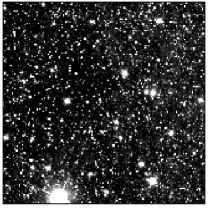
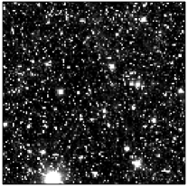
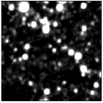
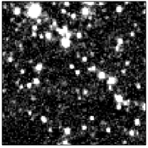
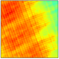
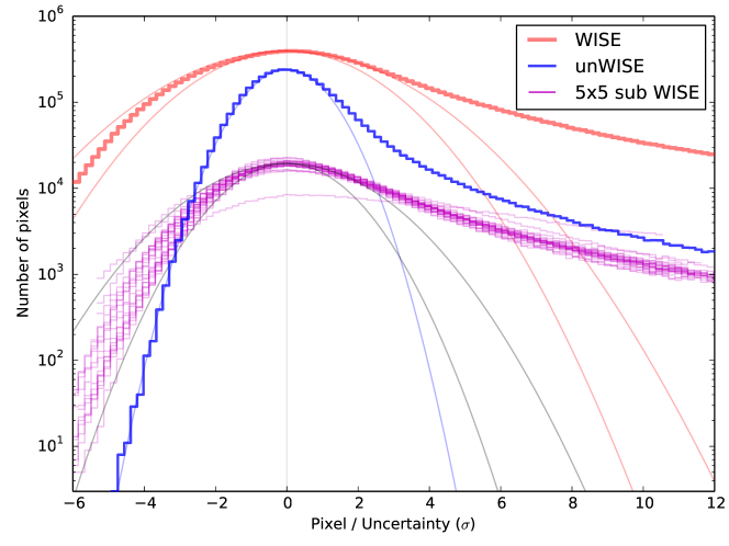
An example coadd image is shown in Figure 8.

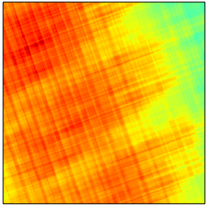
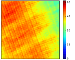
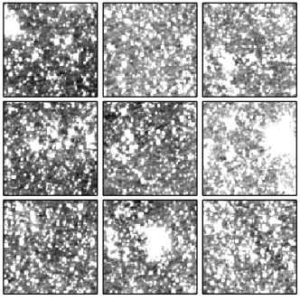
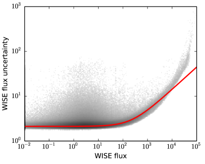
Figure 9 shows the distribution of pixel values with respect to their error estimates. I find that the AllWISE Release coadd uncertainty values appear to underestimate the variation in pixel values, at least at full-tile scales: The distribution of pixel values in full Atlas Image tiles is considerably broader than expected for a flat background. This could be due to spatial variations in the background, but since the same variations are not seen in my coadds, I expect this could be due to variations in the AllWISE Release background estimates, rather than true variations in the background levels. The method involves matching the background of an incoming frame with the existing coadd; thus “the final background level in a co-add is dictated by the first frame that was [re]projected.” An example is shown in Figure 10.

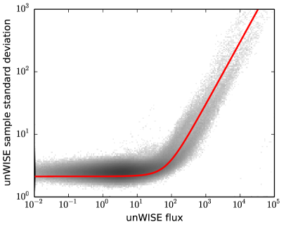
Figure 11 examines the behavior of my per-pixel sample standard deviation measurements. This can be seen as a measurement of the uncertainty of the coadd based on the data values encountered during coadding. Interestingly, there are considerable differences between this measurement of uncertainty and the “error propagation” approach used in the AllWISE Release; this could be explained by multiplicative systematics of about 3%. I suspect the AllWISE Release Atlas Images are also affected by this systematic scatter.

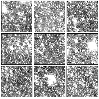
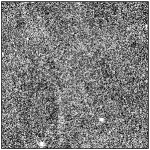
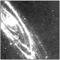
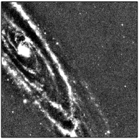
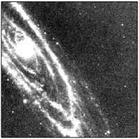
Figure 12 demonstrates the effect of applying a spatial median filter to estimate and remove a varying background from the input frames before coadding them. As expected, the median filter removes large-scale structure from the coadds, but also depresses the background levels around bright sources. A more extreme case of this is shown in Figure 13.

As outlined above, I perform two rounds of coadding, where the first round is used to reduce the impact of artifacts. In my implementation, I perform the resampling once, keeping the resampled input frames in memory until the second round. The memory required thus increases with the number of pixels touching the coadd tile. In practice, this has not proven to be problematic: the tile containing the north ecliptic pole (2709p666) has nearly $5,\!000$ W1 exposures at its peak and is touched by approximately $10^{10}$ input-frame pixels in $20,\!000$ exposures. Producing this coadd tile required peak memory of about $100$ Gbytes and took about $12$ hours on a single CPU core. The tile shown in Figure 8, 1384p454, is more typical: it is covered by $432$ exposures in W1, incorporates a total of $\sim 3\times 10^{8}$ input pixels, and took peak memory of $2.3$ GB and $630$ seconds on a single CPU core.

WISE	unWISE (unmasked)	unWISE (masked)

Figure 8: One example image: coadd tile 1384p454, band W1. Top row: Intensity images. Overall, my coadds and the AllWISE Release coadds are very similar. Second row: Zoom-in of intensity images to middle 5% of image. Here it is clear that the AllWISE Release coadds have been artificially blurred, while mine maintain full resolution. Bottom row: Number of images included in coadd.

Figure 9: Coadd pixel distributions for example tile 1384p454, band W1. Each curve shows the coadd intensity values divided by the per-pixel uncertainty values. The broad histogram labeled “WISE” shows the AllWISE Release intensity over uncertainty maps, after estimating and removing a scalar background using the method described above. In the absence of sources and varying backgrounds, this should approximate a Gaussian with unit standard deviation. Sources add the positive tails, and a varying background would broaden the distribution. The AllWISE Release pixel distribution is considerably broader than expected (the uncertainty maps do not capture the pixel variations) by more than a factor of two (the top thin guidelines are Gaussians with standard deviations 2 and 2.5). Splitting the image into $5\times 5$ subimages, the subimage distributions show a slightly narrower distribution, though still broader than expected (the guidelines show Gaussians with standard deviations $\sqrt{2}$ and 2); the $20\times 20$ subimages (not shown here) are similar. This suggests that if background variations are responsible for this effect, the relevant scale is smaller than $\sim 200$ pixels. This effect was less pronounced in the All-Sky Release Atlas Images. The curve labeled “unWISE” shows the unWISE coadd image times square root of inverse-variance maps, with no scaling or adjustments. This distribution is very close to unit Gaussian (plus source tail). The WISE curves are shifted higher because the WISE coadds have a smaller pixel scale and hence more pixels.

WISE	unWISE

Figure 10: Zoom-ins of corners of the W1 coadd tile 1384p454, to show variations in the background levels. These variations would explain the broader-than-expected distribution of pixel values relative to the uncertainty estimates seen in the WISE coadds (see Figure 9). My unWISE coadds seem to have considerably less variation.

WISE	unWISE

Figure 11: Pixelwise distributions of intensity (flux) and error estimates, for W1 tile 1384p454. Left: WISE intensity and uncertainty maps. Note the log-log scales; the fluxes are scaled to zeropoint 22.5; ie, these are “Vega nanomaggies”. At low flux levels, the error is dominated by read noise and background Poisson noise. At high flux level, the Poisson contribution from the sources becomes significant. The AllWISE Release uncertainty estimate comes from propagating the error estimates from the input frames forward through the coaddition process, and does not include any systematic uncertainties. Right: unWISE intensity and per-pixel standard deviation estimates, on the same axes. This error estimate is based on the sample variance computed during coaddition. Since it is based on the actual data values encountered, it includes systematic effects that produce scatter (but not bias). The red curves are rough by-eye “fits” of the expected behaviors. The WISE curve includes a constant noise floor plus Poisson noise whose standard deviation goes as the square root of flux. The unWISE curve includes those same components plus a component whose standard deviation goes as the flux. This would be expected if there were multiplicative systematic errors; for example, if there were scatter in the input frame zeropoints or flat-fields. The (fit-by-eye) curve plotted here includes a 3% multiplicative error contribution. I suspect the AllWISE Release coadds include multiplicative systematics of the same magnitude.

	WISE	unWISE	unWISE
		(no median filter)	(with median filter)
W3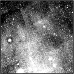
W4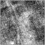

Figure 12: Effect of median-filtering input frames in W3 and W4. Top row: W3 images for tile 1384p454. The AllWISE Release Atlas Image (left) shows considerable structure, some of which clearly follows the input frame boundaries. I find visually similar artifacts if I omit the median filtering step (middle). Applying a median filter (right), the spatially varying background is essentially gone. Note the dark ring (suppressed background) around the bright star at the bottom of the frame. (The bright “star” at the middle-left is a persistence artifact from this bright source.) Bottom row: W4 images.

WISE	unWISE	unWISE	unWISE (no m.f.,
	(median filter)	(no median filter)	background matched)

Figure 13: Effect of median filtering in the presence of large, bright structures. This is part of tile 0098p408, containing M31. Left: The AllWISE image seems to show a slight depression in the background level above and right of the galaxy core. Second column: My unWISE median-filtered image has a severely depressed background level near the galaxy core, since the local median within the galaxy is very high. Third column: with median-filtering disabled, I get results similar to AllWISE. Right: with median-filtering off and background-matching on, the background looks smooth.

4 Discussion

The method presented here includes a number of heuristics to handle the imperfections in real data. These heuristics include noise estimation for image weighting; masked-pixel patching; background estimation; and masking of transients and defects in the imaging.

I weight each image in a coadd based on an estimate of an image-wide (scalar) noise estimate. I did not want to use pixel-wise error estimates (which incorporate a Poisson noise term from the source as well as the sky) since these lead to biased estimates (pixels with fewer counts get a smaller error estimate and hence more weight). Using an error estimate based only on the baseline background and read-noise should result in weights that optimize the detectability of faint (background-dominated) isolated point sources. I chose a simple heuristic for estimating this scalar error estimate: I take the median of the unmasked uncertainty pixels from the WISE single-frame pipeline. Since these uncertainty pixels include a component due to Poisson noise from the signal as well as read noise, the median value is slightly biased high. I could instead attempt to estimate the mode of the uncertainty distribution in the same way I estimate the background level.

Since I resample the input frames using the Lanczos kernel, masked pixels in the input images would lead to large holes (as large as the support of the kernel) in the resampled images. Since several percent of the pixels in typical WISE images are masked, this would have resulted in unacceptably large losses, so I chose to “patch” pixels. My crude approach is simply to average neighboring valid pixels. Other approaches for patching defects include the linear predictive filter used by the Sloan Digital Sky Survey (Stoughton et al., 2002). Patching pixels can be seen as redistributing the weights of the interpolation kernel from the masked pixel to its neighbors. I mask the resampled pixel closest to the patched pixel, so it is not included in the “masked” coadds, $C_{m}$. Nearby resampled pixels also include some contribution from the patched pixel; I chose to include these since their effect should be rather small. A more principled (but much more expensive) approach to patching images would be to fit a forward model to a small image patch and take the model prediction (with the model fit to unmasked pixels) as the patched pixel value. This would take into account the point-spread function, nearby sources, and many nearby pixels, resulting in predictions that were consistent with the modelled astrophysical scene.

For the W1 and W2 bands, I assume flat backgrounds and estimate a single scalar background level. For W3 and W4, I found it helpful to fit a varying background, and I chose to use a spatial median filter for this purpose. If I had a better model for the backgrounds (from astrophysical and instrumental sources) and could fit or marginalize over this model, that would comes closer to producing ideal coadds. A median filter should generally remove trends on spatial scales of order the filter size and preserve features smaller than the filter, but will introduce biases near bright sources and crowded regions; see Figure 13 for example. It would perhaps be better to avoid including in the median estimate any pixels that appear to be “contaminated” by sources (for example, by skipping pixels that are significantly different than their neighbors), though this is just a further heuristic rather than a real solution to the problem of estimating backgrounds. I am currently exploring possible approaches to reducing the highly depressed background level around bright structures (as shown in Figure 13). One option would be to also median-smooth on a larger spatial scale and add those filtered values back in, though this would likely still result in artifacts around structures in a range of scales. Another option would be to find the median or some other statistic of the stack of median-smoothed values, adding this back to the coadd. This way, extended structures that are consistent in many individual exposures would appear in the coadd. Yet another approach would be to match the large-scale variations to those found in other data sets, as done by Meisner et al. (2014); indeed, their maps, with point sources and other small-scale structures removed, could be ideal for repairing the large-scale structures damaged by my median filtering.

The AllWISE Atlas Images were created using a “background-matching” approach for removing frame-to-frame variations in the background level. In this approach, as a frame is being accumulated into the coadd, its median value is matched to that of the existing coadd, in the region where they overlap. This approach tends to produce backgrounds that are smooth on large scales (see Figure 13), even in the presence of bright objects, since it uses no explicit estimation of the background level. However, it has the disadvantages that it is order-dependent—the first few frames accumulated into the coadd have disproportionately large influence on the final background—and also depends on the extent of the coadd tile: shifting the tile boundaries results in different backgrounds.

I attempt to mask transients and defects in the individual exposures by building an initial coadd to estimate the mean and variance of the input frame pixels contributing to each coadd pixel. This approach of storing only summary statistics is in contrast to the approach used in the AllWISE Release, of keeping in memory the full list of input frame pixels contributing to each coadd pixel, and then performing operations on those pixel lists. Using robust statistical estimates, the WISE team’s approach should allow nearly 50% of the input frames to be contaminated without affecting the results. This power presumably comes at significant computational cost and complexity. My simpler and cheaper approach of accumulating only the mean and variance (and removing an input frame’s contribution to these estimates before evaluating that frame) should be expected to work well at flagging a single moderate outliers in each pixel, or multiple extreme outliers if the number of contributing frames is large. If there is more than a single outlier, the sample variance estimate will be inflated by the outlier, and moderate outliers will no longer deviate from the mean enough to be flagged. Despite these expected shortcomings, I have found that my simple approach seems to work well in practice. Possible improvements would be to detect pixels whose sample variance is larger than would be expected from a Poisson noise model, and do more careful outlier detection there.

In attempting to remove artifacts such as satellite trails and cosmic rays, we also remove fast-moving sources and clip sources that vary in brightness. One would expect variable sources to induce a larger sample variances than a non-varying source of the same mean magnitude, and this might be a simple way of flagging such sources. In general, though, these coadds should be used for the non-transient sky only.

One might ask why I felt it necessary to write a new code to produce these coadds when publicly available codes such as SWarp (Bertin et al., 2002) already exist. The core coaddition (image warping and interpolation) could indeed have been implemented using SWarp, but the detection and masking of transients and defects (which I do by creating first-round coadds) would have required first running SWarp to do the interpolation and first-round coadds, then detecting and masking transients in the “temporary” files written by SWarp, then running the second-round coadds on these altered files. I felt it would be simpler to reimplement the warping and interpolation functionality.

The WISE team should be commended on their timely, high-quality data releases. One shortcoming I have attempted to address in this work is that the Atlas Images are blurred by convolution by the point-spread function. I present a new set of coadded images that preserve the resolution of the original exposures. I use a theoretically justified resampling method with some approximations. In the process of validating my results, I found that my pixelwise sample variances, and likely the AllWISE Release Atlas Images as well, include a $\sim$3% systematic uncertainty in addition to the expected statistical uncertainty. These images, and the code used to produce them, are publicly available at http://unwise.me.

References

- Bertin et al. (2002) Bertin, E. et al., 2002, in ADASS XI, ASP Conference Series, 281, 228
- Fruchter and Hook (2002) Fruchter, A. S. and Hook, R. N., 2002, PASP, 144, 144
- Jerri (1977) Jerri, A. J., 1977, Proceedings of the IEEE, 65, 1565
- Lauer (1999) Lauer, T. R., 1999, PASP, 111, 227
- Lupton (2004) Lupton, R. H. et al., 2004, PASP, 116, 133
- Mahmounian and Wucknitz (2013) Mahmounian, H. and Wucknitz, O., 2013, arXiv:1307.4177
- Mainzer et al. (2011) Mainzer, A. et al., 2011, ApJ, 731, 53
- Masci and Fowler (2008) Masci, F. J. and Fowler, J. W., 2008, in ADASS XVIII, ASP Conference Series, 411, 67
- Meisner et al. (2014) Meisner, A. M. and Finkbeiner, D. P., 2014, ApJ, 781, 5
- Rowe et al. (2011) Rowe, B., Hirata, C. and Rhodes, J., 2011, ApJ, 741, 46
- Stoughton et al. (2002) Stoughton, C. et al., 2002, AJ, 123, 485
- Wright et al. (2010) Wright, E. L. et al., 2010, AJ, 140, 1868
- York et al. (2000) York, D. G. et al., 2000, AJ, 120, 1579