Consistency tests of the stability of fundamental couplings and unification scenarios
Abstract
We test the consistency of several independent astrophysical measurements of fundamental dimensionless constants. In particular, we compare direct measurements of the fine-structure constant and the proton-to-electron mass ratio (mostly in the optical/ultraviolet) with combined measurements of , and the proton gyromagnetic ratio (mostly in the radio band). We point out some apparent inconsistencies, which suggest that hidden systematics may be affecting some of the measurements. These findings demonstrate the importance of future more precise measurements with ALMA, ESPRESSO and ELT-HIRES. We also highlight some of the implications of the currently available measurements for fundamental physics, specifically for unification scenarios.
I Introduction
The stability of nature’s fundamental couplings is among the most profound open issues in astrophysics and fundamental physics, and has been identified by the European Space Agency (ESA) and the European Southern Observatory (ESO) as one of the key drivers for the next generation of ground and space-based facilities. While historically we have assumed that these are spacetime-invariant, this is only a simplifying assumption, whose only possible justification is an appeal to Occam’s razor.
Although we have no ’theory of couplings’, that describes their role in physical theories (or even which of them are really fundamental), at a phenomenological level it is well known that fundamental couplings run with energy, and in many extensions of the standard model they will also roll in time and ramble in space (ie, they will depend on the local environment). In particular, this will be the case in theories with additional spacetime dimensions, such as string theory. A detection of varying fundamental couplings will be revolutionary: it will automatically prove that the Einstein Equivalence Principle is violated and that there is a fifth force of nature. Reviews of the subject can be found in Martins (2002); Garcia-Berro et al. (2007); Uzan (2011).
One must also realize that even improved null results are important. Naively, the natural scale for cosmological evolution of one of these couplings (if one assumes that it is driven by a scalar field) would the Hubble time. We would therefore expect a drift rate of the order of yr-1. However, current local bounds coming from atomic clock comparison experiments Rosenband et al. (2008), are already about 6 orders of magnitude stronger, and rule out many otherwise viable dynamical dark energy models. A recent combined analysis of all currently available atomic clock measurements Ferreira et al. (2012) led to the following indirect 95% confidence intervals for present-day () drift rates
| (1) |
| (2) |
to be compared to the direct experimental result of Rosenband et al. (2008) for the fine-structure constant (also at the 95% confidence level)
| (3) |
Astrophysical measurements have led to claims for Murphy et al. (2004); Reinhold et al. (2006); Webb et al. (2011) and against Srianand et al. (2007); King et al. (2008); Thompson et al. (2009) variations of the fine-structure constant and the proton-to-electron mass ratio at redshifts . An ongoing Large Program at European Southern Observatory’s Very Large Telescope (henceforth referred to as the LP) is expected to clarify matters Molaro et al. (2013); Rahmani et al. (2013), but a resolution may have to wait for a forthcoming generation of high-resolution ultra-stable spectrographs such as ESPRESSO Pepe et al. (2014) and ELT-HIRES Maiolino et al. (2013); Pedrosa et al. (2013) which include improving these measurements among their key science goals (and in some cases this actually drives the instrument’s design). Answering this question is also essential in order to shed light on the enigma of dark energy Parkinson et al. (2004); Nunes and Lidsey (2004); Doran (2005); Amendola et al. (2012).
Any Grand-Unified model predicts a specific relation between the variation of and those of and other couplings, and therefore simultaneous measurements of both provide key consistency tests, with direct implications for the phenomenology of these models. The basic formalism for these tests was developed in Coc et al. (2007); Luo et al. (2011) (simpler, and somewhat more model-dependent studies were also done in Dent et al. (2009); Berengut et al. (2011)). This formalism has subsequently been applied to astrophysical observations of solar-type stars Vieira et al. (2012) and neutron stars Perez-Garcia and Martins (2012), as well as to local experiments with atomic clocks Ferreira et al. (2012). More recently we have also applied this formalism to observations of the radio source PKS1413135 Ferreira et al. (2013).
Here, we extend these previous analyses to a much broader set of astrophysical measurements of fundamental couplings. These measurements span a wide range of redshifts and were obtained with an equally diverse range of observational techniques, from the optical/UV to the radio band. We will simply take the various (independent) available measurements at face value and check for their internal consistency. Unless otherwise is stated, the results of these spectroscopic measurements will be presented in units of parts per million (ppm), ie. .
We note that in the present analysis we will be focusing on time variations, and for that reason we do not explicitly include the results of Webb et al. Webb et al. (2011), which provide some evidence for spatial variations, in our analysis. Extending our formalism to allow for possible spatial variations is possible in principle but it requires additional statistical analysis tools; for this reason, it is left for subsequent work.
II Phenomenological models
We shall work on the assumption that varying fundamental couplings are due to a dynamical, dilaton-type scalar field. In this section we describe the specific class of unification scenarios we will be considering, as well as the possible effects of couplings between this degree of freedom and photons (which can have relevant observational consequences). The required theoretical formalism has been described in our previous papers Ferreira et al. (2012, 2013); Avgoustidis et al. (2012, 2013) and in other references therein; here we will simply provide a brief summary.
II.1 Unification scenarios
We consider a class of grand unification models (in which unification happens at an unspecified high-energy scale) where the weak scale is determined by dimensional transmutation and the relative variation of all the Yukawa couplings is the same. We also assume that the variation of the couplings is driven by a dilaton-type scalar field (as in Campbell and Olive (1995)).
With these assumptions one finds that the variations of and are related via
| (4) |
where and are phenomenological (model-dependent) parameters, whose absolute values can be anything from order unity to several hundreds. Although physically one may expect them to be positive, for our purposes they can be taken as free parameters to be constrained by data. At a phenomenological level, the choice , can also describe the limiting case where varies but the masses don’t.
II.2 CMB temperature evolution
Overviews of the possible effects of scalar fields on the redshift evolution of the CMB temperature can be found in Avgoustidis et al. (2012, 2013). If there is a coupling between the scalar field and the radiation fluid, the photon temperature-redshift relation will be distorted away from its standard evolution. At a phenomenological level, this can be described with the additional parameter
| (7) |
with the available measurements of providing percent-level constraints Luzzi et al. (2009); Noterdaeme et al. (2011); Avgoustidis et al. (2012). The corresponding evolution of the radiation density is
| (8) |
with being the cosmological scale factor.
One specific example of such a class of phenomenological models is the Bekenstein-Sandvik-Barrow-Magueijo (BSBM) Sandvik et al. (2002), for which it has been shown Avgoustidis et al. (2013) that
| (9) |
In this specific case we have variations without corresponding variations of (as previously pointed out, in our formalism this can be described by the parameter choice , ). But regardless of the BSBM specific case, we can similarly take this as a phenomenological relation that can be tested observationally. There is currently no system for which both and have been measured, but such systems do exist for . In particular, Salumbides et al. (2012) points out that the band system of CO, which has been detected in six galaxies in the redshift range –, is a probe method for , while as already demonstrated in Noterdaeme et al. (2011) CO is also ideal to measure .
It is convenient to define the relative temperature variation
| (10) |
with the local () measurement being Mather et al. (1999)
| (11) |
With these definitions and the above results we have
| (12) |
and therefore
| (13) |
which provides a further consistency test.
III Current spectroscopic measurements
In this section we list the current astrophysical measurements that we will be using in our analysis. (As previously mentioned, we’ll usually list them in units of parts per million.) This is not meant to be a ’historical’ review listing all available measurements. In most cases we use only the tightest available measurement for each astrophysical source. A few older measurements along other lines of sight have not been used, on the grounds that they would have no statistical weight in our analysis. Nevertheless, we will include some low-sensitivity but high-redshift measurements, as these are illustrative of the redshift range that may be probed by future facilities. Our two exceptions regarding measurements of the same source concern
-
•
Measurements using different (that is, independent) techniques—typically, measurements of or combined measurements using different molecules, and
-
•
Measurements obtained with different spectrographs .
| Object | z | Ref. | ||
| PKS1413135 | 0.247 | Kanekar et al. (2010) | ||
| PKS1413135 | 0.247 | Darling (2004) | ||
| PKS1413135 | 0.247 | Murphy et al. (2001) | ||
| B0218357 | 0.685 | Murphy et al. (2001) | ||
| J01340931 | 0.765 | Kanekar et al. (2012) | ||
| J23581020 | 1.173 | Rahmani et al. (2012) | ||
| J16230718 | 1.336 | Rahmani et al. (2012) | ||
| J23400053 | 1.361 | Rahmani et al. (2012) | ||
| J05010159 | 1.561 | Rahmani et al. (2012) | ||
| J09110551 | 2.796 | Weiss et al. (2012) | ||
| J13373152 | 3.174 | Srianand et al. (2010) | ||
| BR12020725 | 4.695 | Lentati et al. (2013) | ||
| J09185142 | 5.245 | Levshakov et al. (2012) | ||
| J11485251 | 6.420 | Lentati et al. (2013) |
Table 1 contains current joint measurements of several couplings. Note that for the radio source PKS1413135 the three available measurements are sufficient to yield individual constraints on the variations of the three quantities at redshift . This was done in Ferreira et al. (2013), which at the one-sigma (68.3) confidence level obtained
| (14) |
| (15) |
| (16) |
| Object | z | Spectrograph | Ref. | |
|---|---|---|---|---|
| HE05154414 | 1.15 | UVES | Molaro et al. (2008) | |
| HE05154414 | 1.15 | HARPS/UVES | Chand et al. (2006) | |
| HE00012340 | 1.58 | UVES | Agafonova et al. (2011) | |
| HE22172818 | 1.69 | UVES-LP | Molaro et al. (2013) | |
| Q1101264 | 1.84 | UVES | Molaro et al. (2008) |
Table 2 contains individual measurements. Conservatively we only list measurements where data was acquired specifically for this purpose—but these are, in many cases, the ones with the smallest uncertainties. In particular, the measurement listed in bold, towards HE22172818, comes from the ongoing LP and is, arguably, the one with the most robust control of systematics (the quoted error bar includes both statistical and systematic uncertainties, added in quadrature).
| Object | z | Method | Ref. | |
| B0218357 | 0.685 | // | Murphy et al. (2008) | |
| B0218357 | 0.685 | // | Kanekar (2011) | |
| PKS1830211 | 0.886 | / | Henkel et al. (2009) | |
| PKS1830211 | 0.886 | Ilyushin et al. (2012) | ||
| PKS1830211 | 0.886 | Muller et al. (2011) | ||
| PKS1830211 | 0.886 | Bagdonaite et al. (2013) | ||
| J2123005 | 2.059 | / (VLT) | van Weerdenburg et al. (2011) | |
| J2123005 | 2.059 | / (Keck) | Malec et al. (2010) | |
| HE00271836 | 2.402 | Rahmani et al. (2013) | ||
| Q2348011 | 2.426 | Bagdonaite et al. (2012) | ||
| Q0405443 | 2.597 | King et al. (2008) | ||
| J0643504 | 2.659 | Albornoz Vásquez et al. (2014) | ||
| Q0528250 | 2.811 | / | King et al. (2011) | |
| Q0347383 | 3.025 | Wendt and Reimers (2008) |
Table 3 contains individual measurements. Note that several different molecules can be used (with ammonia being the most common at low redshift and molecular hydrogen at high redshift), and in the case of the gravitational lens PKS1830211 several independent measurements exist. The tightest available constraint was obtained in this system, from observations of methanol transitions Bagdonaite et al. (2013). On the other hand, two very recent publications containing measurements along the line of sight towards J0643504 both suggest variations, though at different levels of significance. We have listed the more conservative one, from Albornoz Vásquez et al. (2014) on the table; for comparison Bagdonaite et al. (2014) finds ppm. The measurement in bold, towards HE00271836, again comes from the ongoing LP.
| Object | z | (ppm) | Ref. | (K) | Ref. | |
|---|---|---|---|---|---|---|
| PKS1830-211 | 0.886 | Bagdonaite et al. (2013) | Muller et al. (2013) | |||
| Q0347-383 | 3.025 | Wendt and Reimers (2008) | Molaro et al. (2002) |
Finally, Table 4 contains the systems with both and measurements, as well as the corresponding relative temperature variation defined in Eq. (10). Clearly, these measurements have relatively large uncertainties and therefore currently have no significant additional constraining power. However, we include them here as a proof of concept, since the significantly better sensitivity of ALMA and ELT-HIRES is expected to improve both the quantity and the accuracy of these measurements.
IV Analysis
We now proceed to describe several different consistency studies. In each case we will mainly focus on the consistency of each set of measurements, but we will also provide a brief discussion of what these correspond to in terms of constraints in the phenomenological unification plane.
IV.1 Self-consistency
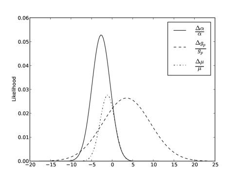
We will start by obtaining the individual values for , and derived from the measurements in Table 1. In doing this we will be neglecting a possible redshift-dependence of the variations; this is of course an approximation, but given the small number of available measurements (and the large uncertainties in some of them) it is a legitimate exercise. With better data the exercise could be separately done for different redshift bins. Indeed, the present analysis is an extension of a previous analysis Ferreira et al. (2013) where we only looked at the three measurements at . Figure 1 shows the 1D likelihood contours for each of these parameters. At the one-sigma () confidence level we find
| (17) |
| (18) |
| (19) |
and at the two-sigma level all are consistent with no variations. Notice the significantly smaller uncertainties as compared to the results of Eq. (14–16) for the source at alone: the one-sigma uncertainties on , and are respectively reduced by factors of about 20, 22 and 15. Cpmparing these results with those listed in Tables 2 and 3 we also note that the values of and are consistent with those found by the LP, but not with some of the other measurements in Tables 2-3 (or with Bagdonaite et al. (2014)).
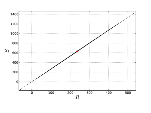
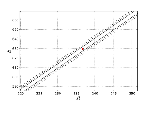
By using the relations discussed in Sect. II we can also translate the measurements of Table 1 into constraints on the plane. These are shown in Fig. 2. As in previous analyses Ferreira et al. (2012, 2013) there is a clear degeneracy direction: in other words, these measurements constrain a particular combination of the phenomenological parameters and . It’s also straightforward to determine the one-dimensional confidence intervals for and ; at the one-sigma confidence level we find
| (20) |
| (21) |
these are fairly similar to the ones we found in Ferreira et al. (2013) for the three measurements towards PKS1413135, showing that these carry a significant weight in the overall analysis.
IV.2 Additional measurements
The data in table 1 can also be analyzed assuming one of the direct measurements in Table 2. This will provide constraints on the plane as well as on the plane.
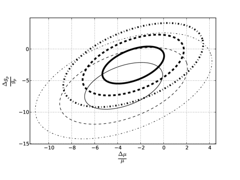
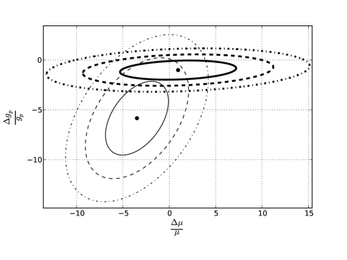
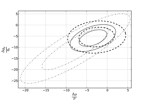
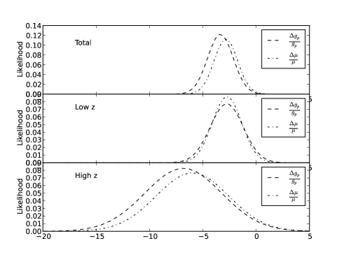
Figure 3 shows relevant contours in the , using either the best measurement (by which we mean the one with the smallest uncertainty, that is Molaro et al. (2008)) or the LP measurement Molaro et al. (2013): this is useful to provide intuition on how these combined analyses depend on the choice of (in this case) . As expected, having an measurement with a smaller uncertainty leads to tighter constraints on the individual parameters. We will now use the LP result as the ’baseline’ measurement.
Note also that the degeneracy direction in this plane is different from that coming from current atomic clock measurements; this is illustrated in Fig. 4. In order to make this comparison we must make the atomic clock results dimensionless, and the simplest way to achieve this is to multiply them by the present Hubble time, . Thus the plot effectively compares astrophysical measurements of with laboratory measurements of . Although the resulting comparison is illuminating, one should bear in mind that no realistic model is expected to have a variation of the couplings that is linear in time from to , and therefore this rescaling by the Hubble time is somewhat simplistic.
| Sample | (ppm) | (ppm) |
|---|---|---|
| Full |
On the other hand, Fig. 5 displays constraints obtained by dividing the full sample into two equal-sized sub-samples, according to redshift: the transition will thus be at . As expected, tighter and less degenerate constraints can be obtained at low redshift, but note also that the likelihood contours have different degeneracy directions at high and low redshifts. This stems from the fact that different measurement techniques probe different combinations of couplings, and each technique typically has a limited range of redshifts over which it can be used (due to target availability or other practicalities).
Fig. 6 shows relevant one-dimensional likelihoods for the full sample and the two subsamples. This leads to the 1D confidence intervals listed (at one sigma) in Table 5 for the full sample and the subsamples. Interestingly both are non-zero (and negative) at about the one to two sigma level.
These results can be compared with those found in the previous subsection, and the 1D constraints on can also be checked for consistency against the direct measurements in Table 3. One finds that in the case of there is no strong disagreement, except in the case of the measurement in Bagdonaite et al. (2014) which is a strong detection with opposite sign. On the other hand, there is some tension between the values in Table 5 and those inferred in the analysis in section IV.A: the analysis of the present section indicates a negative variation of at more than two sigma.
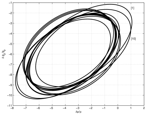
Naturally, most of the signal for the above detections comes from the two measurements in Murphy et al. (2008); Weiss et al. (2012). This can be easily confirmed, as summarized in Fig. 7: by redoing the analysis while removing one measurement at a time, we see that the results are significantly different (and much closer to null) when either of these measurements is removed, while they change very little if one of the others is removed.
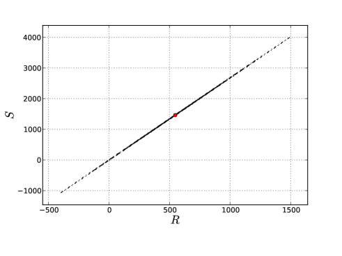
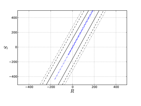
The top panel of fig. 8 shows the derived constraints on the – plane, still assuming the LP measurement in Table 2. Comparing this with the corresponding analysis in section IV.A, we notice that although the degeneracy direction is maintained, both the best-fit values and the corresponding uncertainties increase. Specifically, we now find at the one-sigma () confidence level
| (22) |
| (23) |
Nevertheless, the two sets of parameters are consistent within their error bars. While the relevance of these numbers is at present unclear given the limitations of the currently available data, these results are encouraging in the sense that they show that this is potentially a very sensitive probe of unification, with may come to fruition with the next generation of facilities. It is also interesting to compare these results with touse obtained in Ferreira et al. (2012) for the atomic clock measurements (at ); this is done in the bottom panel of fig. 8. One notices that the degeneracy direction of both constraints is almost (though not exactly) the same, while the region of the parameter space allowed by atomic clock measurements (which are all null results) is significantly wider.
IV.3 Additional measurements
A similar analysis can be done with : data in Table 1 can be analyzed assuming one or more of the measurements in Table 3. Naturally this will now provide constraints on the plane, which can also be compared with the results of the previous subsections, and the constraints on can then be checked for consistency against the direct measurements in table 2, and with the results form the Webb dipole Webb et al. (2011).
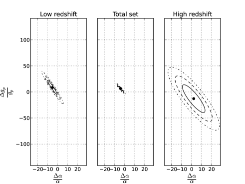
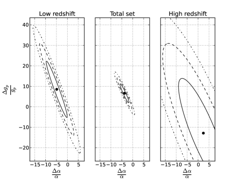
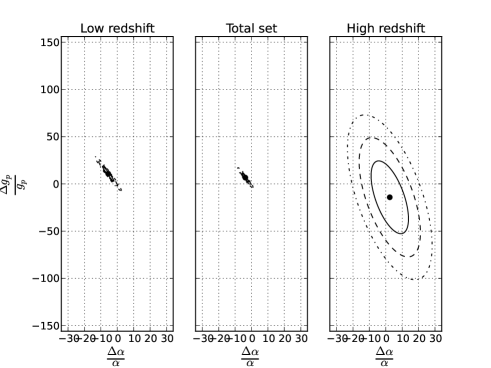
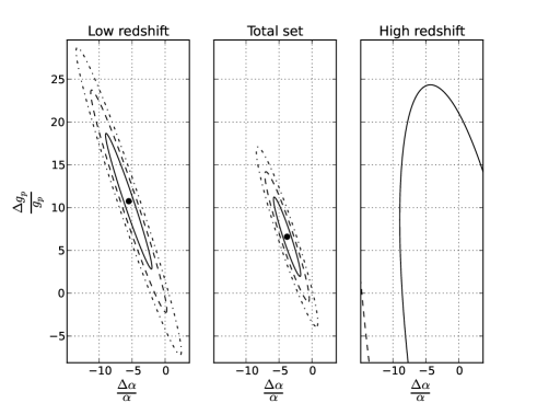
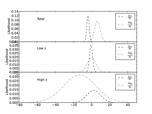
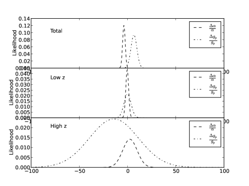
In this case we will also split the sample into two subsamples according to redshift, using as baseline measurements the Methanol one Bagdonaite et al. (2013) for the low redshift subsample and the LP one Rahmani et al. (2013) for the high redshift subsample. The results of this analysis are shown in Figs. 9 and 10. In the former the separation between low and high redshift is set at redshift , while in the latter it is set at . Here again stronger constraints can be obtained at low redshift. Fig. 11 shows relevant 1D likelihoods for the full sample and the two subsamples, while the corresponding 1D confidence intervals are listed (at one sigma) in Table 6.
| Sample | (ppm) | (ppm) |
|---|---|---|
| Full |
Here the results are somewhat interesting: at low redshifts these datasets prefer a slightly negative value of and a slightly positive value of , although in each case this is a less than two sigma effect. The former is consistent with the analysis of Sect. IV.A and (at two sigma) not inconsistent with the direct measurements in Table 2, while the latter is inconsistent with what we found in Sect. IV.B (where a negative variation of was preferred).
IV.4 Comparing the various analyses
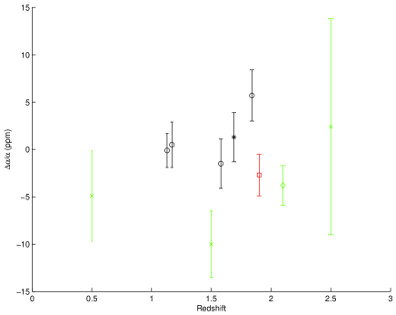
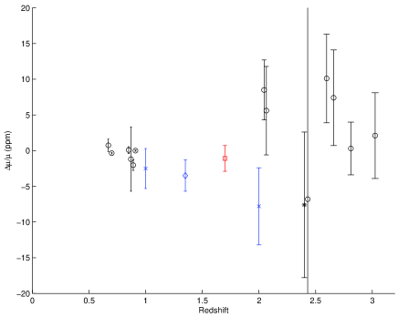
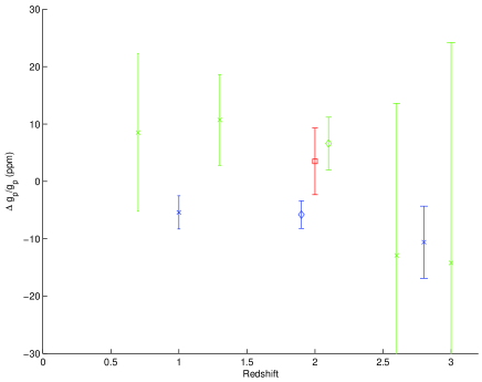
Fig. 12 presents a brief visual summary of our derived results for , and and compares them with the direct measurements of and . We emphasize that the placing of these inferred measurements at particular redshifts is purely indicative, since they are the result of combining direct measurements at various different redshifts. (Still, this is useful for comparison purposes.)
We note that at low redshifts the indirect determinations of tend to lead to slightly smaller results than the direct ones, while that is not the case for . Somewhat more noticeable is the fact that the various methods we used to obtain bounds on —either from the data of Table 1, or combining these measurements with direct measurements of or —lead to quite different results.
These inconsistencies suggest that the uncertainties in some of the measurements may be underestimated, possibly due to the presence of hidden systematics. While a discussion of the source of these systematics is beyond the scope of the present work, we refer the reader to two of the recent LP publications Molaro et al. (2013); Rahmani et al. (2013), where the issue is discussed in considerable detail.
V Conclusions
We have carried out some simple consistency tests of various recent astrophysical measurements of dimensionless fundamental couplings. Direct measurements of the fine-structure constant and the proton-to-electron mass ratio can be obtained, mostly in the optical/ultraviolet, from a range of absorption systems, typically above redshift and up to . At lower redshifts, on the other hand, various combinations of , and the proton gyromagnetic ratio can be measured, usually in the radio band. The goal of our analysis was to provide a basic comparison between the two types of measurements.
When attempting such comparisons, previous authors often dealt with combined measurements of , and by assuming that only one of these couplings varies (thus turning the combined measurement into one of the coupling in question). This assumption is not justified, in the obvious sense that it does not hold for the vast majority of realistic models. In our analysis the three couplings were allowed to vary simultaneously, and the datasets were used to obtain the most likely values in this parameter space. This somewhat phenomenological approach allows us to compare measurements at various different redshifts, in an approximate but model-independent way.
Naturally a different approach could be taken: one can always choose a specific model (for which the redshift dependence of the couplings will be fully determined), and then compare measurements at different redshifts in the context of this model. This may potentially lead to tighter contraints, though naturally they will be model-dependent. Given the limitations (in quantity and arguably also quality) of the currently available data, we think that a phenomenological approach is more fruitful.
From our analysis it is clear that there are some apparent inconsistencies in the determinations of the various couplings. This is particularly the case in the various indirect determinations of . These results support the expectation that hidden systematics may be affecting some of the measurements. Trying to improve this state of affairs is af course the main goal of the ongoing UVES Large Program for Testing Fundamental Physics Molaro et al. (2013); Rahmani et al. (2013).
We must also stress that measurements of various combinations , and , as well as individual measurements of and in the same system, are particularly useful. Any Grand-Unified scenario predicts specific (model-dependent) relations between the variations of , and . Thus simultaneous measurements of several of these can provide key consistency tests, which will complement (and in some sense are more fundamental than) those that can be done in particle accelerators. Following previous work Ferreira et al. (2012, 2013), we have briefly illustrated this for the particular class of models previously considered in Coc et al. (2007); Luo et al. (2011), but with suitable generalizations this may be applicable to any unification scenario which includes varying couplings.
Looking further ahead, our results demonstrate the importance of future more precise astrophysical measurements of the stability of these couplings. These future datasets will also make detailed model comparisons possible, including those allowing for spatial or environmental dependencies which may have distinctive signatures Silva et al. (2014). Fortunately, forthcoming facilities such as ALMA and the ESPRESSO and ELT-HIRES spectrographs (at the VLT and E-ELT, respectively), with higher sensitivity and a better control over possible systematics, will provide a detailed and much more accurate mapping of the behaviour of these couplings up to redshift —and possibly well beyond.
Acknowledgements.
We are grateful to Mariana Julião for useful discussions in the early stages of this work. This work was done in the context of the project PTDC/FIS/111725/2009 from FCT (Portugal). O.F. and J.S. acknowledge financial support from Programa Joves i Ciència, funded by Fundació Catalunya–La Pedrera. C.J.M. is also supported by an FCT Research Professorship, contract reference IF/00064/2012, funded by FCT/MCTES (Portugal) and POPH/FSE (EC).References
- Martins (2002) C. J. A. P. Martins, Phil.Trans.Roy.Soc.Lond. A360, 2681 (2002), arXiv:astro-ph/0205504 [astro-ph] .
- Garcia-Berro et al. (2007) E. Garcia-Berro, J. Isern, and Y. A. Kubyshin, Astron.Astrophys.Rev. 14, 113 (2007).
- Uzan (2011) J.-P. Uzan, Living Rev.Rel. 14, 2 (2011), arXiv:1009.5514 [astro-ph.CO] .
- Rosenband et al. (2008) T. Rosenband, D. B. Hume, P. O. Schmidt, C. W. Chou, A. Brusch, L. Lorini, W. H. Oskay, R. E. Drullinger, T. M. Fortier, J. E. Stalnaker, S. A. Diddams, W. C. Swann, N. R. Newbury, W. M. Itano, D. J. Wineland, and J. C. Bergquist, Science 319, 1808 (2008).
- Ferreira et al. (2012) M. C. Ferreira, M. D. Julião, C. J. A. P. Martins, and A. M. R. V. L. Monteiro, Phys.Rev. D86, 125025 (2012), arXiv:1212.4164 [hep-ph] .
- Murphy et al. (2004) M. T. Murphy et al., Lect. Notes Phys. 648, 131 (2004), arXiv:astro-ph/0310318 .
- Reinhold et al. (2006) E. Reinhold, R. Buning, U. Hollenstein, A. Ivanchik, P. Petitjean, et al., Phys.Rev.Lett. 96, 151101 (2006).
- Webb et al. (2011) J. K. Webb, J. A. King, M. T. Murphy, V. V. Flambaum, R. F. Carswell, et al., Phys.Rev.Lett. 107, 191101 (2011), arXiv:1008.3907 [astro-ph.CO] .
- Srianand et al. (2007) R. Srianand, H. Chand, P. Petitjean, and B. Aracil, Phys. Rev. Lett. 99, 239002 (2007).
- King et al. (2008) J. A. King, J. K. Webb, M. T. Murphy, and R. F. Carswell, Phys. Rev. Lett. 101, 251304 (2008), arXiv:0807.4366 [astro-ph] .
- Thompson et al. (2009) R. I. Thompson et al., Astrophys. J. 703, 1648 (2009), arXiv:0907.4392 [astro-ph.CO] .
- Molaro et al. (2013) P. Molaro, M. Centurion, J. Whitmore, T. Evans, M. Murphy, et al., A. & A. 555, A68 (2013), arXiv:1305.1884 [astro-ph.CO] .
- Rahmani et al. (2013) H. Rahmani, M. Wendt, R. Srianand, P. Noterdaeme, P. Petitjean, P. Molaro, J. B. Whitmore, M. T. Murphy, M. Centurion, H. Fathivavsari, S. D’Odorico, T. M. Evans, S. A. Levshakov, S. Lopez, C. J. A. P. Martins, D. Reimers, and G. Vladilo, MNRAS 435, 861 (2013), arXiv:1307.5864 [astro-ph.CO] .
- Pepe et al. (2014) F. Pepe, P. Molaro, S. Cristiani, R. Rebolo, N. C. Santos, H. Dekker, D. Mégevand, F. M. Zerbi, A. Cabral, P. Di Marcantonio, M. Abreu, M. Affolter, M. Aliverti, C. Allende Prieto, M. Amate, G. Avila, V. Baldini, P. Bristow, C. Broeg, R. Cirami, J. Coelho, P. Conconi, I. Coretti, G. Cupani, V. D’Odorico, V. De Caprio, B. Delabre, R. Dorn, P. Figueira, A. Fragoso, S. Galeotta, L. Genolet, R. Gomes, J. I. González Hernández, I. Hughes, O. Iwert, F. Kerber, M. Landoni, J.-L. Lizon, C. Lovis, C. Maire, M. Mannetta, C. Martins, M. Monteiro, A. Oliveira, E. Poretti, J. L. Rasilla, M. Riva, S. Santana Tschudi, P. Santos, D. Sosnowska, S. Sousa, P. Spanó, F. Tenegi, G. Toso, E. Vanzella, M. Viel, and M. R. Zapatero Osorio, Astronomische Nachrichten 335, 8 (2014).
- Maiolino et al. (2013) R. Maiolino, M. Haehnelt, M. Murphy, D. Queloz, L. Origlia, et al., (2013), arXiv:1310.3163 [astro-ph.IM] .
- Pedrosa et al. (2013) P. O. J. Pedrosa, A. C. O. Leite, and C. J. A. P. Martins, (2013), arXiv:1309.7770 [astro-ph.CO] .
- Parkinson et al. (2004) D. Parkinson, B. A. Bassett, and J. D. Barrow, Phys.Lett. B578, 235 (2004), arXiv:astro-ph/0307227 [astro-ph] .
- Nunes and Lidsey (2004) N. J. Nunes and J. E. Lidsey, Phys.Rev. D69, 123511 (2004), arXiv:astro-ph/0310882 [astro-ph] .
- Doran (2005) M. Doran, JCAP 0504, 016 (2005), arXiv:astro-ph/0411606 [astro-ph] .
- Amendola et al. (2012) L. Amendola, A. C. O. Leite, C. J. A. P. Martins, N. J. Nunes, P. O. J. Pedrosa, and A. Seganti, Phys.Rev. D86, 063515 (2012), arXiv:1109.6793 [astro-ph.CO] .
- Coc et al. (2007) A. Coc, N. J. Nunes, K. A. Olive, J.-P. Uzan, and E. Vangioni, Phys.Rev. D76, 023511 (2007), arXiv:astro-ph/0610733 [astro-ph] .
- Luo et al. (2011) F. Luo, K. A. Olive, and J.-P. Uzan, Phys.Rev. D84, 096004 (2011), arXiv:1107.4154 [hep-ph] .
- Dent et al. (2009) T. Dent, S. Stern, and C. Wetterich, Phys.Rev. D79, 083533 (2009), arXiv:0812.4130 [hep-ph] .
- Berengut et al. (2011) J. Berengut, V. Flambaum, J. King, S. Curran, and J. Webb, Phys.Rev. D83, 123506 (2011), arXiv:1009.0591 [astro-ph.CO] .
- Vieira et al. (2012) J. P. P. Vieira, C. J. A. P. Martins, and M. J. P. F. G. Monteiro, Phys.Rev. D86, 043003 (2012), arXiv:1206.3665 [astro-ph.SR] .
- Perez-Garcia and Martins (2012) M. A. Perez-Garcia and C. J. A. P. Martins, Phys.Lett. B718, 241 (2012), arXiv:1203.0399 [astro-ph.CO] .
- Ferreira et al. (2013) M. C. Ferreira, M. D. Juli o, C. J. A. P. Martins, and A. M. R. V. L. Monteiro, Phys.Lett. B724, 1 (2013), arXiv:1305.7515 [astro-ph.CO] .
- Avgoustidis et al. (2012) A. Avgoustidis, G. Luzzi, C. J. A. P. Martins, and A. M. R. V. L. Monteiro, JCAP 1202, 013 (2012), arXiv:1112.1862 [astro-ph.CO] .
- Avgoustidis et al. (2013) A. Avgoustidis, C. J. A. P. Martins, A. M. R. V. L. Monteiro, P. E. Vielzeuf, and G. Luzzi, (2013), arXiv:1305.7031 [astro-ph.CO] .
- Campbell and Olive (1995) B. A. Campbell and K. A. Olive, Phys.Lett. B345, 429 (1995), arXiv:hep-ph/9411272 [hep-ph] .
- Flambaum and Tedesco (2006) V. Flambaum and A. Tedesco, Phys.Rev. C73, 055501 (2006), arXiv:nucl-th/0601050 [nucl-th] .
- Flambaum et al. (2004) V. Flambaum, D. B. Leinweber, A. W. Thomas, and R. D. Young, Phys.Rev. D69, 115006 (2004), arXiv:hep-ph/0402098 [hep-ph] .
- Luzzi et al. (2009) G. Luzzi, M. Shimon, L. Lamagna, Y. Rephaeli, M. De Petris, et al., Astrophys.J. 705, 1122 (2009), arXiv:0909.2815 [astro-ph.CO] .
- Noterdaeme et al. (2011) P. Noterdaeme, P. Petitjean, R. Srianand, C. Ledoux, and S. López, A. & A. 526, L7 (2011), arXiv:1012.3164 [astro-ph.CO] .
- Sandvik et al. (2002) H. B. Sandvik, J. D. Barrow, and J. Magueijo, Phys.Rev.Lett. 88, 031302 (2002), arXiv:astro-ph/0107512 [astro-ph] .
- Salumbides et al. (2012) E. Salumbides, M. Niu, J. Bagdonaite, N. de Oliveira, D. Joyeux, et al., Phys.Rev. A86, 022510 (2012), arXiv:1208.4715 [physics.atom-ph] .
- Mather et al. (1999) J. C. Mather, D. Fixsen, R. Shafer, C. Mosier, and D. Wilkinson, Astrophys.J. 512, 511 (1999), arXiv:astro-ph/9810373 [astro-ph] .
- Kanekar et al. (2010) N. Kanekar, J. N. Chengalur, and T. Ghosh, Ap.J.Lett. 716, L23 (2010), arXiv:1004.5383 [astro-ph.CO] .
- Darling (2004) J. Darling, Astrophys.J. 612, 58 (2004), arXiv:astro-ph/0405240 [astro-ph] .
- Murphy et al. (2001) M. Murphy, J. Webb, V. Flambaum, M. Drinkwater, F. Combes, et al., Mon.Not.Roy.Astron.Soc. 327, 1244 (2001), arXiv:astro-ph/0101519 [astro-ph] .
- Kanekar et al. (2012) N. Kanekar, G. I. Langston, J. T. Stocke, C. L. Carilli, and K. M. Menten, Ap.J.Lett. 746, L16 (2012), arXiv:1201.3372 [astro-ph.CO] .
- Rahmani et al. (2012) H. Rahmani, R. Srianand, N. Gupta, P. Petitjean, P. Noterdaeme, and D. A. Vásquez, MNRAS 425, 556 (2012), arXiv:1206.2653 [astro-ph.CO] .
- Weiss et al. (2012) A. Weiss, F. Walter, D. Downes, C. Carrili, C. Henkel, et al., Astrophys.J. 753, 102 (2012), arXiv:1204.5614 [astro-ph.CO] .
- Srianand et al. (2010) R. Srianand, N. Gupta, P. Petitjean, P. Noterdaeme, and C. Ledoux, MNRAS 405, 1888 (2010), arXiv:1002.4620 [astro-ph.CO] .
- Lentati et al. (2013) L. Lentati, C. Carilli, P. Alexander, R. Maiolino, R. Wang, P. Cox, D. Downes, R. McMahon, K. M. Menten, R. Neri, D. Riechers, J. Wagg, F. Walter, and A. Wolfe, MNRAS , 721 (2013), arXiv:1211.3316 [astro-ph.CO] .
- Levshakov et al. (2012) S. A. Levshakov, F. Combes, F. Boone, I. I. Agafonova, D. Reimers, and M. G. Kozlov, A. & A. 540, L9 (2012), arXiv:1203.3649 [astro-ph.CO] .
- Molaro et al. (2008) P. Molaro, D. Reimers, I. I. Agafonova, and S. A. Levshakov, European Physical Journal Special Topics 163, 173 (2008), arXiv:0712.4380 .
- Chand et al. (2006) H. Chand, R. Srianand, P. Petitjean, B. Aracil, R. Quast, and D. Reimers, A. & A. 451, 45 (2006), arXiv:astro-ph/0601194 .
- Agafonova et al. (2011) I. I. Agafonova, P. Molaro, S. A. Levshakov, and J. L. Hou, A. & A. 529, A28 (2011), arXiv:1102.2967 [astro-ph.CO] .
- Murphy et al. (2008) M. T. Murphy, V. V. Flambaum, S. Muller, and C. Henkel, Science 320, 1611 (2008), arXiv:0806.3081 [astro-ph] .
- Kanekar (2011) N. Kanekar, Astrophys.J. 728, L12 (2011), arXiv:1101.4029 [astro-ph.CO] .
- Henkel et al. (2009) C. Henkel, K. M. Menten, M. T. Murphy, N. Jethava, V. V. Flambaum, J. A. Braatz, S. Muller, J. Ott, and R. Q. Mao, A. & A. 500, 725 (2009), arXiv:0904.3081 [astro-ph.CO] .
- Ilyushin et al. (2012) V. V. Ilyushin, P. Jansen, M. G. Kozlov, S. A. Levshakov, I. Kleiner, W. Ubachs, and H. L. Bethlem, Phys.Rev. A85, 032505 (2012), arXiv:1201.2090 [chem-ph] .
- Muller et al. (2011) S. Muller, A. Beelen, M. Guélin, S. Aalto, J. H. Black, F. Combes, S. J. Curran, P. Theule, and S. N. Longmore, A. & A. 535, A103 (2011), arXiv:1104.3361 [astro-ph.CO] .
- Bagdonaite et al. (2013) J. Bagdonaite, P. Jansen, C. Henkel, H. L. Bethlem, K. M. Menten, and W. Ubachs, Science 339, 46 (2013).
- van Weerdenburg et al. (2011) F. van Weerdenburg, M. Murphy, A. Malec, L. Kaper, and W. Ubachs, Phys.Rev.Lett. 106, 180802 (2011), arXiv:1104.2969 [astro-ph.CO] .
- Malec et al. (2010) A. L. Malec, R. Buning, M. T. Murphy, N. Milutinovic, S. L. Ellison, J. X. Prochaska, L. Kaper, J. Tumlinson, R. F. Carswell, and W. Ubachs, MNRAS 403, 1541 (2010), arXiv:1001.4078 [astro-ph.CO] .
- Bagdonaite et al. (2012) J. Bagdonaite, M. T. Murphy, L. Kaper, and W. Ubachs, MNRAS 421, 419 (2012), arXiv:1112.0428 [astro-ph.CO] .
- Albornoz Vásquez et al. (2014) D. Albornoz Vásquez, H. Rahmani, P. Noterdaeme, P. Petitjean, R. Srianand, and C. Ledoux, A. & A. 562, A88 (2014).
- King et al. (2011) J. A. King, M. T. Murphy, W. Ubachs, and J. K. Webb, MNRAS 417, 3010 (2011), arXiv:1106.5786 [astro-ph.CO] .
- Wendt and Reimers (2008) M. Wendt and D. Reimers, Eur.Phys.J.ST 163, 197 (2008), arXiv:0802.1160 [astro-ph] .
- Bagdonaite et al. (2014) J. Bagdonaite, W. Ubachs, M. T. Murphy, and J. B. Whitmore, Astrophys. J. 782, 10 (2014), arXiv:1308.1330 [astro-ph.CO] .
- Muller et al. (2013) S. Muller, A. Beelen, J. H. Black, S. J. Curran, C. Horellou, S. Aalto, F. Combes, M. Guélin, and C. Henkel, A. & A. 551, A109 (2013), arXiv:1212.5456 [astro-ph.CO] .
- Molaro et al. (2002) P. Molaro, S. A. Levshakov, M. Dessauges-Zavadsky, and S. D’Odorico, A. & A. 381, L64 (2002), arXiv:astro-ph/0111589 .
- Silva et al. (2014) M. F. Silva, H. A. Winther, D. F. Mota, and C. J. A. P. Martins, Phys.Rev. D89, 024025 (2014), arXiv:1310.2152 [astro-ph.CO] .