Finite Amplitude Method for Charge-Changing Transitions
in Axially-Deformed Nuclei

Abstract

We describe and apply a version of the finite amplitude method for obtaining the charge-changing nuclear response in the quasiparticle random phase approximation. The method is suitable for calculating strength functions and beta-decay rates, both allowed and forbidden, in axially-deformed open-shell nuclei. We demonstrate the speed and versatility of the code through a preliminary examination of the effects of tensor terms in Skyrme functionals on beta decay in a set of spherical and deformed open-shell nuclei. Like the isoscalar pairing interaction, the tensor terms systematically increase allowed beta-decay rates. This finding generalizes previous work in semimagic nuclei and points to the need for a comprehensive study of time-odd terms in nuclear density functionals.

I Introduction

Beta decay is an important process at the intersection of nuclear physics, astrophysics, and particle physics. The rapid neutron-capture process ($r$ process) proceeds through neutron-rich nuclei, the beta-decay rates for which determine final abundance distributions. The significance of the reactor neutrino anomaly for exotic new neutrino physics depends on forbidden beta-decay rates in neutron-rich fission products Hayes et al. (2013). In both these cases, the important rates are difficult or impossible to measure; we need to be able to calculate them instead.

The random-phase approximation (RPA) and its generalization, the quasiparticle random-phase approximation (QRPA), nowadays typically used in conjunction with Skyrme energy-density functionals (EDFs), are established tools for treating nuclear excitations. The matrix version of the charge-changing (or “pn”) Skyrme QRPA has been applied with some success in spherical nuclei. When the rotational symmetry of the mean field is broken, however, the dimension of the mean-field two-quasiparticle basis increases by orders of magnitude and the QRPA matrix becomes too large to fit in the main memory of a typical computer without aggressive truncation. Even then, supercomputing is needed to solve the equations. We have constructed a deformed matrix Skyrme pnQRPA program Mustonen and Engel (2013) from the code reported in Ref. Terasaki and Engel (2011) but cannot use it in reasonable amounts of computing time.

The finite amplitude method (FAM) is a much more efficient scheme for finding the linear response. Ref. Nakatsukasa et al. (2007) first proposed the method and Ref. Inakura et al. (2009) quickly applied it to obtain the RPA response in spherical and deformed nuclei. Ref. Avogadro and Nakatsukasa (2011) generalized the approach to the QRPA, and Ref. Stoitsov et al. (2011) applied the generalization to monopole transitions. In this article, we further extend the FAM to charge-changing QRPA transitions of arbitrary intrinsic angular momentum projection $K$ in deformed nuclei. We call the resulting approach the Skyrme proton-neutron finite amplitude method (pnFAM).

To illustrate the method, we examine the effects of Skyrme’s tensor terms on beta-decay rates. Minato and Bai Minato and Bai (2013) observed that a tensor interaction can reduce beta decay half-lives of magic and semi-magic nuclei considerably, bringing them into closer accord with experiment. If a similar reduction takes place in deformed nuclei, it might make it impossible to include an isoscalar pairing interaction without underpredicting half-lives. On the other hand, it might instead allow a better-behaved isoscalar pairing interaction, one that depends less on mass than those in use today. After a preliminary pnFAM analysis of the effects of tensor interaction in both semi-magic and deformed nuclei, we assess the situation here. This work will serve as a stepping stone towards $r$-process studies in the rare-earth region, evaluation of neutrino-capture rates, and a more data-rich determination of the time-reversal (T) odd parts of energy-density functionals.

The rest of the article is organized as follows: Section II lays out the form of the our Skyrme functionals and discusses the application of the FAM to beta decay, Section III presents our implementation and consistency checks, and Section IV uses the pnFAM to study the tensor interaction in a small set of open-shell and deformed nuclei. Section V is a conclusion.

II Theoretical Background

II.1 Skyrme energy-density functional

In the particle-hole channel we use the standard general Skyrme EDF, the details of which may be found in many places, e.g. in Refs. Bender et al. (2002); Perlińska et al. (2004). In the notation of Ref. Bender et al. (2002), the EDF takes the form

$$\mathcal{E}=\sum_{t=0,1}\sum_{t_{3}=-t}^{+t}\int\mathrm{d}\mathbf{r}\,\bm{\left(}\mathcal{H}_{tt_{3}}^{\mathrm{even}}(\mathbf{r})+\mathcal{H}_{tt_{3}}^{\mathrm{odd}}(\mathbf{r})\bm{}\,,$$ (1)

where

$$\mathcal{H}_{tt_{3}}^{\mathrm{even}}(\mathbf{r}) \equiv C_{t}^{\rho}[\rho_{00}]\rho_{tt_{3}}^{2}+C_{t}^{\Delta\rho}\rho_{tt_{3}}\nabla^{2}\rho_{tt_{3}}$$ (2)

$$+C_{t}^{\tau}\rho_{tt_{3}}\tau_{tt_{3}}+C_{t}^{J}\mathbb{J}^{2}_{tt_{3}}+C_{t}^{\rho\nabla J}\rho_{tt_{3}}\bm{\nabla}\cdot\mathbf{J}_{tt_{3}}$$

is bilinear in local time-even densities, and

$$\mathcal{H}_{tt_{3}}^{\mathrm{odd}}(\mathbf{r}) \equiv C_{t}^{s}[\rho_{00}]\mathbf{s}_{tt_{3}}^{2}+C_{t}^{\Delta s}\mathbf{s}_{tt_{3}}\cdot\bm{\nabla}^{2}\mathbf{s}_{tt_{3}}+C_{t}^{j}\mathbf{j}_{tt_{3}}^{2}$$ (3)

$$+C_{t}^{T}\mathbf{s}_{tt_{3}}\cdot\mathbf{T}_{tt_{3}}+C_{t}^{s\nabla j}\mathbf{s}_{tt_{3}}\cdot\bm{\nabla}\times\mathbf{j}_{tt_{3}}$$

$$+C_{t}^{F}\mathbf{s}_{tt_{3}}\cdot\mathbf{F}_{tt_{3}}+C_{t}^{\nabla s}\left(\bm{\nabla}\cdot\mathbf{s}_{tt_{3}}\right)^{2}$$

is bilinear in time-odd local densities. Only the coupling constants $C_{t}^{\rho}[\rho_{00}]$ and $C_{t}^{s}[\rho_{00}]$ are allowed to be density-dependent themselves, viz.:

$$C_{t}^{\rho}[\rho_{00}] =C_{t,0}^{\rho}+C_{t,\rho}^{\rho}\rho_{00}^{\sigma_{\rho}}$$ (4)

$$C_{t}^{s}[\rho_{00}] =C_{t,0}^{s}+C_{t,\rho}^{s}\rho_{00}^{\sigma_{s}}\,,$$

and even they depend only on the total density

$$\rho_{00}(\mathbf{r})=\sum_{\sigma}\sum_{\tau}\hat{\rho}(\mathbf{r}\sigma\tau,\mathbf{r}\sigma\tau)=\rho_{n}(\mathbf{r})+\rho_{p}(\mathbf{r})\,.$$ (5)

Our implementation of the pnFAM, through a code we call pnfam, is self-consistent and so must be preceded by a Hartree-Fock-Bogoliubov (HFB) calculation, for which we use the popular code hfbtho Stoitsov et al. (2005, 2013). Because the pnFAM treats only charge-changing transitions and hfbtho does not allow proton-neutron mixing, our results depend only on charge-changing densities [those with isospin indices $(t,t_{3})=(1,\pm 1)$]; the usual Coulomb and kinetic contributions to the total energy in Eq. (1) are not necessary.

In the particle-particle (pairing) channel, we use a density-dependent interaction of the form

$$V_{\mathrm{pp}}=\left(V_{0}\hat{\Pi}_{T=0}+V_{1}\hat{\Pi}_{T=1}\right)\left(1-\alpha\frac{\rho_{00}(\mathbf{r})}{\rho_{c}}\right)\delta(\mathbf{r}),$$ (6)

where $\rho_{c}=0.16$ fm^-3 is the saturation density of nuclear matter and $\alpha\in[0,1]$ controls the density-dependence. This form is similar to that allowed by hfbtho. The $T=0$ pairing term, however, has no effect in the HFB calculation as long as explicit proton-neutron mixing is forbidden. The pairing strength $V_{0}$ is thus unconstrained by the mean field and becomes a free parameter in our subsequent pnFAM calculation. On the other hand the $T=1$ pairing, though important in the HFB calculation, has no dynamical effect on Gamow-Teller transitions. It does play a role for other multipoles, however, and we set its strength $V_{1}$ to the average of the HFB proton and neutron pairing strengths (which hfbtho allows to be different), that is $V_{1}=(V_{p}+V_{n})/2$.

Although the coupling constants of Eqs. (2) and (3) can be derived from the parameters that specify a Skyrme “interaction” (the $t$ and $x$ parameters) Perlińska et al. (2004), there need be no underlying interaction and the couplings of the time-odd part of the functional need not be connected with those of the time-even part. Most Skyrme EDFs are fitted to ground-state properties of spherical or axially-symmetric even-even nuclei, which are independent of the time-odd functional. Even if properties of odd nuclei are included, time-odd densities and currents appear not to contribute very much Schunck et al. (2010). As a result, up to relations that follow from gauge invariance, the time-odd couplings in the EDF picture are undetermined by such fits. In recent parameterizations, e.g. the unedf  Kortelainen et al. (2010, 2012, 2013) and SV Klüpfel et al. (2009) series of functionals, that fact is made explicit: the time-odd coupling constants are either neglected completely or are constrained solely by gauge invariance.

Some time-odd couplings can be profitably fit to the energies and strengths of Gamow-Teller resonances; see, e.g., Ref. Bender et al. (2002) or Ref. Roca-Maza et al. (2012). Here we will sometimes use the simple prescriptions of Ref. Bender et al. (2002). The ability to treat charge-changing resonances in deformed nuclei via the pnFAM should soon open the door to a better determination of the T-odd functional.

When tensor terms are included, there is an additional subtlety in the time-even channel that determines mean-field properties in even-even nuclei. The term involving the spin-current tensor $\mathbb{J}$ can actually be decomposed into three tensor components Perlińska et al. (2004):

$$C_{t}^{J}\mathbb{J}^{2}\longrightarrow C_{t}^{J_{0}}J_{t}^{2}+C_{t}^{J_{1}}\mathbf{J}^{2}_{t}+C_{t}^{J_{2}}\mathsf{J}^{2}_{t}$$ (7)

Most groups (e.g. the authors of Ref.  Lesinski et al. (2007)) have thus far fit the tensor terms solely in spherical nuclei. There, the spin-orbit density $\mathbf{J}$ is the only non-vanishing component of Eq. (7) Lesinski et al. (2007). When spherical symmetry is broken, however, the contribution of the pseudotensor $\mathsf{J}$ is non-zero in the mean field and introduces another (undetermined) coupling constant. In our calculations with hfbtho, the coupling constant multiplying $\mathsf{J}$ is restricted to obey the relation $C_{t}^{J_{2}}=2C_{t}^{J_{1}}=C_{t}^{J}$. As detailed in Ref. Bender et al. (2009), this is only one of several options in deformed nuclei. The choice means that we cannot require both that the functional be gauge-invariant and that it have a non-vanishing $C_{1}^{F}$.

II.2 The Finite Amplitude Method

Ref. Avogadro and Nakatsukasa (2011) derives a form of the FAM that corresponds to the like-particle QRPA. The formulation is general enough, however, to cover the charge-changing case as well. In the following we discuss the special features of the FAM that follow from charge changing, i.e. from choosing an external field that transforms neutrons into protons (e.g. for $\beta^{-}$ decay).

Charge-changing transitions are generated by a weak external field $F(t)$, with (complex) angular frequency $\omega$, of the form

$$F(t)=\eta(Fe^{-i\omega t}+F^{\dagger}e^{i\omega t})\,,$$ (8)

where $\eta$ is a small real parameter and $F$ is a one-body operator that could depend on $\omega$ but in our application does not. Transformed to the quasiparticle basis, it has the form

$$F=\sum_{(\alpha,\beta)}(F^{20}_{\alpha\beta}a^{\dagger}_{\alpha}a^{\dagger}_{\beta}+F^{02}_{\alpha\beta}a_{\beta}a_{\alpha})+\cdots\,,$$ (9)

where the ellipses refer to terms of the form $a^{\dagger}_{\alpha}a_{\beta}$ that do not contribute to the linear response. The summation runs over every pair of quasiparticle states in the basis, avoiding double-counting.

A one-body $\beta^{-}$ transition operator (Fermi, Gamow-Teller, or forbidden) can be written in a single-particle basis as

$$F=\sum_{pn}f_{pn}c_{p}^{\dagger}c_{n}\,,$$ (10)

where the index $p$ runs over proton states and the index $n$ over neutron states. The $f_{pn}$ are the single-particle matrix elements of the transition operator. Here, unlike in the charge-conserving FAM, $F$ is non-Hermitian. Without proton-neutron mixing in the static HFB solution, the Bogoliubov transformation yields

$$F^{20}_{\pi\nu}=\sum_{pn}U^{*}_{p\pi}f_{pn}V^{*}_{n\nu}\,,\quad F^{20}_{\nu\pi}=0\,,$$ (11a)

and

$$F^{02}_{\pi\nu}=-\sum_{pn}V_{p\pi}f_{pn}U_{n\nu}\,,\quad F^{02}_{\nu\pi}=0\,.$$ (11b)

where $\pi$ and $\nu$ label the proton and neutron quasiparticle states, and U and V are the usual Bogoliubov transformation matrices Ring and Schuck (2004).

The weak external field $F$ induces weak time-dependent oscillations in the quasiparticle annihilation operators (e.g. for neutrons),

$$\delta a_{\nu}=\eta\sum_{\pi}a^{\dagger}_{\pi}\left(X_{\pi\nu}(\omega)e^{-i\omega t}+Y_{\pi\nu}^{*}(\omega)e^{i\omega t}\right)\,.$$ (12)

These oscillations in turn lead to oscillations in the charge-changing density matrix elements $\rho_{pn}$ and $\rho_{np}$, the charge-changing pairing tensors $\kappa_{pn}$ and $\kappa_{pn}^{*}$, and the resulting energy functional $\mathcal{E}[\rho,\kappa,\kappa^{*}]$. The single-particle Hamiltonian $h$ and pairing potential $\Delta$ likewise acquire time-dependent pieces through the relations

$$h_{ab}=\frac{\partial\mathcal{E}}{\partial\rho_{ba}},\quad\Delta_{ab}=\frac{\partial\mathcal{E}}{\partial\kappa^{*}_{ab}}\,,$$ (13)

where $a$ is a proton index and $b$ a neutron index, or vice versa.

The oscillations in all quantities occur with the same frequency $\omega$, and the time-dependence, which is contained only in exponentials like those in Eq. (8), can be factored out and removed. The FAM then amounts to solving the small-amplitude limit of the time-dependent HFB equation (with the time dependence factored out). The reason the procedure is so efficient is the numerical computation of the derivatives of $h$ and $\Delta$ in the direction of the perturbation, i.e. with respect to $\eta$. In our pnFAM the differentiation is somewhat easier than in the like-particle case because the charge-changing parts of $\rho$ and $\kappa$ vanish at the HFB minimum (since our HFB doesn’t mix protons with neutrons.) That restriction, together with the linear dependence of $h$ and $\Delta$ on the charge-changing densities for all published Skyrme functionals, means that the pnFAM numerical derivatives are independent of the parameter $\eta$. In fact, our code doesn’t reference $\eta$ at all and we do not need to worry, as did the authors of Ref. Stoitsov et al. (2011), about choosing $\eta$ small enough so that terms of $\mathcal{O}\left(\eta^{2}\right)$ are negligible, but large enough to avoid round-off errors.

When all is said and done, The pnFAM equations for the linear response become

$$\begin{cases}(E_{\pi}+E_{\nu}-\omega)X_{\pi\nu}(F;\omega)+\delta H^{20}_{\pi\nu}(F;\omega)=-F^{20}_{\pi\nu}\\ (E_{\pi}+E_{\nu}+\omega)Y_{\pi\nu}(F;\omega)+\delta H^{02}_{\pi\nu}(F;\omega)=-F^{02}_{\pi\nu}\end{cases}\,,$$ (14)

where the $E$’s are the HFB quasiparticle energies and $H^{20}$ and $H^{02}$ are the pieces of the frequency-dependent HFB Hamiltonian matrix, expressible in terms of $h$ and $\Delta$, that multiply the quasiparticle pair-creation and annihilation operators, as in Eq. (9) Avogadro and Nakatsukasa (2011). One can go on from Eqs. (14) to derive the traditional matrix-QRPA equations by expanding $\delta H^{20}$ and $\delta H^{02}$ in $X$ and $Y$ (on which $H$ depends implicitly via the densities) and taking the limit of vanishing external field. But the point of the FAM is to solve the nonlinear system of equations (14) instead of constructing the traditional QRPA $A$ and $B$ matrices.

After solving Eqs. (14) for the amplitudes $X_{\pi\nu}(F;\omega)$ and $Y_{\pi\nu}(F;\omega)$, one can compute the strength distribution for the operator $F$:

$$\frac{dB(F,\omega)}{d\omega}=-\frac{1}{\pi}\operatorname{Im}S(F;\omega)\,,$$ (15)

where

$$\begin{split}S(F;\omega)&=\sum_{\pi\nu}(F^{20*}_{\pi\nu}X_{\pi\nu}(F;\omega)+F^{02*}_{\pi\nu}Y_{\pi\nu}(F;\omega))\\ &=-\sum_{n}\left(\frac{|\langle n|F|0\rangle|^{2}}{\Omega_{n}-\omega}-\frac{|\langle n|F^{\dagger}|0\rangle|^{2}}{\Omega_{n}+\omega}\right)\,.\end{split}$$ (16)

The last form, combined with Eq. (15) for complex frequency $\omega=\Omega+i\gamma$, leads to

$$\frac{dB}{d\omega}\rightarrow\frac{\gamma}{2\pi}\sum_{n}\left(\frac{|\langle n|F|0\rangle|^{2}}{(\Omega_{n}-\Omega)^{2}+\gamma^{2}}-\frac{|\langle n|F^{\dagger}|0\rangle|^{2}}{(\Omega_{n}+\Omega)^{2}+\gamma^{2}}\right)\,,$$ (17)

which shows that the FAM transition strength a distance $\gamma$ above the real axis is just the QRPA strength function smeared with a Lorentzian of width $\gamma$. The last three equations imply the symmetry

$$S(F;\omega)=-S^{*}(F;\omega^{*})\,.$$ (18)

To evaluate non-unique forbidden decay rates we will need to take into account the interference between distinct transition operators, called $F$ and $G$ here for simplicity. Such terms have the form

$$\chi(F,G;\omega)=\sum_{n}\left(\frac{\langle n|F^{\dagger}|0\rangle\langle 0|G|n\rangle}{\Omega_{n}+\omega}-\frac{\langle n|F|0\rangle\langle 0|G^{\dagger}|n\rangle}{\Omega_{n}-\omega}\right).$$ (19)

We compute them by using, e.g., the operator $F$ to generate the response and then calculating the effect on the quantity represented by $G$:

$$\chi(F,G;\omega)=\sum_{\pi\nu}\left[G^{20*}_{\pi\nu}X_{\pi\nu}(F;\omega)+G^{02*}_{\pi\nu}Y_{\pi\nu}(F;\omega)\right]\,.$$ (20)

In deformed nuclei, all the results above are in the intrinsic frame, where angular momentum is not conserved. The symmetry must be restored, at least approximately, and the crudest way to do so is by treating the intrinsic state like the particle in the particle-rotor model Ring and Schuck (2004). In that picture every intrinsic state corresponds to the lowest state in a rotational band, and has a rotational energy

$$E_{\textrm{lab}}(J)=E_{\textrm{int}}+\frac{J(J+1)}{2\mathcal{I}}\,,$$ (21)

where $\mathcal{I}$ is the moment of inertia of the nucleus. We use the HFB version of the Belyaev formula Ring and Schuck (2004) (see the Appendix for details) to approximate $\mathcal{I}$:

$$\mathcal{I}=\sum_{\alpha\beta}\frac{|(U^{\dagger}J_{x}V^{*}-V^{\dagger}J_{x}U^{*})_{\alpha\beta}|^{2}}{E_{\alpha}+E_{\beta}}\,.$$ (22)

Here $\alpha$ and $\beta$ label quasiparticle states of the same particle type (proton or neutron). The energy shifts are typically only tens of keV, but their effects in beta-decay rates are magnified by the phase-space integrals and can be non-negligible (see Sec. IV).

II.3 Beta-decay half-lives

In this work we consider both allowed and first-forbidden beta decay. Expressions for the relevant impulse-approximation operators were worked out some time ago, e.g. in Refs. Behrens and Bühring (1982); Schopper (1966); Suhonen (1993). In this section we restrict ourselves to allowed decay; the more complicated expressions for the first-forbidden decay can be found in Appendix B.

The total allowed decay rate is proportional to the sum of individual transition strengths $B_{i}$ to all energetically allowed states $i$ in the daughter nucleus, weighted by phase-space integrals:

$$\lambda=\frac{\ln 2}{\kappa}\sum_{i}f(E_{i})B_{i},$$ (23)

where the constant $\kappa=(6147.0\pm 2.4)$ s comes from superallowed decay Hardy and Towner (2005). The phase-space integral, containing the details of final-state lepton kinematics, is Behrens and Bühring (1982)

$$f(E_{0})=\int_{1}^{W_{0}}\mathrm{d}W\,p\,W\left(W_{0}-W\right)^{2}L_{0}F_{0}(Z,W)\,,$$ (24)

where $Z$ is the charge of the daughter nucleus, $W_{0}=E_{0}/(m_{e}c^{2})$, $W$ is the electron energy in units of electron mass, $p\equiv\sqrt{W^{2}-1}$ is the electron momentum, and $F_{0}(Z,W)$ is one of the (generalized) Fermi functions Behrens and Bühring (1982)

$$\begin{gathered}F_{k_{e}}(Z,W)=\left[\,k_{e}(2k_{e}-1)!!\,\right]^{2}4^{k_{e}}(2pR)^{2(\gamma_{k_{e}}-k_{e})}\\ \quad\times\exp(\pi y)\frac{\left|\Gamma\left(\gamma_{k_{e}}+iy\right)\right|^{2}}{\left[\,\Gamma\left(2\gamma_{k_{e}}+1\right)\,\right]^{2}}\,.\end{gathered}$$ (25)

Here $k_{e}$ is related to the orbital angular momentum of the emitted electron (see, e.g., Ref. Behrens and Bühring (1982) for the definition), $\gamma_{k_{e}}=\sqrt{k_{e}^{2}-(\alpha Z)^{2}}$, $y=\alpha ZW/p$, and $R$ is the nuclear radius. (The Primakoff-Rosen approximation to this expression Primakoff and Rosen (1959) is often used for computing allowed decay but we retain the more general form, which also applies to forbidden beta decay.) The Coulomb function $L_{0}$ is

$$L_{0}\approx\frac{1}{2}(1+\gamma_{1})\,.$$ (26)

To use these expressions we need the energies in the final nucleus with respect to the ground state of the initial nucleus. We take our ground-state-to-ground-state $Q$ value from the approximation in Ref. Engel et al. (1999),

$$Q=\lambda_{n}-\lambda_{p}+\Delta M_{\mathrm{n-H}}-E_{\mathrm{g.s.}}\,,$$ (27)

where $\lambda_{p}$ and $\lambda_{n}$ are the proton and neutron Fermi energies from the HFB solution, $\Delta M_{\mathrm{n-H}}=0.78227$ MeV is the mass difference between the neutron and hydrogen atom, and the ground-state energy is taken to be the sum of the lowest proton and neutron quasiparticle energies:

$$E_{\mathrm{g.s.}}\approx E_{\textrm{p, lowest}}+E_{\textrm{n, lowest}}\,.$$ (28)

One virtue of the approximation in Eqs. (27) and (28) is that the independent-quasiparticle approximation to the ground-state energy cancels out in calculations of beta-decay lifetimes Engel et al. (1999). We use the approximation for the ground-state energy only when studying strength distributions.

How do we actually evaluate lifetimes from the pnFAM response? Eq. (16) implies that the transition strength of the operator $F$ between the QRPA state with energy $\Omega_{n}>0$ and the initial ground state is the residue of the function $S(F)$ at that energy,

$$B_{n}(F)=|\langle n|F|0\rangle|^{2}=\operatorname{Res}[S(F),\Omega_{n}]\,,$$ (29)

and Eq. (19) that the cross terms contributing to forbidden decay rates are

$$\langle n|F|0\rangle\langle n|G|0\rangle^{*}=\operatorname{Res}[\chi(F,G),\Omega_{n}]\,.$$ (30)

The connection to residues allows us to represent beta-decay rates as contour integrals of the pnFAM response in the complex-frequency plane.

The representation is complicated a little by the fact that the phase-space integrals (48) are not analytic functions. But we can replace the phase-space integrals with other functions that are analytic, at least inside the contour, and that coincide with the phase-space integrals at the poles of the strength function that contribute to the integral. A high-order polynomial of the form

$$f_{\mathrm{poly}}(\omega)=\sum_{n=0}^{N}a_{n}\left(\frac{\omega_{\mathrm{max}}-\omega}{m_{e}c^{2}}\right)^{n}\,,$$ (31)

fitted to the phase-space integral on the real axis, serves our purpose. While we do not know the exact locations of the poles of the strength function, we do know they lie on the positive real axis (and that mirrored, unphysical poles lie on the negative real axis).

With the polynomials, we can cast the equations for beta-decay rates in a form that captures the contributions of all the individual excited states in a contour that encloses them. The Gamow-Teller part of the rate takes the form

$$\begin{split}\lambda_{1^{+}}=&\frac{\ln 2}{\kappa}\sum_{n}f(\Omega_{n})B_{n}^{\textrm{(GT)}}\\ \approx&-\frac{\ln 2}{\kappa}\sum_{n}f_{\textrm{poly}}(\Omega_{n})\operatorname{Res}[S(\sigma\tau_{-}),\Omega_{n}]\\ =&-\frac{\ln 2}{\kappa}\sum_{n}\operatorname{Res}[f_{\textrm{poly}}S(\sigma\tau_{-}),\Omega_{n}]\\ =&-\frac{\ln 2}{\kappa}\frac{1}{2\pi i}\oint_{C}\mathrm{d}\omega\>f_{\textrm{poly}}(\omega)S(\sigma\tau_{-};\omega),\end{split}$$ (32)

where the contour $C$ encloses the same poles $n$ that are initially summed over. A practical choice for the contour is a circle

$$\omega(t)=\frac{\omega_{\mathrm{max}}}{2}(1+e^{it})\,,$$ (33)

crossing the real axis at the origin and at the maximum energy

$$\omega_{\text{max}}=Q+E_{\textrm{g.s.}}=\lambda_{n}-\lambda_{p}+\Delta M_{\mathrm{n-H}}\,.$$ (34)

Figure 1 displays such a contour schematically. A circular contour allows the use of the symmetry in Eq. (18) to halve the number of pnFAM computations.

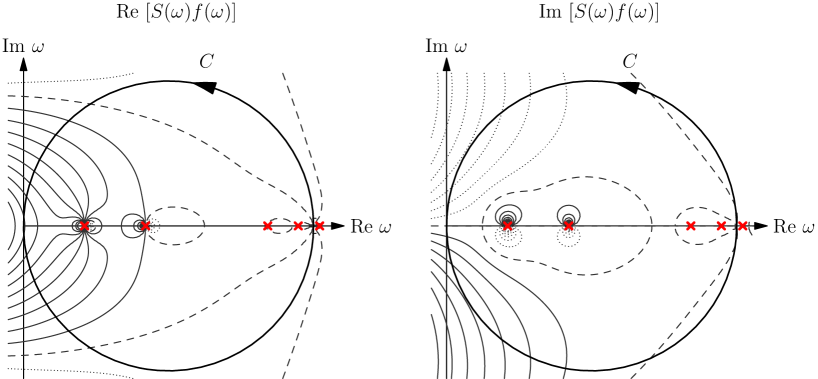
Figure 1: (Color online.) Schematic representation of the integration contour $C$ used to evaluate beta-decay rates. Only the poles of the strength function below the endpoint energy $\omega_{\text{max}}$ contribute to the decay rate.

The analog of Eq. (32) for first-forbidden beta decay is lengthy and presented in the Appendix B.

III Computational Method and Tests

As mentioned, our method begins with the use of the code hfbtho Stoitsov et al. (2005, 2013) to carry out an axially-deformed HFB calculation. In our tests 16 harmonic oscillator shells are enough to allow the low-energy strength functions to converge, and we adopt that number for all half-life calculations.

Our contour integration requires a reasonably accurate polynomial approximation to the Fermi integrals in Eq. (48). Figure 2 illustrates the quality of our fit to the allowed-decay Fermi integral. In practice, a 10th-order polynomial of the form (31) is more than sufficient. Another requirement is that the integrands are smooth enough to allow numerical quadrature. Figure 3 demonstrates that that is the case, displaying a typical integrand as a function of the curve parameter $t$ in Eq. (33). The integrand is indeed smooth enough to treat with conventional quadrature; we use the compound Simpson’s $3/8$ rule.

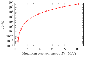
Figure 2: (Color online.) A 14th-order polynomial approximation to the phase space integral $f(E_{0})$ (Eq. (24)) for the beta decay of ¹⁴⁸Ba. The solid line is calculated with the exact Fermi function $F_{0}$ (Eq. (25)) and the points correspond to the polynomial approximation (31).

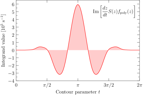
Figure 3: (Color online.) The imaginary part of the integrand in Eq. (32) that determines the $K=0$ allowed decay rate of ¹⁴²Ba, with SkO and the tensor interaction. The integrand behaves well enough to allow simple quadrature. The origin in the complex plane corresponds to $t=\pi$ (see text).

To test the pnfam solver itself, we compare in Fig. 4 the pnFAM Gamow-Teller transition strength function in the deformed isotope ²²Ne with that produced by the traditional matrix-QRPA code used in Ref. Mustonen and Engel (2013). The matrix code uses the Vanderbilt HFB solver Terán et al. (2003) as its starting point. The slight differences between the two strength functions are due to similarly slight differences in the HFB solutions, which in turn stem from different single-particle bases and truncation schemes.

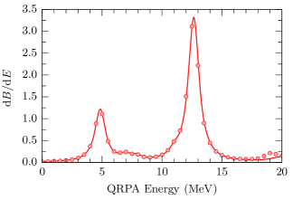
Figure 4: (Color online.) Comparison of the pnFAM Gamow-Teller strength function (points) in the deformed nucleus ²²Ne with the same function from the matrix QRPA (lines), smeared with a Lorentzian. We use the Skyrme functional SkM* without including $\mathbb{J}^{2}$ terms or pairing in the QRPA.

Finally, we turn to our prescription for the nuclear moment of inertia. The approximation in Eq. 22 appears to yield systematically higher values than does experiment, indicating that almost none of the nuclei we examine below are as rigid as the straightforward extension of the Beliaev formula predicts. (We can implement a better approximation that takes into account RPA correlations — the Thouless-Valatin prescription Thouless and Valatin (1962) — once a like-particle FAM for general $K$ exists.) To assess the sensitivity of the Gamow-Teller half-life to the rotational energy correction, we use the SkO functional detailed in the next section to calculate half-lives in a few test nuclei (Fig. 5). Although the strong dependence of the phase-space integral on the energy released in the decay can make a correction of the order of ten percent to the half-life, that error is still at most comparable to the error in the calculated $Q$ value. The accuracy of the generalized Beliaev moment of inertia is therefore good enough for use with present-day energy functionals.

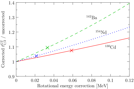
Figure 5: (Color online.) Partial Gamow-Teller half-lives in several nuclei as a function of rotational energy correction, normalized to the uncorrected values. The marker on each curve indicates the correction obtained from Eq. (22).

IV Results and Discussion

Recent work Bai et al. (2009a, b, 2011); Minato and Bai (2013) on semi-magic nuclei in the spherical QRPA indicates that tensor terms in Skyrme EDFs have significant effects on beta-decay rates. Here we explore the issue in open shell nuclei, both spherical and deformed. We choose a set of isotopes for which both beta-decay rates and the allowed contribution to those rates have been measured. To make contact with Ref. Minato and Bai (2013) we use the same underlying SkO functional, with the same additional tensor piece (i.e. the interaction parameters $t_{e}=184.567\textrm{ MeV fm}^{5}$, $t_{o}=-108.567\textrm{ MeV fm}^{5}$, in the notation of Ref. Perlińska et al. (2004)). We also adopt the Ref. Minato and Bai (2013) procedure of breaking self-consistency by omitting the central $J^{2}$ terms from the HFB calculation while including them in the QRPA. Unlike Ref. Minato and Bai (2013), however, we include the rotational energy correction and we approximate the ground-state energy by the sum of the lowest proton and neutron quasiparticle energies. These differences in procedure have small effects on the $Q$ value and half-life (via the phase space available to emitted leptons). The last difference with Ref. Minato and Bai (2013): we use the quenched value $g_{A}=1.0$ rather than 1.27 for the axial-vector coupling constant.

We fit the constants in the isovector pairing interaction Eq. (6) to a three-point interpolation of measured separation energies. The SkO functional with this pairing interaction reproduces $Q$ values well, both with and without tensor terms.

Fig. 6 shows the ratios of computed and experimental partial Gamow-Teller half-lives for our set of nuclei. The tensor interaction systematically reduces the half-lives, as in the magic and semi-magic nuclei examined by Ref. Minato and Bai (2013). In our spherical nuclei, with or without open shells, the agreement with experiment improves dramatically. In the deformed isotopes, however, the half-lives with SkO tend to be quite low even without the tensor terms, which actually make the half-lives too short. The situation is thus more complicated than it seems when restricted to spherical systems.

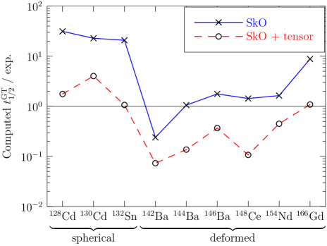
Figure 6: (Color online.) The ratio of computed and experimental partial Gamow-Teller half-lives. Two functionals are used: the bare SkO functional and the SkO functional with an added tensor piece. Isoscalar pairing is absent here.

Figure 7 shows the effects of the tensor interaction in more detail, in four isotopes. The new terms pull Gamow-Teller strength down in energy in each case, and smear the resonances. The movement of strength to lower energies explains the decrease in half-life; the lower-energy strength means more phase space for leptons and an increased rate.

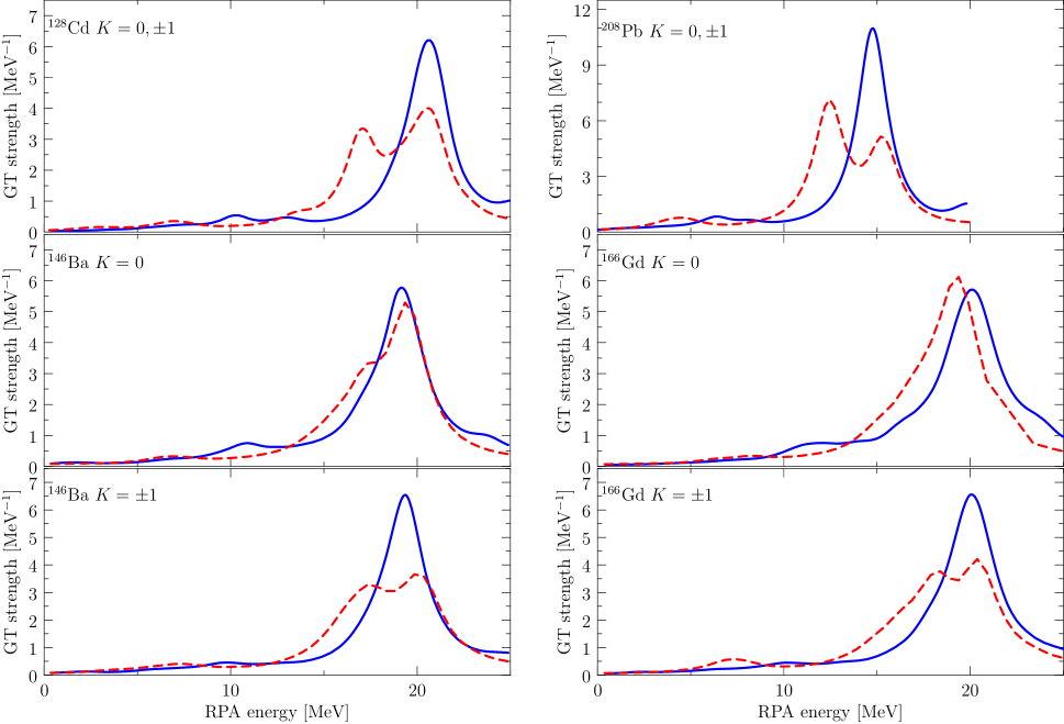
Figure 7: (Color online.) Gamow-Teller strength functions in several isotopes. The solid (blue) lines represent the strength without tensor terms and the dashed (red) lines the strength with those terms.

How many of the features in Figs. 6 and 7 are due to the violation of self-consistency between the HFB and QRPA calculations? How many are due to the limited set of nuclei that we examine? To the restriction to allowed decay? To the simple addition of a tensor interaction without any attempt to refit data? We can’t address these questions fully here, but can make a start. We now investigate a slightly larger set of nuclei (that overlaps our original set) with a fully self-consistent calculation that includes first-forbidden contributions to the rate. We choose as a starting point the functional SkO^′ Reinhard et al. (1999), which reproduces experimental $Q$ values as well as SkO and does a good job on beta-decay rates in semi-magic isotopes Engel et al. (1999). We adjust the time-odd part of the functional, setting $C^{\Delta s}_{1}=0$ to avoid instability (observed, e.g., in Schunck et al. (2010)) and $C^{s}_{1}=159\textrm{ MeV fm}^{3}$ to reproduce the Gamow-Teller resonance energy in ²⁰⁸Pb. We leave the other coupling constants untouched. When we include the tensor interaction we use the values implied by the Skyrme $t$ and $x$ parameters; the relations between these parameters and the $C$’s are given, e.g., in Ref. Perlińska et al. (2004). All this is the same prescription for the time-odd terms that was found practical (without tensor terms) in Ref. Bender et al. (2002).

Fig. 8 shows some of the results. Without the tensor interaction it is possible to roughly reproduce the half-lives through an appropriate strength for the isoscalar pairing interaction in Eq. 6 (about 60% of isovector interaction strength); in the analysis leading to Figs. 6 and 7 we did not include isoscalar pairing, which has been the most convenient remedy for many of the QRPA’s deficiencies. Ref. Minato and Bai (2013) suggests that the tensor interaction can obviate strong isoscalar pairing. To begin to test this idea, we add the same tensor terms we used with the SkO functional. There is no particular justification for this choice other than its successes with SkO and the lack of any work on tensor interactions in conjunction with SkO^′. Yet, as Figure 8 shows, these tensor terms lower the half-lives in very much the same way as isoscalar pairing.

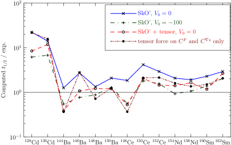
Figure 8: (Color online.) Ratio of calculated to experimental half-lives with the functional SkO^′and first-forbidden contributions included. The bare SkO^′ half-lives (solid blue line) are systematically longer than experiment and can be reduced by introducing either isoscalar pairing (dashed green line), a full tensor interaction (dashed red line), or only the time-odd components associated with such an interaction (dotted line).

As mentioned above, however, the simple addition of a tensor interaction spoils the functional’s ability to reproduce data. We have compensated for the problem in the time-odd channel by readjusting $C^{s}_{1}$, but have done nothing to repair the time-even channel, the original parameters of which were obtained through careful fits to energies, radii, etc. We therefore look at what happens when we leave the time-even part of SkO^′ alone, adding tensor terms to the time-odd part only. To make the changes truly minimal, we allow the tensor interaction to alter only the two time-odd coupling constants $C^{F}_{1}$ and $C^{\nabla s}_{1}$ that receive no contribution from any other piece of a typical density-dependent interaction. We again set $C^{\Delta s}=0$, and refit $C^{s}_{1}$ (now to 181 $\textrm{MeV fm}^{3}$) to reproduce the ²⁰⁸Pb resonance. Fig. 8 shows that even these modifications, which (again) do not alter other predictions, mimic much of the reduction in half-lives produced by isoscalar pairing.

These results suggest that the time-odd piece of the functional is much richer than previously suspected. The time is ripe for a much more careful analysis of all these terms. Our pnfam will allow data from charge-exchange reactions in deformed nuclei to be included in fits. A like-particle version would increase the range of usable data further. Together with modern optimization techniques, the efficient calculation of linear response should make for a vast improvement in our ability to describe beta decay and predict it in important $r$-process isotopes where measurement is not possible.

V Conclusions

We have adapted the finite amplitude method for the computation of beta-decay strength functions and rates in axially-deformed even-even nuclei with modern Skyrme-like energy-density functionals. While formally equivalent to the traditional matrix QRPA, the FAM is far more robust and just as useful as long as the full set of QRPA energies and transition-matrix elements is not needed.

To demonstrate the pnFAM’s power, we have taken a first look at the effect of Skyrme’s tensor terms on allowed and first-forbidden beta decay in open-shell isotopes. We find that the tensor interaction lowers half-lives in deformed nuclei much like it does in the spherical nuclei studied in Ref. Minato and Bai (2013). Working with the functional SkO^′, we are able to roughly reproduce measured rates in a range of nuclei without strong isoscalar pairing and without spoiling the predictions of the functional in even-even systems. It is clearly time to explore time-odd functionals systematically, and we intend to do so soon. Finally, beta decay is only one possible application of the pnFAM. Neutrino scattering, hadronic charge exchange, and double-beta decay are three others that come quickly to mind.

Appendix A Moment of Inertia

The Beliaev formula Beliaev (1961) for the moment of inertia in the BCS approximation is easy to extend to the HFB approximation. Writing the wave function of the rotating state to the first order in the rotational speed $\omega$

$$|\Psi\rangle=|\textrm{HFB}\rangle+\omega\sum_{\alpha<\beta}\frac{\langle\textrm{HFB}|a_{\beta}a_{\alpha}J_{x}|\textrm{HFB}\rangle}{E_{\alpha}+E_{\beta}}a^{\dagger}_{\alpha}a^{\dagger}_{\beta}|\textrm{HFB}\rangle\,,$$ (35)

yields for the moment of inertia

$$\mathcal{I}=\frac{1}{\omega}\langle\Psi|J_{x}|\Psi\rangle=\sum_{\alpha\beta}\frac{|\langle\textrm{HFB}|a_{\beta}a_{\alpha}J_{x}|\textrm{HFB}\rangle|^{2}}{E_{\alpha}+E_{\beta}}\,.$$ (36)

After applying this transformation to the operator $J_{x}$ and carrying out the contractions, we obtain the expression

$$\mathcal{I}=\sum_{\alpha\beta}\frac{|(U^{\dagger}J_{x}V^{*}-V^{\dagger}J_{x}U^{*})_{\alpha\beta}|^{2}}{E_{\alpha}+E_{\beta}}\,.$$ (37)

The Beliaev formula Beliaev (1961)

$$\mathcal{I}_{\textrm{Beliaev}}=2\sum_{k<k^{\prime}}\frac{|\langle k|J_{x}|k^{\prime}\rangle|^{2}}{E_{k}+E_{k^{\prime}}}(u_{k}v_{k^{\prime}}-v_{k}u_{k^{\prime}})^{2}$$ (38)

applies in the special case that the quasiparticle transformation is diagonal.

Appendix B First-forbidden Beta Decay

When forbidden operators contribute non-negligibly to beta decay, the transition strength $B_{i}$ in (23) must be replaced by a more general integrated shape function

$$\overline{C}_{J^{\pi}}=\frac{1}{f(E_{0})}\int_{1}^{W_{0}}\mathrm{d}W\,C_{J^{\pi}}(W)F_{0}L_{0}pW\left(W_{0}-W\right)^{2}.$$ (39)

Six different multipole operators contribute to non-unique first-forbidden decay:

$$\hat{\mathcal{O}}_{ps0}=\frac{\hbar c}{2M_{n}c^{2}}\bm{\sigma}\cdot\bm{\nabla}\,\tau_{-},$$ (40a)

$$\hat{\mathcal{O}}_{p}(K)=\frac{\hbar c\,\Theta_{K}}{2M_{n}c^{2}}\nabla_{K}\,\tau_{-},$$ (40b)

$$\hat{\mathcal{O}}_{r}(K)=\frac{\sqrt{3}\,\Theta_{K}}{R\lambdabar_{e}}\sqrt{\frac{4\pi}{3}}\,rY_{1K}(\hat{\mathbf{r}})\,\tau_{-},$$ (40c)

and

$$\hat{\mathcal{O}}_{rsL}(K)=\frac{(-1)^{L}\,\Theta(K)}{R\lambdabar_{e}}\sqrt{4\pi}\,r[\mathbf{Y}_{1}\bm{\sigma}]_{LK}\,\tau_{-},$$ (40d)

where $L=0,1,2$. Here $M_{n}=939.0$ MeV$/c^{2}$ is the nucleon mass, and $\lambdabar_{e}=\hbar c/(m_{e}c^{2})=386.159268$ fm is the (reduced) electron Compton wavelength. All operators and resulting quantities are normalized to the electron mass so that the quantity $\overline{C}_{J^{\pi}}$ in Eq. (39) is dimensionless Behrens and Bühring (1982). The factors $\Theta_{K}$ arise from the transformation from intrinsic to laboratory reference frames Bohr and Mottelson (1998):

$$\langle LK|\hat{\mathcal{O}}_{LK}|00\rangle=\Theta_{K}\langle K|\hat{\mathcal{O}}_{LK}|0\rangle,$$ (41)

where

$$\Theta_{K}=\begin{cases}1,&K=0\\ \sqrt{2},&K>0\end{cases}.$$ (42)

The shape factors for the non-unique forbidden decay are worked out e.g. in Ref. Suhonen (1993). Expressing the squared matrix elements and the interference terms in terms of residues and replacing the kinematic parts of integrands by polynomial expressions that closely approximate them along a portion of the real axis (see main text) one can write first-forbidden shape functions in the form

$$\overline{C}_{J^{\pi}}\approx\frac{1}{2\pi i}\sum_{i}\oint_{C}\mathrm{d}\omega\,P_{i}(\omega)R_{i}(J^{\pi};\omega)\,,$$ (43)

where the $R_{i}$ are linear combinations of functions $S(F;\omega)$ and $\chi(F,G;\omega)$ is defined in Eqs. (16) and (20). For $J^{\pi}=0^{-}$ we have

$$R_{1}(0^{-},\omega)=-\frac{2}{3}g_{A}^{2}\big{(}X_{+}S(\hat{\mathcal{O}}_{rs0};\omega)+\chi(\hat{\mathcal{O}}_{rs0},\hat{\mathcal{O}}_{ps0};\omega)\big{)}$$ (44a)

and

$$\begin{split}R_{2}(0^{-}&,\omega)=g_{A}^{2}\Bigg{[}\left(X_{+}^{2}+\frac{1}{9}\right)S(\hat{\mathcal{O}}_{rs0};\omega)\\ &+S(\hat{\mathcal{O}}_{ps0};\omega)+2X_{+}\chi(\hat{\mathcal{O}}_{rs0},\hat{\mathcal{O}}_{ps0};\omega)\Bigg{]}\,,\end{split}$$ (44b)

for $J^{\pi}=1^{-}$ we have

$$\begin{split}R_{1}(1^{-},\omega)=&-\frac{2}{9}\Big{[}X_{+}S(\hat{\mathcal{O}}_{r};\omega)-2g_{A}^{2}X_{-}S(\hat{\mathcal{O}}_{rs1};\omega)-g_{A}\sqrt{2}(X_{+}-X_{-})\chi(\hat{\mathcal{O}}_{r},\hat{\mathcal{O}}_{rs1};\omega)\\ &-\sqrt{3}\chi(\hat{\mathcal{O}}_{p},\hat{\mathcal{O}}_{r};\omega)+g_{A}\sqrt{6}\chi(\hat{\mathcal{O}}_{p},\hat{\mathcal{O}}_{rs1};\omega)\Big{]},\end{split}$$ (45a)

$$\begin{split}R_{2}(1^{-},\omega)=&S(\hat{\mathcal{O}}_{p};\omega)+\frac{1}{3}X_{+}^{2}S(\hat{\mathcal{O}}_{r};\omega)+\frac{2}{3}g_{A}^{2}X_{-}^{2}S(\hat{\mathcal{O}}_{rs1};\omega)-\frac{8}{27}\big{(}g_{A}^{2}S(\hat{\mathcal{O}}_{rs1};\omega)-\frac{g_{A}}{\sqrt{2}}\chi(\hat{\mathcal{O}}_{r},\hat{\mathcal{O}}_{rs1};\omega)\big{)}\gamma_{1}\\ &+\frac{1}{27}\big{(}S(\hat{\mathcal{O}}_{r};\omega)+2g_{A}^{2}S(\hat{\mathcal{O}}_{rs1};\omega)-2\sqrt{2}g_{A}\chi(\hat{\mathcal{O}}_{r},\hat{\mathcal{O}}_{rs1};\omega)\big{)}\\ &+\sqrt{\frac{2}{3}}\Big{(}-2g_{A}X_{-}\chi(\hat{\mathcal{O}}_{p},\hat{\mathcal{O}}_{rs1};\omega)-\sqrt{2}X_{+}\chi(\hat{\mathcal{O}}_{p},\hat{\mathcal{O}}_{r};\omega)+\frac{2}{\sqrt{3}}g_{A}X_{-}X_{+}\chi(\hat{\mathcal{O}}_{r},\hat{\mathcal{O}}_{rs1};\omega)\Big{)}\,,\end{split}$$ (45b)

$$\begin{split}R_{3}&(1^{-},\omega)=\frac{4}{3}\Big{[}-\frac{\sqrt{2}}{3}g_{A}X_{+}\chi(\hat{\mathcal{O}}_{r},\hat{\mathcal{O}}_{rs1};\omega)-\frac{2}{3}g_{A}^{2}X_{-}S(\hat{\mathcal{O}}_{rs1};\omega)+\sqrt{\frac{2}{3}}g_{A}\chi(\hat{\mathcal{O}}_{p},\hat{\mathcal{O}}_{rs1};\omega)\Big{]},\end{split}$$ (45c)

$$R_{4}(1^{-},\omega)=\frac{8}{27}g_{A}^{2}S(\hat{\mathcal{O}}_{rs1};\omega)\,,$$ (45d)

$$\begin{split}R_{5}(1^{-},\omega)&=\frac{1}{27}\Big{[}2S(\hat{\mathcal{O}}_{r};\omega)+g_{A}^{2}S(\hat{\mathcal{O}}_{rs1};\omega)\\ &-2\sqrt{2}g_{A}\chi(\hat{\mathcal{O}}_{r},\hat{\mathcal{O}}_{rs1};\omega)\Big{]},\end{split}$$ (45e)

$$\begin{split}R_{6}(1^{-},\omega)&=\frac{1}{27}\Big{[}2S(\hat{\mathcal{O}}_{r};\omega)+g_{A}^{2}S(\hat{\mathcal{O}}_{rs1};\omega)\\ &+2\sqrt{2}g_{A}\chi(\hat{\mathcal{O}}_{r},\hat{\mathcal{O}}_{rs1};\omega)\Big{]}\,,\end{split}$$ (45f)

and finally, for $J^{\pi}=2^{-}$ have

$$R_{5}(2^{-},\omega)=R_{6}(2^{-},\omega)=\frac{1}{9}g_{A}^{2}S(\hat{\mathcal{O}}_{rs2};\omega)\,.$$ (46)

We have used the shorthand

$$X_{\pm}=\left(\frac{W_{0}}{3}\pm\frac{\alpha Z}{2R}\right)\,,$$ (47)

where $\alpha$ is the fine-structure constant and $R$ is the nuclear radius. The polynomials $P_{k}(\omega)$ are fitted to the various integrated kinematical factors so that $P_{i}(\omega)\approx G_{i}((\omega_{\text{max}}-\omega)/(m_{e}c^{2})+1)$, with

$$G_{i}(W_{0})=\int_{1}^{W_{0}}\mathrm{d}W\,g_{i}F_{0}L_{0}p(W_{0}-W)^{2}\,$$ (48)

in the interval $\omega\in[0,\omega_{\text{max}}]$ (within our contour). Here

$$\begin{split}g_{1}&=\gamma_{1},\,g_{2}=W,\,g_{3}=W^{2}\,,\\ g_{4}&=W^{3},\,g_{5}=W(W_{0}-W)^{2}\,,\textrm{ and}\\ g_{6}&=\lambda_{2}W(W^{2}-1)\,,\end{split}$$ (49)

where the function $\lambda_{k}$ is

$$\lambda_{k}=\frac{(k+\gamma_{k})F_{k-1}}{k(1+\gamma_{1})F_{0}}\,.$$ (50)

The polynomial $P_{2}$ above is the same one that enters the computation of allowed decay. (We called it $f_{\textrm{poly}}$ in the main text.)

References

- Hayes et al. (2013) A. C. Hayes, J. L. Friar, G. T. Garvey, and G. Jonkmans, ArXiv:nucl-th/1309.4146 (2013).
- Mustonen and Engel (2013) M. T. Mustonen and J. Engel, Phys. Rev. C 87, 064302 (2013).
- Terasaki and Engel (2011) J. Terasaki and J. Engel, Phys. Rev. C 84, 014332 (2011).
- Nakatsukasa et al. (2007) T. Nakatsukasa, T. Inakura, and K. Yabana, Phys. Rev. C 76, 024318 (2007).
- Inakura et al. (2009) T. Inakura, T. Nakatsukasa, and K. Yabana, Phys. Rev. C 80, 044301 (2009).
- Avogadro and Nakatsukasa (2011) P. Avogadro and T. Nakatsukasa, Phys. Rev. C 84, 014314 (2011).
- Stoitsov et al. (2011) M. Stoitsov, M. Kortelainen, T. Nakatsukasa, C. Losa, and W. Nazarewicz, Phys. Rev. C 84, 041305(R) (2011).
- Minato and Bai (2013) F. Minato and C. L. Bai, Phys. Rev. Lett. 110, 122501 (2013).
- Bender et al. (2002) M. Bender, J. Dobaczewski, J. Engel, and W. Nazarewicz, Phys. Rev. C 65, 054322 (2002).
- Perlińska et al. (2004) E. Perlińska, S. G. Rohoziński, J. Dobaczewski, and W. Nazarewicz, Phys. Rev. C 69, 014316 (2004).
- Stoitsov et al. (2005) M. V. Stoitsov, J. Dobaczewski, W. Nazarewicz, and R. P, Comp. Phys. Comm. 167, 43 (2005).
- Stoitsov et al. (2013) M. V. Stoitsov, N. Schunck, M. Kortelainen, N. Michel, H. Nam, E. Olsen, J. Sarich, and S. Wild, Comp. Phys. Comm. 184, 1592 (2013).
- Schunck et al. (2010) N. Schunck, J. Dobaczewski, J. McDonnell, J. Moré, W. Nazarewicz, J. Sarich, and M. V. Stoitsov, Phys. Rev. C 81, 024316 (2010).
- Kortelainen et al. (2010) M. Kortelainen, T. Lesinski, J. Moré, W. Nazarewicz, J. Sarich, N. Schunck, M. V. Stoitsov, and S. Wild, Phys. Rev. C 82, 024313 (2010).
- Kortelainen et al. (2012) M. Kortelainen, J. McDonnell, W. Nazarewicz, P.-G. Reinhard, J. Sarich, N. Schunck, M. V. Stoitsov, and S. M. Wild, Phys. Rev. C 85, 024304 (2012).
- Kortelainen et al. (2013) M. Kortelainen, J. McDonnell, W. Nazarewicz, E. Olsen, P. G. Reinhard, J. Sarich, N. Schunck, S. M. Wild, D. Davesne, J. Erler, and A. Pastore, “Nuclear energy density optimization: Shell structure,” (2013), arXiv:1312.1746 .
- Klüpfel et al. (2009) P. Klüpfel, P.-G. Reinhard, T. J. Bürvenich, and J. A. Maruhn, Phys. Rev. C 79, 034310 (2009).
- Roca-Maza et al. (2012) X. Roca-Maza, G. Colò, and H. Sagawa, Phys. Rev. C 86, 031306 (2012).
- Lesinski et al. (2007) T. Lesinski, M. Bender, K. Bennaceur, T. Duguet, and J. Meyer, Phys. Rev. C 76, 014312 (2007).
- Bender et al. (2009) M. Bender, K. Bennaceur, T. Duguet, P. H. Heenen, T. Lesinski, and J. Meyer, Phys. Rev. C 80, 064302 (2009).
- Ring and Schuck (2004) P. Ring and P. Schuck, The Nuclear Many-Body Problem, 3rd ed. (Springer, 2004).
- Behrens and Bühring (1982) H. Behrens and W. Bühring, Electron Radial Wave Functions and Nuclear Beta-decay (International Series of Monographs on Physics) (Oxford University Press, USA, 1982).
- Schopper (1966) H. F. Schopper, Weak Interactions and the Nuclear Beta Decay (North-Holland Publishing Co., 1966).
- Suhonen (1993) J. Suhonen, Nucl. Phys. A 563, 205 (1993).
- Hardy and Towner (2005) J. C. Hardy and I. S. Towner, Phys. Rev. C 71, 055501 (2005).
- Primakoff and Rosen (1959) H. Primakoff and S. P. Rosen, Rep. Prog. Phys. 22, 121 (1959).
- Engel et al. (1999) J. Engel, M. Bender, J. Dobaczewski, W. Nazarewicz, and R. Surman, Phys. Rev. C 60, 014302 (1999).
- Terán et al. (2003) E. Terán, V. E. Oberacker, and A. S. Umar, Phys. Rev. C 67, 064314 (2003).
- Thouless and Valatin (1962) D. J. Thouless and J. G. Valatin, Nucl. Phys. 31, 211 (1962).
- Bai et al. (2009a) C. L. Bai, H. Q. Zhang, X. Z. Zhang, F. R. Xu, H. Sagawa, and G. Colò, Phys. Rev. C 79, 041301 (2009a).
- Bai et al. (2009b) C. L. Bai, H. Sagawa, H. Q. Zhang, X. Z. Zhang, G. Colò, and F. R. Xu, Phys. Lett. B 675, 28 (2009b).
- Bai et al. (2011) C. L. Bai, H. Q. Zhang, H. Sagawa, X. Z. Zhang, G. Colò, and F. R. Xu, Phys. Rev. C 83, 054316 (2011).
- Reinhard et al. (1999) P. G. Reinhard, D. J. Dean, W. Nazarewicz, J. Dobaczewski, J. A. Maruhn, and M. R. Strayer, Phys. Rev. C 60, 014316 (1999).
- Beliaev (1961) S. T. Beliaev, Nucl. Phys. 24, 322 (1961).
- Bohr and Mottelson (1998) A. Bohr and B. R. Mottelson, Nuclear Structure, Vol. 2 (World Scientific Pub Co Inc, 1998).