Retrieval in Long Surveillance Videos using User Described Motion & Object Attributes

Abstract

We present a content-based retrieval method for long surveillance videos both for wide-area (Airborne) as well as near-field imagery (CCTV). Our goal is to retrieve video segments, with a focus on detecting objects moving on routes, that match user-defined events of interest. The sheer size and remote locations where surveillance videos are acquired, necessitates highly compressed representations that are also meaningful for supporting user-defined queries. To address these challenges we archive long-surveillance video through lightweight processing based on low-level local spatio-temporal extraction of motion and object features. These are then hashed into an inverted index using locality-sensitive hashing (LSH). This local approach allows for query flexibility as well as leads to significant gains in compression. Our second task is to extract partial matches to the user-created query and assembles them into full matches using Dynamic Programming (DP). DP exploits causality to assemble the indexed low level features into a video segment which matches the query route. We examine CCTV and Airborne footage, whose low contrast makes motion extraction more difficult. We generate robust motion estimates for Airborne data using a tracklets generation algorithm while we use Horn and Schunck approach to generate motion estimates for CCTV. Our approach handles long routes, low contrasts and occlusion. We derive bounds on the rate of false positives and demonstrate the effectiveness of the approach for counting, motion pattern recognition and abandoned object applications.

I Introduction

Video surveillance camera networks are increasingly ubiquitous, generating thousands of hours of archived video every day. This data is rarely processed in real-time and primarily used for scene investigation purposes to gather evidence after events take place. In military applications UAVs produce terabytes of wide area imagery in real-time at remote/hostile locations. Both of these cases necessitate maintaining highly compressed searchable representations that are local to the user but yet sufficiently informative and flexible to handle a wide range of queries. While compression is in general lossy from the perspective of video reconstruction it is actually desirable from the perspective of search since it not only reduces the search space but it also leverages the fact that for a specific query most data is irrelevant and pre-processing procedures such as video summarization is often unnecessary and inefficient. Consequently, we need techniques that are memory and run-time efficient to scale with large data sets, and be able to retrieve video segments matching user defined queries with robustness to common problems, such as low frame-rate, low contrast and occlusion.

Some of the main challenges of this problem are:

1.) Data lifetime: since video is constantly streamed, there is a perpetual renewal of video data. This calls for a model that can be updated incrementally as video data is made available. The model must also scale with the temporal mass of the video.

2.) Unpredictable queries: the nature of queries depends on the field of view of the camera, the scene itself and the type of events being observed. The system should support queries of different nature that can retrieve both recurrent events such as people entering a store and infrequent events such as abandoned objects and cars performing U-turns.

3.) Unpredictable event duration: events are unstructured. They start anytime, vary in length, and overlap with other events. The system is nonetheless expected to return complete events regardless of their duration and whether or not other events occur simultaneously.

4.) Clutter and occlusions: Tracking and tagging objects in urban videos is challenging due to occlusions and clutter; especially when real-time performance is required.

This paper presents a method for fast content-based retrieval adapted to characteristics of surveillance videos. Our technique is query-driven where the user draws routes manually. The algorithm then retrieves video segments containing objects that moved in the user supplied routes. Our technique consists of two steps: The first extracts low level features and hashes them into an inverted index using locality-sensitive hashing (LSH). The second stage extracts partials matches and assembles them into full matches using Dynamic Programming (DP).

We examine two types of data: (1) CCTV and (2) Airborne. Airborne footage contains aerial view images shot from a UAV. Their processing is more challenging than CCTV due to their lower frame rate and lower contrast (see Fig. 1 ). From this footage we are able to extract a number of low level features, described in Section IV. Here certain features such as optical flow information (extracted using Horn and Schunck technique [8]) are rendered highly noisy due to the Airborne low contrast. Hence for Airborne footage we first generate tracklets, using ideas from [20, 6], and then generate motion estimates from those tracklets. Our technique retrieves routes generated by different objects (such as cars and human), handles long routes, low-contrast, occlusion, and performs faster than current techniques.

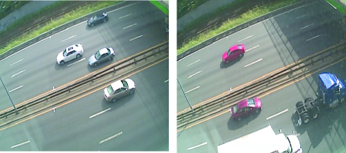
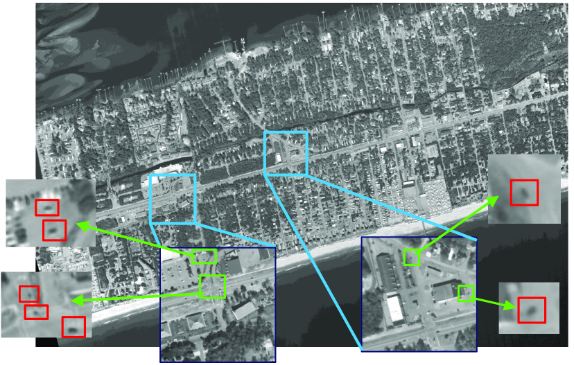
Figure 1: Top: Examples of CCTV footage. Bottom: Example of Airborne footage. Blue and green boxes show zoomed-in regions. Objects of interests (cars in this figure) usually have much lower contrast in Airborne footage (see red boxes) over CCTV footage. This makes processing Airborne footage more challenging than CCTV.

II Related Work

Most video papers devoted to summarization and search focus on broadcast videos such as music clips, sports games, movies, etc. These methods typically divide the video into “shots” [37, 28] by locating key frames corresponding to scene transitions. The search procedure exploits key frame content and matches either low-level descriptors [28] or higher-level semantic meta-tags to a given query [37].

Surveillance videos are fundamentally different than conventional videos. Not only do surveillance videos have no global motion induced by a moving camera, they often show unrelated or unimportant moving and static objects. For that reason, surveillance videos are difficult to decompose into “scenes” separated by key frames that one could summarize with some meta tags or a global mathematical model. Furthermore, surveillance videos generally have no closed-caption or audio track  [37].

For that reason, search in a surveillance video focuses on understanding and indexing the dynamic content of the video in a way that is compatible with arbitrary upcoming user-defined queries. Thus, most scene-understanding video analytic methods work on a two-stage procedure:

• Learn patterns of activities via a clustering/learning procedure

• Recognize new patterns of activity via a classification stage.

For the first stage many methods are based on the fact that activities in public areas often follow some basic rules (traffic lights, highways, building entries, etc). Therefore, during the learning stage these methods often quantize space and time into a number of states with transition probabilities. Common models are HMMs [21, 16, 15], Bayesian networks [10, 33], context free grammars [31], and other graphical models [25, 32]. During the classification stage these learned patterns are either used to recognize pre-defined patterns of activity [36, 13, 25, 23, 35] (useful for counting [30]) or to detect anomalies by flagging everything that deviates from what has been previously learned [22, 21, 15]. We also note that that some of these methods that account for global behavior understanding often rely on tracking [15, 21, 10] while those devoted to isolated action recognition rely significantly on low-level features [13, 23, 36].

Although these methods could probably be adapted to index the video and facilitate search, very few methods this problem explicitly [18]. An exception is a method based on topic modeling by Wang et al. [32]. Their method decomposes the video into clips in which the local motion is quantized into words. These words are than clustered into so-called topics such that each clip is modeled as a distribution over these topics. They consider queries that are mixtures of these topics. Consequently, their search algorithm fetches every clip containing all of the topics mentioned in the query. A similar approach can be found in [34, 11, 33, 16] But search techniques focused on global explanations operate at a competitive disadvantage: the preponderance of clutter (4th issue in the introduction) in surveillance video makes the training step of scene understanding prohibitively difficult. Second, since these techniques often focus on understanding recurrent activities, they are unsuited for retrieving infrequent events - this can be a problem, given that queries are unpredictable (2nd issue in the introduction), and some activities of interest may seldom occur. Finally, the training step in scene understanding can be prohibitively expensive (3rd issue in introduction) for large data lifetimes.

Other related methods have also been developed but often customized to specific applications. For instance, Stringa et al. [27] describe a system to recover abandoned objects, Lee et al. [17] create a user interface to retrieve basic events such as the presence of a person, Meesen et al. [19] present an object-based dissimilarity measure to recover objects based on low-level features, and Yang et al. [34] store human-body meta tags in a SQL table to humanoid shapes based on their skin color, body size, height, etc.

II-A Our Contributions

In this paper, we extract a full set of low-level features as we have no a priori knowledge of what query will be asked. This is different from search procedures relying on high level information such as tracking [14] and human shape detection [29]. Unlike scene understanding techniques, we have no training step; this would be incompatible with the data lifetimes and magnitude of the video corpus. Instead, we develop an approach based on exploiting temporal orders on simple features, which allows us to find arbitrary queries quickly while maintaining low false alarm rates. We demonstrate a substantial improvement over scene-understanding methods such as [33, 16] on a number of datasets in Section VII.

III Overview

To address the challenges of exploratory search, we utilize a two-step procedure that first reduces the problem to the relevant data, and then reasons intelligently over that data. This process is shown in Fig. 2. As data streams in, video is pre-processed to extract low-level features - activity, object size, color, persistence and motion. For CCTV footage, motion is estimated using Horn and Shunck approach  [8]. For Airborne footage, motion is estimated using tracklets. These low-level features are hashed into a fuzzy, light-weight lookup table by means of LSH [12]. LSH accounts for spatial variability and reduces the search space for a user query to the set of relevant partial (local) matches.

The second step is a search engine optimization which reasons over the partial matches to produce full matches; segments of video which fit the entire query pattern, as opposed to part of it. This optimization operates from the advantageous standpoint of having only to reason over the partial matches, which are the relevant subset of the video. In surveillance video, where a long time can pass without relevant action, this dramatically reduces the workload of the optimization algorithm.

We then present two solutions for finding full matches. The first is a greedy approach which flattens the query in time. The second, a novel dynamic programming (DP) approach, exploits the causal ordering of component actions that makeup a query. DP reasons over the set of partial matches and finds the best full match. We present two DP versions, one that uses optical-flow (for CCTV) and another that uses tracklets (for Airborne). We also show that as actions become more complex, the number of false positives in a surveillance environment goes to zero.

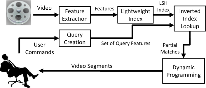
Figure 2: From streaming video, low level features for each document are computed and inserted into a fuzzy, lightweight index. A user inputs a query, and partial matches (features which are close to parts of the query) are inserted into a dynamic programming (DP) algorithm. The algorithm extracts the set of video segments which best matches the query.

IV Feature extraction

In this section we describe the process of low-level feature extraction. We first explain the data structure used in our technique, then discuss feature extraction for CCTV and Airborne footage.

IV-A Structure

For the purpose of feature extraction, a video is considered to be a spatio-temporal volume of size $H\times W\times F$ where $H\times W$ is the image size in pixels and $F$ the total number of frames in the video. The video is divided along the temporal axis into contiguous documents each containing $A$ frames. As shown in Fig.  3, each frame is divided into tiles of size $B\times B$. An atom is formed by grouping the same tile over $A$ frames. These values vary depending on the size of the video - for our videos, we chose B equal to 8 or 16 pixels, and A equal to 15 or 30 frames, depending on frame rate. As the video streams in, features are extracted from each frame. Whenever a document is created, each atom $n$ is assigned a set of features (see Sec. IV-B and Sec. IV-C) describing the dynamic content over that region.

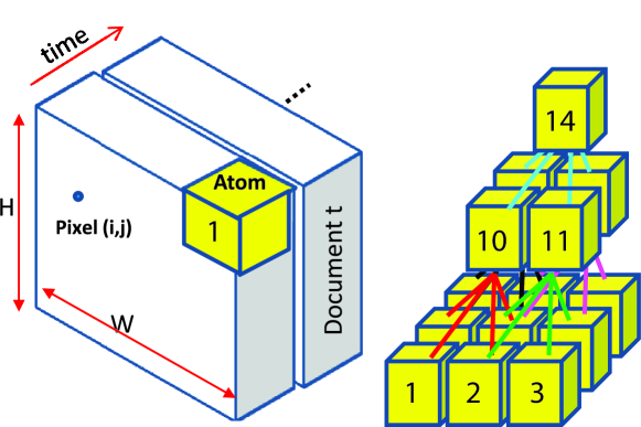
Figure 3: (Left) Given an $W\times H\times F$ video, documents are non-overlapping video clips each containing $A$ frames. Each of the frames are divided into tiles of size $B\times B$. Tiles form an atom when aggregated together over $A$ frames. (Right) Atoms are grouped into trees - every adjacent set of four atoms is aggregated into a parent, forming a set of partially overlapping trees.

We construct a pyramidal structure to robustify our algorithm to location and size variability in detected features. Each element of the pyramid has four children. Since trees overlap, a $k$-level trees contains $M=\sum_{l=1}^{k}l^{2}$ nodes as shown in Fig. 3. In this approach, a document containing $U\times V$ atoms will be assigned $(U-k+1)\times(V-k+1)$ partially overlapping trees to be indexed. For instance, in Figure 3, we draw a depth-3 tree which aggregates $3\times 3$ atoms. This tree contains $M=14$ nodes.

Each node of a tree is assigned a feature vector obtained by aggregating the feature vector of its children nodes. Let $n$ be a non-leaf node and $a,b,c,d$ its four children. The aggregation process can be formalized as

$$\vec{x}_{f}^{(n)}=\psi_{f}\left(\vec{x}_{f}^{(a)},\vec{x}_{f}^{(b)},\vec{x}_{f}^{(c)},\vec{x}_{f}^{(d)}\right),$$

where $\psi_{f}$ is an aggregation operator for the examined features. The resulting quantity is $\vec{x}_{f}^{(n)}$, a concatenation of all features. Sec. IV-B and Sec. IV-C present more details on the aggregation operator. Given that several features are extracted for each atom, aggregating a group of $k\times k$ atoms results in a set of feature trees $\left\{\operatorname{tree}_{f}\right\}$, one for each feature $f$. Given that a $k$-level tree contains $M$ nodes, each $\operatorname{tree}_{f}$ contains a list of $M$ feature instances, namely $\operatorname{tree}_{f}=\left\{\vec{x}_{f}^{(n)}\right\}$.

IV-B Feature Extraction for CCTV footage

As reported in the literature  [19, 27, 34], atom features can be of any kind such as color, object shape, object motion, tracks, etc. We chose to use local processing due to the computational efficiency which makes it better suited to the constant data renewal constraint and real-time feature extraction. Because our focus is surveillance video, we assume a stable camera. Feature extraction computes a single value for each atom, which is aggregated into feature trees. Our method uses the following five features:

(1) Activity $x_{a}$: Activity is detected using a basic background subtraction method  [7]. The initial background is estimated using a median of the first 500 frames. Then, the background is updated using the running average method. At the leaf level, $x_{a}$ contains the proportion of active pixels within the atom. Aggregation for non-leaf nodes in feature trees, $\psi_{a}$, is the mean of the four children.

(2) Blob Size $x_{s}$: Moving blobs are detected using connected components analysis of the binary activity mask obtained from background subtraction [7]. Blob size is the total number of active pixels covered by the connected component. The aggregation operator $\psi_{s}$ for non-leaf nodes in feature trees is the median of non-zero children. Whenever all four children have a zero size, the aggregation operator returns zero.

(3) Color $\vec{x}_{c}$: Color is obtained by computing the quantized histogram over every active pixel in the atom. RGB pixels are then converted to the HSL color space. Hue, saturation and luminance are quantized into 8, 4 and 4 bins respectively. The aggregation operator $\psi_{a}$ for non-leaf nodes in feature trees is the bin-wise sum of histograms. In order to keep relative track of proportions during aggregation, histograms are not normalized at this stage.

(4) Persistence $x_{p}$: Persistence is a detector for newly static objects. It is computed by accumulating the binary activity mask obtained from background subtraction over time. Objects that become idle for a long periods of time thus get a large persistence measure. The aggregation operator $\psi_{p}$ for non-leaf nodes in feature trees is the maximum of the four children.

(5) Motion $\vec{x}_{m}$: Motion vectors are extracted using Horn and Schunck optical flow method  [8]. Motion is quantized into 8 directions and an extra “idle” bin is used for flow vectors with low magnitude. $\vec{x}_{m}$ thus contains a 9-bin motion histogram. The aggregation operator $\psi_{m}$ for non-leaf nodes in feature trees is a bin-wise sum of histograms. In order to keep relative track of proportions during aggregation, histograms are not normalized at this stage.

As mentioned previously, these motion features are extracted while the video streams in. Whenever a document is created, its atoms are assigned $5$ descriptors, namely $\left\{x_{a},x_{s},\vec{x}_{c},x_{p},\vec{x}_{m}\right\}$. These descriptors are then assembled to form the $5$ feature trees $\left\{\operatorname{tree}_{a}\right\}$, $\left\{\operatorname{tree}_{s}\right\}$, $\left\{\operatorname{tree}_{c}\right\}$, $\left\{\operatorname{tree}_{p}\right\}$, $\left\{\operatorname{tree}_{m}\right\}$. These feature trees are the basis for the indexing scheme presented in section  V. After feature trees are indexed, all extracted feature content is discarded, ensuring a lightweight representation. It is worth noting that these features are intentionally simple. This speeds up feature extraction and indexing while being robust to small distortions due to the coarse nature of the features. While motion can be sensitive to poorly-compensated camera motion or zoom, and color can be sensitive to illumination changes, the other features have been shown relatively robust to these effects [7]. In addition, we leverage on the dynamic programming in section VI-B2 to limit false activity detection.

IV-C Feature Extraction for Airborne Footage

In order to be robust to issues of low contrast and low frame-rate in airborne data, we extract tracklets and then derive features from them. Our tracklet extraction process uses a Viterbi-style algorithm with ideas from Pitie et al. [20] and Baugh et al. [6]. At each frame, we generate a set of candidates to be tracked and update existing tracklets with these candidates based on distance in feature and position space.

We are supplied with Airborne footage stabilized with respect to the global camera motion. In order to identify moving objects (cars and people) we use frame differencing. Consecutive frames are used for cars, and frames spaced by 10 for slower-moving humans. We use a very small detection threshold to ensure all false negatives are eliminated. Cars are detected if a frame difference of more than $15$ gray-scale levels is observed. A smaller threshold of $10$ is used for humans detection as they have lower contrast. Some detection errors often occur around borders of trees and objects (see Fig. 4, red region). Other artifacts are caused due to local motions as the ones generated by the moving sea waves (see Fig.4, blue region). Such artifacts are removed through filtering by size. Here we first detect connected bodies and remove any body that contains more than $150$ pixels.

An example of candidate selection with artifacts removal is shown in Fig.4. Note that filtering by size eliminates the vast majority of false alarms. This is evident by examining the blue and red rectangles of Fig. 4 before and after filtering (third and fourth columns respectively). Quantitative results show that this filtering reduces false alarms by $72.3\%$ and $96.5\%$ for cars and humans respectively. This is taken as the average over processing $1000$ frames for each of Task 12 and 13 ( see table I ). It is worth noting that our algorithm only detects moving vehicles and humans. Stopped vehicles are dealt with by our dynamic programming algorithm which we introduce in Section VI-B2.

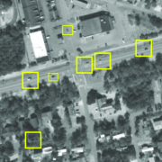
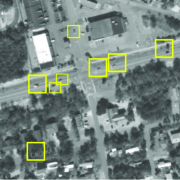
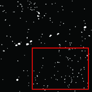
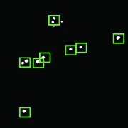
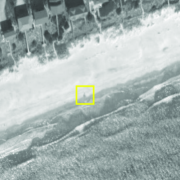
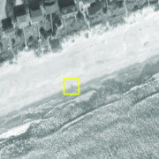
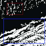
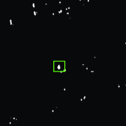
Figure 4: First row, from left: Two consecutive frames showing cars (shown in yellow) moving near a junction, (c) Frame subtraction and (d) result after applying morphological opening. The final result (d) is void of noisy data shown in red in (c). Second row, from left: Two frames showing a group of people (shown in yellow) walking near a beach, (g) detection after applying morphological opening and (h) detected candidates of size more than 150 pixels in green.

Given a set of detection candidates, our goal is to associate them over time for the purposes of computing tracklets. To do so, we set up and solve a Viterbi Trellis as described in [6]. Given a set of detection candidates in frame $n$ and $n+1$, we estimate the temporal matching cost of each detection pair as follows

$$\mathcal{C}_{l,m}=\Lambda_{1}\|p_{l}-p_{m}\|+\Lambda_{2}|z_{l}-z_{m}|$$

$$+\Lambda_{3}f_{3}(s_{l},s_{m})+\Lambda_{4}f_{4}(c_{l},c_{m})+\Lambda_{5}f_{5}(p_{l},p_{m}).$$ (1)

Here $l$ and $m$ denote the examined candidate of frame $n$ and $n+1$ respectively. $(p\;s\;z\;c)$ are the position, shape, size and color of each examined candidate. $\Lambda_{1}...\Lambda_{5}$ are tunable weights to emphasize the importance of each term. Position is defined as the geo-registered location, shape is the binary mask of the occupied pixels and size is the number of pixels in the examined mask. The purpose of the five elements of Eq. (1) is to ensure that the target: (1) has not moved too far between $n$ and $n+1$, (2) is roughly the same size, (3) the same shape, (4) the same color and (5) it is roughly where we expect it to be given its previous motion and location.

$s_{l}$ and $s_{m}$ are binary detection masks for the targets under examination, where $f_{3}(s_{l},s_{m})$ is the mean absolute error between both masks. Given the color measurements of the examined candidates $c_{l}$ and $c_{m}$, we fit a GMM for $c_{l}$ being $G(c_{l})$ [9]. We then estimate $f_{4}(c_{l},c_{m})$ as the error of generating $c_{m}$ from $G(c_{l})$ [9]. To calculate $f_{5}(p_{l},p_{m})$ we first estimate the expected location of $l$ in the next frame ($n+1$) given its current location in frame $n$. The expected location is estimated using a 3 frame window and a straight line, constant acceleration model. $f_{5}(p_{l},p_{m})$ is then taken as the absolute difference between the expected location of $l$ in $n+1$ and the actual location of $m$.

Given the matching costs for all possible $l$ and $m$ pairs, we approximate the two-dimensional assignment problem by greedy assignment for computational efficiency. That is we match the pairs with least matching cost first, remove them, match the next pair, remove them and keep doing so until all candidates in frame $n$ are matched with candidates in frame $n+1$. Note that this is a one-one assignment process hence no candidate in either frame $n$ or $n+1$ can have more than one match. This assignment, plus efficient computation of $f_{4}$, yield a simple tracking approach that can scale to large datasets.

Fig. 5 shows examples of tracklets generated by the technique discussed in this section. Here we show tracklets of cars (see left of Fig. 5) and for a group of people walking on the beach (see right of Fig. 5). Note that our tracklets generator assumes temporal consistency and hence it disregards false detections that are temporally inconsistent. This further removes detection artifacts. In closing, note that we do not need particularly good long-term tracks; we need tracks good enough for our retrieval problem.

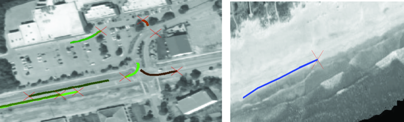
Figure 5: Examples of tracklets generated by the technique discussed in Sec. IV-C. Here tracks start with a red cross and their tails have different color. The example of the left shows tracklets generated for cars while the example on the right shows tracklet generated for a group of people walking on the beach.

V Indexing & Hashing

When a document is created, features are aggregated into $(U-k+1)\times(V-k+1)$ $k$-level trees. For CCTV data, each tree is made of $5$ feature trees, namely $\left\{\operatorname{tree}_{a}\right\},\left\{\operatorname{tree}_{s}\right\},\left\{\operatorname{tree}_{c}\right\},\left\{\operatorname{tree}_{p}\right\},\left\{\operatorname{tree}_{m}\right\}$. For Airborne data there is one feature tree, namely $\left\{\operatorname{tree}_{d}\right\}$. $\left\{\operatorname{tree}_{d}\right\}$ is a 1-level tree that stores the current-to-next frame displacements for all points of the generated tracks.

To index a given feature tree $\operatorname{tree}_{f}$ efficiently, our method uses an inverted index for content retrieval. Inverted index schemes, which map content to a location in a database, are popular in content-based retrieval because they allow extremely fast lookup in very large document databases. For video, the goal is to store the document number $t$ and the spatial position $(u,v)$ in the database based on the content of $\operatorname{tree}_{f}$. This is done with a mapping function which converts “$\operatorname{tree}_{f}$” to an entry in the database where $(t,u,v)$ is stored. Two trees with similar contents, therefore, should be mapped to proximate locations in the index; by retrieving all entries which are near a query tree, we can recover the locations in the video of all features trees that are similar. Note that for Airborne data, in addition to storing $(t,u,v)$ for each tree, we also store the track ID. This encourages results to be generated from as few tracks as possible and hence makes solution more robust to clutter.

This mapping and retrieval can be made for which update and lookup exhibit flat performance ($O(1)$ complexity). Because similar content at different times is mapped to the same bin, the time required to find the indices of matching trees does not scale with the length of the video. Obviously, the total retrieval time must scale linearly with the number of matching trees, but this means that the run-time of the retrieval process scales only with the amount of data which is relevant. In videos where the query represents an infrequently-performed action, this optimization yields an immense improvement in runtime.

Hashing: A hash-based inverted index uses a function to map content to an entry in the index. This is done with a hashing function $h$ such that $h:\operatorname{tree}_{f}\to j$, where $j$ is a hash table bucket number. In this paper, we use a locally-sensitive hashing (LSH) function [12]. LSH is a technique for approximation of nearest-neighbor search. In contrast to most hashing techniques, LSH attempts to cluster similar vectors $\vec{x}$ and $\vec{y}$ by maximizing the probability of collisions for descriptors within a certain distance of each other:

$$\vec{x}\approx\vec{y}\implies P\left\{h(\vec{x})=h(\vec{y})\right\}\gg 0.$$

If feature trees are close in Euclidean distance (the element-wise square of the distances between node values in the two trees is small), then the probability of them having the same hash code is high. Because our feature trees contain $M$ real-valued variables, LSH functions can be drawn from the p-stable family:

$$h_{\vec{a},b,r}(\operatorname{tree}_{f})=\left\lfloor\frac{\vec{a}\cdot\operatorname{tree}_{f}+b}{r}\right\rfloor,$$

where $\vec{a}$ is a $M$-dimensional vector with random components drawn from a stable distribution, $b$ is a random scalar drawn from a stable distribution and $r$ is an application-dependent parameter. Intuitively, $\vec{a}$ represents a random projection, an alignment offset $b$ and a radius $r$ controlling the probability of collision inside the radius.

Indices $I_{f}$ are built and searched independently for each feature. Thus, the database is made of five indices for the CCTV data and two indices for the Airborne data. Here there is one database index for each feature $f$. Each index $I_{f}$ is composed of a set of $n$ hash tables $\left\{T_{f,i}\right\},~{}\forall i=1,\ldots,n$. Each hash table is associated to its own hash function $H_{f,i}$ drawn from the p-stable family $h_{\vec{a},b,r}$. The parameter $r$ can be adjusted to relax or sharpen matches. In our implementation, $r$ is fixed for a given feature. The random parameters $\vec{a}$ and $b$ ensure projections from the different hash functions complement each other.

Given a feature tree $\operatorname{tree}_{f}$ at location $u,v$ with hash code $H_{f,i}(\operatorname{tree}_{f},u,v)=j$, $T_{f,i}[j]$ denotes the set of document numbers $\left\{t\right\}$ such that feature trees at $(t,u,v)$ have similar content. Lookup in the index $I_{f}$ consists of taking the union of document numbers returned by lookup in all tables $\left\{T_{f,i}\right\}$:

$$I(\operatorname{tree}_{f},u,v)=\displaystyle\cup_{i=1}^{n}T_{f,i}\left[H_{f,i}(\operatorname{tree}_{f}),u,v\right].$$

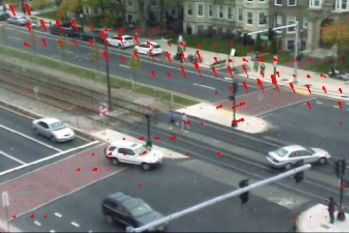
(a) (b)

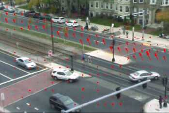
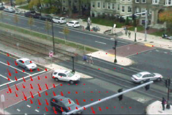
(c) (d)

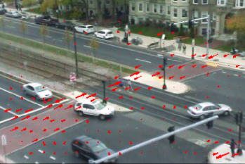
Figure 6: Contents of four buckets of a hash table for the motion feature. Arrows size is proportional to the number of hits at the specified location across the entire video. The hash buckets are associated to activity (a) side walk (b) upper side of the street (c) lower side of the street (d) crosswalk.

Fig.  6 illustrates several feature trees partitioned into groups, where trees in the same group have been given the same hashing key. For a given video, we plotted the content of four of the most occupied buckets for the motion feature $\operatorname{tree}_{m}$. As one can see, the trees associated to similar motion patterns in various parts of the scene have been coherently hashed into similar buckets.

Lightweight Storage: In contrast to approaches relying on a distance metric, such as K-nearest neighbor search, the hash-based index representation does not require storage of feature descriptors. $T_{f,i}$ contains only document numbers $\left\{t\right\}$, which are stored in $4$-byte variables. Our features, being local and primitive, are dependent on foreground content. As such, both our indexing times and storage scale linearly with the amount of foreground content in the video. This is a useful feature for surveillance video, which can have persistently inactive spaces or times throughout a video. For example, the size of the index for a 5 hour video with an activity rate of $2.5\%$ is only 150kb while the input color video requires almost 7Gb (compressed).

Building Lookup Table: As video streams in, the index for each feature is updated by a simple and fast procedure. After extraction of feature $f$ for document $t$ is completed, the extracted features are grouped into trees, as described in Sec. IV. Then, $I_{f}$ is updated with the mapping $\operatorname{tree}_{f}\to(t,u,v)$ for each tree position $(u,v)$ covering an area with significant activity. This is repeated for each feature $f$.

VI Search engine

We showed how to extract low-level features from a video sequence, bundle them into trees and index them for $O(1)$ content-based retrieval. Here we explain how to use feature index for high-level search.

VI-A Queries

In video search without exemplars, it is essential to provide a straightforward way for a user to input a query. For our , a query is defined as an ordered set of action components (for simple queries, a single component frequently suffices), each of which is a set of feature trees. To create a query, the user types in the number of action components, and is then presented with a GUI, shown in Figure 7 containing the first frame of the video to search for each of the action components. The user then selects the type of feature he wishes to search for, and draws the region of interest (ROI) that he wishes to find it in. These regions and the features (directions of motion, in this case) are shown in Fig.10 as green areas and red arrows, respectively.

As an example, to describe a u-turn, the user might describe three action components: one detecting motion approaching an intersection, one detecting motion turning around, and one detecting motion leaving the intersection. Likewise, a man hopping a subway might be represented by somebody approaching the subway, jumping up, and then continuing past the subway.

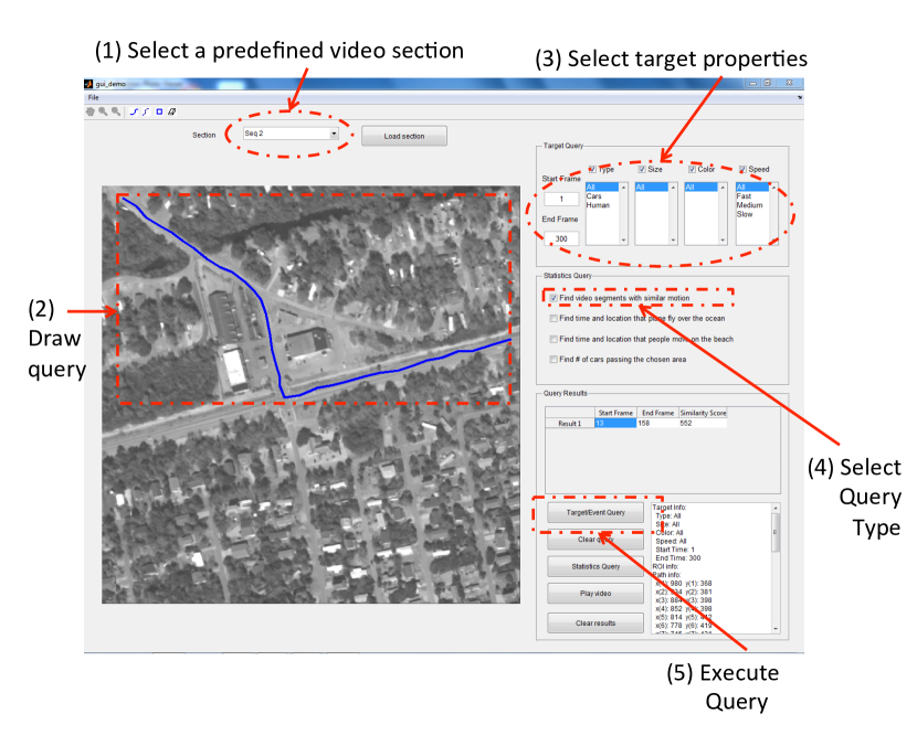
Figure 7: The query creation GUI provides a straightforward way to construct queries. The user draws each action component (shown in blue), and can additionally specify features.

Because our features (activity, size, color, persistence and motion) are semantically meaningful, this method of input is a relatively accessible way to define a query. After the features and the ROI are selected, a feature tree $tree_{f}$ is created to represent that action component. Note that this formulation provides the user with a way to produce a complex query vocabulary. A single component could describe a search for ”small red stationary blob” or ’large blob moving to the right”. While our claims to simplicity are theoretical, they are also supported by anecdotal evidence. People unfamiliar with the system are able to create their own queries in under a minute after a brief explanation of the tools.

After the action component has been input, the set of feature trees is extracted from it using the formulation in Section IV. These feature trees is used to query the inverted index of Section V to produce a set of documents and locations called partial matches $M(q)$. $M(q)$ is a list of spatio-temporal positions $(u,v,t)$ which contain similar trees to query $q$. In the case where the query contains multiple feature trees, the set of matching locations is the intersection of the matches for individual trees. Fig.10 presents 10 queries with their ROI.

VI-B Full matches

Search in a surveillance video requires more than partial matches. Activities in a video are inherently complex and show significant variability in time duration. For instance, a fast car taking a U-turn will span across fewer documents and generate different motion features than a slow moving car. Also, due to the limited size of a document (typically between $30$ to $100$ frames), partial matches may only correspond to a portion of the requested event. For example, partial matches in a document $t$ may only correspond to the beginning of a U-turn. The results expected by a user are so-called full matches, i.e. video segments $[t,t+\Delta]$ containing one or more documents ($\Delta>0$). For example, the video segment $R=\left\{t,t+1,t+2\right\}$ corresponds to a full U-turn match when documents $t,t+1,t+2$ contain the beginning, the middle and the end of the U-turn. Given a query $q$ and a set of partial matches $M(q)$, a full match starting at time $\tau$ is defined as

$$R_{q,\tau}(\Delta)=\left\{(u,v)|(t,u,v)\in M(q),~{}\forall t\in[\tau,\tau+\Delta]\right\}.$$ (2)

Thus, $R_{q,\tau}(\Delta)$ contains the set of distinct coordinates of trees partially matching $q$ in the video segment $[\tau,\tau+\Delta]$.

We propose two algorithms to identify these full matches from the set of partial matches. The first is a greedy optimization procedure based on the total number of partial matches in a document that does not exploit the temporal ordering of a query. The second approach (Sec. VI-B2), uses dynamic programming to exploit temporal structure of the query action components.

VI-B1 Full matches using a greedy algorithm

The main difficulty in identifying full matches comes with the inherent variability between the query and the target. This includes time-scaling, false detections and other local spatio-temporal deformations. Consequently, we are faced with the problem of finding which documents to fuse into a full match given a set of partial matches. We formulate it in terms of the following optimization problem:

$$\Delta^{*}=\arg\max_{\Delta>0}v_{q,\tau}(\Delta)$$ (3)

where $q$ is the query, $\tau$ is a starting point and $\Delta$ the length of the retrieved video segment. The value function $v_{q,\tau}(\Delta)$ maps the set of partial matches in the interval $[\tau,\tau+\Delta]$ to some large number when the partial matches fit $q$ well and to a small value when they do not. To determine the optimal length of a video segment starting at time $\tau$, we maximize the above expression over $\Delta$.

While many value functions are viable, depending upon user preference, a simple and effective $v_{q,\tau}(\Delta)$ is:

$$v_{q,\tau}(\Delta)= \exp(|R_{q,\tau}(\Delta)|-\lambda\Delta),$$ (4)

where $R_{q,\tau}(\Delta)$ is defined by Eq. (2) and $|R_{q,\tau}(\Delta)|$ is the total number of distinct matching locations found in the interval $[\tau,\tau+\Delta]$. The value function is time-discounted since $R_{q,\tau}(\Delta)$ is increasing in $\Delta$ (by definition, $R_{q,\tau}(\Delta)\subseteq R_{q,\tau}(\Delta+1)$). The parameter $\lambda$ is a time-scale parameter and loosely controls size of retrieved video segment.

We can determine $\Delta$ by a simple and fast greedy algorithm. The algorithm finds a set of non-overlapping video segments and a natural ranking based the value function provided above. As will be shown in Sec.  VII, Eq. (4) produces compact video segments while keeping low false positives and negatives rates.

It may seem strange that such a simple value function provides accurate results over a wide range of queries and videos. Intuitively, this is because the more complex a query is, the less likely it is to be generated by unassociated random actions. Specifically, given a query $Q$ containing $N$ components drawn from dictionary $D$, the probability $P(Q)$ of a randomly drawing $Q$ as sequence of video components within $\Delta$ frames is given by Eq. (5), using Stirling’s approximation [4].

$$P(Q)=\binom{|D|}{N}\frac{|D|^{\Delta-N}}{|D|^{\Delta}}=\binom{|D|}{N}{|D|}^{-N}\approx e^{-N\log\frac{|D|}{\Delta}}$$ (5)

The expression shows that if the dictionary is large relative to the time-interval $\Delta$ then the probability of randomly drawing the user defined query decreases exponentially with the number of query components. Nevertheless, we can significantly improve this bound if we also account for the order of the query components.

VI-B2 Full matches with Dynamic Programming(DP)

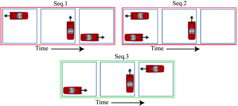
Figure 8: Three sequences of actions. All have equivalent values of $R_{Q,\tau}(\Delta)$; only seq.3 contains a valid U-turn.

We can improve upon the performance of the greedy algorithm in Sec. VI-B1 by exploiting the order of the action components. For example, in the example of a man hopping a subway turnstile, he has to approach the turnstile from the wrong direction, hop over it, and continue. For a car taking a u-turn, it has to approach the intersection, turn across it, and depart the way it came. While these component actions have many valid configurations when examined independently, there is only one order in which they represent the desired full action. This is illustrated in Fig. 8.

In the greedy optimization of Section VI-B1, we ignore the time-ordering that a set of queries contains. The value function $R_{q,\tau}(\Delta)$ does not differentiate between the sequences of actions (Forward, Left, Back) and the sequence of actions (Back, Forward, Left). Intuitively, this should hurt performance - false matches are more likely to appear than were we to exploit this causality. We quantify the improvement upon the performance bounds given in Eq. (5) in Eq. (6).

$$P(Q)=\frac{e^{-N\log{\frac{|D|}{\Delta}}}}{N!}\approx e^{-N\log(\frac{|D|N}{\Delta})}$$ (6)

It is worth highlighting the difference between the two expressions Eq. 5 and Eq. 6. In the latter expression we only need $|D|N$ to be sufficiently large relative to $\Delta$ as opposed to $|D|>\Delta$. Consequently, if we were to account for the order of query components, the probability of randomly matching the user defined query approaches zero even when $\Delta$ scales with the size of the dictionary.

After a user created a query containing a set of $N$ action components (with GUI described in Section VI-A), we search through the inverted index to retrieve $N$ sets of matching locations within the video, one for each action component.

After this pre-processing step, we adapt the Smith-Waterman dynamic programming algorithm [26] , originally developed for gene sequencing, to determine the best set of partial matches in the query. Our algorithm, described in Algorithm 1, operates over the set of matches $m_{\tau,\alpha}\in M(q)$ which contains matches in document $\alpha$ to action component $\tau$ to recover a query that has been distorted. For the purposes of our videos, we consider three types of distortion, namely insertion, deletion and continuation.

(1) Insertion covers documents where we believe the query is happening but there are no partial matches. This can happen if unrelated documents are inserted, if there is a pause in the execution of the activity, or if the activity is obscured.
(2) Deletion covers documents where sections of the query are missing. If a deletion has occurred, one (or more) of the action components in the query will not be present in the video. Deletions can happen because of obscuration, or because somebody does not perform one component of the full action.
(3) Continuation covers documents where we continue to see an action component which we have already seen. This is important because of time distortion; a single action component does not necessarily occur in multiple consecutive documents before the next action component is reached.

Algorithm 1 Dynamic programming (DP) algorithm

1:procedure Search(m, W, T)

2:     $V\leftarrow 0$; $paths\leftarrow\emptyset$; $\tau\leftarrow 1$; $\alpha\leftarrow 1$

3:     while $\tau\leq$ number of documents do

4:         while $\alpha\leq$ number of action components do

5:              $V_{\tau,\alpha}\leftarrow\max\left\{\begin{array}[]{c}0\\ (V_{\tau-1,\alpha-1}+W_{M})*m_{\tau,\alpha}\\ (V_{\tau-1,\alpha}+W_{C})*m_{\tau,\alpha}\\ (V_{\tau-1,\alpha}+W_{D})*(1-m_{\tau,\alpha})\\ (V_{\tau,\alpha-1}+W_{I})*(1-m_{\tau,\alpha})\\ \end{array}\right.$

6:              if Airborne Data then

7:                  $V_{\tau,\alpha}\leftarrow V_{\tau,\alpha}+{\bf 1}_{\phi_{\tau-1,\alpha-1}}(\phi_{\tau,\alpha})*m_{\tau,\alpha}*$

8:                  $W_{S}$

9:              end if

10:              Let $(a,b)$ be the index which was used to

11:              generate the maximum value

12:              if $V_{(\tau,\alpha)}>0$ then

13:                  $paths_{\tau,\alpha}\leftarrow paths_{a,b}\cup(\tau,\alpha)$

14:              else

15:                  $paths_{\tau,\alpha}\leftarrow paths_{a,b}$

16:              end if

17:              $\alpha\leftarrow\alpha+1$

18:         end while

19:         $\tau\leftarrow\tau+1$

20:     end while

21:     $Matches\leftarrow\emptyset$

22:     while $max(V)>T$ do

23:         Let $(a,b)$ be the index of $V$ containing the

24:         maximum value

25:         $Matches\leftarrow Matches\cup paths_{a,b}$

26:         for $\tau,\alpha\in paths_{a,b}$ do

27:              $V_{\tau,\alpha}=0$

28:         end for

29:     end while

30:     Return $Matches$, the set of paths above threshold T

31:end procedure

In addition to the three above distortions, we introduce an extra term to handle the Airborne data. This term adds more score to a match if its Track ID is the same as the ID of the match in the previous document. In Algorithm 1, the track ID of an examined cell is $\phi_{\tau,\alpha}$ where ${\bf 1}_{\phi_{{\tau-1},{\alpha-1}}}(\phi_{\tau,\alpha})$ is an indicator function that returns 1 if $\phi_{\tau,\alpha}=\phi_{\tau-1,\alpha-1}$.

As described in Algorithm 1, to search for a query with $|q|$ action components in a video with $N$ documents, our dynamic programming approach creates an $N\times|q|$ matrix, $V$, which is filled out from the top left to the bottom right. A path through the matrix is defined as a set of adjacent (by an 8-neighborhood) matrix element, where each element of the path represents a hypothetical assignment of an action component taking place in a document. A path containing element $V_{a,b}$ would indicate that action component $b$ occurred in document $a$.

As the matrix is filled out, each element chooses to append itself to the best possible preceding path - which, by definition, ends immediately above it, immediately to the left of it, or both. It stores the resulting value, and a pointer to the preceding element, in the value matrix $V$. When the matrix is fully filled out, the optimal path can be found by starting at the maximal value in the matrix and tracing backwards. In order to find multiple matches, we repeatedly find the maximal value in $V$, the optimal path associated with it, set the values along that path to zero, and repeat until the maximum value in $V$ is below a threshold $T$. This threshold will be called the Retrieval Score Threshold for future references. An example of this matrix, with paths overlaid, is shown in figure 9.

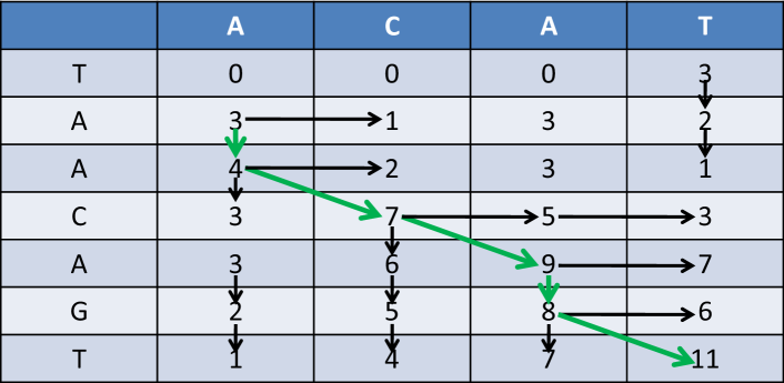
Figure 9: Example of the $V$ matrix. The query is actions A, C, A, T, and the seven documents in the video corpus each contains a single action, T, A, A, C, A, G, T. The values for $W_{I},W_{D},W_{C}$ and $W_{M}$ are $-1,-2,1$ and $3$ in this example. The optimal path, A,A,C,A,G,T, involves an insertion, a continuation and a deletion. It is found by tracing backwards from the maximal element, valued at 11.

For a given penalty on each type of distortion $W_{I},W_{D},W_{C}$ (corresponding to insertion, deletion, and continuation) and a given bonus for each match, $W_{M}$, the DP algorithm (Algorithm 1) is guaranteed to find the set of partial matches which maximizes the sum of the penalties and bonuses over an interval of time. For our queries, we were relatively certain that elements of the query would not be obscured, but we were uncertain about our detection rate on features and how long an event would take. Thus, we set $W_{I}=-1$, $W_{D}=-2$, $W_{C}=1$, and $W_{M}=3$. These values preclude optimal solutions which involve deletions, look for longer sequences that match, and are relatively robust to missed detection. For Airborne footage we also have a bonus $W_{S}$ for a match generated by the same tracklet. In our experiments $W_{S}$ is set to $5$.

We note that because it reasons over specific partial matches, our dynamic programming approach also finds the locations in the video segments where the event occurs, but this is not exploited in the results of this paper.

VII Experimental Results

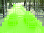
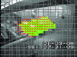
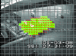
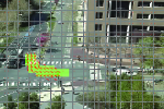
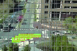
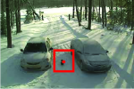
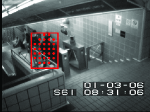
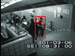
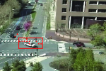
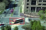
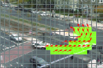
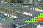
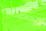
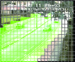
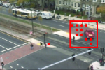
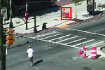
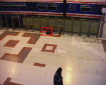
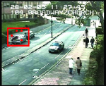
Figure 10: Screen shots of the ten tasks. These images show the search queries (with green ROI) and a retrieve frame (with a red rectangle). The red dots correspond to the tree whose profile fit the query.

Task	Video	Search query	Features	Duration (min.)	Video size	Index size
1	Winter driveway	black cat appearance	color and size	253	6.55 GB	147 KB
2	Subway	people passing turnstiles	motion	79	2.75 GB	2.3 MB
3	Subway	people hopping turnstiles	motion	79	2.75 GB	2.3 MB
4	MIT Traffic	cars turning left	motion	92	10.3 GB	42 MB
5	MIT Traffic	cars turning right	motion	92	10.3 GB	42 MB
6	U-turn	cars making U-turn	motion	3.4	1.97 GB	13.7 MB
7	U-turn	cars turning left, no U	direction	3.4	1.97 GB	13.7 MB
8	Abandoned object	abandoned objects	size and persistence	13.8	682 MB	2.6 MB
9	Abandoned object	abandoned objects	size, persistence and color	13.8	682 MB	2.6 MB
10	PETS	abandoned objects	size and persistence	7.1	1.01 GB	5.63 KB
11	Parked-vehicle	parked vehicles	size and persistence	32
12	Intersection 1	cars moving	tracklets	13.8	1.16 GB	153 KB
13	Beach 1	people walking	tracklets	13.8	529 MB	65 KB

TABLE I: Tasks’ number, videos, search query, associate features, video duration, video size and index size. Videos of Task 12 and 13 have a frame rate of 2 frames per second. Tasks 1, 8, 9, 10, 11, 12 and 13 use compound search operators. The index size can be several orders of magnitude smaller than raw video. Our use of primitive local features implies that index times and index size are both proportional to the number of foreground objects in the video. Consequently, index size tends to be a good surrogate for indexing times.

VII-A Datasets

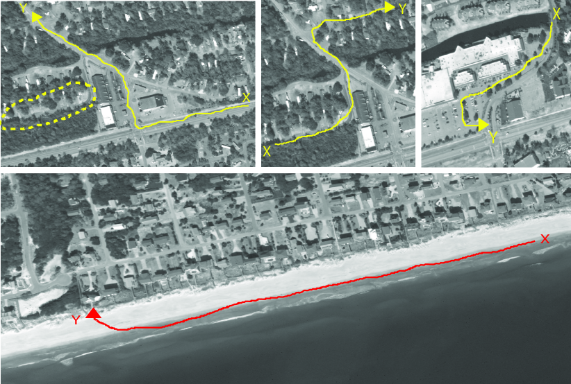
Figure 12: Examples of the examined routes. Routes are shown in yellow/red arrows and they start from point X and end at point Y. Some of the routes undergo strong occlusion (see dashed yellow region, top row, first column, for route in second column) and others undergo many turns (see first row, second and last column).

In order to evaluate performance of the two-step problem formulation, and the DP approach in particular, we tested our two-step approach on eleven CCTV videos and two Airborne videos (see table I, Fig. 10 and Fig. 12). These videos were selected to test the application of this basic approach to multiple domains, as well as to provide a basis for comparison to other algorithms. The Winter driveway, U-Turn and Abandoned object sequences were shot by us, PETS and Parked-vehicle and MIT-traffic come from known databases [3, 1], MIT-traffic was made available to us by Wang et al. [2]; Subway from Adam et al. [5]. Airborne was made available to us by our sponsors.

As listed in Table I, we tested different queries to recover moving objects based on their color, size, direction, activity, persistence and tracklets. We queried for rare and sometimes anomalous events (cat in the snow, illegal U-turns, abandoned objects and people passing turnstile in reverse) as well as usual events (pedestrian counting, car turning at a street light, and car parking). Some videos featured events at a distance MIT-traffic, while others featured people moving close to the camera Subway. We searched for objects, animals, people, and vehicles moving along user-supplied routes.

VII-B Examined Tasks

We examined 11 CCTV footage (see Fig.10 for examples) and 2 Airborne sequences (Fig.12). Once we had defined the queries, manually created a ground-truth list for each task consisting of ranges of frames. Comparison is obtained by computing the intersection of the ranges of frames returned by the search procedure to the range of frames in the ground truth. An event is marked as detected if it appears in the output video and at least 1 partial match hits objects appearing in the event. For airborne footage, we also require that the start and end frames be within 15 frames of the ground truth.

Task	Video	Ground Truth	Greedy True	HDP [16] True	Greedy False	HDP [16] False	Runtime
		(events)	(events found)	(events found)	(events found)	(events found)	(seconds)
1	Winter driveway	3	2	–	1	–	7.5
2	Subway	117	116	114	1	121	0.3
3	Subway	13	11	1	2	33	3.0
4	MIT Traffic	66	61	6	5	58	0.4
5	MIT Traffic	148	135	54	13	118	0.5
6	U-turn	8	8	6	0	23	1.2
7	U-turn	6	5	4	1	14	0.6
8	Abandoned object	2	2	–	0	–	4.8
9	Abandoned object	2	2	–	0	–	13.3
10	PETS	4	4	–	0	–	20.2
11	Parked-vehicle	14	14	–	0	–	12.3

TABLE II: Results for the elevens tasks using greedy optimization and HDP labels. Crossed-out rows correspond to queries for which there was no corresponding topic in the HDP search.

VII-C Comparison with other techniques

For purposes of comparison we implemented two other approaches: the greedy approach described in section VI-B1, and a scene understanding technique based on Hierarchical Dirichlet Processes  [33, 16] described in section VII-C1. For Airborne data, there is also a question of the quality of the tracklet features. As such, we implement our Dynamic Programming approach with a range of features: 1) tracklets from our algorithm, 2) frame to frame motion on the original Airborne footage (ME+DP), 3) frame to frame motion on binary detection masks (MEB+DP), and KLT trajectories (KLT+DP)[24]. We also compare against explicit Track Matching. For a query route, we estimate the common distance between all available tracklets. A tracklet is a match if the common distance is greater than a certain threshold.

VII-C1 HDP Comparison

For the purposes of comparison, we employed high-level search functions based on scene understanding techniques using Hierarchical Dirichelet Processes (HDP)  [33, 16]. At each iteration, the HDP-based learning algorithm assigns each document to one or more high-level activities. This classification is used as input to the next training iteration. Xiang et al.  [33] propose a search algorithm that uses learned topics as high-level semantic queries. The search algorithm is based on the classification outputs from the final HDP training iteration. We compare our method to this HDP-based search algorithm.

Queries are specified as the ideal classification distribution and the search algorithm compares each document distribution over the learned topics against this ideal distribution. Comparison is performed using the relative entropy (Kullback-Leibler divergence) between the two distributions. The Kullback-Leibler divergence gives a measure of distance between the query $q$ and the distribution $p_{j}$ for document $j$ over the $K$ topics:

$$D(q,p_{j})=\sum_{k=1}^{K}q(k)\log\frac{q(k)}{p_{j}(k)}.$$

Query $q$ is created by looking at the ideal documents and assigning to $q$ a uniform distribution over the topics present in them. The search evaluates $D(q,p_{j})$ for each document $j$ and ranks the documents in order of increasing divergence.

VII-D CCTV Results

Results from our greedy-optimization method are displayed in Fig.  10 and summarized in table  II. The comparable results for HDP are summarized below in table  II. The “Ground truth” column of table II indicates the true number of events which exist in the dataset. The “Greedy True” column indicates the number of correct detections (true positives) for our Greedy algorithm and “HDP True” the number of correct detections (true positives) for the HDP-based search  [32]. Likewise, the “Greedy False” and “HDP False” indicate the number of false alarms that were found for those eleven tasks.

Table  II demonstrates the robustness of the two-step method in a wide-array of search applications, outperforming the HDP baseline in detection and false alarm rate. The figures in the table are given for results of total length approximately equal to that of the ground truth. As can be seen from the figures in the table, the absolute detection rate is strong.

From table  II, one can see that HDP-search deals well with search of recurring large-scale activities and poorly otherwise. While several queries could not be executed because of a lack of topics that could be used to model the query, the results nonetheless demonstrate some of the shortcomings of the algorithm. The HDP search scales linearly with the number of documents, an undesirable quality with large datasets. Further, the cost of the training phase is prohibitive (approximately 2 days for the “subway” sequence) and must be paid again every time that more video data is included.

VII-D1 Dynamic Programming

Two of the seven tasks in table I had temporal structure which could be exploited through dynamic programming. In order to demonstrate the potential gain from exploiting this structure, we chose tasks three, four and six and performed dynamic programming using the full query, as well as greedy and HDP search algorithms. The ROC curves for those three scenarios are provided in Fig 11, contrasting dynamic programming with HDP and Greedy Optimization.

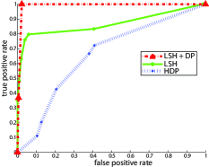
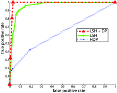
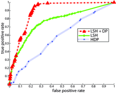
Figure 11: ROC curves for the U-turn, subway and traffic datasets. Both our greedy search and DP significantly outperform scene-understanding methods such as HDP methods [33, 16].

Fig.  11 demonstrates the type of improvement that can be attained by the two-step approach to search. The ROC curves for LSH-based greedy optimization dominate the HDP curves, and there is clear improvement from employing time-ordering with DP. These improvements come as no surprise - HDP is doing a global search, attempting to create a topic for each action. LSH does a compelling local search which is fast and produces low false alarm rate. This is largely due to the global nature of HDP - the topics it discovers are more likely to be common events, so infrequent events such as u-turns and turnstile-hopping pose a problem. Note that the gap between local and global searches narrow on the MIT-traffic dataset, where the event being found (left turns at a light) is a relatively common occurrence.

VII-E Airborne Results

Fig. 13 shows the ROC for the task 12 and 13. Recall that the Retrieval Score Threshold is the minimum path score (generated by Algorithm 1) required in order to declare this path as a correct search result. The points on Fig. 13 represent different Retrieval Score Threshold values for each technique. Those values are equally spaced between the lowest and highest retrieval scores generated by the results. As shown by the generated ROC, our technique outperforms all the other techniques quite noticeably. HDP fails to handle infrequent events. This problem becomes more evident in Task 13 since the beach does not have much activity and hence most queries are considered infrequent.

The accuracy of our tracklets can be quantified by examining Fig. 13. Here our algorithm (see solid red) shows significant improvement over KLT (see solid black) even though Dynamic programming was used in both methods. For cars the improvement accounts for $105\%$ increase in true positives for a false positive rate of $0.2$. For humans improvement is even higher, with $350\%$ increase in true positives for a false positive rate of $0.2$. The higher improvement for humans is expected as KLT is not robust to low contrast features. To quantify the improvements Dynamic Programming brings to the search problem, we compare our technique against ‘Tracking Matching’ (see Fig. 13, dashed black). Here our tracklets are used in both methods. However for ‘Tracking Matching’ we declare a tracklet as a match if the mean absolute error between the query track is within a threshold. Fig. 13 shows a significant improvement in true positives by $500\%$ for both humans and cars at a false positive rate of $0.2$ (see red and dashed black). This shows that Dynamic Programming is capable of significantly boosting search results despite any remaining detection errors.

In terms of computational complexity, HDP is the most expensive. Our approach takes an average of 2.9 seconds to process one frame of Task 12 and 4.32 seconds to process one frame of Task 13. Processing time is computed as the average over $2000$ frames. All experiments are performed on an Intel(R) Core(TM) i7-3820 CPU @ 3.60 GHz 3.60GHz with 16.GB RAM. All algorithms are written in an unoptimized MATLAB code except for the KLT extraction technique which is written in C++ by Shi et al. [24]. Note that our storage procedure spares the burden of having to store all the information. For instance, even though we are extracting as much as $4000$ tracklets for task 12, the size of the generated hash table is around $8000$ times smaller than the size of the actual original data (see Table I).

VII-F Discussion

Our method represents a fundamentally different way of approaching the video search problem. Rather than relying on an abundance of training data or finely-tuned features to differentiate actions of interest from noise, we rely on simple features and causality. In addition to the clear benefits in terms of a run-time which scales sub-linearly with the length of the video corpus, the simple features and hashing approach render the approach robust to user error as well as poor-quality video. Results demonstrate clearly that causality and temporal structure can be powerful tools to reduce false alarms. Another added benefit is how the algorithm scales with query complexity. In our formulation, the more action components in a query, the more likely it is to differentiate itself from noise.

There is, of course, non-temporal structure that we have yet to exploit. Spatial positioning of queries, such as “The second action component must occur to the northeast of the first one”, or “The second action component must be near the first one” is a simple attribute which may further differentiate queries of interest from background noise.

Our method is not void of limitation. One important limitation is that it requires each activity to be made of discrete states, each of which being describable by a simple feature vocabulary. Complex actions like sign language or actions which are to fast or too small to be identified at the atom level will be difficult to search for.

VIII Conclusion

We presented a method that summarizes the dynamic content of a surveillance video in a way that is compatible with arbitrary user-defined queries. We divide the video into documents each containing a series of atoms. These atoms are grouped together into trees all containing a feature list. We used different features for different types of data. For CCTV footage we used size, color, direction and persistence of the moving objects. For Airborne footage we used tracklets of examined objects. Here a viterbi approach for tracklet generation is used. The coordinates of the features trees are then stored into a hash-table based feature index. Hash functions group trees whose content is similar. In this way, search becomes a simple lookup as user-specified queries are converted into a table index. Our method has many advantages. First, because of the indexing strategy, our search engine has a complexity of $O(1)$ for finding partial matches. Second, the index requires minimal storage. Third, our method requires only local processing, making it suitable for facing constant data renewal. This makes it simple to implement and easy to adjust. Fourth, our method summarizes the entire video, not just the predominant modes of activity: it can retrieve any combination of rare, abnormal and recurrent activities.

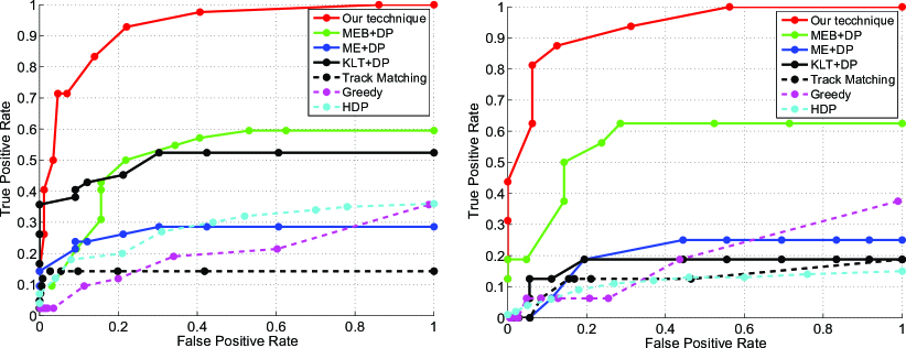
Figure 13: ROC for the examined airborne data. Here results for routes generated by cars and humans are shown on the left and right respectively. The points on the graph represent different values for Retrieval Score Threshold.

References

- [1] i-lids. computervision.wikia.com/wiki/I-LIDS.
- [2] Mit traffic. people.csail.mit.edu/xgwang/HBM.html.
- [3] Pets 2006. http://ftp.pets.rdg.ac.uk/.
- [4] M. Abramowitz and I. A. Stegun. Handbook of Mathematical Functions. Dover, New York, 1970.
- [5] A. Adam, E. Rivlin, I. Shimshoni, and D. Reinitz. Robust real-time unusual event detection using multiple fixed-location monitors. IEEE Trans. PAMI, 30(3):555–560, 2008.
- [6] G. Baugh and A. Kokaram. A Viterbi tracker for local features . In Proc. SPIE Vis. Comm. and Image Process., pages 7543–23, 2009.
- [7] Y. Benezeth, P-M. Jodoin, B. Emile, H. Laurent, and C. Rosenberger. Comparative study of background subtraction algorithms. J. of Elec. Imaging, 19(3):1–12, 2010.
- [8] B.Horn and B. Schunck. Determining optical flow. Artif. Intell., 17(1-3):185–203, 1981.
- [9] C. Bouman. Cluster: An unsupervised algorithm for modeling gaussian mixtures. Technical report, Purdue University, 1998.
- [10] S. Calderara, R. Cucchiara, and A. Prati. A distributed outdoor video surveillance system for detection of abnormal people trajectories. In Proc. IEEE Conf. on Dist. Smart Cameras, pages 364–371, 2007.
- [11] R. Emonet, J. Varadarajan, and J-M Odobez. Temporal analysis of motif mixtures using dirichlet processes. IEEE Trans. PAMI, 36(1):140–156, 2014.
- [12] A. Gionis, Piotr Indyk, and R. Motwani. Similarity search in high dimensions via hashing. In Proc. Int. Conf. on Very Large Data Bases, pages 518–529, 1999.
- [13] L. Gorelick, M. Blank, E. Shechtman, M. Irani, and R. Basri. Actions as space-time shapes. IEEE Trans. PAMI, 29(12):2247–2253, 2007.
- [14] M. Hoferlin, B. Hoferlin, G. Heidemann, and D. Weiskopf. Interactive schematic summaries for faceted exploration of surveillance video. IEEE Trans. Multimedia, 15:908–920, 2013.
- [15] E. Jouneau and C. Carincotte. Particle-based tracking model for automatic anomaly detection. In Proc. IEEE Int. Conf. Image Processing, pages 513–516, 2011.
- [16] D. Kuettel, M. Breitenstein, L. Gool, and V. Ferrari. What’s going on? discovering spatio-temporal dependencies in dynamic scenes. In Proc. IEEE Comp. Vis. Pat. Rec., pages 1951–1958, 2010.
- [17] H. Lee, A. Smeaton, N. O’Connor, and N. Murphy. User-interface to a cctv video search system. In IEE Int Symp on Imaging for Crime Detec. and Prev., pages 39–43, 2005.
- [18] S. Little, K. Clawson, A. Mereu, and A. Rodriguez. dentifying and addressing challenges for search and analysis of disparate surveillance video archives. In In proc of ICICPD, 2013.
- [19] J. Meessen, M. Coulanges, X. Desurmont, and J-F Delaigle. Content-based retrieval of video surveillance scenes. In MRCS, pages 785–792, 2006.
- [20] F. Pitié, S-A. Berrani, R. Dahyot, and A. Kokaram. Off-line multiple object tracking using candidate selection and the viterbi algorithm. In Proc. IEEE Int. Conf. Image Processing, 2005.
- [21] I. Pruteanu-Malinici and L. Carin. Infinite hidden markov models for unusual-event detection in video. IEEE Trans. Image Process., 17(5):811–821, 2008.
- [22] V. Saligrama, J. Konrad, and P.-M. Jodoin. Video anomaly identification: A statistical approach. IEEE Signal Process. Mag., 27:18–33, 2010.
- [23] E. Shechtman and M. Irani. Space-time behavior based correlation or how to tell if two underlying motion fields are similar without computing them? IEEE Trans. PAMI, 29(11):2045–2056, 2007.
- [24] Jianbo Shi and Carlo Tomasi. Good features to track. In Proc. IEEE Comp. Vis. Pat. Rec., pages 593 – 600, 1994.
- [25] C. Simon, J. Meessen, and C. DeVleeschouwer. Visual event recognition using decision trees. Multimedia Tools and App., 2009.
- [26] T.F. Smith and M.S. Waterman. Identification of common molecular subsequences. J. of Molecular Biology, 147:195–197, 1981.
- [27] E. Stringa and C. Regazzoni. Content-based retrieval and real time detection from video sequences acquired by surveillance systems. In Proc. IEEE Int. Conf. Image Processing, pages 138–142, 1998.
- [28] C. Sujatha and U. Mudenagudi. A study on keyframe extraction methods for video summary. In in proc of ICCICS, pages 73–77, 2011.
- [29] J. Thornton, J. Baran-Gale, D. Butler, M. Chan, and H. Zwahlen. Person attribute search for large-area video surveillance. In IEEE Int. Conf. on Tech. for Homeland Security., pages 55–61, 2011.
- [30] Y-L. Tian, A. Hampapur, L. Brown, R. Feris, M. Lu, A. Senior, C-F. Shu, and Y. Zhai. Event detection, query, and retrieval for video surveillance. In Zongmin Ma, editor, Artificial Intelligence for Maximizing Content Based Image Retrieval. Information Science Reference, 2008.
- [31] H. Veeraraghavan, N. Papanikolopoulos, and P. Schrater. Learning dynamic event descriptions in image sequences. In Proc. IEEE Comp. Vis. Pat. Rec., pages 1–6, 2007.
- [32] X. Wang, X. Ma, and E.Grimson. Unsupervised activity perception in crowded and complicated scenes using hierarchical bayesian models. IEEE Trans. PAMI, 31(3):539–555, 2009.
- [33] T. Xiang and S. Gong. Video behavior profiling for anomaly detection. IEEE Trans. PAMI, 30(5):893–908, 2008.
- [34] Y. Yang, B. Lovell, and F. Dadgostar. Content-based video retrieval (cbvr) system for cctv surveillance videos. In Proc of Dig. Img. Comp. Tech. and App., pages 183–187, 2009.
- [35] C. Yeo, P. Ahammad, K. Ramchandran, and S. Sastr. High speed action recognition and localization in compressed domain videos. IEEE Trans. Circuits Syst. Video Technol., 18(8):1006 – 1015, 2008.
- [36] A. Yilmaz and M. Shah. A differential geometric approach to representing the human actions. Comput. Vis. Image Und., 109(3):335–351, 2008.
- [37] X. Zhu, X. Wu, A. Elmagarmid, Z. Feng, and L. Wu. Video data mining:semantic indexing and event detection from the association perspective. IEEE Trans. Know Data En, 17:665–677, 2005.