Fast symmetric factorization of hierarchical matrices with applications

Abstract

We present a fast direct algorithm for computing symmetric factorizations, i.e. $A=WW^{T}$, of symmetric positive-definite hierarchical matrices with weak-admissibility conditions. The computational cost for the symmetric factorization scales as $\mathcal{O}(n\log^{2}n)$ for hierarchically off-diagonal low-rank matrices. Once this factorization is obtained, the cost for inversion, application, and determinant computation scales as $\mathcal{O}(n\log n)$. In particular, this allows for the near optimal generation of correlated random variates in the case where $A$ is a covariance matrix. This symmetric factorization algorithm depends on two key ingredients. First, we present a novel symmetric factorization formula for low-rank updates to the identity of the form $I+UKU^{T}$. This factorization can be computed in $\mathcal{O}(n)$ time if the rank of the perturbation is sufficiently small. Second, combining this formula with a recursive divide-and-conquer strategy, near linear complexity symmetric factorizations for hierarchically structured matrices can be obtained. We present numerical results for matrices relevant to problems in probability & statistics (Gaussian processes), interpolation (Radial basis functions), and Brownian dynamics calculations in fluid mechanics (the Rotne-Prager-Yamakawa tensor).

1 Introduction

This article describes a computationally efficient method for constructing the symmetric factorization of large dense matrices. The symmetric factorization of large dense matrices is important in several fields, including, among others, data analysis [14, 33, 41], geostatistics [32, 40], and hydrodynamics [16, 26]. For instance, several schemes for multi-dimensional Monte Carlo simulations require drawing covariant realizations of multi-dimensional random variables. In particular, in the case where the marginal distribution of each random variable is normal, the covariant samples can be obtained by applying the symmetric factor of the corresponding covariance matrix to independent normal random vectors. The symmetric factorization of a symmetric positive-definite matrix is given as the factor $W$ in $A=W^{T}W$. One of the major computational issues in dealing with large covariance matrices is that they are often dense. Conventional methods of obtaining a symmetric factorization based on the Cholesky decomposition are expensive, since the computational cost scales as $\mathcal{O}(n^{3})$ for an $n\times n$ matrix. Relatively recently, however, it has been observed that large dense (full-rank) covariance matrices can be efficiently represented using hierarchical decompositions [5, 6, 7, 35, 28, 13]. Taking advantage of this underlying structure, we derive a novel symmetric factorization for large dense Hierarchical Off-Diagonal Low-Rank (HODLR) matrices that scales as $\mathcal{O}(n\log^{2}n)$. That is to say, for a given $n\times n$ matrix $A$, we decompose it as $A=WW^{T}$. A major difference of our scheme versus the Cholesky decomposition is the fact that the matrix $W$ is no longer a triangular matrix. In fact, the algorithm of this paper constructs the matrix $W$ as a product of matrices which are block low-rank updates of the identity matrix. The cost of applying the resulting factor $W$ to a vector scales as $\mathcal{O}(n\log n)$.

Hierarchical matrices were first introduced in the context of integral equations [20, 23] arising out of elliptic partial differential equations and potential theory. Since then, it has been observed that large classes of dense matrices arising out of boundary integral equations [45, 27, 4], dense fill-ins in finite element matrices [42, 8], radial basis function interpolation [3], kernel density estimation in machine learning, covariance structure in statistical models [13], Bayesian inversion [3, 6, 7], Kalman filtering [28], and Gaussian processes [5] can be efficiently represented as data-sparse hierarchical matrices. After a suitable ordering of columns and rows, these matrices can be recursively sub-divided using a tree structure. Certain sub-matrices at each level in the tree can then be well-represented by low-rank matrices. We refer the readers to [20, 23, 18, 21, 10, 12, 11, 2, 4] for more details on these matrices. Depending on the tree structure and low-rank approximation technique, different hierarchical decompositions exist. For example, the original fast multipole method [19] (from now on abbreviated as FMM) accelerates the calculation of long-range gravitational forces for $n$-body problems by hierarchically compressing (via a quad- or oct-tree) certain interactions in the associated matrix operator using analytical low-rank considerations. The low-rank sparsity structure of these hierarchical matrices can be exploited to construct fast dense linear algebra schemes, including direct inversion, determinant computation, symmetric factorization, etc. Broadly speaking, different hierarchical matrices can be divided into categories based on two main criteria: (i) Admissibility (strong and weak), (ii) Nested low-rank basis. The admissibility criterion identifies and specifies sub-blocks of the hierarchical matrix that can be represented as a low-rank matrix, while the nested low-rank basis enables additional compression of the low-rank sub-matrices, by assuming that the low-rank basis of a parent can be obtained using the low-rank basis of its children. (For instance, the difference between “FMMs” and “tree-codes” is that there are no translation operators between one level to the other in the case of tree-codes). A detailed analysis of these different hierarchical structures is provided in [2, 4]. We also refer readers to [24] for a thorough discussion and analysis of hierarchical matrices with weak admissibility criteria.

Most of the existing results relevant to the symmetric factorization of low-rank modifications to the identity are based on rank $1$ or rank $r$ modifications to the Cholesky factorization, which are computationally expensive, i.e., their scaling is at least $\mathcal{O}(rn^{2})$. We do not seek to review the entire literature here, except to direct the readers to a few references [36, 25, 17, 9].

The scheme presented here for HODLR matrices scales as $\mathcal{O}(n\log^{2}n)$. The algorithm also extends to other hierarchical structures naturally. However, for matrices with strong admissibility criteria, the algorithm scales depending on the underlying dimension as illustrated in Section 5. Xia and Gu [43] also discuss a Cholesky factorization for hierarchical matrices (Hierarchically Semi-Separable matrices to be specific, which are also termed as $\mathcal{H}^{2}$ matrices with weak admissibility criteria [22]). Once the HSS factorization is computed, their algorithm scales as $\mathcal{O}(n)$. As presented, the cost of constructing the HSS representation in their article scales as $\mathcal{O}(n^{2})$. It is possible to reduce the computational cost of forming an HSS representation to $\mathcal{O}(n)$, for instance, using randomized algorithms as discussed in [31]. The HODLR matrices have a weaker assumption on the off-diagonal blocks as opposed to HSS matrices and therefore algebraic techniques for assembling HODLR matrices are simpler and easier. A comparison of the computational cost for each step of our algorithm and the algorithm by Xia and Gu [43] is presented in Table 1.

Table 1: Computational cost of each of the significant step in symmetric factorization

	Matrix type	Algorithm	Assembly	Factorization	Solve
Our method	HODLR	Symmetric factorization	$\mathcal{O}(n\log n)$	$\mathcal{O}(n\log^{2}n)$	$\mathcal{O}(n\log n)$
Xia and Gu [43]	HSS	Cholesky	$\mathcal{O}(n^{2})$	$\mathcal{O}(n)$	$\mathcal{O}(n)$

The paper is organized as follows: Section 3 contains the key idea behind the algorithm discussed in this paper: a fast, symmetric factorization for low-rank updates to the identity. Section 4 extends the formula of Section 3 to a nested product of block low-rank updates to the identity. The details of the compatibility of this structure with HODLR matrices is discussed. Section 5 contains numerical results (accuracy and complexity scaling) of applying the factorization algorithms to matrices relevant to problems in statistics, interpolation and hydrodynamics. Section 6 summarizes the previous results and discusses further extensions and areas of ongoing research. The algorithm discussed in this article has been implemented in C++ (parallelized using OpenMP) and the implementation is made available at https://gitlab.com/SAFRAN/HODLR.

2 Acknowledgements

The research supported in part by the Air Force Office of Scientific Research under NSSEFF Program Award FA9550-10-1-0180. SA was also supported by the INSPIRE faculty award [DST/INSPIRE/04/2014/001809] by the Department of Science & Technology, India and the startup grant provided by the Indian Institute of Science.

3 Symmetric Factorization of low-rank update

Almost all of the hierarchical factorizations are typically based on incorporating low-rank perturbations in a hierarchical manner. In this section, we briefly discuss some well-known identities which allow for the rapid inversion and determinant computation of low-rank updates to the identity matrix.

3.1 The Sherman-Morrison-Woodbury formula

If the inverse of a matrix $A\in\mathbb{R}^{n\times n}$ is already known, then the inverse of subsequent low-rank updates, for $U,V\in\mathbb{R}^{n\times p}$ and $C\in\mathbb{R}^{p\times p}$, can be calculated as

(1) $$\left(A+UCV^{T}\right)^{-1}=A^{-1}-A^{-1}U\left(C^{-1}+V^{T}A^{-1}U\right)^{-1}V^{T}A^{-1},$$

where we should point out that the quantity $V^{T}U$ is only a $p\times p$ matrix. This formula is known as the Sherman-Morrison-Woodbury (SMW) formula. Further simplifying, in the case where $A=I$, we have

(2) $$\left(I+UCV^{T}\right)^{-1}=I-U(C^{-1}+V^{T}U)^{-1}V^{T}.$$

Note that the SMW formula shows that the inverse of a low-rank perturbation to the identity matrix is also a low-rank perturbation to the identity matrix. Furthermore, the row-space and column-space of the low-rank perturbation and its inverse are the same. The main advantage of Equation (2) is that if $p\ll n$, we can obtain the inverse (or equivalently solve a linear system) of a rank $p$ perturbation of an $n\times n$ identity matrix at a computational cost of $\mathcal{O}(p^{2}n)$. In general, if $B\in\mathbb{R}^{n\times n}$ is a low-rank perturbation of $A\in\mathbb{R}^{n\times n}$, then the inverse of $B$ is also a low-rank perturbation of the inverse of $A$.

It is also worth noting that if $A$ and $B$ are well-conditioned, then the Sherman-Morrison-Woodbury formula is numerically stable [46]. The SMW formula has found applications in, to name a few, Kalman filters [30], recursive least-squares [15], and fast direct solvers for hierarchical matrices [3, 37, 29].

3.2 Sylvester’s determinant theorem

Calculating the determinant of an $n\times n$ matrix $A$, classically, using a cofactor expansions requires $\mathcal{O}(n!)$ operations. However, this can be reduced to $\mathcal{O}(n^{3})$ by first computing the $LU$ or eigenvalue decomposition of the matrix. Recently [5], it was shown that the determinant of HODLR matrices could be calculated in $\mathcal{O}(n\log n)$ time using Sylvester’s determinant theorem [1], a formula relating the determinant of a low-rank update of the identity to the determinant of a smaller matrix. Determinants of matrices are very important in probability and statistics, in particular in Bayesian inference, as they often serve as the normalizing factor in likelihood calculations and in the evaluation of the conditional evidence.

Sylvester’s determinant theorem states that for $A,B\in\mathbb{R}^{n\times p}$,

(3) $$\det\left(I+AB^{T}\right)=\det\left(I+B^{T}A\right),$$

where the determinant on the right hand side is only of a $p\times p$ matrix. Hence, the determinant of a rank $p$ perturbation to an $n\times n$ identity matrix, where $p\ll n$, can be computed at a computational cost of $\mathcal{O}(p^{2}n)$. This formula has recently found applications in Bayesian statistics for computing precise values of Gaussian likelihood functions (which depend on the determinant of the corresponding covariance matrix) [5] and computing the determinant of large matrices in random matrix theory [39].

3.3 Symmetric factorization of a low-rank update

In the spirit of the Sherman-Morrison-Woodbury formula and Sylvester’s determinant theorem, we now obtain a formula that enables the symmetric factorization of a rank $p$ perturbation to the $n\times n$ identity at a computational cost of $\mathcal{O}(p^{2}n)$. In particular, for a symmetric positive-definite (from now on abbreviated as SPD) matrix of the form $I+UKU^{T}$, where $I$ is an $n\times n$ identity matrix, $U\in\mathbb{R}^{n\times p}$, $K\in\mathbb{R}^{p\times p}$, and $p\ll n$, we obtain the factorization

(4) $$I+UKU^{T}=WW^{T}.$$

We now state this as the following theorem.

Theorem 1.

For rank $p$ matrices $U\in\mathbb{R}^{n\times p}$ and $K\in\mathbb{R}^{p\times p}$, if the matrix $I+UKU^{T}$ is SPD then it can be symmetrically factored as

(5) $$I+UKU^{T}=\left(I+UXU^{T}\right)\left(I+UXU^{T}\right)^{T}$$

where $X$ is obtained as

(6) $$X =L^{-T}\left(M-I\right)L^{-1},$$

the matrix $L$ is the symmetric factor of $U^{T}U$, and $M$ is the symmetric factor of $I+L^{T}KL$, i.e.,

(7) $$LL^{T} =U^{T}U,$$

(8) $$MM^{T} =I+L^{T}KL.$$

We first prove two lemmas related to the construction of $X$ in Equation (6), which directly lead to the proof of Theorem 1. In the subsequent discussion, we will assume the following unless otherwise stated:

1. $I$ is the identity matrix.

2. $p\ll n$.

3. $U\in\mathbb{R}^{n\times p}$ is of rank $p$.

4. $K\in\mathbb{R}^{p\times p}$ is of rank $p$.

5. $I+UKU^{T}$ is SPD.

It is easy to show that the last item implies that the matrix $K$ is symmetric. The first lemma we prove relates the positivity of the smaller matrix $I+L^{T}KL\in\mathbb{R}^{p\times p}$ to the positivity of the larger $n\times n$ matrix, $I+UKU^{T}$.

Lemma 2.

Let $LL^{T}$ denote a symmetric factorization of $U^{T}U$, where $L\in\mathbb{R}^{p\times p}$. If the matrix $I+UKU^{T}$ is SPD (semi-definite), then $I+L^{T}KL$ is also SPD (semi-definite).

Proof.

To prove that $I+L^{T}KL$ is SPD, it suffices to prove that given any non-zero $\boldsymbol{y}\in\mathbb{R}^{p}$, we have $\boldsymbol{y}^{T}(I+L^{T}KL)\boldsymbol{y}>0$. Note that since $U$ is full rank, the matrix $U^{T}U$ is invertible. We now show that given any $\boldsymbol{y}\in\mathbb{R}^{p}$, there exists an $\boldsymbol{x}\in\mathbb{R}^{n}$ such that $\boldsymbol{y}^{T}(I+L^{T}KL)\boldsymbol{y}=\boldsymbol{x}^{T}(I+UKU^{T})\boldsymbol{x}$. This will enable us to conclude that $I+L^{T}KL$ is positive definite since $I+UKU^{T}$ is positive-definite. In fact, we will directly construct $\boldsymbol{x}\in\mathbb{R}^{n}$ such that $\boldsymbol{y}^{T}(I+L^{T}KL)\boldsymbol{y}=\boldsymbol{x}^{T}(I+UKU^{T})\boldsymbol{x}$.

Let us begin by choosing $\boldsymbol{x}=U(U^{T}U)^{-1}L\boldsymbol{y}$. Then, the following two criteria are met:

1. $\|\boldsymbol{x}\|_{2}=\|\boldsymbol{y}\|_{2}$.

2. $\boldsymbol{x}^{T}UKU^{T}\boldsymbol{x}=\boldsymbol{y}^{T}L^{T}KL\boldsymbol{y}$.

Expanding the norm of $\boldsymbol{x}$ we have:

(9) $$\|\boldsymbol{x}\|_{2}^{2} =\boldsymbol{y}^{T}L^{T}(U^{T}U)^{-T}\overbrace{U^{T}U(U^{T}U)^{-1}}^{I}L\boldsymbol{y}$$

(10) $$=\boldsymbol{y}^{T}L^{T}(U^{T}U)^{-T}L\boldsymbol{y}$$

(11) $$=\boldsymbol{y}^{T}L^{T}(LL^{T})^{-T}L\boldsymbol{y}$$

(12) $$=\boldsymbol{y}^{T}L^{T}(L^{-T}L^{-1})L\boldsymbol{y}$$

(13) $$=\|\boldsymbol{y}\|_{2}^{2}.$$

This proves criteria (i). Furthermore, by our choice of $\boldsymbol{x}$, we also have that $U^{T}\boldsymbol{x}=L\boldsymbol{y}$. Therefore,

(14) $$\boldsymbol{x}^{T}UKU^{T}\boldsymbol{x} =(U^{T}\boldsymbol{x})^{T}K(U^{T}\boldsymbol{x})$$

(15) $$=(L\boldsymbol{y})^{T}K(L\boldsymbol{y})$$

(16) $$=\boldsymbol{y}^{T}L^{T}KL\boldsymbol{y}.$$

This proves criteria (ii). From the above, we can now conclude that

(17) $$\boldsymbol{y}^{T}(I+L^{T}KL)\boldsymbol{y}=\boldsymbol{x}^{T}(I+UKU^{T})\boldsymbol{x}.$$

Hence, if $I+UKU^{T}$ is SPD, so is $I+L^{T}KL$. An identical calculation proves the positive semi-definite case. ∎

We now state and prove a lemma required for solving a quadratic matrix equation that arises in the subsequent factorization scheme.

Lemma 3.

A solution $X$ to the quadratic matrix equation

(18) $$XLL^{T}X^{T}+X+X^{T}=K$$

with $L,K\in\mathbb{R}^{p\times p}$ and $L$ a full rank matrix is given by

(19) $$X=L^{-T}(M-I)L^{-1},$$

where $M\in\mathbb{R}^{p\times p}$ is a symmetric factorization of $I+L^{T}KL$, that is, $MM^{T}=I+L^{T}KL$.

Proof.

First note that from Lemma 2, since $I+L^{T}KL$ is positive-definite, the symmetric factorization $I+L^{T}KL=MM^{T}$ exists. Now the easiest way to check if Equation (19) satisfies Equation (18) is to plug in the value of $X$ from Equation (19) in Equation (18). This yields:

(20) $$XLL^{T}X^{T} =L^{-T}(M-I)\overbrace{L^{-1}L}^{I}L^{T}(L^{-T}(M-I)L^{-1})^{T}$$

(21) $$=L^{-T}(M-I)\underbrace{L^{T}L^{-T}}_{I}(M-I)^{T}L^{-1}.$$

Further simplifying the expression, we have:

(22) $$XLL^{T}X^{T} =L^{-T}(M-I)(M^{T}-I)L^{-1}$$

(23) $$=L^{-T}(MM^{T}-M-M^{T}+I)L^{-1}$$

(24) $$=L^{-T}(2I-M-M^{T}+L^{T}KL)L^{-1}$$

(25) $$=L^{-T}(I-M)L^{-1}+L^{-T}(I-M^{T})L^{-1}+K$$

(26) $$=-X-X^{T}+K.$$

Therefore, we have that $XLL^{T}X^{T}+X+X^{T}=K$ ∎

We are now ready to prove the main result, Theorem 1.

Proof.

(Proof of Theorem 1 ) The proof follows immediately from the previous two lemmas. With $X$ and $L$ as previously defined as in Equation (6), we have

(27) $$(I+UXU^{T})(I+UXU^{T})^{T} =I+U(X+X^{T}+XU^{T}UX^{T})U^{T}$$

(28) $$=I+U(X+X^{T}+XLL^{T}X^{T})U^{T}.$$

Since $X=L^{-T}(M-I)L^{-1}$ and $MM^{T}=I+L^{T}KL$, from Lemma 3 we have that $X+X^{T}+XLL^{T}X^{T}=K$. Substituting in the previous equation, we get

(29) $$(I+UXU^{T})(I+UXU^{T})^{T}=I+UKU^{T}.$$

This proves the symmetric factorization. ∎

Remark 4.

A slightly more numerically stable variant of factorization (5) is:

(30) $$I+UKU^{T}=\left(I+Q\tilde{X}Q^{T}\right)\left(I+Q\tilde{X}Q^{T}\right)^{T},$$

where $Q$ is a unitary matrix such that $U=QR$.

Remark 5.

Even though the previous theorem only addresses the symmetric factorization problem with no restrictions of the factors being symmetric (i.e., $W=W^{T}$), we can also easily obtain a square-root factorization in a similar manner. By this we mean that for a given symmetric positive-definite matrix $A$, one can obtain a symmetric matrix $G$ such that $G^{2}=A$. The key ingredient is obtaining a square-root factorization of a low-rank update to the identity:

(31) $$I+UKU^{T}=(I+UXU^{T})^{2},$$

where $X$ is a symmetric matrix and satisfies

(32) $$K=X(UU^{T})X+2X.$$

The solution to Equation (32) is given by

(33) $$X=L^{-1}(M-I)L^{-1},$$

where $L$ and $M$ are symmetric square-roots of $U^{T}U$ and $I+LKL$:

(34) $$L^{2} =U^{T}U.$$

(35) $$M^{2} =I+LKL.$$

These factorizations can easily be obtained via a singular value or eigenvalue decomposition. This can then be combined with the recursive divide-and-conquer strategy discussed in the next section to yield an $\mathcal{O}(n\log^{2}n)$ algorithm for computing square-roots of HODLR matrices.

Theorem 1 has the two following useful corollaries.

Corollary 6.

If $p=1$, i.e., the perturbation to the identity in Equation (5) is of rank $1$, then

(36) $$I+\boldsymbol{u}\boldsymbol{u}^{T}=(I+\alpha\boldsymbol{u}\boldsymbol{u}^{T})(I+\alpha\boldsymbol{u}\boldsymbol{u}^{T}),$$

where $\alpha=\dfrac{\sqrt{1+\|\boldsymbol{u}\|_{2}^{2}}-1}{\|\boldsymbol{u}\|_{2}^{2}}$.

This result can also be found in [17]. Corollary 7 extends low-rank updates to SPD matrices other than the identity.

Corollary 7.

Given a symmetric factorization of the form $WW^{T}$, where the inverse of $W$ can be applied fast (i.e., the linear system $W\boldsymbol{x}=\boldsymbol{y}$ can be solved fast), then a symmetric factorization of a SPD matrix of the form $WW^{T}+UKU^{T}$, where $U\in\mathbb{R}^{n\times p}$ and $p\ll n$, can also be obtained fast. For instance, if the linear system $W\boldsymbol{x}=\boldsymbol{y}$ can be solved at a computational cost of $\mathcal{O}(n)$, then the symmetric factorization $W(I+\tilde{U}X\tilde{U}^{T})(I+\tilde{U}X\tilde{U}^{T})^{T}W^{T}$ can also be obtained at a computational cost of $\mathcal{O}(n)$.

A numerical example demonstrating Corollary 7 is contained in Section 5.1.

Note that the factorizations in Equations (5) and (30) are similar to the Sherman-Morrison-Woodbury formula; in each case, the symmetric factor is a low-rank perturbation to the identity. Furthermore, the row-space and column-space of the perturbed matrix are the same as the row-space and column-space of the symmetric factors. Another advantage of the factorization in Equations (5) and (30) is that the storage cost and the computational cost of applying the factor to a vector, which is of significant interest as indicated in the introduction, scales as $\mathcal{O}(pn)$.

We now describe a computational algorithm for finding the symmetric factorization described in Theorem 1. Algorithm 1 lists the individual steps in computing the symmetric factorization and their associated computational cost. The only computational cost is in computing the matrix $X$ in Equation (5). Note that the dominant cost is the matrix-matrix product of an $p\times n$ matrix with a $n\times p$ matrix. The rest of the steps are performed on a lower $p$-dimensional space.

Algorithm 1 Symmetric factorization of $I+UKU^{T}$.

Step	Computation	Cost
$1$	Calculate $A=U^{T}U\in\mathbb{R}^{p\times p}$	$\mathcal{O}(p^{2}n)$
$2$	Factor $A$ as $LL^{T}$, where $L\in\mathbb{R}^{p\times p}$	$\mathcal{O}(p^{3})$
$3$	Calculate $T=I+L^{T}KL\in\mathbb{R}^{p\times p}$	$\mathcal{O}(p^{3})$
$4$	Factorize $T$ as $MM^{T}$, where $M\in\mathbb{R}^{p\times p}$	$\mathcal{O}(p^{3})$
$5$	Calculate $X=L^{-T}(M-I_{p})L^{-1}\in\mathbb{R}^{p\times p}$	$\mathcal{O}(p^{3})$

Algorithm 1 can be made more stable by first performing a $QR$ decomposition of the matrix $U$ as indicated in Equation (30). Here, the dominant cost is in obtaining the $QR$ factorization of the matrix $U$. This is described in Algorithm 2.

Algorithm 2 Stable version of symmetric factorization of $I+UKU^{T}$.

Step	Computation	Cost
$1$	$QR$ decompose $U=QR$, where $Q\in\mathbb{R}^{n\times p}$ and $R\in\mathbb{R}^{p\times p}$	$\mathcal{O}(p^{2}n)$
$2$	Calculate $T=I+RKR^{T}\in\mathbb{R}^{p\times p}$	$\mathcal{O}(p^{3})$
$3$	Factorize $T$ as $MM^{T}$, where $M\in\mathbb{R}^{p\times p}$	$\mathcal{O}(p^{3})$
$4$	Calculate $X=M-I\in\mathbb{R}^{p\times p}$	$\mathcal{O}(p)$

Remark 8.

If $U$ is rank deficient, then the reduced-rank $QR$ decomposition must be computed. Algorithm 2 proceeds accordingly with a smaller internal rank $\tilde{p}$.

Remark 9.

Note that if $U$ is unitary, then Equation (6) reduces to $X=M-I$ and Equation (8) reduces to $MM^{T}=I+K$. Note that in our case $K$ is of the form

$$K=\begin{bmatrix}0&\tilde{K}^{T}\\ \tilde{K}&0\end{bmatrix}$$

Hence, the Cholesky decomposition of $I+K$ is of the form

$$I+K=\begin{bmatrix}I&0\\ \tilde{K}&D\end{bmatrix}\begin{bmatrix}I&\tilde{K}^{T}\\ 0&D^{T}\end{bmatrix}$$

where we need $DD^{T}=I-\tilde{K}\tilde{K}^{T}$. Hence, to find the Cholesky decomposition of $I+K$, it suffices to find the Cholesky decomposition of $I-\tilde{K}\tilde{K}^{T}$. Note that matrix $I-\tilde{K}\tilde{K}^{T}$ is half the size of the matrix $I+K$.

Remark 10.

From the above, we also note that if $U$ is unitary, we then have

(37) $$\det(M) =\det(D)$$

This inturn gives us that

(38) $$\det(I+UKU^{T}) =\det(I+UXU^{T})^{2}=\det(I+X)^{2}=\det(M)^{2}=\det(D)^{2}$$

4 Symmetric Factorization of HODLR matrices

In this section, we extend the symmetric factorization formula of the previous section to a class of hierarchically structured matrices, known as Hierarchical Off-Diagonal Low-Rank matrices.

4.1 Hierarchical Off-Diagonal Low Rank matrices

There exists a variety of hierarchically structured matrices depending on the particular matrix, choice of recursive sub-division (inherent tree structure), and low-rank sub-block compression technique (refer to Chapter 3 of [2] for more details). In this article, we will focus on a specific class of matrices known as Hierarchical Off-Diagonal Low-Rank (HODLR) matrices. Furthermore, since this article deals with SPD matrices, we shall restrict our attention to SPD-HODLR matrices. We first briefly review the HODLR matrix structure.

A matrix $A\in\mathbb{R}^{n\times n}$ is termed a $2$-level HODLR matrix if it can be written in the form:

(39) $$A =\begin{bmatrix}A_{1}^{(1)}&U_{1}^{(1)}K_{1,2}^{(1)}V_{2}^{(1)^{T}}\\ U_{2}^{(1)}K_{2,1}^{(1)}V_{1}^{(1)^{T}}&A_{2}^{(1)}\end{bmatrix}$$

(40) $$=\begin{bmatrix}\begin{bmatrix}A_{1}^{(2)}&U_{1}^{(2)}K_{1,2}^{(2)}V_{2}^{(2)^{T}}\\ U_{2}^{(2)}K_{2,1}^{(2)}V_{1}^{(2)^{T}}&A_{2}^{(2)}\end{bmatrix}&U_{1}^{(1)}K_{1,2}^{(1)}V_{2}^{(1)^{T}}\\ U_{2}^{(1)}K_{2,1}^{(1)}V_{1}^{(1)^{T}}&\begin{bmatrix}A_{3}^{(2)}&U_{3}^{(2)}K_{3,4}^{(2)}V_{4}^{(2)^{T}}\\ U_{4}^{(2)}K_{4,3}^{(2)}V_{3}^{(2)^{T}}&A_{4}^{(2)}\end{bmatrix}\end{bmatrix},$$

where the off-diagonal blocks are of low-rank. Throughout this section, for pedagogical purposes, we shall assume that the rank of these off-diagonal blocks are the same at all levels. However, in practice the ranks of different blocks on different levels is determined numerically, and are frequently non-constant.

In general, for a $\kappa$-level HODLR matrix $A$, the $i^{th}$ diagonal block at level $k$, where $1\leq i\leq 2^{k}$ and $0\leq k<\kappa$, denoted as $A_{i}^{(k)}$, can be written as

(41) $$A_{i}^{(k)}=\begin{bmatrix}A_{2i-1}^{(k+1)}&U_{2i-1}^{(k+1)}K_{2i-1,2i}^{(k+1)}V_{2i}^{(k+1)^{T}}\\ U_{2i}^{(k+1)}K_{2i,2i-1}^{(k+1)}V_{2i-1}^{(k+1)^{T}}&A_{2i}^{(k+1)}\end{bmatrix}$$

where

(42) $$A_{i}^{(k)} \in\mathbb{R}^{n/2^{k}\times n/2^{k}},$$

(43) $$U_{2i-1}^{(k)},U_{2i}^{(k)},V_{2i-1}^{(k)},V_{2i}^{(k)} \in\mathbb{R}^{n/2^{k}\times p},$$

(44) $$K_{2i-1,2i}^{(k)},K_{2i,2i-1}^{(k)} \in\mathbb{R}^{p\times p},$$

and $p\ll n$. The maximum number of levels, $\kappa$, is $\big{\lfloor}\log_{2}(n/2p)\big{\rfloor}$. Figure 1 depicts the typical structure of a HODLR matrix at different levels. See [3] for details on the actual numerical decomposition of a matrix into HODLR form.

Fig. 1: A HODLR matrix at different levels.

4.2 The symmetric factorization of a SPD-HODLR matrix

Given a SPD-HODLR matrix $A\in\mathbb{R}^{n\times n}$, we wish to obtain a symmetric factorization into $2\kappa+2$ block diagonal matrices, that is we will factor $A$ as:

(45) $$A=\underbrace{A_{\kappa}A_{\kappa-1}A_{\kappa-2}\cdots A_{0}}_{W}\overbrace{A_{0}^{T}\cdots A_{\kappa-2}^{T}A_{\kappa-1}^{T}A_{\kappa}^{T}}^{W^{T}},$$

where $A_{k}\in\mathbb{R}^{n\times n}$ is a block diagonal matrix with $2^{k}$ diagonal blocks each of size $\dfrac{n}{2^{k}}\times\dfrac{n}{2^{k}}$. The important feature of this factorization is that each of the diagonal blocks on all levels is a low-rank update to an identity matrix. Also, since $A$ is symmetric, we will assume that $U_{i}^{(k)}=V_{i}^{(k)}$ and $K_{i,j}^{(k)}=K_{j,i}^{(k)^{T}}$ in Equation (41) for the remainder of the article. A graphical description of the $W$ factor for a three-level SPD-HODLR matrix is shown in Figure 2.

Fig. 2: Pictorial factorization of the $W$ factor in Equation (45) when $\kappa=3$.

4.3 The algorithm

We now, in detail, describe an algorithm for computing a symmetric factorization of a SPD-HODLR matrix.

• The first step in the algorithm is to factor out the block diagonal matrix on the leaf level, i.e., obtain any symmetric factorization of the form:

  (46) $$\begin{bmatrix}A_{11}^{(\kappa)}&0&0&\cdots&0\\ 0&A_{22}^{(\kappa)}&0&\cdots&0\\ 0&0&A_{33}^{(\kappa)}&\cdots&0\\ \vdots&\vdots&\vdots&\ddots&0\\ 0&0&0&\cdots&A_{2^{\kappa},2^{\kappa}}^{(\kappa)}\\ \end{bmatrix}=A_{\kappa}A_{\kappa}^{T}$$

  where

  (47) $$A_{\kappa}=\begin{bmatrix}W_{11}^{(\kappa)}&0&0&\cdots&0\\ 0&W_{22}^{(\kappa)}&0&\cdots&0\\ 0&0&W_{33}^{(\kappa)}&\cdots&0\\ \vdots&\vdots&\vdots&\ddots&0\\ 0&0&0&\cdots&W_{2^{\kappa},2^{\kappa}}^{(\kappa)}\\ \end{bmatrix}$$

  and $A_{ii}^{(\kappa)}=W_{ii}^{(\kappa)}W_{ii}^{(\kappa)^{T}}$. The computational cost of this step is $\mathcal{O}(n)$.

  Remark 11.

  Throughout this algorithm, it is worth recalling the fact that any diagonal sub-block of a SPD matrix is also SPD.

• The next step is to factor out $A_{\kappa}$ and $A_{\kappa}^{T}$ from the left and right respectively, i.e., write

  $$A=A_{\kappa}\tilde{A}_{\kappa}A_{\kappa}^{T}.$$

  Note that when factoring out $A_{\kappa}$ we only need to apply the inverse of $W_{ii}^{(\kappa)}$ to each of the $U_{i}^{(k)}$ at all levels $k$. Hence, we need to apply the inverse of $W_{ii}^{(\kappa)}$ to $p\kappa$ column vectors. Since the size of $W_{ii}^{(\kappa)}$ is $\mathcal{O}(p)$ and there are $2^{\kappa}$ such matrices, the cost of this step is $\mathcal{O}\left(\kappa n\right)$.

  Remark 12.

  Since the matrix is symmetric, no additional work needs to be done for factoring out $A_{\kappa}^{T}$ on the right.

• Now note that the matrix $\tilde{A}_{\kappa}$ can be written as

  (48) $$\tilde{A}_{\kappa}=\begin{bmatrix}A_{11}^{(\kappa-1,1)}&U_{1}^{(\kappa-1,1)}K_{1,2}^{(\kappa-1)}U_{2}^{(\kappa-1,1)^{T}}&\cdots&\cdots\\ U_{2}^{(\kappa-1,1)}K_{2,1}^{(\kappa-1)}U_{1}^{(\kappa-1,1)^{T}}&A_{22}^{(\kappa-1,1)}&\cdots&\cdots\\ \vdots&\vdots&\ddots&\cdots\\ \vdots&\vdots&\vdots&A_{2^{\kappa-1},2^{\kappa-1}}^{(\kappa-1,1)}\end{bmatrix}$$

  where

  (49) $$A_{ii}^{(\kappa-1,1)}=\begin{bmatrix}I&U_{2i-1}^{(\kappa,1)}K_{2i-1,2i}^{(\kappa)}U_{2i}^{(\kappa,1)^{T}}\\ U_{2i}^{(\kappa,1)}K_{2i,2i-1}^{(\kappa)}U_{2i-1}^{(\kappa,1)^{T}}&I\end{bmatrix}$$

  and $U_{j}^{(k,1)}$ indicates that $U_{j}^{(k)}$ has been updated when factoring out $A_{\kappa}$. Using Theorem 1, we can now obtain the symmetric factorization of the diagonal blocks:

  (50) $$\begin{bmatrix}A_{11}^{(\kappa-1,1)}&0&0&\cdots&0\\ 0&A_{22}^{(\kappa-1,1)}&0&\cdots&0\\ 0&0&A_{33}^{(\kappa-1,1)}&\cdots&0\\ \vdots&\vdots&\vdots&\ddots&0\\ 0&0&0&\cdots&A_{2^{\kappa-1},2^{\kappa-1}}^{(\kappa-1,1)}\\ \end{bmatrix}=A_{\kappa-1}A_{\kappa-1}^{T}$$

  where

  (51) $$A_{\kappa-1}=\begin{bmatrix}W_{11}^{(\kappa-1)}&0&0&\cdots&0\\ 0&W_{22}^{(\kappa-1)}&0&\cdots&0\\ 0&0&W_{33}^{(\kappa-1)}&\cdots&0\\ \vdots&\vdots&\vdots&\ddots&0\\ 0&0&0&\cdots&W_{2^{\kappa-1},2^{\kappa-1}}^{(\kappa-1)}\\ \end{bmatrix}$$

  and

  (52) $$W_{ii}^{(\kappa-1)}W_{ii}^{(\kappa-1)^{T}}=A_{ii}^{(\kappa-1,1)}$$

  with

  (53) $$A_{ii}^{(\kappa-1,1)}=I+\begin{bmatrix}U_{2i-1}^{(\kappa-1,1)}&0\\ 0&U_{2i}^{(\kappa-1,1)}\end{bmatrix}\begin{bmatrix}0&K_{2i-1,2i}^{(\kappa-1)}\\ K_{2i,2i-1}^{(\kappa-1)}&0\end{bmatrix}\begin{bmatrix}U_{2i-1}^{(\kappa-1,1)}&0\\ 0&U_{2i}^{(\kappa-1,1)}\end{bmatrix}^{T}.$$

  Hence, the cost of obtaining $A_{\kappa-1}$ is $\mathcal{O}(n)$.

• As before, the next step is to factor out $A_{\kappa-1}$ and $A_{\kappa-1}^{T}$ from the left and right sides, respectively, i.e., write

  (54) $$\tilde{A}_{\kappa}=A_{\kappa-1}\tilde{A}_{\kappa-1}A_{\kappa-1}^{T}$$

  Indeed, we now have:

  (55) $$A=A_{\kappa}A_{\kappa-1}\tilde{A}_{\kappa-1}A_{\kappa-1}^{T}A_{\kappa}^{T}$$

  From Theorem 1, since $W_{ii}^{(\kappa-1)}$ is a low-rank perturbation to identity, the computational cost of applying the inverse of $W_{ii}^{(\kappa-1)}$ (using the Sherman-Morrison-Woodbury formula) to all of the $U_{i}^{(k,1)}$, where $k$ ranges from $1$ to $\kappa-1$, is $\mathcal{O}((\kappa-1)n/2^{\kappa-1})$. Since there are $2^{\kappa-1}$ such matrices $W_{ii}^{(\kappa-1)}$, the net cost of factoring out $A_{\kappa-1}$ is $\mathcal{O}((\kappa-1)n)$.

• Steps 2 through 4 are repeated until we reach level $0$, yielding a total computational cost of

  (56) $$\sum_{k=0}^{\kappa}\mathcal{O}((k+1)n)=\mathcal{O}(\kappa^{2}n)=\mathcal{O}(n\log^{2}n),$$

  where we have used the fact that $\kappa=\mathcal{O}(\log n)$.

Remark 13.

If a nested low-rank structure exists for the off-diagonal blocks, i.e., if the HODLR matrix can in fact be represented as a Hierarchically Semi-Separable matrix, then the computational cost of obtaining the factorization is $\mathcal{O}(n)$.

5 Numerical benchmarks

We first present some numerical benchmarks for the symmetric factorization of a low-rank update to a banded matrix, and then demonstrate the performance of our symmetric factorization scheme on HODLR matrices. These numerical benchmarks can be reproduced by the implementation, which has been made available public at https://gitlab.com/SAFRAN/HODLR. All the numerical results illustrated in this article were carried out using a single core of a 2.8 GHz Intel Core i7 processor. The implementation made available at https://gitlab.com/SAFRAN/HODLR has also been parallelized using OpenMP, though to illustrate the scaling, we have not enabled the parallelization.

5.1 Fast symmetric factorization of low-rank updates to banded matrices

To highlight the computational speedup gained by this new factorization, we compare the time taken for our algorithm with the time taken for Cholesky-based factorizations for low-rank updates [38].

5.1.1 Example 1

Consider a set of $n$ points randomly distributed in the interval $[-1,1]$. Let the $i,j$ entry of the matrix $A$ be given as $A(i,j)=\sigma^{2}\delta_{ij}+x_{i}x_{j}$, where $x_{i}$ denotes the location of the $i^{th}$ point. Note that the matrix $A$ is a rank $1$ update to a scaled identity matrix and can be written as $A=\sigma^{2}I+\boldsymbol{x}\boldsymbol{x}^{T}$, where $\boldsymbol{x}=\begin{bmatrix}x_{1}&\cdots&x_{n}\end{bmatrix}^{T}$. It is easy to check that the matrix $A$ is SPD. In fact, in the context of Gaussian processes, this is the covariance matrix that arises when using a linear covariance function given by $K(x_{i},x_{j})=x_{i}x_{j}$. Taking $\sigma=1$, we have $A=I+\boldsymbol{x}\boldsymbol{x}^{T}$.

Fig. 3: Time taken (in seconds) versus system size for the fast algorithm of this paper and the Cholesky update.

From Corollary 6, the only quantity we need to compute is $\alpha=\left(\sqrt{1+\|\boldsymbol{x}\|_{2}^{2}}-1\right)/\|\boldsymbol{x}\|_{2}^{2}$. Figure 3 compares the time taken to obtain the fast symmetric factorization versus the Cholesky factorization of $A$.

5.1.2 Example 2

Next, we consider a rank $r$ update to a SPD tridiagonal matrix:

(57) $$A=T+UU^{T}$$

where $U\in\mathbb{R}^{n\times r}$ and $T\in\mathbb{R}^{n\times n}$ is a tridiagonal matrix with entries given as:

(58) $$T(i,j)=\begin{cases}1&\text{if }i=j=1\\ 2&\text{if }i=j>1\\ -1&\text{if }|i-j|=1\\ 0&\text{otherwise}.\end{cases}$$

Note that the Cholesky factorization of $T=LL^{T}$ is

(59) $$L(i,j)=\begin{cases}1&\text{if }i=j\\ -1&\text{if }i-j=1\\ 0&\text{otherwise},\end{cases}$$

where $L\in\mathbb{R}^{n\times n}$. The first step to obtain the symmetric factorization of $LL^{T}+UU^{T}$ is to first factor out $L$ to obtain

(60) $$LL^{T}+UU^{T}=L(I+\tilde{U}\tilde{U}^{T})L^{T},$$

where $\tilde{U}$ is such that $L\tilde{U}=U$. The next step is to obtain the symmetric factorization of $I+\tilde{U}\tilde{U}^{T}$ as $(I+\tilde{U}X\tilde{U}^{T})(I+\tilde{U}X^{T}\tilde{U}^{T})$. Now the symmetric factorization of $T+UU^{T}$ is given as

(61) $$T+UU^{T}=L(I+\tilde{U}X\tilde{U}^{T})(I+\tilde{U}X\tilde{U}^{T})^{T}L^{T}.$$

Figure 4 compares the time taken versus system size for different low-rank perturbation, while Figure 5 fixes the system size and plots the time taken to obtain the symmetric factorization versus the rank of the low-rank perturbation.

Fig. 4: Time taken (in secs) by the algorithm for Example 5.1.2 with different ranks $r$. Left: $r=25$, Middle: $r=100$, Right: $r=200$.

Fig. 5: Time taken (in secs) by the algorithm for Example 5.1.2 with $n=10000$.

5.2 Fast symmetric factorization of HODLR matrices

We now present numerical benchmarks for applying our symmetric factorization algorithm to Hierarchical Off-Diagonal Low-Rank Matrices. In particular, we show results for symmetrically factorizing covariance matrices and the mobility matrix encountered in hydrodynamic fluctuations.

The first subsection (Section 5.2.1) contains results for applying the algorithm to a covariance matrix whose entires are obtained by evaluating a Gaussian covariance kernel acting on data-points in three dimensions. The following subsection (Section 5.2.2 ) contains analogous results for the covariance matrix obtained from a biharmonic covariance kernel evaluated on data-points in one and two dimensions. In fact, this matrix also occurs when performing second-order radial basis function interpolation. In the next subsection (Section 5.2.3), we apply the symmetric factorization to the Rotne-Prager-Yamakawa (RPY) tensor. This tensor serves as a model for the hydrodynamic forces between spheres of constant radii. We distribute sphere locations along one-, two-, and three-dimensional manifolds all embedded in three dimensions. Finally, in the last subsection (Section 5.2.4), we present numerical results for the Matérn covariance kernel.

In all numerical examples, the points in all dimensions are ordered based on a kd-tree. The low-rank decomposition of the off-diagonal blocks is obtained using a slight modification of the adaptive cross approximation [34, 47] algorithm, which is essentially a variant of the partially pivoted LU algorithm.

5.2.1 A Gaussian covariance kernel

Covariance matrices constructed using positive-definite parametric covariance kernels arise frequently when performing nonparametric regression using Gaussian processes. Related results for similar algorithms can be found in [5]. The entries of covariance matrices corresponding to a Gaussian covariance kernel are calculated as

(62) $$K(i,j)=\sigma^{2}\delta_{ij}+\exp\left(-\|r_{i}-r_{j}\|^{2}\right),$$

where $\sigma^{2}$ is proportional to the inherent measurement noise in the underlying regression model. In our numerical experiments, we set $\sigma=1$ and distribute the points $r_{i}$ randomly in the cube $[-1,1]^{3}$. The timings matrix are presented in Table 2 and the scaling is presented in Figure 6.

Table 2: Total time in seconds versus system size in different dimensions; The input tolerance is $10^{-12}$ for 1D; $10^{-9}$ for 2D; $10^{-6}$ for 3D;

System size	Time taken in seconds
	1D	2D	3D
$64\times 10^{3}$	$0.74$	$1.88$	$4.82$
$128\times 10^{3}$	$1.51$	$3.91$	$9.84$
$256\times 10^{3}$	$3.26$	$8.08$	$20.51$
$512\times 10^{3}$	$6.84$	$17.37$	$46.78$
$1024\times 10^{3}$	$13.85$	$40.26$	$101.65$

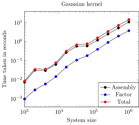
(a) 1D

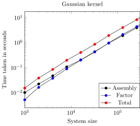
(b) 2D

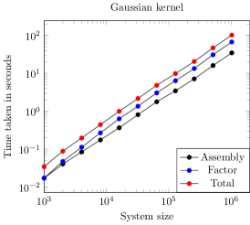
(c) 3D

Fig. 6: Time taken versus system size for Gaussian kernel in different dimensions; The input tolerance was $10^{-12}$ for 1D; $10^{-9}$ for 2D; $10^{-6}$ for 3D;

5.2.2 A biharmonic covariance kernel

As in the previous section, a covariance matrices arising in Gaussian processes can be modeled using the biharmonic covariance kernel, where the $i,j$ entry is given as

(63) $$K(i,j)=\sigma^{2}\delta_{ij}+\dfrac{r_{ij}^{2}}{a^{2}}\log\left(\dfrac{r_{ij}}{a}\right),$$

where the parameters $\sigma$ and $a$ are chosen so that the matrix is positive-definite. Figure 7 presents the results for the Biharmonic kernel in different dimensions.

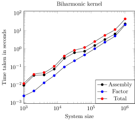
(a) 1D

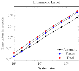
(b) 2D

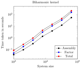
(c) 3D

Fig. 7: Time taken versus system size for biharmonic kernel in different dimensions; The input tolerance was $10^{-12}$ for 1D; $10^{-9}$ for 2D; $10^{-6}$ for 3D;

5.2.3 The Rotne-Prager-Yamakawa tensor

The RPY diffusion tensor is frequently used to model the hydrodynamic interactions in simulations of Brownian dynamics. The RPY tensor is defined as

(64) $$D_{ij}=\begin{cases}\dfrac{k_{B}T}{6\pi\eta a}\left[\left(1-\dfrac{9}{32}\dfrac{r_{ij}}{a}\right)\mathbf{I}+\dfrac{3}{32a}\dfrac{\mathbf{r}_{ij}\otimes\mathbf{r}_{ij}}{r_{ij}}\right]&r<2a,\\ \dfrac{k_{B}T}{8\pi\eta r_{ij}}\left[\mathbf{I}+\dfrac{\mathbf{r}_{ij}\otimes\mathbf{r}_{ij}}{r_{ij}^{2}}+\dfrac{2a^{2}}{3r_{ij}^{2}}\left(\mathbf{I}-3\dfrac{\mathbf{r}_{ij}\otimes\mathbf{r}_{ij}}{r_{ij}^{2}}\right)\right]&r\geq 2a,\end{cases}$$

where $k_{B}$ is the Boltzmann constant, $T$ is the absolute temperature, $\eta$ is the viscosity of the fluid $a$ is the hydrodynamic radius of the particles, $r_{ij}$ is the distance between the $i^{th}$ and $j^{th}$ particle and $\mathbf{r}_{ij}$ is the vector connecting the $i^{th}$ and $j^{th}$ particles. The tensor is obtained as an approximation to the Stokes flow around two spheres by neglecting the hydrodynamic rotation-rotation and rotation-translation coupling. The resulting matrix is often referred to as the mobility matrix. It has been shown in [44] that this tensor is positive-definite for all particle configurations. Fast symmetric factorizations of the RPY tensor are crucial in Brownian dynamics simulations. Geyer and Winter [16] discuss an $\mathcal{O}(n^{2})$ algorithm for approximating the square-root of the RPY tensor. Jiang et al. [26] discuss an approximate algorithm, which relies on a Chebyshev spectral approximation of the matrix square-root coupled with a FMM. Their method scales as $\mathcal{O}(\sqrt{\kappa}n)$, where $\kappa$ is the condition number of the RPY tensor. Our algorithm scales as $\mathcal{O}(n\log^{2}n)$ if the particles are located along a line, $\mathcal{O}(n^{2})$ if the particles are distributed on a surface, and as $\mathcal{O}(n^{7/3})$, if the particles are distributed in a three-dimensional volume.

Remark 14.

Note that since the RPY tensor is singular, on $2$D and $3$D manifolds the ranks of the off-diagonal blocks would grow as $\mathcal{O}(n^{1/2})$ and $\mathcal{O}(n^{2/3})$, respectively. Since the computational cost of the symmetric factorization scales as $\mathcal{O}(p^{2}n)$, the computational cost for the symmetric factorization to scale as $\mathcal{O}(n^{2})$ and $\mathcal{O}(n^{7/3})$ on $2$D and $3$D manifolds, respectively. The numerical benchmarks, plotted in Figure 8, also validate this scaling of our algorithm in all three configurations.

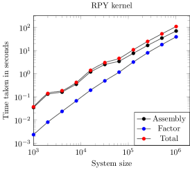
(a) 1D

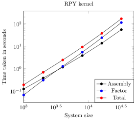
(b) 2D

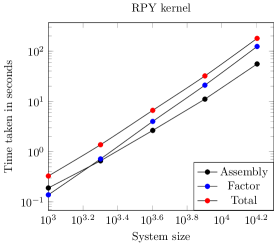
(c) 3D

Fig. 8: Time taken versus system size for the RPY tensor in different dimensions; The input tolerance was $10^{-12}$ for 1D; $10^{-9}$ for 2D; $10^{-6}$ for 3D;

5.2.4 The Matérn Kernel

The Matérn covariance function is frequently used in spatial statistics, geostatistics, Gaussian process regression in machine learning, etc. The covariance function is given by

(65) $$C_{\nu}(r) =\sigma^{2}\dfrac{2^{1-\nu}}{\Gamma(\nu)}\left(\dfrac{r\sqrt{2\nu}}{\rho}\right)^{\nu}K_{\nu}\left(\dfrac{r\sqrt{2\nu}}{\rho}\right)$$

where $K_{\nu}$ is the modified Bessel function of the second kind, $\rho$, $\nu$ are non-negative parameters. When $\nu$ is a half integer, i.e., $\nu=p+1/2$, then Equation (65) simplifies to

(66) $$C_{p+1/2}(r) =\sigma^{2}\exp\left(-\dfrac{r\sqrt{2\nu}}{\rho}\right)\dfrac{\Gamma(p+1)}{\Gamma(2p+1)}\displaystyle\sum_{i=0}^{p}\dfrac{(p+i)!}{i!(p-i)!}\left(\dfrac{r\sqrt{8\nu}}{\rho}\right)^{p-i}$$

The expressions for the first few Matérn kernels are displayed in Table 3. The scaling of the time taken as system size for the first two Matérn kernels are plotted in Figure 9 and 10.

Table 3: Matérn kernel for first few values of $p$

$p=0$	$\sigma^{2}\exp\left(-\dfrac{r}{\rho}\right)$
$p=1$	$\sigma^{2}\left(1+\dfrac{r\sqrt{3}}{\rho}\right)\exp\left(-\dfrac{r\sqrt{3}}{\rho}\right)$
$p=1$	$\sigma^{2}\left(1+\dfrac{r\sqrt{5}}{\rho}+\dfrac{5r^{2}}{3\rho^{2}}\right)\exp\left(-\dfrac{r\sqrt{5}}{\rho}\right)$

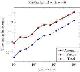
(a) 1D

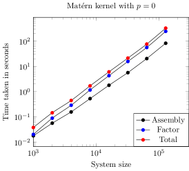
(b) 2D

(c) 3D

Fig. 9: Time taken versus system size for the Matérn kernel with $p=0$ in different dimensions; The input tolerance was $10^{-12}$ for 1D; $10^{-9}$ for 2D; $10^{-6}$ for 3D;

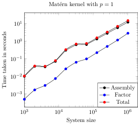
(a) 1D

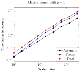
(b) 2D

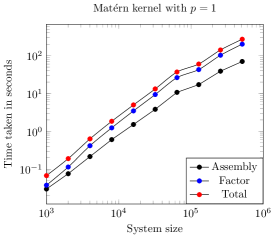
(c) 3D

Fig. 10: Time taken versus system size for the Matérn kernel with $p=1$ in different dimensions; The input tolerance was $10^{-12}$ for 1D; $10^{-9}$ for 2D; $10^{-6}$ for 3D;

6 Conclusion

The article discusses a fast symmetric factorization for a class of symmetric positive-definite hierarchically structured matrices. Our symmetric factorization algorithm is based on two ingredients: a novel formula for the symmetric factorization of a low-rank update to the identity, and a recursive divide-and-conquer strategy compatible with hierarchically structured matrices.

In the case where the hierarchical structure present is that of Hierarchically Off-Diagonal Low-Rank matrices, the algorithm scales as $\mathcal{O}(n\log^{2}n)$. The numerical benchmarks for dense covariance matrix examples validate the scaling. Furthermore, we also applied the algorithm to the mobility matrix encountered in Brownian-hydrodynamics, elements of which are computed from the Rotne-Prager-Yamakawa tensor. In this case, since the ranks of off-diagonal blocks scale as $\mathcal{O}(n^{2/3})$, when the particles are on a three-dimensional manifold, the algorithm scales as $\mathcal{O}(n^{7/3})$. Obtaining an $\mathcal{O}(n)$ symmetric factorization for the mobility matrix is a subject of ongoing research within our group.

It is also worth noting that with nested low-rank basis of the off-diagonal blocks, i.e., if the HODLR matrices are assumed to have a Hierarchical Semi-Separable structure (HSS) instead, then the computational cost of the algorithm would scale as $\mathcal{O}(p^{2}n)$. Extensions to this case is relatively straightforward.

References

- [1] Alkiviadis G Akritas, Evgenia K Akritas, and Genadii I Malaschonok. Various proofs of Sylvester’s (determinant) identity. Mathematics and Computers in Simulation, 42(4):585–593, 1996.
- [2] Sivaram Ambikasaran. Fast Algorithms for Dense Numerical Linear Algebra. PhD thesis, Stanford University, August 2013.
- [3] Sivaram Ambikasaran and Eric Darve. An fast direct solver for partial hierarchically semi-separable matrices. Journal of Scientific Computing, pages 1–25, 2013.
- [4] Sivaram Ambikasaran and Eric Darve. The inverse fast multipole method. arXiv preprint arXiv:1407.1572, 2014.
- [5] Sivaram Ambikasaran, Daniel Foreman-Mackey, Leslie Greengard, David W Hogg, and Michael O’Neil. Fast direct methods for Gaussian processes and the analysis of NASA Kepler mission data. arXiv preprint arXiv:1403.6015, 2014.
- [6] Sivaram Ambikasaran, Judith Yue Li, Peter K Kitanidis, and Eric Darve. Large-scale stochastic linear inversion using hierarchical matrices. Computational Geosciences, 17(6):913–927, 2013.
- [7] Sivaram Ambikasaran, Arvind Krishna Saibaba, Eric F Darve, and Peter K Kitanidis. Fast algorithms for Bayesian inversion. In Computational Challenges in the Geosciences, pages 101–142. Springer, 2013.
- [8] Amirhossein Aminfar, Sivaram Ambikasaran, and Eric Darve. A fast block low-rank dense solver with applications to finite-element matrices. arXiv preprint arXiv:1403.5337, 2014.
- [9] Åke Björck and Sven Hammarling. A Schur method for the square root of a matrix. Linear algebra and its applications, 52:127–140, 1983.
- [10] Steffen Börm, Lars Grasedyck, and Wolfgang Hackbusch. Hierarchical matrices. Lecture notes, 21, 2003.
- [11] Shivkumar Chandrasekaran, Patrick Dewilde, Ming Gu, William Lyons, and Timothy Pals. A fast solver for HSS representations via sparse matrices. SIAM Journal on Matrix Analysis and Applications, 29(1):67–81, 2006.
- [12] Shivkumar Chandrasekaran, Ming Gu, and Timothy Pals. A fast ULV decomposition solver for hierarchically semiseparable representations. SIAM Journal on Matrix Analysis and Applications, 28(3):603–622, 2006.
- [13] Jie Chen. Data structure and algorithms for recursively low-rank compressed matrices. Argonne National Laboratory, 2014.
- [14] Andrzej Cichocki, Rafal Zdunek, Anh Huy Phan, and Shunichi Amari. Nonnegative matrix and tensor factorizations: applications to exploratory multi-way data analysis and blind source separation. John Wiley & Sons, 2009.
- [15] Matthieu Geist and Olivier Pietquin. Statistically linearized recursive least squares. In Machine Learning for Signal Processing (MLSP), 2010 IEEE International Workshop on, pages 272–276. IEEE, 2010.
- [16] Tihamér Geyer and Uwe Winter. An approximation for hydrodynamic interactions in brownian dynamics simulations. The Journal of chemical physics, 130(11):114905, 2009.
- [17] Philip E Gill, Gene H Golub, Walter Murray, and Michael A Saunders. Methods for modifying matrix factorizations. Mathematics of Computation, 28(126):505–535, 1974.
- [18] Lars Grasedyck and Wolfgang Hackbusch. Construction and arithmetics of -matrices. Computing, 70(4):295–334, 2003.
- [19] Leslie Greengard and Vladimir Rokhlin. A fast algorithm for particle simulations. Journal of Computational Physics, 73(2):325–348, 1987.
- [20] Wolfgang Hackbusch. A sparse matrix arithmetic based on -matrices. Part I: Introduction to -matrices. Computing, 62(2):89–108, 1999.
- [21] Wolfgang Hackbusch and Steffen Börm. Data-sparse approximation by adaptive -matrices. Computing, 69(1):1–35, 2002.
- [22] Wolfgang Hackbusch, Boris Khoromskij, and Stefan A Sauter. On -matrices. In Hans-Joachim Bungartz, RonaldH.W. Hoppe, and Christoph Zenger, editors, Lectures on Applied Mathematics, pages 9–29. Springer Berlin Heidelberg, 2000.
- [23] Wolfgang Hackbusch and Boris N Khoromskij. A sparse -matrix arithmetic. Computing, 64(1):21–47, 2000.
- [24] Wolfgang Hackbusch, Boris N Khoromskij, and Ronald Kriemann. Hierarchical matrices based on a weak admissibility criterion. Computing, 73(3):207–243, 2004.
- [25] Nicholas J Higham. Newton’s method for the matrix square root. Mathematics of Computation, 46(174):537–549, 1986.
- [26] Shidong Jiang, Zhi Liang, and Jingfang Huang. A fast algorithm for brownian dynamics simulation with hydrodynamic interactions. Mathematics of Computation, 82(283):1631–1645, 2013.
- [27] Jun Lai, Sivaram Ambikasaran, and Leslie F Greengard. A fast direct solver for high frequency scattering from a large cavity in two dimensions. arXiv preprint arXiv:1404.3451, 2014.
- [28] Judith Yue Li, Sivaram Ambikasaran, Eric F Darve, and Peter K Kitanidis. A kalman filter powered by h2-matrices for quasi-continuous data assimilation problems. Water Resources Research, 2014.
- [29] William Lyons. Fast algorithms with applications to PDEs. PhD thesis, University of California Santa Barbara, 2005.
- [30] Jan Mandel. Efficient implementation of the ensemble Kalman filter. University of Colorado at Denver and Health Sciences Center, Center for Computational Mathematics, 2006.
- [31] Per-Gunnar Martinsson. A fast randomized algorithm for computing a hierarchically semiseparable representation of a matrix. SIAM Journal on Matrix Analysis and Applications, 32(4):1251–1274, 2011.
- [32] Georges Matheron. Principles of geostatistics. Economic geology, 58(8):1246–1266, 1963.
- [33] V Paul Pauca, Jon Piper, and Robert J Plemmons. Nonnegative matrix factorization for spectral data analysis. Linear algebra and its applications, 416(1):29–47, 2006.
- [34] Sergej Rjasanow. Adaptive cross approximation of dense matrices. IABEM 2002, International Association for Boundary Element Methods, 2002.
- [35] Arvind Krishna Saibaba, Sivaram Ambikasaran, Judith Yue Li, Peter K Kitanidis, and Eric F Darve. Application of hierarchical matrices to linear inverse problems in geostatistics. Oil and Gas Science and Technology-Revue de l’IFP-Institut Francais du Petrole, 67(5):857, 2012.
- [36] Matthias Seeger et al. Low rank updates for the Cholesky decomposition. University of California at Berkeley, Tech. Rep, 2007.
- [37] Harold P Starr Jr. On the numerical solution of one-dimensional integral and differential equations. Technical report, DTIC Document, 1991.
- [38] Gilbert W Stewart. Matrix Algorithms: Volume 1, Basic Decompositions, volume 1. Cambridge University Press, 1998.
- [39] Terence Tao. Topics in random matrix theory, Volume 132. American Mathematical Soc., 2012.
- [40] Hans Wackernagel. Multivariate geostatistics. Springer, 2003.
- [41] Dingding Wang, Tao Li, Shenghuo Zhu, and Chris Ding. Multi-document summarization via sentence-level semantic analysis and symmetric matrix factorization. In Proceedings of the 31st annual international ACM SIGIR conference on Research and development in information retrieval, pages 307–314. ACM, 2008.
- [42] Jianlin Xia, Shivkumar Chandrasekaran, Ming Gu, and Xiaoye S Li. Superfast multifrontal method for large structured linear systems of equations. SIAM Journal on Matrix Analysis and Applications, 31(3):1382–1411, 2009.
- [43] Jianlin Xia and Ming Gu. Robust approximate Cholesky factorization of rank-structured symmetric positive definite matrices. SIAM Journal on Matrix Analysis and Applications, 31(5):2899–2920, 2010.
- [44] Hiromi Yamakawa. Transport properties of polymer chains in dilute solution: hydrodynamic interaction. The Journal of Chemical Physics, 53(1):436–443, 2003.
- [45] Lexing Ying. Fast algorithms for boundary integral equations. In Multiscale Modeling and Simulation in Science, pages 139–193. Springer, 2009.
- [46] EL Yip. A note on the stability of solving a rank- modification of a linear system by the Sherman-Morrison-Woodbury formula. SIAM Journal on Scientific and Statistical Computing, 7(2):507–513, 1986.
- [47] Kezhong Zhao, Marinos N Vouvakis, and J-F Lee. The adaptive cross approximation algorithm for accelerated method of moments computations of emc problems. Electromagnetic Compatibility, IEEE Transactions on, 47(4):763–773, 2005.