Cellular buckling in stiffened plates

Abstract

An analytical model based on variational principles for a thin-walled stiffened plate subjected to axial compression is presented. A system of nonlinear differential and integral equations is derived and solved using numerical continuation. The results show that the system is susceptible to highly unstable local–global mode interaction after an initial instability is triggered. Moreover, snap-backs in the response showing sequential destabilization and restabilization, known as cellular buckling or snaking, arise. The analytical model is compared to static finite element models for joint conditions between the stiffener and the main plate that have significant rotational restraint. However, it is known from previous studies that the behaviour, where the same joint is insignificantly restrained rotationally, is captured better by an analytical approach than by standard finite element methods; the latter being unable to capture cellular buckling behaviour even though the phenomenon is clearly observed in laboratory experiments.

1 Introduction

The buckling of thin plates that are stiffened in the longitudinal direction represents a structural instability problem of enormous practical significance [Murray, 1973, Ronalds, 1989, Sheikh et al., 2002, Ghavami & Khedmati, 2006]. Since they are primarily used in structures where mass efficiency is a key design consideration, stiffened plates tend to comprise slender plate elements that are vulnerable to a variety of different elastic instability phenomena. In the current work, the classic problem of a panel comprising a uniform flat plate stiffened by several evenly spaced blade-type longitudinal stiffeners under axial compression, made from a linear elastic material, is studied using an analytical approach. Under this type of loading, wide panels with many stiffeners can be divided into several struts, each with a single stiffener. These individual struts are primarily susceptible to a global (or overall) mode of instability namely Euler buckling, where flexure about the axis parallel to the main plate occurs once the theoretical global buckling load is reached. However, when the individual plate elements of the strut cross-section, namely the main plate and the stiffener, are relatively thin or slender, elastic local buckling of these may also occur; if this happens in combination with the global instability, the resulting behaviour is usually far more unstable than when the modes are triggered individually [Budiansky, 1976].

In the current work, the development of a variational model is presented that accounts for the interaction between the global Euler buckling mode and the local buckling mode of the stiffener, such that the perfect and imperfect elastic post-buckling response can be evaluated. A system of nonlinear ordinary differential equations subject to integral constraints is derived and solved using the numerical continuation package Auto-07p [Doedel & Oldeman, 2011]. It is indeed found that the system is highly unstable when interactive buckling is triggered; snap-backs in the response show a sequence of destabilization and restabilization derived from the mode interaction and the stretching of the plate surface during local buckling respectively. This results in a progressive spreading of the initial localized buckling mode. This latter type of response has become known in the literature as cellular buckling [Hunt et al., 2000] or snaking [Burke & Knobloch, 2007] and it is shown to appear naturally in the current numerical results. The effect is particularly strong where the rotational restraint provided at the joint between the main plate and the stiffener is negligible. As far as the authors are aware, this is the first time this phenomenon has been found analytically in stiffened plates undergoing global and local buckling simultaneously. Similar behaviour has been discovered in various other mechanical systems such as in the post-buckling of cylindrical shells [Hunt et al., 2003], the sequential folding of geological layers [Wadee & Edmunds, 2005], the buckling of thin-walled I-section beams [Wadee & Gardner, 2012] and columns [Wadee & Bai, 2013].

In previous work, cellular buckling has been captured in physical tests for some closely related structures that suffer from local–global mode interaction [Becque & Rasmussen, 2009, Wadee & Gardner, 2012]; it is revealed by the buckling elements exhibiting a progressively varying deformation wavelength. However, by increasing the rotational stiffness of the aforementioned joint, the snap-backs are moderated and the equilibrium path shows an initially smoother response with the snap-backs appearing later in the interactive buckling process. For these cases, the results from a purely numerical model, formulated within the commercial finite element (FE) package Abaqus [Abaqus, 2011], are used to validate the analytical model and exhibit very good correlation, leading to the conclusion that the physics of the system is captured accurately by the analytical model.

2 Analytical Model

2.1 Modal Description

Consider a thin-walled simply-supported plated panel that has uniformly spaced stiffeners above and below the main plate, as shown in Figure 1

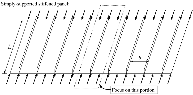
Figure 1: (a) Axially compressed simply-supported stiffened panel of length $L$. (b) Elevation and (c) cross-section of the representative panel portion compressed by a force $P$ applied to the centroid. (d–e) Sway and tilt components respectively of the major axis global buckling mode.

with the associated coordinate system. The panel length is $L$ and the spacing between the stiffeners is $b$. It is made from a linear elastic, homogeneous and isotropic material with Young’s modulus $E$, Poisson’s ratio $\nu$ and shear modulus $G=E/[2(1+\nu)]$. A portion of the panel that is representative of its entirety can be isolated as a strut, shown in Figure 1(b–c), since the transverse bending curvature of the panel during buckling would be relatively small, particularly if $L\ll n_{s}b$, where $n_{s}$ is the number of stiffeners in the panel. The main plate (width $b$ and thickness $t_{p}$) has upper and lower stiffeners (heights $h_{1}$ and $h_{2}$ respectively with equal thickness $t_{s}$) connected to it. The strut is loaded by an axial force $P$ that is applied to the centroid of the cross-section. Presently, however, although the model is formulated for the general case, the numerical results focus on the practically significant case where the stiffeners are only connected to one side of the panel, i.e. where $h_{2}=t_{p}/2$.

Moreover, the geometries are chosen such that global (Euler) buckling about the $x$-axis is the first instability mode encountered by the strut, before any local buckling in the main plate or stiffener occurs. The formulation for global buckling is based on small deflection assumptions, since it is well known that it has an approximately flat (or weakly stable) post-buckling response [Thompson & Hunt, 1973]. The study is primarily concerned with global buckling forcing the stiffener to buckle locally shortly after or even simultaneously. It has been shown in several works [Hunt & Wadee, 1998, Wadee et al., 2010, Wadee & Gardner, 2012, Wadee & Bai, 2013] that shear strains need to be included to model the local–global mode interaction analytically. For thin-walled components, rather than, for instance, soft core materials used in sandwich structures [Wadee et al., 2010], Timoshenko beam theory gives sufficiently accurate results [Wadee & Gardner, 2012]. This can be applied to global flexural buckling within the framework of two degrees of freedom, known as “sway” and “tilt” in the literature [Hunt & Wadee, 1998]. These are associated with functions describing the lateral displacement $W$ and the angle of inclination $\theta$ respectively defining the appropriate kinematics, as shown in Figure 1(c). From linear theory, it can be shown that $W(z)$ and $\theta(z)$ can be represented by the following expressions:

$$W(z)=-q_{s}L\sin\frac{\pi z}{L},\quad\theta(z)=q_{t}\pi\cos\frac{\pi z}{L}.$$ (1)

The quantities $q_{s}$ and $q_{t}$ are the generalized coordinates of the sway and tilt components of global buckling respectively. The corresponding shear strain $\gamma_{yz}$ during bending is given by the following expression:

$$\gamma_{yz}=\frac{\mbox{$\,\mathrm{d}$}W}{\mbox{$\,\mathrm{d}$}z}+\theta=-\left(q_{s}-q_{t}\right)\pi\cos\frac{\pi z}{L}.$$ (2)

Of course, if standard Euler–Bernoulli bending were used then $\gamma_{yz}$ would be zero and $q_{s}$ would be equal to $q_{t}$. The initial global buckling displacement is assumed to put the stiffener into extra compression and it therefore becomes vulnerable to local buckling. The direction of global buckling is crucially important; if the stiffener goes into extra compression and buckles locally it can lead to excessive deflection. This can induce plasticity within the stiffener, leading to the tripping phenomenon that can lead to catastrophic failure of panels [Ronalds, 1989, Butler et al., 2001]; currently, however, linear elasticity is assumed throughout.

The stiffener is taken to be a flat plate (blade-type) and the local kinematics of it require careful consideration. A linear distribution in $y$ for the local in-plane displacement $u(y,z)$ is assumed owing to the application of Timoshenko beam theory. The tips of the stiffeners have free edges but a rotational spring with stiffness $c_{p}$ is included to model the resistance to rotation about the $z$-axis that the joint provides between the stiffeners and the main plate. Hence, if $c_{p}=0$, the stiffeners are effectively pinned with the main plate. In the generic case ($c_{p}>0$), however, the assumed out-of-plane displacement along the width of the stiffener $w(y,z)$ can be approximated by a function that is a summation of trigonometric and polynomial terms. Figure 2

Figure 2: (a) Local out-of-plane displacement $w(y,z)$ and an additional displacement $w_{0}(y,z)$ that represents an initial imperfection in the stiffener geometry; (b) a pinned connection with an additional rotational spring of stiffness $c_{p}$ to model joint fixity; (c) the local in-plane displacement $u(y,z)$. (d) Introduction of the global imperfection functions $W_{0}$ and $\theta_{0}$; for the consideration of the local imperfection, $w_{0}$ would replace $W_{0}$ and apply only to the stiffener.

shows the form of the functions $w$ and $u$ with the algebraic expressions being given thus:

$$u(y,z)=Y(y)u(z),\quad w(y,z)=f(y)w(z),$$ (3)

where $Y(y)=(y+\bar{y})/h_{1}$ and

$$f(y)=B_{0}+B_{1}Y+B_{2}Y^{2}+B_{3}Y^{3}+B_{4}\sin\left(\pi Y\right),$$ (4)

with $B_{0}$, $B_{1}$, $B_{2}$, $B_{3}$ and $B_{4}$ being constants evaluated by solving for the appropriate boundary conditions for the stiffener. The choice of shape for $f$ reflects the possibility of the slope at the junction between the main plate and the stiffener being small in the less compressed zone of the stiffener. For $y=-\bar{y}$, at the junction between stiffener and the main plate, the conditions are:

$$w(\bar{y},z)=0,\quad D\frac{\partial^{2}}{\partial y^{2}}w(\bar{y},z)=c_{p}\frac{\partial}{\partial y}w(\bar{y},z),$$ (5)

and for $y=h_{1}-\bar{y}$, the free-end, the conditions are:

$$D\frac{\partial^{2}}{\partial y^{2}}w(h_{1}-\bar{y},z)=0,\quad D\frac{\partial^{3}}{\partial y^{3}}w(h_{1}-\bar{y},z)=0,$$ (6)

where $\bar{y}$ is the location of the neutral-axis of bending measured from the centre line of the main plate, expressed thus:

$$\bar{y}=\frac{t_{s}\left[h_{1}^{2}-h_{2}^{2}\right]}{2\left[\left(b-t_{s}\right)t_{p}+\left(h_{1}+h_{2}\right)t_{s}\right]}.$$ (7)

By applying the boundary conditions, the function for the deflected shape of the stiffener $w(y,z)$ is found to be:

$$w(y,z)=\left\{Y-S_{4}\frac{\pi^{3}}{6}\left[2Y-3Y^{2}+Y^{3}-\frac{6}{\pi^{3}}\sin\left(\pi Y\right)\right]\right\}w(z),$$ (8)

where:

$$S_{4}=\left\{\pi\left[(D\pi^{2})/(c_{p}h_{1})+\pi^{2}/3-1\right]\right\}^{-1}.$$ (9)

In the current study, both perfect and imperfect panels are considered. A displacement $W_{0}$ corresponding to $W$ and a rotation $\theta_{0}$ corresponding to $\theta$ are introduced; the respective expressions being:

$$W_{0}(z)=-q_{s0}L\sin\frac{\pi z}{L},\quad\theta_{0}=q_{t0}\pi\cos\frac{\pi z}{L},$$ (10)

with $q_{s0}$ and $q_{t0}$ being the amplitudes defining the initial global imperfection. A local imperfection $w_{0}(y,z)=f(y)w_{0}(z)$, see Figure 2(a), is also introduced, the form of which is derived from a first order approximation of a multiple scale perturbation analysis of a strut on a softening foundation [Wadee et al., 1997]:

$$w_{0}(z)=A_{0}\operatorname{sech}\left[\frac{\alpha\left(z-\eta\right)}{L}\right]\cos\left[\frac{\beta\pi\left(z-\eta\right)}{L}\right],$$ (11)

where $z=[0,L]$ and $w_{0}$ is symmetric about $z=\eta$. This form for $w_{0}$ has been shown to be representative for local–global mode interaction problems in the literature [Wadee, 2000]. It enables the study of periodic and localized imperfections, the latter being shown to be relatively more severe for related problems [Wadee, 2002, Wadee & Simões da Silva, 2005].

2.2 Total Potential Energy

The governing equations of equilibrium are derived from variational principles by minimizing the total potential energy $V$ of the system. The total potential energy comprises the contributions of global and local strain energies of bending, $U_{bo}$ and $U_{bl}$ respectively, the strain energy stored in the “membrane” of the stiffener $U_{m}$ arising from axial and shear stresses, and the work done by the external load $P\mathcal{E}$. The effects of the initial imperfections are evaluated by assuming that the imperfect forms, given by the functions $W_{0}$ and $w_{0}$, are stress-relieved. This implies that the elemental moment $M$ and hence the bending energy both drop to zero in the unloaded state, see Figure 2(d). The global bending energy accounts for the main plate and is hence given by:

$$U_{bo}=\frac{1}{2}EI_{p}\int_{0}^{L}\left(\ddot{W}-\ddot{W}_{0}\right)^{2}\mbox{$\,\mathrm{d}$}z=\frac{1}{2}EI_{p}\int_{0}^{L}\left(q_{s}-q_{s0}\right)^{2}\frac{\pi^{4}}{L^{2}}\sin^{2}\frac{\pi z}{L}\mbox{$\,\mathrm{d}$}z,$$ (12)

where dots represent differentiation with respect to $z$ and $I_{p}=(b-t_{s})t_{p}^{3}/12+(b-t_{s})t_{p}\bar{y}^{2}$ is the second moment of area of the main plate about the global $x$-axis. The local bending energy $U_{bl}$, accounting for the stiffener only, is given thus:

$$U_{bl} =\frac{D}{2}\int_{0}^{L}\int_{-\bar{y}}^{h_{1}-\bar{y}}\left\{\left[\frac{\partial^{2}(w-w_{0})}{\partial z^{2}}+\frac{\partial^{2}(w-w_{0})}{\partial y^{2}}\right]^{2}\right.$$ (13)

$$\left.\qquad-2\left(1-\nu\right)\left[\frac{\partial^{2}(w-w_{0})}{\partial z^{2}}\frac{\partial^{2}(w-w_{0})}{\partial y^{2}}-\left(\frac{\partial^{2}(w-w_{0})}{\partial z\partial y}\right)^{2}\right]\right\}\mbox{$\,\mathrm{d}$}y\mbox{$\,\mathrm{d}$}z,$$

$$=\frac{D}{2}\int_{0}^{L}\left[\{f^{2}\}_{y}\left(\ddot{w}-\ddot{w}_{0}\right)^{2}+\bigl{\{}f^{\prime\prime 2}\bigr{\}}_{y}(w-w_{0})^{2}+2\nu\bigl{\{}ff^{\prime\prime}\bigr{\}}_{y}(w-w_{0})(\ddot{w}-\ddot{w_{0}})\right.$$

$$\left.\qquad+2(1-\nu)\bigl{\{}f^{\prime 2}\bigr{\}}_{y}(\dot{w}-\dot{w_{0}})^{2}\right]\mbox{$\,\mathrm{d}$}z,$$

where primes denote differentiation with respect to $y$, $D$ is the plate flexural rigidity given by $Et_{s}^{3}/[12(1-\nu^{2})]$ and:

$$\{F(y)\}_{y}=\int_{-\bar{y}}^{h_{1}-\bar{y}}F(y)\mbox{$\,\mathrm{d}$}y,$$ (14)

where $F$ is an example function. The compressive side of the panel only contributes to the local bending energy once global buckling occurs. The membrane energy $U_{m}$ is derived from considering the direct strains ($\varepsilon$) and shear strains ($\gamma$) in the stiffener. The global buckling distribution for the longitudinal strain $\varepsilon_{z}$ can be obtained from the tilt component of displacement from the global mode, thus:

$$\varepsilon_{z,\mathrm{global}}=y\frac{\mbox{$\mathrm{d}$}}{\mbox{$\mathrm{d}$}z}\left(\theta-\theta_{0}\right)=-y\left(q_{t}-q_{t0}\right)\frac{\pi^{2}}{L}\sin\frac{\pi z}{L}.$$ (15)

The local mode contribution is based on von Kármán plate theory. A purely in-plane compressive strain $\Delta$ is also included. The direct strain for the main plate is given by: $\varepsilon_{zp}=-\Delta$. The combined expressions for the direct strains for the top and bottom stiffeners $\varepsilon_{zt}$ and $\varepsilon_{zb}$ respectively, including local and global buckling are:

$$\varepsilon_{zt} =-y\left(q_{t}-q_{t0}\right)\frac{\pi^{2}}{L}\sin\frac{\pi z}{L}-\Delta+\frac{\partial u}{\partial z}+\frac{1}{2}\left(\frac{\partial w}{\partial z}\right)^{2}-\frac{1}{2}\left(\frac{\partial w_{0}}{\partial z}\right)^{2},$$ (16)

$$=-y\left(q_{t}-q_{t0}\right)\frac{\pi^{2}}{L}\sin\frac{\pi z}{L}-\Delta+\left(\frac{y+\bar{y}}{h_{1}}\right)\dot{u}+\frac{1}{2}\{f^{2}\}_{y}\left(\dot{w}^{2}-\dot{w}_{0}^{2}\right),$$

$$\varepsilon_{zb}=-y\left(q_{t}-q_{t0}\right)\frac{\pi^{2}}{L}\sin\frac{\pi z}{L}-\Delta.$$ (17)

The complete expression for the membrane strain energy $U_{m}$ is given by:

$$U_{m} =U_{d}+U_{s}$$ (18)

$$=\frac{1}{2}\int_{0}^{L}\int_{-t_{s}/2}^{t_{s}/2}\left[\int_{-\bar{y}}^{h_{1}-\bar{y}}\left(E\varepsilon_{zt}^{2}+G\gamma_{yzt}^{2}\right)\mbox{$\mathrm{d}$}y+\int_{-(h_{2}+\bar{y})}^{-\bar{y}}\left(E\varepsilon_{zb}^{2}+G\gamma_{yzb}^{2}\right)\mbox{$\mathrm{d}$}y\right]\mbox{$\mathrm{d}$}x\mbox{$\,\mathrm{d}$}z,$$

where $U_{d}$ is the contribution from direct strains, which is given by the terms multiplied by the Young’s modulus $E$; whereas $U_{s}$, the contribution arising from the shear strains, is given by the terms multiplied by the shear modulus $G$. The transverse component of the strain $\varepsilon_{y}$ is neglected since it has been shown that it has no effect on the post-buckling stiffness of a long plate with three simply-supported edges and one free edge [Koiter & Pignataro, 1976]. The total direct strain energy $U_{d}$ is therefore:

$$U_{d}=\frac{1}{2}E t_{s}\int_{0}^{L}\biggl{\{}\frac{1}{3}\left[\left(h_{1}-\bar{y}\right)^{3}+\left(h_{2}+\bar{y}\right)^{3}\right]\left(q_{t}-q_{t0}\right)^{2}\frac{\pi^{4}}{L^{2}}\sin^{2}\frac{\pi z}{L}$$ (19)

$$+\Delta^{2}\left(h_{1}+h_{2}\right)+\left[\left(h_{1}-\bar{y}\right)^{2}-\left(h_{2}+\bar{y}\right)^{2}\right]\Delta\left(q_{t}-q_{t0}\right)\frac{\pi^{2}}{L}\sin\frac{\pi z}{L}$$

$$+h_{1}\left[\frac{1}{3}{\dot{u}}^{2}+\frac{1}{4h_{1}}\{f^{4}\}_{y}\left(\dot{w}^{2}-\dot{w}_{0}^{2}\right)^{2}+\biggl{\{}\frac{Yf^{2}}{h_{1}}\biggr{\}}_{y}\dot{u}\left(\dot{w}^{2}-\dot{w}_{0}^{2}\right)\right]$$

$$-\left(q_{t}-q_{t0}\right)\frac{h_{1}\pi^{2}}{L}\sin\frac{\pi z}{L}\left[\left(\frac{2}{3}h_{1}-\bar{y}\right)\dot{u}+\frac{1}{h_{1}}\{yf^{2}\}_{y}\left(\dot{w}^{2}-\dot{w}_{0}^{2}\right)\right]$$

$$-h_{1}\Delta\left[\dot{u}+\frac{1}{h_{1}}\{f^{2}\}_{y}\left(\dot{w}^{2}-\dot{w}_{0}^{2}\right)\right]+\left(\frac{t_{p}}{t_{s}}\right)(b-t_{s})\Delta^{2}\biggr{\}}\mbox{$\,\mathrm{d}$}z.$$

The shear strain energy $U_{s}$ requires the shear strain $\gamma_{yz}$, which is also modelled separately for the compression and the tension side of the stiffeners. The general expression for the shear strain $\gamma_{yzi}$ in the stiffeners is thus:

$$\gamma_{yzi}=\frac{\mbox{$\mathrm{d}$}}{\mbox{$\mathrm{d}$}z}\left(W-W_{0}\right)+\left(\theta-\theta_{0}\right)+\frac{\partial u}{\partial y}+\frac{\partial w}{\partial z}\frac{\partial w}{\partial y}-\frac{\partial w_{0}}{\partial z}\frac{\partial w_{0}}{\partial y},$$ (20)

and the expressions for the top and bottom stiffeners are given respectively:

$$\gamma_{yzt} =-\left[\left(q_{s}-q_{s0}\right)-\left(q_{t}-q_{t0}\right)\right]\pi\cos\frac{\pi z}{L}+\frac{u}{h_{1}}+\bigl{\{}ff^{\prime}\bigr{\}}_{y}(w\dot{w}-w_{0}\dot{w_{0}}),$$ (21)

$$\gamma_{yzb} =-\left[\left(q_{s}-q_{s0}\right)-\left(q_{t}-q_{t0}\right)\right]\pi\cos\frac{\pi z}{L},$$

hence, the expression for $U_{s}$ is:

$$U_{s}=\frac{1}{2}G t_{s}\int_{0}^{L}\biggl{\{}\left[\left(q_{s}-q_{s0}\right)-\left(q_{t}-q_{t0}\right)\right]^{2}{\pi}^{2}\cos^{2}\frac{\pi z}{L}\left(h_{1}+h_{2}\right)$$ (22)

$$+\frac{1}{h_{1}}\left[u^{2}+h_{1}\bigl{\{}\left(ff^{\prime}\right)^{2}\bigr{\}}_{y}\left(w\dot{w}-w_{0}\dot{w}_{0}\right)^{2}+2\bigl{\{}ff^{\prime}\bigr{\}}_{y}u\left(w\dot{w}-w_{0}\dot{w}_{0}\right)\right]$$

$$-\left[\left(q_{s}-q_{s0}\right)-\left(q_{t}-q_{t0}\right)\right]\biggl{[}2u+2\bigl{\{}ff^{\prime}\bigr{\}}_{y}(w\dot{w}-w_{0}\dot{w}_{0})\biggr{]}\pi\cos\frac{\pi z}{L}\biggr{\}}\mbox{$\,\mathrm{d}$}z.$$

The strain energy stored in the rotational spring connecting the stiffeners to the main plate is:

$$U_{sp}=\frac{1}{2}c_{p}\int_{0}^{L}\left\{\frac{\partial}{\partial y}\left[w(-\bar{y})-w_{0}(-\bar{y})\right]\right\}^{2}\mbox{$\,\mathrm{d}$}z=\frac{1}{2}c_{p}\int_{0}^{L}[f^{\prime 2}(-\bar{y})](w-w_{0})^{2}\mbox{$\,\mathrm{d}$}z,$$ (23)

where $F(-\bar{y})$ means that the example function $F$ is evaluated at $y=-\bar{y}$. The final component of $V$ is the work done by the axial load $P$, which is given by:

$$P\mathcal{E}=\frac{P}{2}\int_{0}^{L}\left[2\Delta+q_{s}^{2}\pi^{2}\cos^{2}\frac{\pi z}{L}-2\left(\frac{h_{2}+\bar{y}}{h_{1}+h_{2}}\right)\dot{u}\right]\mbox{$\mathrm{d}$}z,$$ (24)

where the total end-displacement $\mathcal{E}$ comprises components from pure squash and sway from global buckling combined with the local buckling of the stiffener respectively. The total potential energy $V$ is given by the summation of all the strain energy terms minus the work done, thus:

$$V=U_{bo}+U_{bl}+U_{m}+U_{sp}-P\mathcal{E}.$$ (25)

2.3 Variational Formulation

The governing equilibrium equations are obtained by performing the calculus of variations on the total potential energy $V$ following a well established procedure that has been detailed in Hunt and Wadee [Hunt & Wadee, 1998]. The integrand of the total potential energy $V$ can be expressed as the Lagrangian ($\mathcal{L}$) of the form:

$$V=\int_{0}^{L}\mathcal{L}\left(\ddot{w},\dot{w},w,\dot{u},u,z\right)\mbox{$\,\mathrm{d}$}z.$$ (26)

The first variation of $V$ is given by:

$$\delta V=\int_{0}^{L}\left[\frac{\partial\mathcal{L}}{\partial\ddot{w}}\delta\ddot{w}+\frac{\partial\mathcal{L}}{\partial\dot{w}}\delta\dot{w}+\frac{\partial\mathcal{L}}{\partial w}\delta w+\frac{\partial\mathcal{L}}{\partial\dot{u}}\delta\dot{u}+\frac{\partial\mathcal{L}}{\partial u}\delta u\right]\mbox{$\,\mathrm{d}$}z,$$ (27)

to determine the equilibrium states, $V$ must be stationary, hence the first variation $\delta V$ must vanish for any small change in $w$ and $u$. Since $\delta\ddot{w}=\mbox{$\mathrm{d}$}(\delta\dot{w})/\mbox{$\,\mathrm{d}$}z$, $\delta\dot{w}=\mbox{$\mathrm{d}$}(\delta w)/\mbox{$\mathrm{d}$}z$ and similarly $\delta\dot{u}=\mbox{$\mathrm{d}$}(\delta u)/\mbox{$\mathrm{d}$}z$, integration by parts allows the development of the Euler–Lagrange equations for $w$ and $u$; these comprise a fourth-order and a second-order nonlinear differential equation for $w$ and $u$ respectively. To facilitate the solution of the equations within the package Auto-07p, the variables are rescaled with respect to the non-dimensional spatial coordinate $\tilde{z}$, defined as $\tilde{z}=2z/L$. Similarly, the non-dimensional out-of-plane and in-plane displacements $\tilde{w}$ and $\tilde{u}$ are defined with the scalings $2w/L$ and $2u/L$ respectively. Note that the scalings exploit symmetry about the midspan and the equations are hence solved for half the strut length; this assumption has been shown to be acceptable for cases where global buckling is critical [Wadee, 2000]. The non-dimensional differential equations are thus:

$$\tilde{\ddddot{w}} -\tilde{\ddddot{w_{0}}}+\frac{L^{2}}{2\{f^{2}\}_{y}}\left[\nu\left\{ff^{\prime\prime}\right\}_{y}-(1-\nu)\left\{f^{\prime 2}\right\}_{y}\right]\left(\tilde{\ddot{w}}-\tilde{\ddot{w}}_{0}\right)+\tilde{k}\left(\tilde{w}-\tilde{w_{0}}\right)$$ (28)

$$-\tilde{D}\left[\frac{\left\{f^{4}\right\}_{y}}{\left\{f^{2}\right\}_{y}}\left(3\tilde{\dot{w}}^{2}\tilde{\ddot{w}}-\tilde{\ddot{w}}{\dot{w}_{0}}^{2}-2\tilde{\ddot{w}}_{0}\tilde{\dot{w}}_{0}\tilde{\dot{w}}\right)+\frac{\left\{2Yf^{2}\right\}_{y}}{\left\{f^{2}\right\}_{y}}\left(\tilde{\ddot{u}}\tilde{\dot{w}}+\tilde{\ddot{w}}\tilde{\dot{u}}\right)\right.$$

$$\left.-2\Delta\tilde{\ddot{w}}-2\left(q_{t}-q_{t0}\right)\frac{\pi^{2}}{L}\frac{\left\{yf^{2}\right\}_{y}}{\left\{f^{2}\right\}_{y}}\left(\sin\frac{\pi\tilde{z}}{2}\tilde{\ddot{w}}+\frac{\pi}{2}\cos\frac{\pi\tilde{z}}{2}\tilde{\dot{w}}\right)\right]$$

$$-\frac{\tilde{G}L^{2}\tilde{w}}{2\left\{f^{2}\right\}_{y}}\biggl{[}\left\{\left(ff^{\prime}\right)^{2}\right\}_{y}\left(\tilde{\dot{w}}^{2}+\tilde{w}\tilde{\ddot{w}}-\tilde{\dot{w}}_{0}^{2}-\tilde{w_{0}}\tilde{\ddot{w}}_{0}\right)+\frac{1}{h}_{1}\left\{ff^{\prime}\right\}_{y}\tilde{\dot{u}}$$

$$+\left[\left(q_{s}-q_{s0}\right)-\left(q_{t}-q_{t0}\right)\right]\frac{\pi^{2}}{L}\left\{ff^{\prime}\right\}_{y}\sin\frac{\pi\tilde{z}}{2}\biggr{]}=0,$$

$$\tilde{\ddot{u}} -\frac{3}{4}\frac{\tilde{G}}{\tilde{D}}\psi\biggl{\{}\psi\left[\tilde{u}+\left\{ff^{\prime}\right\}_{y}\left(\tilde{w}\tilde{\dot{w}}-\tilde{w}_{0}\tilde{\dot{w}}_{0}\right)\right]-2\pi\left[\left(q_{s}-q_{s0}\right)-\left(q_{t}-q_{t0}\right)\right]\cos\frac{\pi\tilde{z}}{2}\biggr{\}}$$ (29)

$$-\left\{\frac{3Y}{h_{1}}f^{2}\right\}_{y}\left(\tilde{\dot{w}}\tilde{\ddot{w}}+\tilde{\dot{w}}_{0}\tilde{\ddot{w}}_{0}\right)+\frac{1}{2}\left(q_{t}-q_{t0}\right)\pi^{3}\left(\psi-\frac{3\bar{y}}{2L}\right)\cos\frac{\pi\tilde{z}}{2}=0,$$

where the rescaled quantities are:

$$\tilde{D}=Et_{s}L^{2}/{8D},\quad\tilde{G}=Gt_{s}L^{2}/{8D},\quad\tilde{k}=\frac{L^{4}}{16\left\{f^{2}\right\}_{y}}\biggl{[}\left\{f^{\prime\prime 2}\right\}_{y}+c_{p}f^{\prime 2}(-\bar{y})/D\biggr{]},$$ (30)

with $\tilde{w}_{0}=2w_{0}/L$, $\psi=L/h_{1}$ and $f^{\prime 2}(-\bar{y})$ is as described previously. Equilibrium also requires the minimization of the total potential energy with respect to the generalized coordinates $\Delta$, $q_{s}$ and $q_{t}$ leading to the three integral equations in nondimensional form:

$$\begin{split}\frac{\partial V}{\partial\Delta}&=\Delta\left[1+\frac{h_{2}}{h_{1}}+\frac{t_{p}(b-t_{s})}{t_{s}}\right]-\frac{P}{Et_{s}h_{1}}+\left(q_{t}-q_{t0}\right)\frac{\pi}{h_{1}L}\left[\left(h_{1}-\bar{y}\right)^{2}-\left(h_{2}+\bar{y}\right)^{2}\right]\\ &-\frac{1}{4}\int_{0}^{2}\left[\tilde{\dot{u}}+\frac{1}{h_{1}}\left\{f^{2}\right\}_{y}\left(\tilde{\dot{w}}^{2}-\dot{w}_{0}^{2}\right)\right]\mbox{$\mathrm{d}$}\tilde{z}=0,\end{split}$$ (31)

$$\begin{split}\frac{\partial V}{\partial q_{s}}&=\pi^{2}\left(q_{s}-q_{s0}\right)+\tilde{s}\left[\left(q_{s}-q_{s0}\right)-\left(q_{t}-q_{t0}\right)\right]-\frac{PL^{2}}{EI_{p}}q_{s}\\ &\quad-\frac{\tilde{s}\tilde{\phi}}{2\pi}\int_{0}^{2}\cos\frac{\pi\tilde{z}}{2}\left[\tilde{u}+\left\{ff^{\prime}\right\}_{y}\left(\tilde{w}\tilde{\dot{w}}-\tilde{w}_{0}\tilde{\dot{w}}_{0}\right)\right]\mbox{$\mathrm{d}$}\tilde{z}=0,\end{split}$$ (32)

$$\begin{split}\frac{\partial V}{\partial q_{t}}&=\pi^{2}\left(q_{t}-q_{t0}\right)+\tilde{\Gamma_{3}}\Delta-\tilde{t}\left[\left(q_{s}-q_{s0}\right)-\left(q_{t}-q_{t0}\right)\right]-\frac{1}{2}\int_{0}^{2}\biggl{\{}\sin\frac{\pi\tilde{z}}{2}\left[\tilde{\Gamma_{1}}\tilde{\dot{u}}\right.\\ &\quad\left.+\tilde{\Gamma_{2}}\left(\tilde{\dot{w}}^{2}-\tilde{\dot{w}}_{0}^{2}\right)\right]-\frac{\tilde{t}\tilde{\phi}}{\pi}\cos\frac{\pi\tilde{z}}{L}\left[\tilde{u}+\left\{ff^{\prime}\right\}_{y}\left(\tilde{w}\tilde{\dot{w}}-\tilde{w_{0}}\tilde{\dot{w}}_{0}\right)\right]\biggr{\}}\mbox{$\mathrm{d}$}\tilde{z}=0,\end{split}$$ (33)

where the rescaled quantities are:

$$\tilde{\Gamma_{1}} =\frac{Lh_{1}\left(2h_{1}-3\bar{y}\right)}{\left(h_{1}-\bar{y}\right)^{3}+\left(h_{2}+\bar{y}\right)^{3}},\quad\tilde{\Gamma_{2}}=\frac{3L\left\{yf^{2}\right\}_{y}}{\left(h_{1}-\bar{y}\right)^{3}+\left(h_{2}+\bar{y}\right)^{3}},$$ (34)

$$\tilde{\Gamma_{3}} =\frac{6L\left[\left(h_{1}-\bar{y}\right)^{2}-\left(h_{2}+\bar{y}\right)^{2}\right]}{\pi\left[\left(h_{1}-\bar{y}\right)^{3}+\left(h_{2}+\bar{y}\right)^{3}\right]},\quad\tilde{\phi}=\frac{L}{h_{1}+h_{2}},$$

$$\tilde{s} =\frac{Gt_{s}(h_{1}+h_{2})L^{2}}{EI_{p}},\quad\tilde{t}=\frac{3GL^{2}(h_{1}+h_{2})}{E\left[\left(h_{1}-\bar{y}\right)^{3}+\left(h_{2}+\bar{y}\right)^{3}\right]}.$$

Since the strut is an integral member, Equations (32)–(33) provide a relationship linking $q_{s}$ and $q_{t}$ before any interactive buckling occurs, i.e. when $w=u=0$. This link is assumed to hold also between $q_{s0}$ and $q_{t0}$, which acts as a simplification by reducing the number of global imperfection amplitude parameters to one; this relationship is given by:

$$q_{s0}=\left(1+\pi^{2}/\tilde{t}\right)q_{t0}.$$ (35)

The boundary conditions for $\tilde{w}$ and $\tilde{u}$ and their derivatives are for simply-supported conditions at $\tilde{z}=0$ and for symmetry conditions at $\tilde{z}=1$:

$$\tilde{w}(0)=\tilde{\ddot{w}}(0)=\tilde{\dot{w}}(1)=\tilde{\dddot{w}}(1)=\tilde{u}(1)=0,$$ (36)

with a further condition from matching the in-plane strain:

$$\frac{1}{3}\tilde{\dot{u}}(0)+\frac{1}{2}\left\{\frac{Y}{h_{1}}f^{2}\right\}_{y}\left[\tilde{\dot{w}}^{2}(0)-\dot{w}_{0}^{2}(0)\right]-\frac{1}{2}\Delta+\frac{P}{Et_{s}h_{1}}\left(\frac{h_{2}+\bar{y}}{h_{1}+h_{2}}\right)=0.$$ (37)

It is worth noting that the terms in braces in Equations (28)–(37) are integrated with respect to the original definition of $y$.

Linear eigenvalue analysis for the perfect strut ($q_{s0}=q_{t0}=A_{0}=0$) is conducted to determine the critical load for global buckling $P_{o}^{\mathrm{C}}$. By considering that the Hessian matrix $\mathbf{V}_{ij}$, thus:

$$\mathbf{V}_{ij}=\left[\begin{array}[]{cc}\frac{\partial^{2}V}{\partial q_{s}^{2}}&\frac{\partial^{2}V}{\partial q_{s}\partial q_{t}}\\ \frac{\partial^{2}V}{\partial q_{t}\partial q_{s}}&\frac{\partial^{2}V}{\partial q_{t}^{2}}\end{array}\right]$$ (38)

at the critical load is singular, in conjunction with the pre-buckling condition $q_{s}=q_{t}=w=u=0$, the critical load for global buckling is obtained:

$$\mbox{$P_{o}^{\mathrm{C}}$}=\frac{\pi^{2}EI_{p}}{L^{2}}\left[1+\frac{\tilde{s}}{\pi^{2}+\tilde{t}}\right].$$ (39)

If the limit $G\rightarrow\infty$ is taken, a primary assumption in Euler–Bernoulli bending theory, $P_{o}^{\mathrm{C}}$ reduces to the expected classical Euler column buckling load.

3 Numerical study

The full system of equilibrium equations are difficult to solve analytically. The continuation and bifurcation software Auto-07p is thus used; it has been shown in previous work [Wadee & Gardner, 2012] to be an ideal tool to solve the equations for this kind of mechanical system. The solver is adept at locating bifurcation points and tracing branching paths as model parameters are varied. To demonstrate this, an example set of geometric and material properties are chosen thus: $L=5000~{}\mbox{$\mathrm{mm}$}$, $b=120~{}\mbox{$\mathrm{mm}$}$, $t_{p}=2.4~{}\mbox{$\mathrm{mm}$}$, $t_{s}=1.2~{}\mbox{$\mathrm{mm}$}$, $h_{1}=38~{}\mbox{$\mathrm{mm}$}$, $h_{2}=t_{p}/2$, $E=210~{}\mathrm{kN/mm^{2}}$, $\nu=0.3$. The global critical load $P_{o}^{\mathrm{C}}$ can be calculated using Equation (39), whereas the local buckling critical stress $\sigma_{l}^{\mathrm{C}}$ can be evaluated using the well-known formula $\sigma_{l}^{\mathrm{C}}=k_{p}D\pi^{2}/(b^{2}t)$, where the coefficient $k_{p}$ depends on plate boundary conditions; limiting values being $k_{p}=0.426$ and $k_{p}=1.247$ for a long stiffener connected to the main plate with one edge free and the edge defining the junction between the stiffener and the main plate being taken to be pinned or fixed respectively. For the panel selected, Table 1

$\sigma_{o}^{\mathrm{C}}~{}(\mathrm{N/mm^{2}})$	$\sigma_{l,s}^{\mathrm{C}}~{}(\mathrm{N/mm^{2}})$	$\sigma_{l,p}^{\mathrm{C}}~{}(\mathrm{N/mm^{2}})$	Critical mode
$4.89$	$80.22$	$373.28$	Global

Table 1: Theoretical values of the global and local critical buckling stresses ($\sigma_{o}^{\mathrm{C}}$ and $\sigma_{l}^{\mathrm{C}}$) respectively; subscripts “$p$” and “$s$” refer to the main plate and the stiffener respectively. The expression for $\sigma_{o}^{\mathrm{C}}=\mbox{$P_{o}^{\mathrm{C}}$}/A$, where $A$ is the cross-sectional area of the strut.

shows that global buckling is critical and that the stiffener could be the next in line to buckle locally since its critical stress is much less than that of the main plate.

3.1 Analytical model results

To solve the governing equations, the principal parameters used in the numerical continuation procedure in Auto-07p were interchangeable although generally $q_{s}$ was varied for computing the equilibrium paths for the distinct buckling modes. However, the load $P$ was used as the principal continuation parameter for computing the interactive buckling paths. The perfect post-buckling path was computed first from $P_{o}^{\mathrm{C}}$ and then a sequence of bifurcation points were detected on the weakly stable post-buckling path; the value of $q_{s}$ closest to the critical bifurcation point ($\mathrm{C}$) was identified as the secondary bifurcation point ($\mathrm{S}$), see Figure 3, and denoted as $q_{s}^{\mathrm{S}}$.

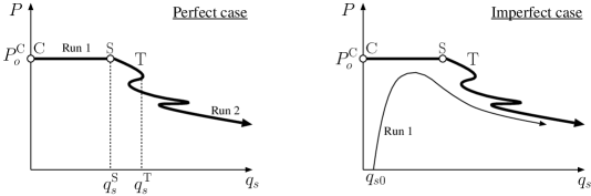
Figure 3: Diagrammatic representation of the sequence for computing the equilibrium paths for the (left) perfect and (right) imperfect cases.

This triggered interactive buckling and a new equilibrium path was computed. Typically this reduced the load $P$ with $w$ and $u$ becoming non-trivial as the interaction advanced. On the interactive buckling path, a progressive sequence of destabilization and restabilization, exhibited as a series of snap-backs in the equilibrium paths was observed – the signature of cellular buckling [Hunt et al., 2000, Wadee & Edmunds, 2005, Wadee & Gardner, 2012, Wadee & Bai, 2013]. In Figure 3, the first such snap-back is labelled as $\mathrm{T}$ with $q_{s}=q_{s}^{\mathrm{T}}$ and the existence of it marks the beginning of the rapid spreading of the buckling profile from being localized to being eventually periodic.

For the example panel being considered, Figure 4

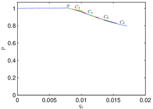
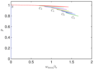
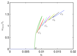
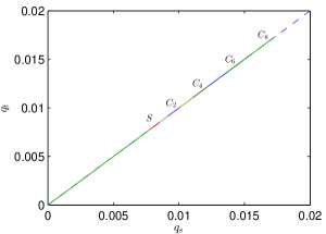
Figure 4: Numerical solutions from the analytical model: equilibrium paths. Normalized force $p$ versus the normalized amplitudes of (a) global buckling $q_{s}$ and (b) local buckling of the stiffener $w_{\mathrm{max}}/t_{s}$. Modal amplitude comparisons: (c) local versus global; (d) sway versus tilt.

shows equilibrium plots of the normalized axial load $p=P/\mbox{$P_{o}^{\mathrm{C}}$}$ versus the normalized buckling amplitudes of (a) the global mode of the strut and (b) the local mode of the stiffener. The graph in (c) shows the relative amplitudes of the global and local buckling modes. Finally, (d) shows the relationship between the sway and tilt amplitudes of global buckling, which are almost equal; indicating that the shear strain from the global mode is small but, importantly, not zero. Figure 5

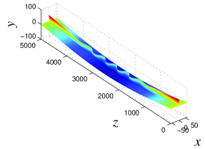
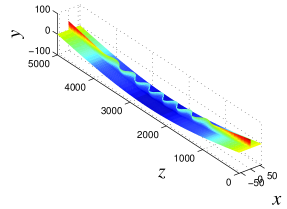
Figure 5: Numerical solutions from the analytical model visualized on 3-dimensional representations of the strut. (a) Secondary bifurcation point $\mathrm{S}~{}(p=1.00)$, (b) cell $C_{4}~{}(p=0.976)$, (c) cell $C_{6}~{}(p=0.926)$ and (d) cell $C_{8}~{}(p=0.865)$. All dimensions are in millimetres, but the local buckling displacements in the stiffener are scaled by a factor of 5 to aid visualization.

shows a selection of 3-dimensional representations of the deflected strut that include the components of global buckling ($q_{s}$ and $q_{t}$) and local buckling ($w$ and $u$) for $\mathrm{S}$ and cells $C_{4}$, $C_{6}$, and $C_{8}$ respectively. Figure 6

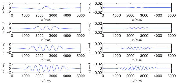
Figure 6: Numerical solutions for the local buckling mode out-of-plane deflection $w$ (left) and in-plane deflection $u$ (right) showing the progressive spreading of the stiffener deflection for cells $C_{2}$, $C_{4}$, $C_{6}$ and $C_{8}$ (top to bottom respectively) of the perfect case from the analytical model.

illustrates the corresponding progression of the numerical solutions for the local buckling functions $w$ and $u$. The results for the example clearly shows cellular buckling with the spiky features in the graphs in Figure 4(a–c). Moreover, the buckling patterns, as seen in Figure 5, clearly show an initially localized buckle gradually spreading outwards from the panel midspan with more peaks and troughs.

In the literature [Hunt et al., 2000, Wadee & Edmunds, 2005] the Maxwell load ($P^{\mathrm{M}}$) is calculated for snaking problems, which represents a realistic lower bound strength for the system. Presently, however, it is more complex to determine such a quantity because the system axial load $P$ does not oscillate about a fixed load $P^{\mathrm{M}}$ as the deformation increases. This is primarily owing to the fact that, unlike systems that exhibit cellular buckling, such as cylindrical shells and confined layered structures [Hunt et al., 2000], there are two effective loading sources as the mode interaction takes hold: the axial load $P$, which generally decreases and the sinusoidally varying (in $z$) tilt generalized coordinate $q_{t}$, which represents the axial component of the global buckling mode that generally increases. The notion of determining the “body force”, discussed in Hunt and Wadee [Hunt & Wadee, 1998], could be used as way to calculate the Maxwell load, but this has been left for future work.

Hitherto, the results have been presented for the case where the joint between the main plate and the stiffener is pinned ($c_{p}=0$). Figure 7

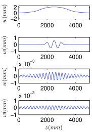
(a) $p=0.99$

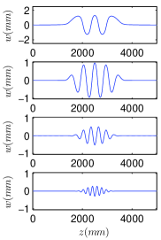
(b) $p=0.96$

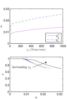
Figure 7: (a–b) Numerical solutions from the analytical model for the local out-of-plane deflection $w$ in the initial interactive buckling stage, where cases for $c_{p}=0,10,100,1000~{}\mathrm{Nmm/mm}$ are shown from top to bottom respectively. (c) Curves showing the distribution of $q_{s}^{\mathrm{S}}$ and $q_{s}^{\mathrm{T}}$, and the load $p$ versus $q_{s}$ for the increasing values of $c_{p}$ given in (a–b).

shows how the introduction of the joint stiffness affects the response. First of all, the value of $\sigma_{l,s}^{\mathrm{C}}$ is increased since rotation at the joint is more restrained. This, in turn, increases the value of $q_{s}^{\mathrm{S}}$ and $q_{s}^{\mathrm{T}}$ at different rates. It can be seen that as $c_{p}$ is increased the initial interactive mode that emerges from the secondary bifurcation $\mathrm{S}$ is more localized with a smaller wavelength (Figure 7) and resembles the more advanced cells shown in Figure 6 directly. Moreover, it is demonstrated that the snap-backs occur later in the interactive buckling process.

4 Validation

The commercial FE software Abaqus was selected to validate the results from Auto-07p where appropriate. Four-noded shell elements with reduced integration were used to model the structure. Rotational springs were also used along the length to simulate the boundary conditions at the joint of the stiffener with the main plate. An eigenvalue analysis was used to calculate the critical buckling loads and eigenmodes. The nonlinear post-buckling analysis was performed with the static Riks [Riks, 1979] method with the aforementioned eigenmodes being used to introduce the necessary geometric imperfection to facilitate this. For the numerical example, the strut described in §3 has a rotational spring stiffness $c_{p}=1000~{}\mathrm{Nmm/mm}$. As discussed at the end of the previous section, this basically increases the gap between triggering the interactive buckling mode and the onset of cellular buckling behaviour since the initial local buckling mode is naturally more spread through the length; this smoothing and hence simplification of the response potentially allows for a better comparison with the analytical model.

Linear buckling analysis shows that global buckling is the first eigenmode and the corresponding critical load and critical stress are $\mbox{$P_{o}^{\mathrm{C}}$}=1.64~{}\mbox{$\mathrm{kN}$}$ and $\sigma_{o}^{\mathrm{C}}=4.95~{}\mathrm{N/mm^{2}}$ respectively, which is a difference of approximately $1\%$ from the value calculated from the analytical model (Table 1). Figure 8

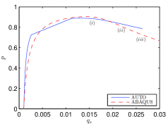
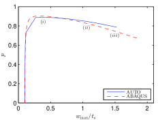
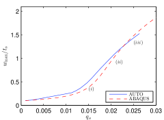
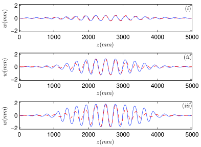
Figure 8: Comparison of the results from Auto (solid lines) with Abaqus (dashed lines) solutions. Normalized force $p$ versus amplitudes of (a) the global mode $q_{s}$ (b) the local mode $w_{\mathrm{max}}/t_{s}$. (c) local versus global mode amplitudes; (d) local buckling out-of-plane deflections $w$ of the stiffener for the points shown in (a–c) defined as (i)–(iii).

shows the comparisons between the analytical results from Auto-07p and the numerical results from Abaqus. This is shown for the case with an initial global imperfection ($W_{0}$) where $q_{s0}=0.001$ is combined with a local imperfection ($w_{0}$) where $A_{0}=0.12~{}\mathrm{mm}$, $\alpha=8.0$, $\beta=35$ and $\eta=L/2$, which matches the initial imperfection from Abaqus for the analytical model such that a meaningful comparison can be made. The graphs in (a–b) show the normalized axial load $p$ versus the buckling amplitudes of the global mode and the local deflection of the stiffener respectively. The graph in (c) shows the local versus the global buckling modal amplitudes; all three graphs show excellent correlation in all aspects of the mechanical response.

Figure 8(d) shows the local out-of-plane deflection profiles at the respective locations (i)–(iii) shown in Figure 8(a–c), the comparisons being for the same values of $q_{s}$. These, again, show excellent correlation between the results from Auto-07p and Abaqus, particularly near the peak load. A visual comparison between the 3-dimensional representation of the strut from the analytical and the FE models is also presented in Figure 9.

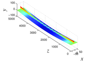
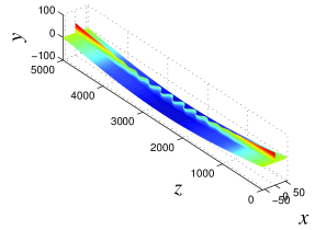
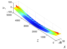
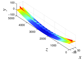
Figure 9: Numerical solutions from (left) Abaqus and (right) Auto visualized on 3-dimensional representations of the strut at the same load level: (a) $p=0.89$, (b) $p=0.84$, and (c) $p=0.81$ respectively). All dimensions are in millimetres, but the local buckling displacements in the stiffener are scaled by a factor of 5 to aid visualization.

The correlation with Abaqus, for a relatively high value of $c_{p}$, is seen to be excellent, but when $c_{p}$ is decreased the analytical model exhibits the characteristic snap-backs earlier (see Figures 4 and 7). However, the Abaqus solution for static post-buckling, which relies on assuming an initially imperfect geometry, does not (and indeed possibly cannot) obtain the progressive cellular buckling solution. This is not entirely surprising because the wavelength of the Abaqus solution seems to be fixed throughout the loading history. This demonstrates that for situations where buckling wavelengths are likely to change, the conventional method for analysing instability problems with static FE methods, where initial imperfections affine to a combination of eigenmodes are introduced and analysed using a nonlinear solver (e.g. the Riks method), may not be able to capture some experimentally observed physical phenomena. As an alternative, the authors attempted to model the problem as a dynamical system within Abaqus such that the snap-backs may be replicated more readily. However, computational issues in terms of slow and unreliable convergence stalled this study and it has been left for the future. Nevertheless, a recent study of a closely related structure [Wadee & Bai, 2013] clearly showed that the analytical approach matches the physical response significantly more accurately than static FE methods, in terms of the load versus displacement behaviour, and the observed change in the post-buckling wavelength. The observation of precisely the cellular buckling response has been reported for the flanges of thin-walled I-section struts experimentally [Becque, 2008], which is very similar to the current case where $h_{1}=h_{2}$ (see Figure 1). Hence, the authors are of the opinion that since cellular buckling is an observed physical phenomenon for those related structural components, the current results from the analytical model are also valid.

5 Concluding remarks

The current work identifies a form of cellular buckling in axially compressed stiffened plates. This arises from a potentially dangerous interaction of local and global modes of buckling, with a characteristic sequence of snap-back instabilities in the mechanical response. It is also found that the effect of the instabilities can be reduced somewhat by increasing the rotational stiffness of the joint between the main plate and the stiffeners. However, the mode interaction persists and the local buckling profile still changes wavelength, as has been found in recent related studies [Becque & Rasmussen, 2009, Wadee & Gardner, 2012, Wadee & Bai, 2013]. The increased rotational stiffness of the joint allows the model to be validated from a purely numerical formulation in FE software. However, earlier studies suggest that for smaller values of the aforementioned stiffness, the analytical model would be superior in modelling the actual physical response. This is in terms of the equilibrium response, the load-carrying capacity and the deformed shape, which is known from earlier research to exhibit the change in the local buckling wavelength. The latter point is crucial since the static FE solution seems to be unable to capture the changing wavelength of the post-buckling mode that has been observed in physical experiments. It is likely that in an actual scenario, the subcritical response in conjunction with the snap-backs are likely to lead to buckling cells being triggered dynamically. This has been observed during the tripping phenomenon [Ronalds, 1989] and the postulate is that the elastic interactive buckling found currently, if combined with plasticity, would promote this kind of sudden and violent collapse of a stiffened panel.

Currently, the authors are extending the analytical model by including the possibility of buckling the main plate in combination with the stiffener. In this case, the load-carrying capacity is likely to be reduced and it would be representative of a scenario where the cross-section has uniform thickness. Moreover, an imperfection sensitivity study is being conducted to quantify the parametric space for designers to avoid such dangerous structural behaviour.

References

- Abaqus, 2011 Abaqus. 2011. Version 6.10. Providence, USA: Dassault Systèmes.
- Becque, 2008 Becque, J. 2008. The interaction of local and overall buckling of cold-formed stainless steel columns. Ph.D. thesis, School of Civil Engineering, University of Sydney, Sydney, Australia.
- Becque & Rasmussen, 2009 Becque, J., & Rasmussen, K. J. R. 2009. Experimental investigation of the interaction of local and overall buckling of stainless steel I-columns. ASCE J. Struct. Eng., 135(11), 1340–1348. DOI: 10.1016/j.jcsr.2009.04.025.
- Budiansky, 1976 Budiansky, B. (ed). 1976. Buckling of structures. Berlin: Springer. IUTAM symposium.
- Burke & Knobloch, 2007 Burke, J., & Knobloch, E. 2007. Homoclinic snaking: Structure and stability. Chaos, 17(3), 037102. DOI: 10.1063/1.2746816.
- Butler et al., 2001 Butler, R., Lillico, M., Hunt, G. W., & McDonald, N. J. 2001. Experiments on interactive buckling in optimized stiffened panels. Struct. Multidisc. Optim., 23(1), 40–48. DOI: 10.1007/s00158-001-0164-0.
- Doedel & Oldeman, 2011 Doedel, E. J., & Oldeman, B. E. 2011. Auto-07p: Continuation and bifurcation software for ordinary differential equations. Montreal, Canada: Concordia University.
- Ghavami & Khedmati, 2006 Ghavami, K. G., & Khedmati, M. R. 2006. Numerical and experimental investigation on the compression behaviour of stiffened plates. J. Constr. Steel Res., 62(11), 1087–1100. DOI: 10.1016/j.jcsr.2006.06.026.
- Hunt & Wadee, 1998 Hunt, G. W., & Wadee, M. A. 1998. Localization and mode interaction in sandwich structures. Proc. R. Soc. A, 454(1972), 1197–1216. DOI: 10.1098/rspa.1998.0202).
- Hunt et al., 2000 Hunt, G. W., Peletier, M. A., Champneys, A. R., Woods, P. D., Wadee, M. A., Budd, C. J., & Lord, G. J. 2000. Cellular buckling in long structures. Nonlinear Dyn., 21(1), 3–29. DOI 10.1023/A:1008398006403.
- Hunt et al., 2003 Hunt, G. W., Lord, G. J., & Peletier, M. A. 2003. Cylindrical shell buckling: A characterization of localization and periodicity. Discrete Contin. Dyn. Syst.-Ser. B, 3(4), 505–518. DOI: 10.3934/dcdsb.2003.3.505.
- Koiter & Pignataro, 1976 Koiter, W. T., & Pignataro, M. 1976. A general theory for the interaction between local and overall buckling of stiffened panels. Tech. rept. WTHD 83. Delft University of Technology, Delft, The Netherlands.
- Murray, 1973 Murray, N. W. 1973. Buckling of stiffened panels loaded axially and in bending. Struct. Eng., 51(8), 285–300.
- Riks, 1979 Riks, E. 1979. An incremental approach to the solution of snapping and buckling problems. Int. J. Solids Struct., 15(7), 529–551. DOI: 10.1016/0020-7683(79)90081-7.
- Ronalds, 1989 Ronalds, B. F. 1989. Torsional buckling and tripping strength of slender flat-bar stiffeners in steel plating. Proc. Instn. Civ. Engrs., 87(Dec.), 583–604.
- Sheikh et al., 2002 Sheikh, I. A., Grondin, G.Y., & Elwi, A. E. 2002. Stiffened steel plates under uniaxial compression. J. Constr. Steel Res., 58(5-8), 1061–1080. DOI: 10.1016/S0143-974X(01)00083-9.
- Thompson & Hunt, 1973 Thompson, J. M. T., & Hunt, G. W. 1973. A general theory of elastic stability. London: Wiley.
- Wadee, 2000 Wadee, M. A. 2000. Effects of periodic and localized imperfections on struts on nonlinear foundations and compression sandwich panels. Int. J. Solids Struct., 37(8), 1191–1209. DOI: 10.1016/S0020-7683(98)00280-7.
- Wadee, 2002 Wadee, M. A. 2002. Localized buckling in sandwich struts with pre-existing delaminations and geometrical imperfections. J. Mech. Phys. Solids, 50(8), 1767–1787. DOI: 10.1016/S0022-5096(01)00132-6.
- Wadee & Bai, 2013 Wadee, M. A., & Bai, L. 2013. Cellular buckling in I-section struts. Thin-Walled Struct. In press. DOI: 10.1016/j.tws.2013.08.009.
- Wadee & Edmunds, 2005 Wadee, M. A., & Edmunds, R. 2005. Kink band propagation in layered structures. J. Mech. Phys. Solids, 53(9), 2017–2035. DOI: 10.1016/j.jmps.2005.04.005.
- Wadee & Gardner, 2012 Wadee, M. A., & Gardner, L. 2012. Cellular buckling from mode interaction in I-beams under uniform bending. Proc. R. Soc. A, 468(2137), 245–268. DOI: 10.1098/rspa.2011.0400.
- Wadee & Simões da Silva, 2005 Wadee, M. A., & Simões da Silva, L. A. P. 2005. Asymmetric secondary buckling in monosymmetric sandwich struts. Trans ASME J. Appl. Mech., 72(5), 683–690. DOI: 10.1115/1.1979513.
- Wadee et al., 2010 Wadee, M. A., Yiatros, S., & Theofanous, M. 2010. Comparative studies of localized buckling in sandwich struts with different core bending models. Int. J. Non-Linear Mech., 45(2), 111–120. DOI: 10.1016/j.ijnonlinmec.2009.10.001.
- Wadee et al., 1997 Wadee, M. K., Hunt, G. W., & Whiting, A. I. M. 1997. Asymptotic and Rayleigh–Ritz routes to localized buckling solutions in an elastic instability problem. Proc. R. Soc. A, 453(1965), 2085–2107. DOI: 10.1098/rspa.1997.0112.