Performance of PZF and MMSE Receivers in Cellular Networks with Multi-User Spatial Multiplexing

Abstract

This paper characterizes the performance of cellular networks employing multiple antenna open-loop spatial multiplexing techniques. We use a stochastic geometric framework to model distance depended inter cell interference. Using this framework, we analyze the coverage and rate using two linear receivers, namely, partial zero-forcing (PZF) and minimum-mean-square-estimation (MMSE) receivers. Analytical expressions are obtained for coverage and rate distribution that are suitable for fast numerical computation.

In the case of the PZF receiver, we show that it is not optimal to utilize all the receive antenna for canceling interference. With $\alpha$ as the path loss exponent, $N_{t}$ transmit antenna, $N_{r}$ receive antenna, we show that it is optimal to use $N_{t}\left\lceil\left(1-\frac{2}{\alpha}\right)\left(\frac{N_{r}}{N_{t}}-\frac{1}{2}\right)\right\rceil$ receive antennas for interference cancellation and the remaining antennas for signal enhancement (array gain). For both PZF and MMSE receivers, we observe that increasing the number of data streams provides an improvement in the mean data rate with diminishing returns. Also transmitting $N_{r}$ streams is not optimal in terms of the mean sum rate. We observe that increasing the SM rate with a PZF receiver always degrades the cell edge data rate while the performance with MMSE receiver is nearly independent of the SM rate.

I Introduction

Multiple-input multiple-output (MIMO) communication is an integral part of current cellular standards. The antennas can be used for increasing the number of data streams or improving the link reliability and the trade-off is well understood for a point-to-point link [1, 2, 3]. Spatial multiplexing (SM) is an important technique for boosting spectral efficiency of a point-to-point link with multiple antenna, wherein independent data streams are transmitted on different spatial dimensions. The capacity improvement with SM in an isolated link in the presence of additive Gaussian noise has been extensively studied [4, 5, 6].

However cellular systems are multi-user systems and co-channel interference is a major impediment to the network performance. Indeed, it has been argued with the help of simulations in [7, 8] that SM is not very effective in a multi-cell environment due to interference. In a multi-user setup, in addition to providing diversity and multiplexing, the antennas can also be used to serve different users and suppress interference, thereby adding new dimensions for system design.

Existing cellular networks employ both closed-loop and open-loop SM methods. Closed-loop SM requires channel state information (CSI) at the transmitter, and is suitable for users with slowly varying channels (low Doppler case). On the other hand open-loop SM is used for channels with high Doppler or in cases were there is inadequate feedback to support closed-loop SM. Open-loop SM is also used for increasing the performance of control channels where CSI feedback is not available. Open-loop SM can be implemented in two ways. In single user SM, a base station (BS) can allocate all the available data streams to a single user thereby increase the user’s rate. Alternatively, the BS can serve multiple users at the same time by allocating one stream per user. The latter approach is termed as open-loop multi-user SM.

We consider the case where each BS has $N_{t}$ antenna and multiplexes $N_{t}$ streams with one stream per user. The receiver has $N_{r}$ receiver antennas. In this case, with a linear receiver, $N_{t}$ degrees-of-freedom (DOF) (among available $N_{r}$ DOF) can be used for suppressing self-interference caused by SM while the remaining $N_{r}-N_{t}$ DOF can be used for suppression of other cell interference or to obtain receiver array gain. For a typical cell edge user, a reduction of the SM rate at the transmitter might result in enough residual DOF (after suppression of self-interference) to cancel the other cell interference and generally results in an increased throughput. When the number of data streams transmitted from a BS is less than the number of antennas available, techniques like cyclic-delay-diversity or open-loop dumb-beamforming [9] can be used the remaining antennas.

In this paper, we consider distance dependent inter-cell interference and investigate how multiple antenna can be used in the down link of an open-loop cellular system. A general design goal is to maximize both mean and cell edge data rates. We analyze the various trade-offs between SM rate and the achievable mean/cell-edge data rates using linear receivers.

II Related Work

Recent studies [7, 8] show that spatial multiplexing MIMO systems, whose main benefit is the supposed potential upswing in spectral efficiency, lose much of their effectiveness in a multi-cell environment with high interference. Several approaches to handling interference in multi-cell MIMO systems are discussed in [8]. Blum in [10] investigated the capacity of an open-loop multi user MIMO system with interference and have shown that the optimum power allocation across antenna depends on the interference power. When the interference is high, it is optimal to allocate the entire power to one transmit antenna (single-stream) rather than spreading the power equally across antenna.

There has been considerable work in ad hoc networks contrasting single stream transmission with multi-stream transmission using tools from stochastic geometry. It has been shown in [11, 12] that the network-wide throughput can be increased linearly with the number of receive antennas, even if only a single transmit antenna is used by each node, and each node sends/receives only a single data stream. Interestingly, no channel state information (CSI) is required at the transmitter to achieve this gain.

Using $(1-2/\alpha)$, where $\alpha$ is the path loss exponent, fraction of the receive degrees of freedom for interference cancellation and the remaining degrees of freedom for array gain, allows for a linear scaling of the achievable rate with the number of receiving antennas [12]. It is interesting to see that canceling merely one interferer by each node may increase the transmission capacity even when the CSI is imperfect [13]. Importance of interference cancellation in ad-hoc networks is also discussed in [14, 15] and [16]. However, most of these results are obtained by deriving bounds on the signal-to-interference ratio ($\mathtt{SIR}$) distribution.

In [17, 18] the exact distribution of $\mathtt{SIR}$ with SM and minimum-mean-square-estimation (MMSE) receiver has been obtained in an ad hoc network when the interferers are distributed as a spatial Poisson point process. The $\mathtt{SIR}$ follows a quadratic form, and results from [19, 20] are used to obtain the distribution. Again, it was shown that single-stream transmission is preferable over multi-stream transmission. In [21], distribution of $\mathtt{SIR}$ for multiple antenna system with various receivers and transmission schemes are obtained for a Poisson interference field. In [16] scaling laws for the transmission capacity with zero-forcing beamforming were obtained, and it was shown that for a large number of antennas, the maximum density of concurrently transmitting nodes scales linearly with the number of antennas at the transmitter, for a given outage constraint. In [22], the distribution of $\mathtt{SIR}$ in a zero-forcing receiver with co-channel interference is obtained.

In ad hoc networks, an interferer can be arbitrarily close (much closer than the intended transmitter) to the receiver in consideration. This results in interference that is heavy-tailed. On the other hand, in a cellular network the user usually connects to the closest BS and hence the distance to the nearest interferer is greater than the distance to the serving BS. This leads to a more tamed interference distribution compared to an ad hoc networks.

II-A Main Contributions

In this paper we focus on linear receivers, namely the the partial zero-forcing receiver and the MMSE receiver. The MMSE receiver optimally balances signal boosting and interference cancellation and maximizes the SINR. The sub-optimal partial zero-forcing receiver uses a specified number of degrees of freedom for signal boosting and the remainder for interference cancellation.

• We provide the distribution of $\mathtt{SINR}$ with a partial zero-forcing receiver. This analysis also includes the inter-cell interference which is usually neglected. The resultant expression can be computed by evaluating a single integral.

• With one stream per-user, we obtain the optimal configuration of receive antennas. In particular we show that it is optimal to use $N_{t}\left\lceil\left(1-\frac{2}{\alpha}\right)\left(\frac{N_{r}}{N_{t}}-\frac{1}{2}\right)\right\rceil$ receive antennas for interference cancellation and the remaining antennas for signal enhancement (array-gain).

• We compute the cumulative distribution function of the $\mathtt{SINR}$ with a linear MMSE receiver. In the interference-limited case, the distribution can be computed without any integration.

• The sum rate expressions are provided for both PZF and MMSE receivers. Numerical evaluation of these results show that average sum rate increases with the number of data streams with diminishing returns. The mean sum rate reaches a maximum value for a certain optimum number of data stream that is generally less than the number of receive antenna $N_{r}$. On the other hand, increasing the number of data streams always degrades the cell edge data rate for PZF receiver and MMSE receivers. However, the impact is less severe with a MMSE receiver.

II-B Organization of the paper

In Section III, the system model, particularly the BS location model, is described in detail. In Section IV, the $\mathtt{SINR}$ distribution with a partial-zero-forcing receiver is derived. In Section V, the $\mathtt{SINR}$ distribution is obtained for a linear MMSE receiver and in Section VI, the average ergodic rate is analyzed with both PZF and MMSE receivers. The paper is concluded in Section VII.

III System Model

We now provide a mathematical model of the cellular system that will be used in the subsequent analysis. We begin with the spatial distribution of the base stations.

Network Model: The locations of the base stations (BSs) are modeled by a spatial Poisson point process (PPP) [23] $\Phi\subset\mathbb{R}^{2}$ of density $\lambda$. The PPP model for BS spatial location provides a good approximation for irregular BS deployments. The merits and demerits of this model for BS locations have been extensively discussed in [24].

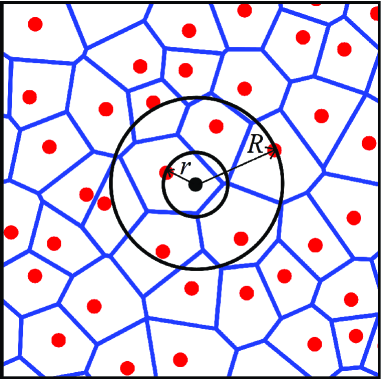
We assume the nearest BS connectivity model, i.e., a user connects to the nearest BS. This nearest BS connectivity model results in a Voronoi tessellation of the plane with respect to the BS locations. See Figure 1. Hence the service area of a BS is the Voronoi cell associated with it.

We assume that each BS is equipped with $N_{t}$ antenna (active transmitting antennas) and a user (UE) is equipped with $N_{r}$ antenna. In this paper we focus on downlink and hence the $N_{t}$ antenna at the BSs are used for transmission and the $N_{r}$ antenna at the UE are used for reception. We assume that all the BSs transmit with equal power which for convenience we set to unity. Hence each transmit antenna uses a power of $1/N_{t}$.

Channel and path loss model: We assume independent Rayleigh fading with unit mean between any pair of antenna. We focus on the downlink performance and hence without loss of generality, we consider and analyse the performance of a typical mobile user located at the origin. The $N_{r}\times 1$ fading vector between the $q$-th antenna of the BS $x\in\Phi$ and the typical mobile at the origin is denoted by $\mathbf{h}_{x,q}$. We assume $\mathbf{h}_{x,q}\sim\mathcal{CN}(\mathbf{0}_{N_{r}\times 1},\mathbf{I}_{N_{r}})$, i.e., a circularly-symmetric complex Gaussian random vector. The standard path loss model $\ell(x)=\|x\|^{-\alpha}$, with path loss exponent $\alpha>2$ is assumed. Specifically, the link between $q$-th transmit antenna of the BS at $x$ and the $N_{r}$ receiver antennas of the user at origin is $\sqrt{\|x\|^{-\alpha}}\mathbf{h}_{x,q}$.

Received signal and interference: We consider the case where each BS uses its $N_{t}$ antennas to serve $N_{t}$ independent data streams to $N_{t}$ users in its cell. Let $\hat{o}\in\Phi$ denote the BS that is closest to the mobile user at the origin. We assume that the UE at the origin is interested in decoding the $k$-th stream transmitted by its associated BS $\hat{o}$. Focusing on the $k$-th stream transmitted by $\hat{o}$, the received $N_{r}\times 1$ signal vector at the typical mobile user is

$$\mathbf{y}= \frac{a_{\hat{o},k}}{\sqrt{r^{\alpha}}}\mathbf{h}_{\hat{o},k}+\frac{1}{\sqrt{r^{\alpha}}}\sum_{q=1,q\neq k}^{N_{t}}\mathbf{h}_{\hat{o},q}a_{\hat{o},q}+\mathbf{I}(\Phi)+\mathbf{w},$$ (1)

where $\mathbf{I}(\Phi)=\sum_{x\in\Phi\setminus\hat{o}}\frac{1}{\sqrt{\|x\|^{\alpha}}}\sum_{q=1}^{N_{t}}\mathbf{h}_{x,q}a_{x,q}$, denotes the intercell interference from other BSs. The symbol transmitted from the the $q$-th antenna of the base station $x\in\Phi$ is denoted by $a_{x,q}$ and $\mathbb{E}[|a_{x,q}|^{2}]=1/N_{t}$. The additive white Gaussian noise is given by $\textbf{w}\sim\mathcal{CN}(\mathbf{0}_{N_{r}\times 1},\sigma^{2}\mathbf{I}_{N_{r}})$. The distance between the typical mobile user at the origin and its associated (closest) BS is denoted by $r=\|\hat{o}\|$. Observe that $r$ is a random variable since the BS locations are random. We now present few auxiliary results on the distribution of some spatial random variables that will be used later in the paper.

Figure 1: Illustration of the BS locations modelled by a PPP and their corresponding cells. As an example, the distance to the fifth nearest BS from the typical user at the origin is denoted by $R$ and the distance to the serving BS is denoted by $r$.

Distance to the serving BS and $(m-1)$-th interfering BS: We now obtain the joint distribution of the distance of the origin to the nearest BS and the distance to the $m-1$ interfering BS. Recall that $r$ denotes the distance to the serving (nearest) BS. The PDF of the distance to the nearest neighbor is [23]

$$f_{r}(r)=e^{-\lambda\pi r^{2}}2\pi\lambda r.$$ (2)

We now compute the distance to the $(m-1)$-th closest interfering BS conditioned on the distance to the nearest BS $r$. Let $R$ denote the distance to the $(m-1)$-th BS. See Figure 1. Hence the event $R\leq R_{0}$ equals the event that there are at least $m-1$ base stations in the region between two concentric circles of radius $r$ and $R$ centred at origin. Hence

$$F_{R|r}(R_{0}\ |\ r_{0})= \>\mathbb{P}\left[R\leq R_{0}|r=r_{0}\right]=\sum_{k=m-1}^{\infty}e^{-\pi\lambda(R_{0}^{2}-r_{0}^{2})}\displaystyle\frac{[\lambda\pi(R_{0}^{2}-r_{0}^{2})]^{k}}{k!},\ R_{0}>r_{0}.$$ (3)

Hence the conditional PDF is

$$f_{R|r}(R|r)= \frac{2\pi\lambda R}{(m-2)!}e^{-\pi\lambda(R^{2}-r^{2})}\left(\pi\lambda(R^{2}-r^{2})\right)^{m-2},\ R>r.$$ (4)

Let $\beta=R/r$ denote the ratio of the distance of the $m-1$ th closest interfering BS of the typical user to the distance of its closest BS. Using (4) and (2), it can be easily shown that the PDF of the random variable $\beta$ is

$$g_{\beta}(\beta)=2(m-1)\beta^{1-2m}(\beta^{2}-1)^{m-2},\ \beta>1.$$ (5)

Observe that the ration $\beta$ does not depend on the density of the PPP. The average value of $\beta$ is given by $\mathbb{E}[\beta]=\frac{\sqrt{\pi}\Gamma(m)}{\Gamma(m-1/2)}\approx\sqrt{(m-1)\pi}$, and $\mathbb{E}[\beta^{\nu}]=\infty,\ \nu\geq 2$ irrespective of $m\geq 2$. We begin with the analysis of a partial zero forcing receiver.

IV Partial zero forcing (PZF) receiver

In this section, we will analyze the distribution of the post-processing $\mathtt{SINR}$ with a PZF receiver in a cellular setting. We assume that the user has perfect knowledge of the interfering node channels that it wishes to cancel.

IV-A Coverage probability

Each user has $N_{r}$ antenna, which can be represented as $N_{r}=mN_{t}+\delta$, $m\geq 1$ receive antenna. The receive filter $\mathbf{v}$ for the typical user at the origin is chosen orthogonal to the channel vectors of the interferers and the streams that need to be canceled. Without loss of generality, we assume that the typical UE at the origin is interested in the $k$-th stream (1). The receive filter $\mathbf{v}$ is chosen as a unit norm vector orthogonal to the following vectors:

$$\mathbf{h}_{\hat{o},q} :q=1,2,..,k-1,k+1,..,N_{t},$$

$$\mathbf{h}_{x,q} :x\in\{x_{1},x_{2},...,x_{m-1}\},\ q=1,2,..,N_{t},$$

where $\{x_{1},x_{2},...,x_{m-1}\}$ are the $(m-1)$ BSs closest to the typical UE in consideration excluding $\hat{o}$. The dimension of the span of the above mentioned vectors is $N_{t}-1+(m-1)N_{t}=mN_{t}-1$ with high probability. Amongst the filters orthogonal to those vectors, we are interested in the one that maximizes the signal power $|\mathbf{v}^{\dagger}\mathbf{h}_{\hat{o},k}|^{2}$ . This corresponds to choosing $\mathbf{v}$ in the direction of the projection of vector $\mathbf{h}_{\hat{o},k}$ on the nullspace of the interfering channel vectors. The dimension of the corresponding nullspace is $N_{r}-mN_{t}+1$. If the columns of an $(N_{r}-mN_{t}+1)\times N_{r}$ matrix $\mathbf{Q}$ form an orthonormal basis for this nullspace, then the receive filter $\mathbf{v}$ is chosen as:

$$\mathbf{v}=\mathbf{Q}\frac{\mathbf{Q}^{\dagger}\mathbf{h}_{\hat{o},k}}{\|\mathbf{Q}^{\dagger}\mathbf{h}_{\hat{o},k}\|}.$$

So if $N_{r}=mN_{t}+\delta$, the remaining $\delta+1$ degrees of freedom can be used to boost the signal power. Hence at the receiver,

$$\mathbf{v}^{\dagger}\mathbf{y}_{k}= \frac{a_{\hat{o},k}}{\sqrt{r^{\alpha}}}\mathbf{v}^{\dagger}\mathbf{h}_{\hat{o},k}+\sum_{q=1,q\neq k}^{N_{t}}\frac{a_{\hat{o},q}}{\sqrt{r^{\alpha}}}\mathbf{v}^{\dagger}\mathbf{h}_{\hat{o},q}+\mathbf{v}^{\dagger}\mathbf{I}(\Phi)+\mathbf{v}^{\dagger}\mathbf{w}.$$

Since $\mathbf{v}^{\dagger}$ is designed to null the closest $m-1$ interferers, $\mathbf{v}^{\dagger}\mathbf{I}(\Phi)=\mathbf{v}^{\dagger}\mathbf{I}(\hat{\Phi})$ where $\hat{\Phi}=\Phi\setminus\{x_{1},...,x_{m-1}\}$. So we have $\tilde{y}_{k}=\frac{a_{\hat{o},k}}{\sqrt{r^{\alpha}}}\mathbf{v}^{\dagger}\mathbf{h}_{\hat{o},k}+\mathbf{v}^{\dagger}\mathbf{I}(\hat{\Phi})+\mathbf{v}^{\dagger}\mathbf{w}$. Let $S\overset{\triangle}{=}|\mathbf{v}^{\dagger}\mathbf{h}_{\hat{o},k}|^{2}$ and $H_{x,q}\overset{\triangle}{=}|\mathbf{v}^{\dagger}\mathbf{h}_{x,q}|^{2}$. The post processing zero-forcing signal-to-interference-noise ratio ($\mathtt{SINR}$) [11] of the $k$-th stream is

$$\mathtt{SINR}= \frac{Sr^{-\alpha}}{N_{t}\sigma^{2}+\underbrace{\sum_{x\in\hat{\Phi}}\|x\|^{-\alpha}\sum_{q=1}^{N_{t}}H_{x,q}}_{\hat{\mathbf{I}}(\hat{\Phi})}}.$$ (6)

Also $S\sim\chi^{2}_{2(N_{r}-mN_{t}+1)}$, i.e., a chi-squared random variable with $2(N_{r}-mN_{t}+1)$ degrees of freedom and $H_{x,q}$ are i.i.d. exponential random variables. When $N_{r}=mN_{t}$ the receiver can only cancel interference from $(m-1)$ nearest BSs and in this case, $S$ is an exponential random variable.

A mobile user is said to be in coverage if the received $\mathtt{SINR}$ (after pre-processing) is greater than the threshold $z$, needed to establish the connection. The probability of coverage is defined as

$$\mathtt{P}_{\mathtt{PZF}}(z)\overset{\triangle}{=}\mathbb{P}[\mathtt{SINR}>z].$$ (7)

Observe that the coverage is essentially the complementary cumulative distribution function (CCDF) of the $\mathtt{SINR}$. Since $\mathtt{P}_{\mathtt{PZF}}(z)$, quantifies the entire distribution, it can be used to compute other metrics of interest like average ergodic rate. We first provide the main result which deals with the coverage probability with noise. We begin with the evaluation of the Laplace transform of interference conditioned on the distances $R$ and $r$.

Lemma 1.

The Laplace transform of the residual interference in PZF conditional on $R$ and $r$ is given by

$$\mathcal{L}_{\mathbf{I}}(s)=\exp\left(-\lambda\pi R^{2}\left(\,{}_{2}F_{1}\left(N_{t},-\frac{2}{\alpha},\frac{\alpha-2}{\alpha},-R^{-\alpha}s\right)-1\right)\right),$$

where ${}_{2}F_{1}(a,b,c,z)$ is the standard hypergeometric function.

Proof.

The PZF receiver is designed such that it can cancel interference from nearest $(m-1)$ BSs. Conditioned on the distance to $(m-1)$-th BS $R$,

$$\mathcal{L}_{\mathbf{I}}(s)= \mathbb{E}\left[e^{-s\hat{\mathbf{I}}(\hat{\Phi})}\right]=\mathbb{E}\exp\left(-s\sum_{x\in\hat{\Phi}}\|x\|^{-\alpha}\sum_{q=1}^{N_{t}}H_{x,q}\right).$$

Since $H_{x,q}$ are i.i.d exponential, their sum $\sum_{q=1}^{N_{t}}H_{x,q}$ is Gamma distributed. Using the Laplace transform of the Gamma distribution,

$$\mathcal{L}_{\mathbf{I}}(s)= \mathbb{E}\prod_{x\in\hat{\Phi}}\mathbb{E}\exp\left(-s\|x\|^{-\alpha}\sum_{q=1}^{N_{t}}H_{x,q}\right)=\mathbb{E}\prod_{x\in\hat{\Phi}}\frac{1}{(1+s\|x\|^{-\alpha})^{N_{t}}},$$

$$\stackrel{{\scriptstyle(a)}}{{=}} \exp\left(-\lambda 2\pi\int_{R}^{\infty}\left(1-\frac{1}{(1+sx^{-\alpha})^{N_{t}}}\right)x\mathrm{d}x\right),$$

$$= \exp\left(-\lambda\pi R^{2}\left(\,{}_{2}F_{1}\left(N_{t},-\frac{2}{\alpha},\frac{\alpha-2}{\alpha},-R^{-\alpha}s\right)-1\right)\right).$$ (8)

where $(a)$ follows from the probability generating functional (PGFL) of the PPP [23]. ∎

The Laplace transform in Lemma 2 is used next to compute the coverage probability.

Theorem 1.

The probability of coverage with PZF receiver having $N_{r}=mN_{t}+\delta$ antennas is given by

$$\mathtt{P}_{\mathtt{PZF}}(z)=\int_{0}^{\infty}\int_{r}^{\infty}\sum_{k=0}^{\delta}\frac{(-s)^{k}}{k!}\frac{\mathrm{d}^{k}}{\mathrm{d}s^{k}}\mathcal{L}_{\mathbf{I}}(s)e^{-sN_{t}\sigma^{2}}\Big{|}_{s=zr^{\alpha}}f_{R|r}(R|r)f_{r}(r)\mathrm{d}R\mathrm{d}r,$$

where $\mathcal{L}_{\mathbf{I}}(s)$ is given in Lemma 2 and $f_{R|r}(R|r)$ in (4).

Proof.

Conditioned on the random variables $R$ and $r$, we have

$$\mathtt{P}_{c}(z,\alpha\ |\ r)= \mathbb{E}_{\mathbf{I}}[\mathbb{P}(S>z\,r^{\alpha}(\mathbf{I}+N_{t}\sigma^{2}))],$$

$$\overset{(a)}{=} \sum_{k=0}^{\delta}\frac{({z\,r^{\alpha}})^{k}}{k!}\mathbb{E}_{\mathbf{I}}[(\mathbf{I}+N_{t}\sigma^{2})^{k}e^{-zr^{\alpha}(\mathbf{I}+N_{t}\sigma^{2})}],$$

$$\overset{(b)}{=} \sum_{k=0}^{\delta}\left(\frac{(-s)^{k}}{k!}\frac{\mathrm{d}^{k}}{\mathrm{d}s^{k}}\mathcal{L}_{(\mathbf{I}+N_{t}\sigma^{2})}(s)\right)_{s=zr^{\alpha}}.$$ (9)

$(a)$ follows from the CCDF of $\chi_{2(N_{r}-mN_{t}+1)}^{2}$ and $(b)$ by the differentiation property of the Laplace transform. $\mathcal{L}_{(\mathbf{I}+N_{t}\sigma^{2})}(s)$ is the Laplace transform of interference and noise and equals $\mathcal{L}_{\mathbf{I}}(s)\exp(-sN_{t}\sigma^{2})$ where $\mathcal{L}_{\mathbf{I}}(s)$ is given in Lemma 2. The result follows by averaging over $R$ and $r$. ∎

IV-B Interference limited networks, $\sigma^{2}=0$

We now specialize the coverage expression in Theorem 1 when $\sigma^{2}=0$, i.e., an interference-limited network. In Theorem 1, the coverage probability expression requires evaluating the $k$-th derivative of a composite function. The derivatives of a composite function can be written in a succinct form by using a set partition version of Faà di Bruno’s formula. We now introduce some notation that will be used in the next theorem.

A partition of a set $S$ is a collection of disjoint subsets of $S$ whose union is $S$. The collection of all the set partitions of the integer set $[1,2,3,\ldots k]$ is denoted by $\mathcal{S}_{k}$ and its cardinality is called the $k$-th Bell number. For a partition $\upsilon\in\mathcal{S}_{k}$, let $|\upsilon|$ denote the number of blocks in the partition and $|\upsilon|_{j}$ denote the number of blocks with exactly $j$ elements. For example, when $k=3$, there are $5$ partitions,

$$\mathcal{S}_{3}=\Big{\{}\{1,2,3\},\big{\{}\{1\},\{2,3\}\big{\}},\big{\{}\{1,2\},\{3\}\big{\}},\big{\{}\{1,3\},\{2\}\big{\}},\big{\{}\{1\},\{2\},\{3\}\big{\}}\Big{\}}.$$

For the partition $\upsilon=\big{\{}\{1\},\{2\},\{3\}\big{\}}$, $|\upsilon|=3$, $|\upsilon|_{1}=3$ and $|\upsilon|_{2}=0$. Also, define

$$\Lambda_{\varsigma,N_{t}}(z)\triangleq\,_{2}F_{1}\left(N_{t}+\varsigma,\varsigma-\frac{2}{\alpha},\varsigma-\frac{2}{\alpha}+1,-z\right),$$

where $\,{}_{2}F_{1}(a,b,c,x)$ is the standard hypergeometric function.

Theorem 2.

When the network is interference limited, i.e., $\sigma^{2}=0$, the probability of coverage with a PZF receiver having $N_{r}=mN_{t}+\delta$ antennas is

$$\mathtt{P}_{\mathtt{PZF}}(z)= \sum_{k=0}^{\delta}\frac{z^{k}}{k!}\sum_{\upsilon\in\mathcal{S}_{k}}(-1)^{|\upsilon|}(m)_{|\upsilon|}\mathbb{E}_{\beta}\left[{\frac{\beta^{-\alpha k}}{\Lambda_{0,N_{t}}(\beta^{-\alpha}z)^{m}}\prod_{j=1}^{k}\left(\frac{(N_{t})_{j}(-\frac{2}{\alpha})_{j}}{(\frac{\alpha-2}{\alpha})_{j}}\frac{\Lambda_{j,N_{t}}(\beta^{-\alpha}z)}{\Lambda_{0,N_{t}}(\beta^{-\alpha}z)}\right)^{|\upsilon|_{j}}}\right],$$ (10)

where, $(x)_{n}=\frac{\Gamma(x+n)}{\Gamma(n)}$ is the Pochhammer function., The expectation is with respect to the variable $\beta=R/r$ whose PDF is given by $g(\beta)$ provided in (5)

Proof.

See Appendix A. ∎

In Table I, the coverage probability expressions are provided for the case of $m=2$. We now make a few observations:

• When $m=1$, i.e., only the self-interference from the other data streams is canceled, $\beta=1$ almost surely and hence the expectation with respect to $\beta$ in Theorem 2 can be dropped.

• When $\delta=0$, i.e., all the antenna are used to cancel interference, then

  $$\mathtt{P}_{\mathtt{PZF}}(z)=\mathbb{E}_{\beta}[\Lambda_{0,N_{t}}(\beta^{-\alpha}z)^{-m}].$$

  From the expression, it seems that the coverage probability increases exponentially with the number of canceled interferers. However, this is not the case as $\beta$ in the above expression is a function of $m$. This can be seen in Figure 2 where we observe diminishing benefits with increasing $m$

  Figure 2: Coverage probability versus $m$ for various $N_{t}$ with $\alpha=4$ at $z=0$ dB.

• In Theorem 2, the coverage probability is obtained by averaging over $\beta=R/r$. Hence $\mathtt{P}_{\mathtt{PZF}}(z)$ corresponds to the coverage probability of typical user. Instead of averaging over $\beta$, evaluating (22) at a particular value of $\beta$ would indicate the coverage of a user at a specified distance. For example, $\beta=1$ would correspond to an edge user with $m=2$.

$N_{t}\times N_{r}$	Coverage probability $\mathtt{P}_{\mathtt{PZF}}(z)$
$1\times 2$	$\int_{\beta=1}^{\infty}\frac{2}{\beta^{3}\,_{2}F_{1}\left(1,-\frac{2}{\alpha};1-\frac{2}{\alpha};-z\beta^{-\alpha}\right){}^{2}}\mathrm{d}\beta$.
$1\times 3$	$\int_{\beta=1}^{\infty}\frac{2}{\beta^{3}\,_{2}F_{1}\left(1,-\frac{2}{\alpha};1-\frac{2}{\alpha};-z\beta^{-\alpha}\right){}^{2}}-\frac{4z\beta^{-\alpha-3}\Gamma\left(1-\frac{2}{\alpha}\right)^{2}\,_{2}F_{1}\left(2,1-\frac{2}{\alpha};2-\frac{2}{\alpha};-z\beta^{-\alpha}\right)}{\Gamma\left(2-\frac{2}{\alpha}\right)\Gamma\left(-\frac{2}{\alpha}\right)\,_{2}F_{1}\left(1,-\frac{2}{\alpha};1-\frac{2}{\alpha};-z\beta^{-\alpha}\right){}^{3}}\mathrm{d}\beta$.
$2\times 4$	$\int_{\beta=1}^{\infty}\frac{2}{\beta^{3}\,_{2}F_{1}\left(2,-\frac{2}{\alpha};1-\frac{2}{\alpha};-z\beta^{-\alpha}\right){}^{2}}\mathrm{d}\beta$.
$2\times 5$	$\int_{\beta=1}^{\infty}\frac{2}{\beta^{3}\,_{2}F_{1}\left(2,-\frac{2}{\alpha};1-\frac{2}{\alpha};-z\beta^{-\alpha}\right){}^{2}}-\frac{8z\beta^{-\alpha-3}\Gamma\left(1-\frac{2}{\alpha}\right)^{2}\,_{2}F_{1}\left(3,1-\frac{2}{\alpha};2-\frac{2}{\alpha};-z\beta^{-\alpha}\right)}{\Gamma\left(2-\frac{2}{\alpha}\right)\Gamma\left(-\frac{2}{\alpha}\right)\,_{2}F_{1}\left(2,-\frac{2}{\alpha};1-\frac{2}{\alpha};-z\beta^{-\alpha}\right){}^{3}}\mathrm{d}\beta$.

TABLE I: Coverage probability expressions for $\sigma^{2}=0$, $m=2$ with different $N_{t}$.

IV-C Interference cancellation or signal enhancement?

The antennas at the receiver can be used for either interference cancellation or enhancing the desired signal. In our formulation, $mN_{t}-1$ antenna are used for interference cancellation while $\delta+1$ antenna are used for signal enhancement. For a given $N_{r}$, what is the optimal $(m,\delta)$ split to maximize the coverage probability? Since coverage probability is a complicated expression of $(m,\delta)$, we will use the average interference-to-signal ratio as the metric. We have

$$\mathbb{E}[\mathtt{SINR}^{-1}]=\mathbb{E}[N_{t}\sigma^{2}r^{\alpha}S^{-1}+S^{-1}\mathbf{I}r^{\alpha}],$$

which equals $N_{t}\sigma^{2}\mathbb{E}[r^{\alpha}]\mathbb{E}[S^{-1}]+\mathbb{E}[S^{-1}]\mathbb{E}[\mathbf{I}r^{\alpha}]]$. If $\delta\neq 0$, then $\mathbb{E}[S^{-1}]=\frac{1}{2\delta}$. Since $r$ is Rayleigh distributed, $\mathbb{E}[r^{\alpha}]=(\pi\lambda)^{-\alpha/2}\Gamma(1+\alpha/2)$. Also, $\mathbb{E}[\mathbf{I}r^{\alpha}]=N_{t}\sum_{k=m}^{\infty}\mathbb{E}[\beta^{-\alpha}_{(k)}]$, where $\beta_{(k)}$ represent the ratio of the distance to the $k$-th nearest interfering station to the serving BS distance. Using (5), we obtain

$$\mathbb{E}[\mathbf{I}r^{\alpha}]=N_{t}\sum_{k=m}^{\infty}{(k-1)\Gamma(k-1)\Gamma(1+\alpha/2)}{\Gamma(k+\alpha/2)^{-1}}.$$

Hence

$$\mathbb{E}[\mathtt{SINR}^{-1}]=\frac{N_{t}\Gamma(1+\alpha/2)}{2\delta}\left(\sigma^{2}(\pi\lambda)^{-\alpha/2}\Gamma(1+\alpha/2)+\sum_{k=m}^{\infty}\frac{\Gamma(k)\Gamma(1+\alpha/2)}{\Gamma(k+\alpha/2)}\right).$$ (11)

It follows from Kershaw’s inequality that $\Gamma(k+\alpha/2)/\Gamma(k)\approx(k+\alpha/4-1/2)^{\alpha/2}$ (indeed an upper bound). Substituting for $\Gamma(k+\alpha/2)/\Gamma(k)$ and replacing the summation by integration, we have the following approximation:

$$\mathbb{E}[\mathtt{SINR}^{-1}]\approx\frac{N_{t}\Gamma(1+\frac{\alpha}{2})}{2\delta}\left(\sigma^{2}(\pi\lambda)^{-\frac{\alpha}{2}}\Gamma(1+\frac{\alpha}{2})+\frac{2\Gamma(1+\frac{\alpha}{2})(m+\frac{\alpha}{4}-1/2)^{1-\frac{\alpha}{2}}}{\alpha-2}\right).$$ (12)

Using this result we can obtain the optimal $m$ and is stated in the following proposition.

Figure 3: Average $\mathbb{E}[\mathtt{SINR}^{-1}]$ from (11) as a function of $m$ for $N_{r}=10$ with different $N_{t}$ and $\alpha$ for $\sigma^{2}=0$. The optimal (lowest) value in each case is marked. We observe that the optimal value is always $N_{t}\left\lceil\left(1-\frac{2}{\alpha}\right)\left(\frac{N_{r}}{N_{t}}-\frac{1}{2}\right)\right\rceil$ as specified in Proposition 1.

Proposition 1.

The optimal $m^{*}(\sigma^{2})$ is the smallest integer that is greater than the positive root of the equation

$$2(m+\alpha/4-1/2)^{1-\alpha/2}N_{t}+\sigma^{2}(\pi\lambda)^{-\alpha/2}N_{t}(\alpha-2)-(N_{r}-mN_{t})(m+\alpha/4-1/2)^{-\alpha/2}(\alpha-2)=0,$$

if such a root exists. In particular when $\sigma^{2}=0$, i.e., when the system is interference limited, we have

$$m^{*}(0)=N_{t}\left\lceil\left(1-\frac{2}{\alpha}\right)\left(\frac{N_{r}}{N_{t}}-\frac{1}{2}\right)\right\rceil.$$ (13)

Proof.

To find the optimal $m$, we set $\delta=N_{r}-mN_{t}$ in (12), differentiate and equate to zero. ∎

This is in tune with the results in [11], where they show that it is optimal to use $(1-2/\alpha)$ fraction of the antennas for interference cancellation. In Figure 3, the average $\mathbb{E}[\mathtt{SINR}^{-1}]$ computed using (11) is plotted as a function of $m$ for various configurations. We observe that the optimal $m^{*}(0)$ coincides with the optimal $m$ as can be seen in the Figure 3. This result indicates that it is optimal to utilize $m^{*}(0)$ fraction of receive antenna to cancel interfering nodes and utilize the remaining antenna to strengthen the desired signal. So as the path loss exponent $\alpha$ increases, more antenna should be used for interference cancellation rather than boosting the desired signal.

IV-D Numerical results for coverage and discussion

Figure 4: Coverage probability versus $z$ for $N_{r}=4$ and different $N_{t}$ with optimal choice of $m$. The path loss exponent $\alpha=4$ and $\sigma^{2}=0$. Coverage probability versus $z$ for different choices of $m$ and $\delta$. The path loss exponent $\alpha=4$ and $\sigma^{2}=0$. The Monte Carlo results are also plotted and marked with $\oplus$. For $N_{t}\times N_{r}=1\times 4$ and $\alpha=4$, from (13), $m^{*}(0)=2$.

In Figure 4, the coverage probability is plotted for $1\times 4$ configuration for $\alpha=4$ and different choices of $m$ and $\delta$ using Theorem 2. In the same Figure, the coverage results for different configurations obtained by Monte Carlo simulation are marked by $\oplus$. We first observe that the coverage results obtained with Monte Carlo simulations match with the analytical results.

We observe that utilizing all the antennas for interference cancellation is not optimal. In fact, from Figure 4, we observe that utilizing all the antenna for interference cancellation leads to the lowest coverage probability, particularly for medium $\mathtt{SIR}$ thresholds.

If a very high $\mathtt{SIR}$ is required, we observe from Figure 4 that it is better to use all the antenna for cancellation. This can be observed by looking at the crossover points of the different curves. So an interior user should use his antenna to cancel interferers and obtain a higher $\mathtt{SIR}$. For most users, canceling the strongest interference improves the coverage significantly over the ZF receiver which utilizes all of its receiver DoF to cancel interference. So in a practical system, obtaining the channel of the nearest interferer is sufficient to have good coverage. It can also be seen that canceling nearest three BSs is giving almost same coverage compared to canceling nearest two, the reason is that the interference from the third may not be strong enough. So the better strategy can be canceling nearest BSs and using the remaining DoF for array gain. We also observe that canceling one interferer, i.e., $m=2$ has the highest coverage probability and corresponds to $m^{*}(0)$ for $N_{t}\times N_{r}=1\times 4$.

Now coming to the performance of the PZF receivers with multi-stream transmission, we can see that the coverage probability reduces with increasing SM rate for a fixed number of antennas at the receiver. In Figure 4, it is easy to see that the coverage is heavily reduced with increasing the number of streams $N_{t}$. This is because, increasing the number of streams while keeping $N_{r}$ constant will increase the interference and the antenna available to cancel external interference is also reduced. For the edge user this effect is dominant and we can get more insight into this when we study the rate parameters.

V Linear MMSE Receiver

In this Section, we analyze the performance of a linear MMSE receiver with inter-cell interference. We consider the case where each BS uses its antennas to serve independent data streams to the users connected to it. Each user decodes its assigned stream using a linear MMSE receiver treating other streams as interference. Focusing on the user at the origin, interested in the $k$-th stream, the linear MMSE filter is given by $\mathbf{v}_{\hat{o},k}^{\dagger}=\mathbf{h}_{\hat{o},k}^{\dagger}\mathbf{R}_{\hat{o},k}^{-1}$, where

$$\mathbf{R}_{\hat{o},k}= \frac{1}{N_{t}\,r^{\alpha}}\sum_{q=1,q\neq k}^{N_{t}}\mathbf{h}_{\hat{o},k}\,\mathbf{h}_{\hat{o},k}^{\dagger}+\frac{1}{N_{t}}\sum_{x\in\Phi\setminus\hat{o}}\frac{1}{\sqrt{\|x\|^{\alpha}}}\mathbf{H}\mathbf{H}^{\dagger}+\sigma^{2}\mathbf{I}_{N_{r}},$$

is the interference plus noise covariance matrix. The post processing $\mathtt{SINR}$ at the receiver is given by

$$\mathtt{SINR}=\frac{1}{N_{t}\,r^{\alpha}}\mathbf{h}_{\hat{o},k}^{\dagger}\mathbf{R}_{\hat{o},k}^{-1}\mathbf{h}_{\hat{o},k}.$$

It is assumed that each receiving node has the knowledge of corresponding transmitting channel $\mathbf{H}_{0}$ and $\mathbf{R}_{\hat{o},k}$.

The result in [19, 20] can be used to express the $\mathtt{SINR}$ distribution in terms of the channel gains. We then use the probability generating functional of the PPP to average the channel gains to obtain the coverage with a MMSE receiver. In [18], the exact distribution of $\mathtt{SIR}$ with SM and MMSE receiver has been obtained in an ad hoc network when the interferers are distributed as a spatial Poisson point process. However, the results are obtained by starting with a finite network and then obtaining the final distribution by a limiting argument. The proof in this paper uses the probability generating functional, and is easier to extend to other spatial distribution of nodes. Also, as mentioned earlier, unlike an ad hoc network, where the distance to the intended transmitter is fixed, in a cellular network the distance $r$ is random making the network scale invariant (the coverage probability without noise does not depend on the density of the BSs).

We first introduce some notation about integer partitions from number theory that we use to present the main results in this paper. We need integer partition to represent coefficient of $m$-th term of a polynomial which is a product of a number of polynomials. The integer partition of positive integer $k$ is a way of writing $k$ as a sum of positive integers. The set of all integer partitions of $k$ is denoted by $\mathcal{I}_{k}$ and $p_{j}$ is the $j$-th term in the partition $p$. Here we used $|p|$ to denote the cardinality of the set $p$. For example, the integer partitions of 4 are given by $\mathcal{I}_{4}=\{\{1,1,1,1\},\{1,1,2\},\{2,2\},\{1,3\},\{4\}\}$. The second term of the partition, $p=\{1,1,1,1\}$, is $p_{2}=1$ and $|p|=4$. For each partition, we introduce non-repeating partition set, $q(p)$, without any repeated summands and $q(p)_{j}$ represents the number of times the $j$-th term of $q(p)$ is repeating in $p$. For example, for the partition $p=\{1,1,2\}$, we have $q(p)=\{1,2\}$ and $q(p)_{1}=2$. The next Theorem provides the coverage probability in a general setting.

Theorem 3.

The probability of coverage with a linear MMSE receiver, when the BS locations are modelled by a PPP is

$$\mathtt{P}_{\mathtt{MMSE}}(z)=\frac{1}{(1+z)^{N_{t}-1}} \int_{0}^{\infty}e^{-z\sigma^{2}\,r^{\alpha}}\sum_{m=0}^{N_{r}-1}\sum_{v=1}^{N_{r}-m}\frac{(z\sigma^{2}\,r^{\alpha})^{v-1}}{(v-1)!}z^{m}\sum_{k=0}^{\min(m,N_{t}-1)}{N_{t}-1\choose k}\,$$

$$\sum_{p\in\mathcal{I}_{m-k}}e^{-\pi\lambda r^{2}\Theta_{0,N_{t}}(z)}\left(2\,\pi\,\lambda\right)^{|p|+1}\mathcal{K}_{p}(z)r^{2|p|+1}\mathrm{d}r,$$ (14)

where $\Theta_{\varsigma,N_{t}}(z)=\,_{2}F_{1}\left(N_{t},\varsigma-\frac{2}{\alpha};\varsigma-\frac{2}{\alpha}+1;-z\right)$ and $\mathcal{K}_{p}(z)=\frac{\prod_{j=1}^{|p|}{N_{t}\choose p_{j}}\frac{\Theta_{p_{j},N_{t}}(z)}{\alpha p_{j}-2}}{\prod_{j=1}^{|q(p)|}q(p)_{j}!}$.

Proof.

See Appendix C. ∎

When $\sigma^{2}=0$, the coverage probability expressions can be simplified and does not require integration.

Lemma 2.

The coverage probability of a typical user in an interference-limited environment, i.e., $\sigma^{2}=0$ with MMSE receiver is

$$\mathtt{P}_{\mathtt{MMSE}}(z) = \frac{1}{(1+z)^{N_{t}-1}}\sum_{m=0}^{N_{r}-1}z^{m}\sum_{k=0}^{\min(m,N_{t}-1)}{N_{t}-1\choose k}\sum_{p\in\mathcal{I}_{m-k}}\frac{2^{|p|}\Gamma(|p|+1)\mathcal{K}_{p}(z)}{\Theta_{0,N_{t}}(z)^{|p|+1}},$$ (15)

Proof.

Follows from Theorem (3), by setting $\sigma^{2}=0$ and integrating with respect to $r$. ∎

Note the the coverage expression in (15) is not a function of $\lambda$. This is because of the scale invariance property of the PPP. In Figure 5, the coverage probability with linear MMSE receiver is plotted for different configurations. As expected, using higher number of transmitting antennas, keeping $N_{r}$ the same, the coverage probability reduces because of the increased interference. Also, as the number of receiving antennas increase, keeping $N_{t}$ a constant, the coverage probability increases because of increased diversity order.

Figure 5: Coverage probability versus $z$ for for different antenna configurations with $\sigma^{2}=0$ and $\alpha=4$ using a linear MMSE receiver.

VI Average ergodic rate

In this Section, we compute the rate CDF for a typical user and also the ergodic data rate. We assume that $N_{t}$ users are being served by the BS in a cell, with one stream per user. Also for computing the rate, we treat residual interference as noise. The ergodic rate is given by $\mathbb{E}[\log_{2}(1+\mathtt{SINR})]$ . Since $\log_{2}(1+\mathtt{SINR})$ is a positive random variable, its mean is given by the integral of its CCDF. Hence

$$\mathcal{C}(N_{t},N_{r}) \overset{\triangle}{=} \mathbb{E}\left[\log_{2}(1+\mathtt{SINR})\right]=\int_{0}^{\infty}\mathtt{P}(\mathtt{SINR}\geq 2^{t}-1)\mathrm{d}t.$$ (16)

$\mathtt{P}(\mathtt{SINR}\geq 2^{t}-1)$ depends on the receiver used and follows from the coverage probability by setting $z=2^{t}-1$.

Total rate with SM: In SM each user decodes a single stream and hence achieves an ergodic rate $\mathcal{C}(N_{t},N_{r})$, $N_{t}>1$. Hence for $N_{t}$ users, the rate CDF is given by

$$F_{SM}(c) =\mathbb{P}(N_{t}\log_{2}(1+\mathtt{SINR})\leq c),$$ (17)

where $\mathtt{SINR}$ denotes the $\mathtt{SINR}$ with $N_{t}$ transmit and $mN_{t}+\delta$ receive antenna. The above distribution can be easily computed from the $\mathtt{SINR}$ CCDF in Theorem 2 for a PZF receiver and the result in Theorem 3 for the MMSE receiver. It is easy to see that the total average downlink rate is given by $\mathcal{C}_{SM}=N_{t}\mathcal{C}(N_{t},N_{r})$.

Total rate with SST: In SST, the BS has only one antenna, i.e., $N_{t}=1$. Hence it can serve only one stream and hence one user. So all the users are served by dividing the resources either in time (TDMA) or frequency (FDMA). Hence in this case, each user has $1/N_{t}$ time or frequency slice. In SST, since the resources have to be divided among the users, each user achieves an average rate $N_{t}^{-1}\mathcal{C}(1,N_{r})$. Hence for $N_{t}$ users the average total downlink rate achieved is $\mathcal{C}_{SST}=\mathcal{C}(1,N_{r})$. The rate CDF is given by

$$F_{SST}(c)=\mathbb{P}(\log_{2}(1+\mathtt{SINR})\leq c).$$

PZF SM/SST $N_{t}\times N_{r}$ $(m,\delta)$ Mean 5% 80% SST $1\times 4$ (4,0) 3.51731 0.187 5.7162 $1\times 4$ (3,1) 4.2137 0.5804 6.4790 $1\times 4$ (2,2) 4.26918 0.7899 6.3964 $1\times 4$ (1,3) 3.83127 0.8333 5.622 $1\times 6$ (6,0) 3.9738 0.2585 6.3549 $1\times 6$ (1,5) 4.3858 1.2300 6.2300 $1\times 6$ (2,4) 5.0142 1.3100 7.2100 $1\times 6$ (3,3) 5.2393 1.2900 7.5700 SM $2\times 6$ (3,0) 5.0627 0.1541 8.4645 $2\times 6$ (1,4) 6.5011 1.2600 9.6600 $2\times 6$ (2,2) 6.8904 0.9200 10.7 $3\times 6$ (2,0) 5.5691 0.1100 9.1100 $3\times 6$ (1,3) 7.6797 1.0500 11.7100

MMSE SM/SST $N_{t}\times N_{r}$ Mean 5% 80% SST $1\times 2$ 3.36 0.404 5.22 $1\times 4$ 4.87 1.149 7.19 $1\times 6$ 5.85 1.77 8.26 SM $2\times 2$ 3.64 0.319 5.38 $2\times 4$ 6.35 1.016 9.46 $3\times 4$ 6.63 0.958 9.73 $4\times 4$ 6.58 0.925 9.09 $2\times 6$ 8.06 1.73 11.97 $3\times 6$ 9.12 1.66 13.64 $4\times 6$ 9.56 1.62 13.96 $5\times 6$ 9.67 1.59 13.65 $6\times 6$ 9.34 1.57 12.87

TABLE II: Rate profile comparison for various configurations with PZF (left) and MMSE (right) receivers.

Various rate profiles are presented in in Table II, Figures 6, 7, 8 and 9 for path loss exponent $\alpha=4$ and $\sigma^{2}=0$ obtained by numerically evaluating the analytical expressions. In Table II, the rate profile is provided for various antenna configurations when a PZF receiver is used. We observe that the average rate is maximized when $m=m^{*}(0)=N_{t}\left\lceil\left(1-\frac{2}{\alpha}\right)\left(\frac{N_{r}}{N_{t}}-\frac{1}{2}\right)\right\rceil$. We also observe that the MMSE receiver provides higher ergodic rate compared to PZF receiver for all antenna configurations.

In Figure 6, the average rate is plotted as a function of number of transmit streams for various $N_{r}$ with a MMSE receiver. We observe that the average sum rate does not increase linearly with the number of transmit antenna. Interestingly, transmitting $N_{t}=N_{r}$ streams, does not lead to the maximum rate. For example, with $N_{r}=6$ the maximum rate is achieved by transmitting five streams and not six streams. We also observe that while transmitting more streams than $N_{r}$, would hurt the average rate, the rate reduction is slow with increasing streams. For example, consider the case of $N_{r}=4$. We see that transmitting five streams decreases the sum rate from $7$ bits/sec/Hz to $5$ bits/sec/Hz . However, the average rate is more or less fixed even if the number of streams are increased above five. From Figure 7, similar to the MMSE receiver, we observe diminishing returns with increasing $N_{t}$ even for the PZF receiver. The mean rate for PZF receiver configured with $1\times 4$ is $4.27$ while it is $5.27$ for $2\times 4$, $5.57$ for $3\times 4$ and $4.47$ for $4\times 4$.

Figure 6: Average rate versus number of transmit streams with a MMSE receiver.

Figure 7: Average rate versus number of transmit streams with a PZF receiver for optimal $m$.

According to ITU definition, the $5\%$ point of the CDF of the normalized user throughput is considered as cell edge user spectral efficiency and is plotted in Figure 8 for a PZF receiver. We see that increasing $N_{t}$ and hence increasing the number of streams in SM degrades the performance of the edge users. For the edge users the $\mathtt{SINR}$ is very weak. Adding more streams will increase the interference which is difficult to cancel. For example in the $N_{r}=4$ case, the mean rate increases from $4.27$ to $5.57$ when $N_{t}$ increases from $1$ to $3$. However, cell edge users rate reduces from $0.82$ to $0.34$ (almost halved) and for $N_{t}=4$ it is $0.073$. Therefore the degradation in performance for the cell edge users is drastic compared to a little improvement in the average sum rate for the PZF receiver when moving from SST to SM. A similar observation can be made for other receiver configurations. This implies increasing $N_{t}$ and using the multiple transmit antenna for transmitting more streams will hurt the cell edge users. So from an edge user perspective, SST is more beneficial.

Figure 8: Cell edge spectral efficiency versus number of transmit streams with a PZF receiver.

Figure 9: Cell edge spectral efficiency versus number of transmit streams with a MMSE receiver.

In Figure 9, the cell edge spectral efficiency is plotted for a MMSE receiver. We observe that unlike a PZF receiver, the cell edge rate does not decrease significantly with increasing streams. This suggests that MMSE receiver is the choice for edge users if SM is utilized to transmit multiple streams. It will be interesting to see the performance of MMSE receiver with limited channel knowledge.

VII Conclusion

In this paper, we characterized the performance of open-loop spatial multiplexing techniques in cellular networks with both MMSE and partial zero-forcing receivers in the presence of distance dependent intercell interference. Expressions for the CDF of the $\mathtt{SINR}$ of a typical user are obtained using tools from stochastic geometry. The distribution of $\mathtt{SINR}$ is used to characterize the coverage and the rate of a typical user. For the PZF receiver, we show that it is optimal to cancel $N_{t}\left\lceil\left(1-\frac{2}{\alpha}\right)\left(\frac{N_{r}}{N_{t}}-\frac{1}{2}\right)\right\rceil$ closest interferers, where $\alpha$ is the path-loss exponent.

We observe that increasing the SM rate provides an improvement in the mean rate with diminishing returns. The mean rate reaches a maximum value for a certain optimum SM rate that is generally less than $N_{r}$. In contrast, increasing the SM rate always degrades the cell edge data rate for the PZF receiver, while the cell edge rate with a MMSE receiver is nearly independent of the SM rate. However, the MMSE receiver requires the full channel knowledge and the practicality of MMSE receiver should be addressed along with the pilot design methods to enable reliable estimation of channel and interference parameters.

Appendix A Proof of Theorem 2

In Theorem 1, setting $\sigma^{2}=0$, we have

$$\mathtt{P}_{\mathtt{PZF}}(z)=\int_{0}^{\infty}\int_{r}^{\infty}\sum_{k=0}^{\delta}\frac{(-s)^{k}}{k!}\frac{\mathrm{d}^{k}}{\mathrm{d}s^{k}}\mathcal{L}_{\mathbf{I}}(s)\Big{|}_{s=zr^{\alpha}}f_{R|r}(R|r)f_{r}(r)\mathrm{d}R\mathrm{d}r.$$

We first evaluate the derivatives inside the above integral. The $k$-th derivative of $\mathcal{L}_{\mathbf{I}}(s)$ can be evaluated using Faà di Bruno’s formula for the derivative of a composite function $g(f(x))$, and properties of the derivatives of the hypergeometric function. In this paper we use a set partition version of Faà di Bruno’s formula which is stated below.

$$\frac{\mathrm{d}^{k}}{\mathrm{d}s^{k}}g\left(f(s)\right)=\sum_{\upsilon\in\mathcal{S}_{k}}g^{(|\upsilon|)}(f(s))\prod_{j=1}^{k}(f^{(j)}(s))^{|\upsilon|_{j}},$$

where the notation for the set partition is introduced in Section IV-B. Let $g(s)=e^{-\lambda\pi\,R^{2}s}$ and $f(s)=\,_{2}F_{1}\left(N_{t},-\frac{2}{\alpha};\frac{\alpha-2}{\alpha};-R^{-\alpha}s\right)$. Hence $\mathcal{L}_{\mathbf{I}}(s)=e^{\lambda\pi R^{2}}g(f(s))$. The $p$-th derivative of $g(s)$ is $g^{(p)}(s)=\left(-\lambda\pi R^{2}\right)^{p}e^{-\lambda\pi R^{2}s}$. The following property of hypergeometric functions can be easily verified $\frac{\mathrm{d}^{j}}{\mathrm{d}s^{j}}\,_{2}F_{1}(a,b;c;s)=\frac{(a)_{j}(b)_{j}}{(c)_{j}}\,_{2}F_{1}(a+j,b+j;c+j;s)$, where $(a)_{j}$ is the Pochhammer symbol. Hence,

$$f^{(j)}(s)=\frac{(N_{t})_{j}(-\frac{2}{\alpha})_{j}}{(\frac{\alpha-2}{\alpha})_{j}}(-R^{-\alpha})^{j}\,_{2}F_{1}(N_{t}+j,-\frac{2}{\alpha}+j;\frac{\alpha-2}{\alpha}+j;-R^{-\alpha}s).$$ (18)

Using the property, $\sum_{j=1}^{k}j|\upsilon|_{j}=k$ and Faà di Bruno’s formula, we obtain

$$\frac{\mathrm{d}^{k}}{\mathrm{d}s^{k}}\mathcal{L}_{\mathbf{I}_{R}}(s)\Big{|}_{s={zr^{\alpha}}}= e^{\lambda\pi R^{2}}\sum_{\upsilon\in\mathcal{S}_{k}}(-1)^{k+|\upsilon|}\left(\lambda\pi\right)^{|\upsilon|}\,R^{2|\upsilon|-\alpha k}e^{-\lambda\pi\,R^{2}\,_{2}F_{1}\left(N_{t},-\frac{2}{\alpha};\frac{\alpha-2}{\alpha};-R^{-\alpha}r^{\alpha}z\right)}$$

$$\times\prod_{j=1}^{k}\left(\frac{(N_{t})_{j}(-\frac{2}{\alpha})_{j}}{(\frac{\alpha-2}{\alpha})_{j}}\,_{2}F_{1}(N_{t}+j,-\frac{2}{\alpha}+j;\frac{\alpha-2}{\alpha}+j;-R^{-\alpha}r^{\alpha}z)\right)^{|\upsilon|_{j}}.$$ (19)

We obtain $\mathtt{P}_{\mathtt{PZF}}(z)$ by substituting (19) in Theorem 1 with the functions $f_{R|r}(R|r)$ and $f_{r}(r)$ given by (3) and (2). Then by using the transformation $R/r\to\beta$ and $r\to t$ (which implies $\beta>1$), and the corresponding Jacobian we have (after basic algebraic manipulation),

$$\mathtt{P}_{\mathtt{PZF}}(z)=\frac{4(\pi\lambda)^{m}}{(m-2)!}\sum_{k=0}^{\delta}\frac{(-z)^{k}}{k!}\int_{t=0}^{\infty}\int_{\beta=1}^{\infty}\sum_{\upsilon\in\mathcal{S}_{k}}(-1)^{k+|\upsilon|}\left(\lambda\pi\right)^{|\upsilon|}\,(\beta t)^{2|\upsilon|-\alpha k}e^{-\lambda\pi\,(\beta t)^{2}\,_{2}F_{1}\left(N_{t},-\frac{2}{\alpha};\frac{\alpha-2}{\alpha};-\beta^{-\alpha}z\right)}$$

$$\times\left[\prod_{j=1}^{k}\left(\frac{(N_{t})_{j}(-\frac{2}{\alpha})_{j}}{(\frac{\alpha-2}{\alpha})_{j}}\,_{2}F_{1}(N_{t}+j,-\frac{2}{\alpha}+j;\frac{\alpha-2}{\alpha}+j;-\beta^{-\alpha}z)\right)^{|\upsilon|_{j}}\right]t^{\alpha\,k+2m-1}(\beta^{2}-1)^{m-2}\beta\mathrm{d}\beta\mathrm{d}t.$$

We can see that the product term is free of $t$ and we can group the other terms and by integrating with respect to $t$ we obtain the result.

Appendix B Proof of Theorem 3

Denote the BS serving the typical user at the origin by $x_{0}$ which is at a distance $r$, we have from  [19],

$$\mathbb{P}(\mathtt{SINR}>z|r) = e^{-z/\gamma}\sum_{m=0}^{N_{r}-1}\left(\sum_{v=1}^{N_{r}-m}\frac{(z/\gamma)^{v-1}}{(v-1)!}\right)z^{m}\,\mathbb{E}_{\Phi^{\prime}}\left[\frac{C_{m}}{D(z)}\right],$$ (20)

where $N_{r}$ is the number of receiver antennas and $C_{m}$ is the coefficient of $z^{m}$ in $D(z)$, which is given by $D(z)=(1+z)^{N_{t}-1}\prod_{x\in\Phi^{\prime}}(1+\Gamma_{x}z)^{N_{t}}$, where $\Phi^{\prime}=\Phi^{\setminus}\{x_{0}\}$. The first term in $D(z)$ corresponds to same cell interference due to the $N_{t}-1$ streams intended for the other users of the same cell and the second term corresponds to the interference contribution from other cells. Here, $\Gamma_{x}$’s are the interferer powers relative to the desired source, i.e., $\Gamma_{x}=\|x\|^{-\alpha}r^{\alpha}$. By using the binomial expansion $D(z)$ can be expanded as

$$D(z) =\sum_{k=0}^{N_{t}-1}{N_{t}-1\choose k}z^{k}\prod_{x\in\Phi^{\prime}}\sum_{\nu=0}^{N_{t}}{N_{t}\choose\nu}\Gamma_{x}^{\nu}z^{\nu}.$$

We can observe that the coefficient of $z^{m}$ can be written as a product of coefficient of $z^{k}$ from the first polynomial and the coefficient of $z^{l}$ from the second term such that $m=k+l$. Hence the coefficient of $z^{m}$ is

$$C_{m}=\sum_{k+l=m}{N_{t}-1\choose k}\sum_{p\in\mathcal{I}_{l}}\frac{\sum_{x_{1},x_{2},\ldots,x_{|p|}\in\Phi^{\prime}}^{\neq}\prod_{j=1}^{|p|}{N_{t}\choose p_{j}}\Gamma_{x_{i}}^{p_{j}}}{\prod_{j=1}^{|q(p)|}q(p)_{j}!},$$ (21)

where $\mathcal{I}_{l}$ is the set of all integer partitions of $l$. See Section V for details about integer partitions. Here $\sum^{\neq}$ implies sums over disjoint tuples. The term $\prod_{j=1}^{|q(p)|}q(p)_{j}!$ in the denominator of (21) is to eliminate the repeating combinations of product terms formed by the permutations of $x_{1},x_{2},\ldots,x_{|p|}\in\Phi^{\prime}$. For example, $p=\{1,1,2\}$ is an integer partition of $l=4$, and this partition will contribute product terms $\{x_{1}x_{2}x_{3}^{2},\,x_{2}x_{1}x_{3}^{2},$ $\,x_{1}x_{2}^{2}x_{3},\,x_{3}x_{2}^{2}x_{1},\,x_{1}^{2}x_{2}x_{3},\,x_{1}^{2}x_{3}x_{2}\}$. Therefore the total number of nonrepeating product terms is $3!/2!=3$. Hence

$$\mathbb{E}_{\Phi^{\prime}}\left[\frac{C_{m}}{D(z)}\right]=(1+z)^{1-N_{t}}\sum_{k+l=m}\sum_{p\in\mathcal{I}_{l}}\frac{{N_{t}-1\choose k}}{\prod_{j=1}^{|q(p)|}q(p)_{j}!}\underbrace{\mathbb{E}\left[\frac{\sum_{x_{1},x_{2},\ldots,x_{|p|}\in\Phi^{\prime}}^{\neq}\prod_{j=1}^{|p|}{N_{t}\choose p_{j}}\Gamma_{x_{i}}^{p_{j}}}{\prod_{x\in\Phi^{\prime}}(1+\Gamma_{x}z)^{N_{t}}}\right]}_{T_{1}}.$$ (22)

We now focus on the term $T_{1}$, which can be rewritten as

$$T_{1}=\mathbb{E}\left[\sum_{x_{1},x_{2},\ldots,x_{|p|}\in\Phi^{\prime}}^{\neq}\left(\prod_{j=1}^{|p|}{N_{t}\choose p_{j}}\frac{\Gamma_{x_{i}}^{p_{j}}}{(1+\Gamma_{x_{i}}z)^{N_{t}}}\right)\prod_{x\in\Phi^{\prime}\setminus\{x_{1},x_{2},\ldots,x_{|p|}\}}(1+\Gamma_{x}z)^{-N_{t}}\right].$$

We now use Campbell-Mecke theorem for a PPP which we state for convenience. Let $f(x,\phi):(\mathbb{R}^{2})^{n}\times N\to[0,\infty)$ be a real valued function. Here $N$ denotes the set of all finite and simple sequences [23] in $\mathbb{R}^{2}$. Let $\Phi$ be a PPP of density $\lambda$. We have

$$\mathbb{E}\sum_{x_{1},x_{2},\ldots x_{n}\in\Phi}^{\neq}f(x_{1},x_{2},\ldots x_{n},\Phi\setminus\{x_{1},x_{2},\ldots,x_{n}\})=\lambda^{n}\int_{(\mathbb{R}^{2})^{n}}\mathbb{E}[f(x_{1},x_{2},\ldots x_{n},\Phi)]\mathrm{d}x_{1}\mathrm{d}x_{2}\ldots\mathrm{d}x_{n}.$$

In our case, we have $T_{1}=\mathbb{E}\sum_{x_{1},x_{2},\ldots,x_{|p|}\in\Phi^{\prime}}^{\neq}f(x_{1},x_{2},\ldots,x_{|p|},\Phi^{\prime}\setminus\{x_{1},x_{2},\ldots,x_{|p|}\})$, where

$$f(x_{1},x_{2},\ldots,x_{|p|},\phi)=\underbrace{\left(\prod_{j=1}^{|p|}{N_{t}\choose p_{j}}\frac{\Gamma_{x_{i}}^{p_{j}}}{(1+\Gamma_{x_{i}}z)^{N_{t}}}\right)}_{T_{2}}\prod_{x\in\phi}(1+\Gamma_{x}z)^{-N_{t}}.$$

We use the probability generating functional of a PPP [23] to evaluate $\mathbb{E}_{\Phi^{\prime}}[f(x_{1},x_{2},\ldots,x_{|p|},\Phi^{\prime})]$

$$\mathbb{E}_{\Phi^{\prime}}[f(x_{1},x_{2},\ldots,x_{|p|},\Phi^{\prime})] =T_{2}\mathbb{E}\prod_{x\in\phi}(1+\Gamma_{x}z)^{-N_{t}}$$

$$\stackrel{{\scriptstyle(a)}}{{=}}T_{2}\exp\left(-\lambda 2\pi\int_{r}^{\infty}x(1-(1+x^{-\alpha}r^{\alpha}z)^{-N_{t}})\mathrm{d}x\right)$$

$$=T_{2}\exp\left(-\pi\lambda r^{2}\,\left({}_{2}F_{1}\left(N_{t},-\frac{2}{\alpha};\frac{\alpha-2}{\alpha};-z\right)-1\right)\right).$$

where $(a)$ follows from the PGFL of a PPP, polar coordinate transformation and the fact that the interferers are at a distance at least $r$ away. Now substituting in the Campbell-Mecke theorem we obtain

$$T_{1}= \exp\left(-\pi\lambda r^{2}\,\left({}_{2}F_{1}\left(N_{t},-\frac{2}{\alpha};\frac{\alpha-2}{\alpha};-z\right)-1\right)\right)\prod_{j=1}^{|p|}{N_{t}\choose p_{j}}2\pi\lambda\int_{r}^{\infty}\frac{x(x^{-\alpha}r^{\alpha})^{p_{j}}}{(1+x^{-\alpha}r^{\alpha}z)^{N_{t}}}\mathrm{d}x,$$

$$= \exp\left({-\pi\lambda r^{2}\left(\Theta_{0,N_{t}}(z)-1\right)}\right)\prod_{j=1}^{|p|}{N_{t}\choose p_{j}}\frac{2\pi\lambda r^{2}_{2}F_{1}\left(N_{t},p_{j}-\frac{2}{\alpha};p_{j}-\frac{2}{\alpha}+1;-z\right)}{\alpha p_{j}-2},$$

$$= \exp\left({-\pi\lambda r^{2}\left(\Theta_{0,N_{t}}(z)-1\right)}\right)\left(2\,\pi\,\lambda\,r^{2}\right)^{|p|}\prod_{j=1}^{|p|}{N_{t}\choose p_{j}}\frac{\Theta_{p_{j},N_{t}}(z)}{\alpha p_{j}-2}.$$

Substituting for $T_{1}$ in (22) we have $\mathbb{E}_{\Phi^{\prime}}\left[\frac{C_{m}}{D(z)}\right]$ equals

$$(1+z)^{1-N_{t}}\exp\left({-\pi\lambda r^{2}\left(\Theta_{0,N_{t}}(z)-1\right)}\right)\sum_{k+l=m}{N_{t}-1\choose k}\sum_{p\in\mathcal{I}_{l}}\frac{\left(2\,\pi\,\lambda\,r^{2}\right)^{|p|}\prod_{j=1}^{|p|}{N_{t}\choose p_{j}}\frac{\Theta_{p_{j},N_{t}}(z)}{\alpha p_{j}-2}}{\prod_{j=1}^{|q(p)|}q(p)_{j}!}.$$

Substituting in (20), we obtain the conditional coverage probability. Averaging with respect to the density of $r$ given in (2), we obtain the result.

References

- [1] E. Telatar, “Capacity of multi-antenna Gaussian channels,” Eur. Trans. Telecommun., vol. 10, no. 6, pp. 585–595, Nov. 1999.
- [2] G. J. Foschini and M. J. Gans., “On limits of wireless communications in a fading environment when using multiple antennas,” Wireless Personal Commun., vol. 6, no. 3, pp. 311–335, Mar. 1998.
- [3] V. Tarokh, N. Seshadri, and A. R. Calderbank, “Space-time codes for high data rate wireless communication: Performance criterion and code construction,” IEEE Trans. Inf. Theory, vol. 44, no. 2, pp. 744–765, Mar. 1998.
- [4] Q. H. Spencer, A. L. Swindlehurst, and M. Haardt, “Zero-forcing methods for downlink spatial multiplexing in multiuser MIMO channels,” IEEE Trans. Signal Processing, vol. 52, no. 2, pp. 461–471, Feb. 2004.
- [5] S. A. Jafar and A. J. Goldsmith, “Isotropic fading vector broadcast channels: The scalar upper bound and loss in degrees of freedom,” IEEE Trans. Inf. Theory, vol. 51, no. 3, pp. 848 – 857, Mar. 2005.
- [6] D. Gesbert, M. Kountouris, R. W. Heath, C.-B. Chae, and T. Salzer, “Shifting the MIMO paradigm: From single-user to multiuser communications,” IEEE Signal Processing Mag., vol. 24, no. 5, pp. 36 –46, Sept. 2007.
- [7] S. Catreux, P. F. Driessen, and L. J. Greenstein, “Simulation results for an interference-limited multiple-input multiple-output cellular system,” IEEE Commun. Lett., vol. 4, no. 11, pp. 334–336, Nov. 2000.
- [8] J. G. Andrews, W. Choi, and R. W. Heath, “Overcoming interference in spatial multiplexing MIMO cellular networks,” IEEE Wireless Commun. Mag., vol. 14, no. 6, pp. 95–104, Dec. 2007.
- [9] D. Tse and P. Viswanath, Fundamentals of Wireless Communication. New York, NY, USA: Cambridge University Press, 2005.
- [10] R. S. Blum, “MIMO capacity with interference,” IEEE J. Sel. Areas Commun., vol. 21, no. 5, pp. 793–801, June 2003.
- [11] N. Jindal, J. G. Andrews, and S. Weber, “Multi-antenna communication in ad hoc networks: Achieving MIMO gains with SIMO transmission,” IEEE Trans. Commun., vol. 59, no. 2, pp. 529–540, Feb. 2011.
- [12] ——, “Rethinking MIMO for wireless networks: Linear throughput increases with multiple receive antennas,” in Proc. IEEE Int. Conf. on Commun., June 2009.
- [13] K. Huang, J. G. Andrews, D. Guo, R. W. Heath, and R. A. Berry, “Spatial interference cancellation for multiantenna mobile ad hoc networks,” IEEE Trans. Inf. Theory, vol. 58, no. 3, pp. 1660–1676, Mar. 2012.
- [14] R. Vaze and R. W. Heath, “Transmission capacity of ad-hoc networks with multiple antennas using transmit stream adaptation and interference cancellation,” IEEE Trans. Inf. Theory, vol. 58, no. 2, pp. 780 –792, Feb. 2012.
- [15] J. G. Andrews, “Interference cancellation for cellular systems: A contemporary overview,” IEEE Wireless Commun. Mag., vol. 12, no. 2, pp. 19–29, Apr. 2005.
- [16] S. Akoum, M. Kountouris, M. Debbah, and R. W. Heath, “Spatial interference mitigation for multiple input multiple output ad hoc networks: MISO gains,” in Proc. IEEE Asilomar Conf. Signals, Syst., Comput., Nov. 2011.
- [17] R. H. Y. Louie, M. R. McKay, N. Jindal, and I. B. Collings, “Spatial multiplexing with MMSE receivers: Single-stream optimality in ad hoc networks,” arXiv:1003.3056v1, 2010.
- [18] ——, “Spatial multiplexing with MMSE receivers in ad hoc networks,” in Proc. IEEE Int. Conf. on Commun., June 2011.
- [19] H. Gao, P. J. Smith, and M. V. Clark, “Theoretical reliability of MMSE linear diversity combining in rayleigh-fading additive interference channels,” IEEE Trans. Commun., vol. 46, no. 5, pp. 666–672, May 1998.
- [20] C. G. Khatri, “On certain distribution problems based on positive definite quadratic functions in normal vectors,” in The Annals of Mathematical Statistics, vol. 37, no. 2. The Institute of Mathematical Statistics, Apr. 1966, pp. 468–479. [Online]. Available: http://dx.doi.org/10.1214/aoms/1177699530
- [21] R. H. Y. Louie, M. R. McKay, and I. B. Collings, “Open-loop spatial multiplexing and diversity communications in ad hoc networks,” IEEE Trans. Inf. Theory, vol. 57, no. 1, pp. 317 –344, Jan. 2011.
- [22] S. Veetil, K. Kuchi, A. Krishnaswamy, and R. Ganti, “Coverage and rate in cellular networks with multi-user spatial multiplexing,” in Communications (ICC), 2013 IEEE International Conference on, June 2013, pp. 5855–5859.
- [23] D. Stoyan, W. S. Kendall, and J. Mecke, Stochastic Geometry and its Applications, 2nd ed. New York, NY, USA: John Wiley and Sons, 1996.
- [24] J. G. Andrews, F. Baccelli, and R. K. Ganti, “A tractable approach to coverage and rate in cellular networks,” IEEE Trans. Commun., vol. 59, pp. 3122 – 3134, Nov. 2011.