SIESTA-PEXSI: Massively parallel method for efficient and accurate ab initio materials simulation without matrix diagonalization
Abstract
We describe a scheme for efficient large-scale electronic-structure calculations based on the combination of the pole expansion and selected inversion (PEXSI) technique with the SIESTA method, which uses numerical atomic orbitals within the Kohn-Sham density functional theory (KSDFT) framework. The PEXSI technique can efficiently utilize the sparsity pattern of the Hamiltonian and overlap matrices generated in SIESTA, and for large systems has a much lower computational complexity than that associated with the matrix diagonalization procedure. The PEXSI technique can be used to evaluate the electron density, free energy, atomic forces, density of states and local density of states without computing any eigenvalue or eigenvector of the Kohn-Sham Hamiltonian. It can achieve accuracy fully comparable to that obtained from a matrix diagonalization procedure for general systems, including metallic systems at low temperature. The PEXSI method is also highly scalable. With the recently developed massively parallel PEXSI technique, we can make efficient use of more than processors on high performance machines. We demonstrate the performance and accuracy of the SIESTA-PEXSI method using several examples of large scale electronic structure calculations, including 1D, 2D and bulk problems with insulating, semi-metallic, and metallic character.
pacs:
71.15.Dx, 71.15.ApI Introduction
Kohn-Sham density functional theory (KSDFT) is the most widely used framework for electronic-structure calculations, and plays an important role in the analysis of electronic, structural and optical properties of molecules, solids and nano-structures. The efficiency of KSDFT depends largely on the computational cost associated with the evaluation of the electron charge density for a given potential within a self-consistent field (SCF) iteration. The most straightforward way to perform such an evaluation is to partially diagonalize the Kohn-Sham Hamiltonian by computing a set of eigenvectors corresponding to the algebraically smallest eigenvalues of the Hamiltonian. The complexity of this approach is , where is the number of electrons in the atomistic system of interest. As the number of atoms or electrons in the system increases, the cost of diagonalization becomes prohibitively expensive.
Although linear scaling algorithms Bowler et al. (2002); Fattebert and Bernholc (2000); Hine et al. (2009); Yang (1991); Li et al. (1993); McWeeny (1960); Goedecker (1999); Bowler and Miyazaki (2012) are attractive alternatives for improving the efficiency of KSDFT, they rely on using the nearsightedness principle Kohn (1996); Prodan and Kohn (2005), which asserts that the density perturbation induced by a local change in the external potential decays away from where the perturbation is applied. One can then truncate elements of the density matrix away from the diagonal. Such truncation can be in practice applied only to insulating systems whose density matrix elements decay exponentially away from the diagonal, but not to metallic systems at low temperature, for which the density matrix elements decay only algebraically away from the diagonal.
The recently developed pole expansion and selected inversion (PEXSI) method Lin et al. (2009a, b, 2011, 2013a); Jacquelin et al. (2014) provides an alternative way for solving the Kohn-Sham problem without using a diagonalization procedure, and without invoking the nearsightedness principle to truncate density matrix elements. Compared to existing techniques, the PEXSI method has a few salient features: 1) PEXSI expresses physical quantities such as electron density, free energy, atomic forces, density of states and local density of states in terms of a spectral projector which is evaluated without computing any eigenvalues or eigenvectors. 2) The computational cost of the PEXSI technique scales at most as ). The actual computational cost depends on the dimensionality of the system: the cost for quasi-1D systems such as nanotubes is i.e. linear scaling; for quasi-2D systems such as graphene and surfaces (slabs) is ; for general 3D bulk systems is . This favorable scaling hinges on the sparse character of the Hamiltonian and overlap matrices, but not on any fundamental assumption about the localization properties of the single particle density matrix. 3) The PEXSI technique can be accurately applied to general materials system including small gapped systems and metallic systems, and remains accurate at low temperatures. 4) The PEXSI method has a two-level parallelism structure and is by design highly scalable. The recently developed massively parallel PEXSI technique can make efficient usage of processors on high performance machines. 5) PEXSI can be controlled with a few input parameters, and can act nearly as a black-box substitution of the diagonalization procedure commonly used in electronic structure calculations.
In order to benefit from the PEXSI method, the Hamiltonian and overlap matrices must be sparse. This requirement is satisfied if localized discretization is used for representing the Kohn-Sham Hamiltonian by a finite sized matrix. Examples of localized discretization include numerical atomic orbitals Junquera et al. (2001); Chen et al. (2010); Kenny et al. (2000); Ozaki (2003); Blum et al. (2009), Gaussian type orbitals Frisch et al. (1984); VandeVondele et al. (2005), the finite difference Chelikowsky et al. (1994) and finite element Tsuchida and Tsukada (1995) methods, adaptive curvilinear coordinates Tsuchida and Tsukada (1998), optimized nonorthogonal orbitals Bowler et al. (2002); Fattebert and Bernholc (2000); Hine et al. (2009) and adaptive local basis functions Lin et al. (2012). In contrast, the plane-wave basis set is not localized and therefore cannot directly benefit from the PEXSI method. Even though they are formally localized, the number of degrees of freedom per atom associated with methods such as the finite difference and the finite element is usually much larger than that associated with other methods such as numerical atomic orbitals, leading to an increase of the preconstant factor in the computational cost. Therefore the finite difference and the finite element methods may not benefit as much from the PEXSI technique as those based on numerical atomic orbitals. We note also that the use of hybrid functionals with an orbital-based exact exchange term Becke (1993); Adamo and Barone (1999) may significantly impact the sparsity pattern of the Hamiltonian matrix and increase the computational cost.
In previous work Lin et al. (2013a), the applicability of the PEXSI method was demonstrated for accelerating atomic orbital based electronic structure calculations. With the sequential implementation of the PEXSI method, it was possible to perform electronic structure calculations accurately for a nanotube containing 10,000 atoms discretized by a single- (SZ, minimal) basis, and to perform geometry optimization for a nanotube that contains more than atoms with a double- plus polarization (DZP) basis. However, the sequential implementation does not benefit from the inherent parallelism in the PEXSI method, and therefore leads to limited or no improvement for general electronic structure calculations.
The contribution of this paper is twofold: 1) We present the SIESTA-PEXSI method, which combines the SIESTA method Soler et al. (2002); Artacho et al. (2008) based on numerical atomic orbitals and the recently developed massively parallel PEXSI method Jacquelin et al. (2014). The SIESTA-PEXSI method can be efficiently scalable to more than processors. We provide performance data for a range of systems, including strong and weak scaling characteristics, and illustrate the crossover points beyond which the new approach is more efficient than diagonalization. The accuracy of the result obtained from the SIESTA-PEXSI method is nearly indistinguishable from the result obtained from the diagonalization method. 2) We develop a hybrid scheme of density of states estimation and Newton’s method to obtain the chemical potential. We demonstrate that the scheme is highly efficient and robust with respect to the initial guess, with or without the presence of gap states. The SIESTA-PEXSI approach has been implemented as a new solver in SIESTA, with built-in heuristics that balance efficiency and accuracy, but at the same time offering full control by the user.
This paper is organized as follows. In section II, we describe the massively parallel PEXSI technique, and how to integrate it with the SIESTA method. We also present a new method to update the chemical potential. In section III, we report the performance of the SIESTA-PEXSI method on several problems.
Throughout the paper, we use to denote the imaginary part of a complex matrix . We use to denote the discretized Hamiltonian matrix and the corresponding overlap matrix obtained from a basis set such as numerical atomic orbitals. Similarly denotes the single particle density matrix operator, and the corresponding electron density is denoted by . The matrix denotes the single particle density matrix represented in the basis. In PEXSI, and related matrices are approximated by a finite -term pole expansion, denoted by respectively. However, to simplify notation, we will drop the subscript and simply use to denote the approximated matrices unless otherwise noted.
II Theory and Practical Implementation
II.1 Basic formulation
The ground-state electron charge density of an atomistic system can be obtained from the self-consistent solution to the Kohn-Sham equations
| (1) |
where is the Kohn-Sham Hamiltonian that depends on , are the Kohn-Sham orbitals which in turn determine the charge density by
| (2) |
with occupation numbers that can be chosen according to the Fermi-Dirac distribution function
| (3) |
where is the chemical potential chosen to ensure that
| (4) |
and is the inverse of the temperature, i.e., with being the Boltzmann constant.
The most straightforward method to solve the Kohn-Sham problem is to expand the orbitals as a linear combination of a finite number of basis functions , and thus recast (1) as a (generalized) eigenvalue problem within an iterative procedure to achieve self-consistency in the charge density. The computational complexity of this approach is , where is the number of basis functions and is generally proportional to the number of electrons or atoms in the system to be studied. This approach becomes prohibitively expensive when the size of the system increases.
Formally, the electronic-structure problem can be recast in terms of the one-particle density matrix defined by
| (5) |
with chosen so that . can thus be evaluated without the need for diagonalization, if the Fermi function is approximated by a linear combination of a number of simpler functions. This is the Fermi operator expansion (FOE) method Goedecker (1993).
While most of the FOE schemes require as many as or terms of simple functions (with the spectrum width), the recently developed pole expansion Lin et al. (2009a) is particularly promising since it requires only terms of simple rational functions. The pole expansion has the analytic expression
| (6) |
We refer readers to Ref. Lin et al., 2009a, 2013a for more details. The complex shifts and weights are determined only by and the number of poles . All quantities in the pole expansion are known explicitly and their calculation takes negligible amount of time.
Following the derivation in Ref. Lin et al., 2013a, we can use (6) to approximate the single particle density matrix by its -term pole expansion, denoted by as
| (7) |
where is a collective vector of basis functions, , , and is an matrix represented in terms of the basis. To simplify our notation, we will drop the subscript originating from the -term pole expansion approximation unless otherwise noted.
It would seem that the need to carry out matrix inversions in (7) would mean that the computational complexity of this approach is still close to the scaling of diagonalization. However, what is really needed in practice is just the electron density in real space, that is
| (8) |
When the basis functions are compactly supported in real space, the product of two functions and will be zero when they do not overlap. These pairs can be excluded from the summation in Eq. (8). Consequently, we only need such that in Eq. (8). This set of ’s is a subset of . To obtain these selected elements, we need to compute the corresponding elements of for all . We emphasize that we compute the selected elements of the density matrix because only these elements are needed to compute physical quantities such as charge density, energy and forces, due to the localized character of the basis set. The computed selected elements of the density matrix are accurate, and should be regarded as if we performed a conventional calculation first, and then only kept the corresponding selected elements of the density matrix. In principle we could retrieve any matrix element of the density matrix, simply by enlarging the set of “selected elements”. This process is fundamentally different from the usage of “near-sightedness” approximation, which throws away the information of the density matrix beyond the truncation region.
The recently developed selected inversion method Lin et al. (2009b, 2011) provides an efficient way of computing the selected elements of an inverse matrix. For a (complex) symmetric matrix of the form , the selected inversion algorithm first constructs an factorization of , where is a block lower triangular matrix called the Cholesky factor, and is a block diagonal matrix. The computational scaling of the selected inversion algorithm is only proportional to the number of nonzero elements in the Cholesky factor , which is for quasi-1D systems, for quasi-2D systems, and for 3D bulk systems, thus achieving universal asymptotic improvement over the diagonalization method for systems of all dimensions. It should be noted that the selected inversion algorithm is an exact method for computing selected elements of if exact arithmetic is employed, and in practice the only source of error originates from the roundoff error. In particular, the selected inversion algorithm does not rely on any localization property of .
In addition to computing the charge density at a reduced computational complexity in each SCF iteration, we can also use this pole-expansion and selected-inversion (PEXSI) technique to compute the free energy and the atomic forces efficiently without diagonalizing the Kohn-Sham Hamiltonian. Following the derivation in Ref. Lin et al., 2013a, the relevant expressions are:
| (9) |
| (10) |
where the energy and free-energy density matrices and are given by pole expansions with the same poles as those used for computing the charge density:
| (11) |
Since the trace terms in (9) and (10) require only the th entries of for satisfying or , the needed elements of the energy-density matrices can be computed without additional complexity.
II.2 Massively parallel PEXSI method
In addition to its favorable asymptotic complexity, the PEXSI method is also inherently more scalable than the standard approach based on matrix diagonalization when it is implemented on a parallel computer. The parallelism in PEXSI exists at two levels. First, the selected inversions associated with different poles (usually on the order of ) are completely independent. Second, each selected inversion itself can be parallelized by using the parallel selected inversion method called PSelInv Jacquelin et al. (2014).
A parallel selected inversion consists of the following steps:
-
1.
The rows and columns of the matrices and are reordered to reduce the number of nonzeros in the triangular factor of the decomposition of .
-
2.
A parallel symbolic factorization of is performed to identify the location of the nonzero matrix elements in .
-
3.
The numerical decomposition (or equivalent decomposition) of is performed.
-
4.
The desired selected elements of are computed from and .
Step 1 can be performed in parallel by using the ParMETIS Karypis and Kumar (1998) or the PT-Scotch Chevalier and Pellegrini (2008) software packages. Its cost is much smaller compared to the numerical factorization, and only needs to be done once per SCF cycle. Although for symmetric matrices only factorization is needed, the PEXSI package currently use the SuperLU_DIST software package Li and Demmel (2003) to perform steps 2 and 3 in parallel with factorization. The factorization contains equivalent information as in factorization but can be twice as expensive in the worst case due to the lack of usage of the symmetry property of the matrix. PEXSI and PSelInv has a independent data structure, and allows to be interfaced with other sparse direct solvers.
The cost of symbolic factorization in Step 2 is usually much lower than the numerical factorization. The numerical factorization procedure can be described in terms of the traversal of a tree called the elimination tree. Each node of the tree corresponds to a block of continuous columns of . A node is the parent of a node if and only if
| (12) |
In SuperLU_DIST, each node is distributed among a subset of processors block cyclically. The traversal of the elimination tree proceeds from the leaves towards the root. The update of is performed in parallel on a subset of processors assigned to and its children nodes, and the main operations involved in the update are a number of dense matrix-matrix multiplications. In addition to parallelism within the update of a supernode, additional concurrency can be exploited in the traversal of different branches of the elimination tree for updating different supernodes.
All of these techniques can be used in Step 4 to compute selected elements of . In this step, the elimination tree is traversed from the root down towards the leaves. As each node is traversed, selected elements of within the columns that are mapped to that node are computed through a number of dense matrix-matrix multiplications. Communication is needed among processors that are mapped to the node and its ancestors. Multiple nodes belonging to different branches of the elimination tree can be traversed simultaneously if the update of these nodes do not involve communications with the same ancestor.
For sufficiently large problems, SuperLU_DIST can achieve substantial speedup in the numerical factorization when hundreds to thousands of processors are used. Similar or better speedup factors can be observed when selected elements of are computed from the distributed and factors. It is shown that for large matrices a single selected inversion can scale to cores, and if poles are used in the pole expansion of the Fermi-Dirac function, then total number of computational cores that can be efficiently utilized by the parallel PEXSI method is . We will give some more concrete examples in section III to demonstrate the performance of our implementation of the parallel PEXSI algorithm.
Compared to PEXSI, it is generally difficult to efficiently use that many computational cores in a dense matrix calculation algorithm such as those implemented in ScaLAPACK. The main bottleneck of the computation using ScaLAPACK is the reduction of a dense matrix to a tridiagonal matrix and the back transformation of the eigenvectors of a tridiagonal matrix, which are inherently sequential. Moreover, the cost of the diagonalization method scales cubically with respect to the matrix dimension. This limits the size of the matrix that can be handled by ScaLAPACK, as well as the parallel scalability on massively parallel computers. Although some recent progress has been made to make these transformations more efficient Auckenthaler et al. (2011), making diagonalization scalable on more than tens of thousands of cores remains a challenging task.
II.3 Determination of the chemical potential
The chemical potential required in the pole expansion (7) is not known a priori. Its value must in general be determined so that the total number of electrons is appropriate:
| (13) |
As the right-hand-side is a non-decreasing function of , the chemical potential can be efficiently obtained by Newton’s method, maybe combined with extra safeguards such as bisection. The required derivative can be computed with very little extra cost using the pole expansion of the derivative of the Fermi-Dirac distribution , which can be constructed, for the reasons illustrated in Ref. Lin et al., 2013a, by using the same shifts as those in (6):
| (14) |
| (15) |
When Newton’s method is used, the convergence of is rapid near the correct chemical potential. However, the standard Newton’s method may not be robust enough when the initial guess is far away from the correct chemical potential. It may give, for example, too large a correction when is close to zero, as when is near the edge or in the middle of a band gap.
One way to overcome the above difficulty is to use an approximation to the function to narrow down the region in which the correct must lie. This function can be seen effectively as a (temperature smeared) cumulative density of states, counting the number of eigenvalues in the interval . We can evaluate , its zero-temperature limit, without computing any eigenvalues of . Instead, we perform a matrix decomposition of the shifted matrix , where is unit lower triangular and is diagonal. It follows from Sylvester’s law of inertia Sylvester (1852), which states that the inertia (the number of negative, zero and positive eigenvalues) of a real symmetric matrix does not change under a congruent transform, that has the same inertia as that of . Hence, we can obtain by simply counting the number of negative entries in . Note that the matrix decomposition can be computed efficiently by using a sparse or factorization in real arithmetic. It requires fewer floating point operations than the complex arithmetic direct sparse factorization used in PEXSI.
To estimate for a finite , we use the identity
| (16) |
and perform an integration by parts to obtain
| (17) |
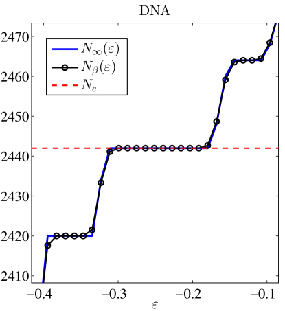
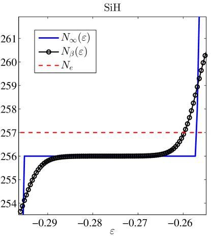
The integral in (17) can be evaluated numerically by sampling and at a number of quadrature points and performing a weighted sum of for . The evaluations of can be performed simultaneously using the factorization-based inertia counting procedure described above, with groups of processors. Since the derivative of the Fermi-Dirac function is sharply peaked, we can approximate in a given interval by sampling in a slightly wider interval. Fig. 1 shows the number of electrons at zero temperature obtained from inertia counting procedure, and the interpolated finite temperature profile at K for a DNA system (with finite gap) and a SiH system (with zero gap) near the Fermi energy. While the finite temperature smearing effect is negligible for insulators at K, it is more pronounced for metals and leads to a more smooth which is suitable for applying Newton’s method to find the chemical potential. On the other hand, the inertia counting procedure obtains the global profile of the cumulative density of states, and does not suffer from the problem of being trapped in intermediate band gaps.
This approximation to the function is then available for use in determining the approximate placement of the true by simple root finding: . In practice, we need to start from an interval which is large enough to contain the chemical potential. For systems with a gap the interval should also contain the gap edges. In this case, two roots are sought: and , where is small, say 0.1, and so and will be estimates of the band edges from which can be determined as .
The fidelity of , and thus the quality of the estimation of , depends on the density with which the interval can be sampled, which with a fixed number of sampling points for will increase as the interval is narrowed. In practice, the above procedure is repeated with progressively smaller intervals until either the estimate stabilizes or the size of the interval is small enough. Unless the original interval is very large, 2 or 3 inertia counts are enough to provide an adequate from which to start the PEXSI process, and the number of inertia counts can be one or even zero (i.e. the inertia counting procedure is turned off) in subsequent SCF iterations. Newton’s method in the solver then takes over for the final refining of .
The hybrid procedure of inertia counting and Newton’s method is efficient and robust for both insulating and metallic systems. This will be further demonstrated in section III.
II.4 Calculation of density of states and localized density of states
The density of states is defined as
| (18) |
The factor of two comes from spin degeneracy. As advanced in the previous section, the cumulative density of states (CDOS)
| (19) |
is exactly the function discussed there. To evaluate , we sample at a set of using the inertia counting procedure, and use an appropriate interpolation scheme to approximate for other values of . The approximation to the DOS is then obtained by numerical differentiation. We remark that inertia counting is not the only diagonalization-free method for computing the DOS. Other methods that make use of matrix vector multiplications only are also possible (see e.g.a recent review Lin et al. (2013b)).
Another physical quantity that can be easily approximated via selected inversion is the localized density of states (LDOS), defined as
| (20) |
and representing in fact the contribution to the charge density of the states with eigenvalues in the vicinity of , as filtered by the function.
When a finite basis set is used, the LDOS can be represented as
| (21) |
where is a matrix of the coefficients of the expansion in of the orbitals , and is a diagonal matrix of the eigenvalues. It follows from the Sokhotski-Plemelj formula Plemelj and Radok (1964)
| (22) |
that
| (23) |
where symbol in (22) stands for the Cauchy principal value.
Combining Eq. (21) and (23), we obtain the following alternative expression for the LDOS:
| (24) |
Note that Eq. (24) allows us to compute the LDOS without using any eigenvalue or eigenvector. In practice, we take to be a small positive number, and the local DOS can be approximated by
| (25) |
which is similar to the computation of the electron density. Again only the selected elements of the matrix are needed for the computation of the LDOS for each , and the selected elements can be obtained efficiently by the PSelInv procedure.
II.5 Interface to SIESTA and heuristics for enhancing the efficiency
SIESTA is a density functional theory code which uses finite-range atomic orbitals to discretize the Kohn-Sham problem Soler et al. (2002), and thus handles internally sparse H, S, and single-particle density matrices. SIESTA is therefore well suited to implement the PEXSI method along the lines explained above.
The PEXSI method can be directly integrated into SIESTA as a new kind of electronic-structure solver. Conceptually, the interface between SIESTA and PEXSI is straightforward. The existing SIESTA framework takes care of setting up the basis set and of constructing the sparse and matrices at each iteration of the self-consistent-field (SCF) cycle. and are passed to the PEXSI module, which returns the density matrix and, optionally, the energy-density matrix (needed for the calculation of forces) and the matrix that can be used to estimate the electronic entropy. SIESTA then computes the charge density to generate a new Hamiltonian to continue the cycle, until convergence is achieved. Energies and forces are computed as needed.
The details of the interface are controlled by a number of parameters which provide flexibility to the user, especially in regard to the bracketing and tolerances involved in the determination of the chemical potential, and in the context of parallel computation. We list some of the more relevant parameters in Table 1, but we should note that even finer control is possible by other, more specialized parameters.
| parameter | purpose |
|---|---|
| Initial guess of the lower and upper bounds of the chemical potential | |
| The number of SCF steps in which inertial count is used to narrow down the interval in which lies. | |
| Tolerance on number of electrons | |
| Electronic temperature | |
| Number of poles | |
| Number of processors used per pole | |
| The number of processors used for non-PEXSI operations |
The initial interval should be large enough to contain the true chemical potential. If it does not, the code will automatically expand it until is properly bracketed, but it is obviously more efficient to start the process with an appropriate interval, even if it is relatively large, and use the program’s refining features without the need for backtracking. Note that, due to the implicit reference energy used by SIESTA, is typically negative and within a Rydberg of zero, so the specification of should not be a problem in practice even when nothing is known about the electronic structure of the system. In fact the program can choose an appropriately wide starting interval if the user does not indicate one.
The bracketing interval can be refined by the use of the inertia counting procedure detailed in II.3. This is particularly important in the first few SCF steps in which the approximate electron density (and consequently the Hamiltonian) is far from converged. The parameter controls directly the number of SCF steps for which this procedure is followed. Beyond those, the PEXSI solver is directly invoked without further refinement. There is also the possibility of linking the use of inertia counting refinement to the convergence level of the calculation.
Because the chemical potential tends to oscillate in the first few SCF steps, a completely robust method should, in principle, search for a bracket afresh at every step, starting from a sufficiently wide interval. However, it is wasteful to completely ignore the previous bracketing when the SCF cycle reaches a more stable region, so we developed a heuristic to allow SIESTA-PEXSI to reuse the bracket determined in the previous SCF step, under various conditions related to the convergence level and to whether or not inertia counting is still used as a safeguard. We set the search interval for a new SCF step to be slightly larger (by a value that can also be controlled) than the final interval used in the previous SCF step. For some systems, an estimation of the change in the band-structure energy caused by the change in can be used to shift the bracket across iterations. If ever falls out of the bracketing interval, the algorithm recovers automatically by expanding the interval appropriately.
When the search interval is deemed appropriate, we invoke the PEXSI solver with a starting equal to the mid-point of the interval, and use the solver’s built-in Newton’s method to refine until the error in the total number of electrons is below .
The tolerance in the computed number of electrons is a key parameter of the PEXSI module, and it should be set to an appropriately small value to guarantee the necessary accuracy in the results. But there is no advantage to setting the tolerance too low in the early stages of the SCF cycle. Hence, the favored mode of operation of SIESTA-PEXSI is to use an on-the-fly tolerance level which ranges from a coarse value at the start and progressively (in tandem with the reduction of a typical convergence-level metric, which can also control the coarseness of the bracketing) decreases towards the desired fine level . Typically, no more than PEXSI solver iterations are needed to achieve a high accuracy in , and in practice the use of an adaptive tolerance level with proper bracketing means that just one or at most two solver iterations are enough for most of the steps in a complete SCF cycle. For gapped systems, with the starting well into the gap, the solver iteration can be turned off without affecting the accuracy of the results, leading to significant savings.
The total cost of a SCF cycle includes the factorizations required in the inertia counting bracket refinements, in addition to the cost of the PEXSI solver. As the cost of an inertia counting invocation is typically much lower than a solver iteration, it is clear that a strategy that uses at least a few inertia counting steps to properly bracket before invoking the solver will be in fact cheaper than one which incurs the extra costs associated with a bad guess of . The overall cost of the algorithm would depend on the uniformity of the convergence to self-consistency and on the electronic structure of the system (i.e, whether or not it has a gap). We will report the actual cost of search for a variety of systems in the next section.
The design of SIESTA-PEXSI provides some flexibility to users in terms of the usage of computational resources. If the user’s goal is a low time-to-solution on a large machine, the number of processors per pole ppp should be increased as much as possible. The overall number of processors Np should be set to ppp, where is the number of poles, to achieve complete parallelization over poles. If the goal is to minimize the number of processors involved in the computation, then should be set to the minimum number that allows the problem to fit in memory. It should be noted that the memory requirements of the PEXSI approach are significantly lower than those of the diagonalization-based algorithm, as the relevant matrices are handled in their original sparse form, and not converted to dense form as in ScaLAPACK. As the parallel efficiency over the number of poles is nearly perfect, the total cost (timeNp) does not depend on the total number of processors used, so the minimum-cost strategy can be used with a useful range of machine sizes: from total parallelization over poles in medium-to-large machines, to serial calculation of poles in small machines.
The number of processors that can be profitably used by the PEXSI module is typically larger than the number of processors that the non-solver part of SIESTA needs (as it is itself very efficient, having been coded for essentially O(N) operation). Hence the non-solver operations in the SIESTA side use a subset of the processors available, specified by the parameter in Table 1. Appropriate logic is in place to orchestrate the data movement and control flow.
III Numerical results
In this section we report the performance and accuracy achieved by the massively parallel SIESTA-PEXSI method for computing the ground state energy and atomic forces of several systems. We also show some other capabilities of SIESTA-PEXSI that may be useful for characterizing the electronic properties of materials.
To demonstrate that SIESTA-PEXSI can handle different types of systems, we choose five different test problems for our numerical experiments, including insulating, semi-metallic, and metallic systems, and covering all the relevant dimensions. Table 2 gives a brief description of each system.
Our calculations were performed on the Edison system at the National Energy Research Scientific Computing (NERSC) center. Each node consists of two twelve-core Intel “Ivy Bridge” 2.4-GHz processors and has 64 gigabytes (GB) of DDR3 1866-MHz memory.
| Name | type | Description |
|---|---|---|
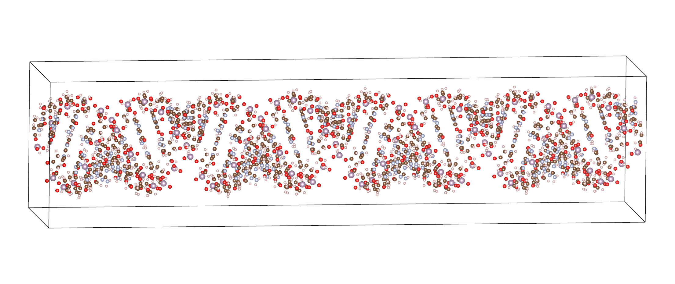
| DNA | 1D insulating | DNA. The basic unit (715 atoms) contains two base pairs of an A-DNA double helix. Replicating this unit along the axis of rotation results in several instances of this problem of different sizes, with quasi-one-dimensional character. The largest instance considered contains 25 units and is 76 nanometers long. |
| C-BN | 2D semi-metallic | A layer of boron nitride (BN) on top of a graphene sheet. Several instances of this problem are generated by varying the orientation of the BN sheet relative to the graphene layer within an appropriate periodic cell. The largest example considered of this quasi-two-dimensional system has 12700 atoms. |
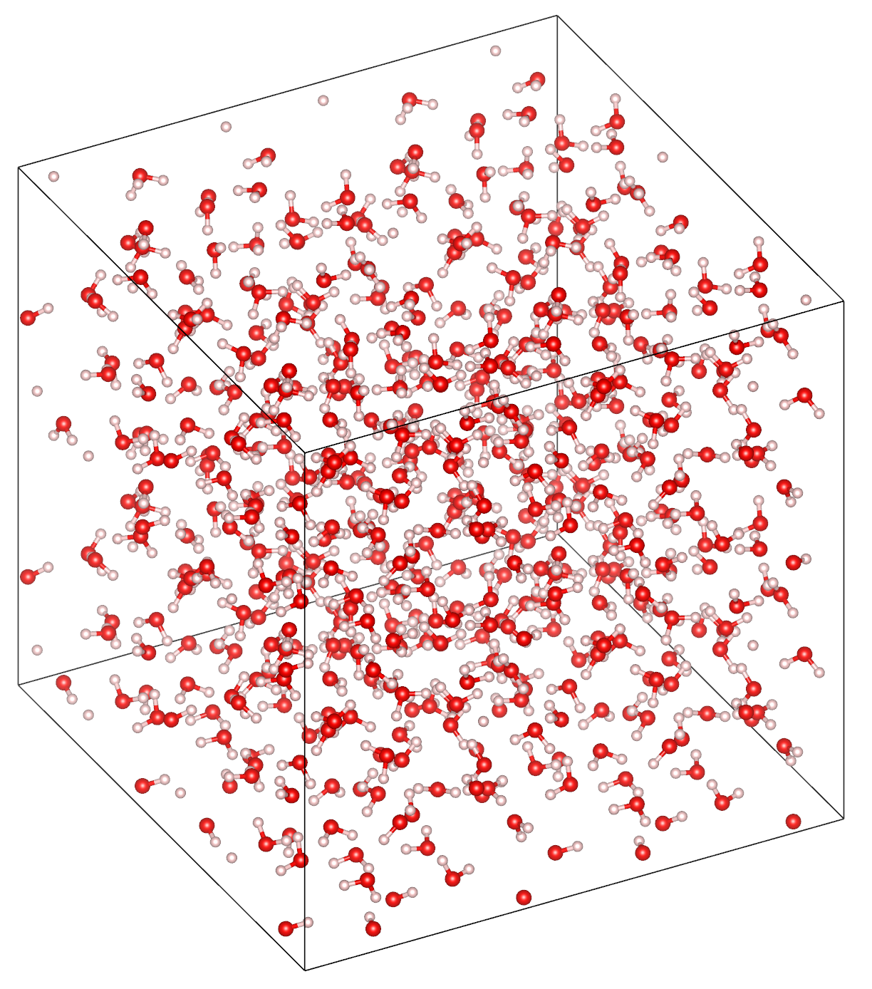
| H2O | 3D insulating | Liquid water. The basic repeating unit contains 64 molecules, and is generated by taking a snapshot of a molecular-dynamics run with the TIP4P force field. Appropriate supercells can be generated, with the largest having 8000 molecules, or 24000 atoms. |
| Al | 3D metallic | A bulk Al system generated from a supercell of the primitive unit cell. The positions of the atoms are perturbed by small random displacements to break the symmetry. This is a typical metallic system. |
| SiH | 3D, special | A bulk Si system with 64 atoms, with an H interstitial impurity. The Fermi level in this system is pinned by the position of an H-derived level within the gap. |
The number of atoms in the various instances of the problems listed on Table 2, the sizes of unit cells, as well as the matrix sizes and the sparsity (i.e., the percentage of nonzero elements) of the corresponding matrices and their and factors are given in Table 3. Note that the number of nonzero elements in is the same as the number of nonzero elements in if an equivalent factorization is to be used. We use DNA- to denote a DNA strand with unit cells, C-BNα to denote C-BN layers in which the Boron-Nitride layer is rotated by degrees relative to the graphene sheet (for this set of systems a lower implies a larger system size), and H2O- to denote a box of liquid water with unit cells. The various instances of DNA, C-BN, and H2O are used to test the performance (including parallel scaling) and accuracy of SIESTA-PEXSI, while the smaller Al and SiH systems are used mainly to showcase the accuracy of SIESTA-PEXSI and the effectiveness of the hybrid inertia counting plus Newton’s method for finding the correct chemical potential for metallic systems.
In all cases we use a DZP basis set, which results in 13 orbitals per atom for C, N, B, O, and P, and 5 orbitals per H atom.
| Example | Atoms | (nm) | |||
| DNA-1 | 715 | 7183 | 6.8% | 23% | 3.1 |
| DNA-4 | 2860 | 28732 | 1.7% | 6.2% | 12 |
| DNA-9 | 6435 | 64647 | 0.75% | 2.9% | 28 |
| DNA-16 | 11440 | 114928 | 0.42% | 1.7% | 49 |
| DNA-25 | 17875 | 179575 | 0.27% | 1.1% | 76 |
| C-BN2.3 | 1988 | 25844 | 5.9% | 36% | 5.5 |
| C-BN1.43 | 3874 | 50362 | 3.0% | 24% | 7.7 |
| C-BN0.57 | 7988 | 103844 | 1.5% | 15% | 11 |
| C-BN0.00 | 12770 | 166010 | 0.91% | 11% | 14 |
| H2O-8 | 1536 | 11776 | 2.3% | 28% | 2.5 |
| H2O-27 | 5184 | 39744 | 0.69% | 18% | 3.7 |
| H2O-64 | 12288 | 94208 | 0.29% | 12% | 5.0 |
| H2O-125 | 24000 | 184000 | 0.15% | 8.4% | 6.2 |
| Al | 512 | 6656 | 36% | 94% | 1.6 |
| SiH | 65 | 833 | 74% | 97% | 1.1 |
III.1 Accuracy of the SIESTA-PEXSI approach
We now report the accuracy of SIESTA-PEXSI in terms of the computed energies and atomic forces. We measure the accuracy of the energy by examining the difference between the free energy computed by SIESTA-PEXSI and that computed by the standard SIESTA approach in which free energies are obtained from density matrices constructed from the eigenvectors of . A similar metric is used for assessing the accuracy of atomic forces. We denote by the maximum force difference among all atoms.
In Table 4 we list the differences of energy per atom and force for fully converged calculations for a number of test problems with indication of the number of poles used in the pole expansion and of the target tolerance for electron count used in the chemical potential search. In all our tests we set the electronic temperature to 300K. As we can see from this table, the errors in the energy computed by SIESTA-PEXSI are typically of the order of eV per atom. The maximum error in atomic forces is of the order of eV/Å. Both are sufficiently small for most applications, and can be achieved with a modest number of poles and reasonable accuracy tolerance on . For SiH, and bring the error in the energy per atom to the level. In this more delicate case, one needs the extra accuracy to locate precisely the Fermi level, which is pinned in a gap state.
| System | (eV/atom) | (eV/Å) | ||
|---|---|---|---|---|
| DNA-1 | 50 | |||
| C-BN2.3 | 40 | |||
| H2O-8 | 40 | |||
| Al | 40 | |||
| SiH | 40 | 7 | ||
| SiH | 60 |
III.2 Efficiency of the SIESTA-PEXSI approach
We now report the performance of SIESTA-PEXSI in comparison to that of the standard SIESTA approach in which density matrices are obtained from the eigenvectors of computed by the ScaLAPACK diagonalization procedure based on the suite of subroutines pdpotrf, pdsyngst, pdsyevd/pdsyevx, and pdtrsm for transformation to a standard eigenvalue problem, solution, and back transformation, respectively.
We use instances of the DNA, C-BN and H2O problems to test both the strong scaling of the solver, which is measured by the change in wallclock time as a function of the number of processors used to solve a problem of fixed size, and the weak scaling, which is measured by the change of wall clock time as we increase in tandem both the problem size and the number of processors used in the computation.
Our timing measurements refer to a single SCF step. For completeness they include also the time used to setup the Hamiltonian and the overlap matrices, but this is in any case a very small fraction of the total () for these systems. The symbolic factorization is inexpensive compared to numerical factorization and selected inversion, and can be computed once for the entire SCF iteration using only the sparsity structure of and , and the time for symbolic factorization is excluded in the timings. It should be noted that the data for the diagonalization-based method include the time involved in constructing the density and energy-density matrices from the eigenvectors, needed at each SCF step.
The cost of the diagonalization method is determined directly by and and the internal, basically hardwired operating parameters in ScaLAPACK. The chemical potential is computed from the list of eigenvalues. In contrast, SIESTA-PEXSI determines the chemical potential iteratively in each SCF step, and thus the computational load depends on the actual sequence of bracketing and refining of followed. In order to provide an appropriate reference with which to compare the diagonalization-based results, our SIESTA-PEXSI timings include one (H2O) or two (DNA and C-BN) inertia counting cycles to narrow down the search interval for the chemical potential and one call of the PEXSI solver.
As mentioned above, one or two calls of the PEXSI solver are typically needed for an appropriately precise computation of as the SCF cycle unfolds. Given a good strategy for keeping a tight bracketing of , the final steps in the cycle close to convergence are likely to need just one call, and the same behavior is expected for most of the cycle when a good guess of the starting electronic structure can be provided, as in molecular-dynamics or geometry-optimization simulation. It should also be noted that later steps in the SCF cycle will not need the inertia counting procedure. Our timings for SIESTA-PEXSI are thus representative on average of the computational effort expected for a given system. In some cases, the actual effort will be higher by a small factor, and in others (as in systems with a gap) might even be smaller.
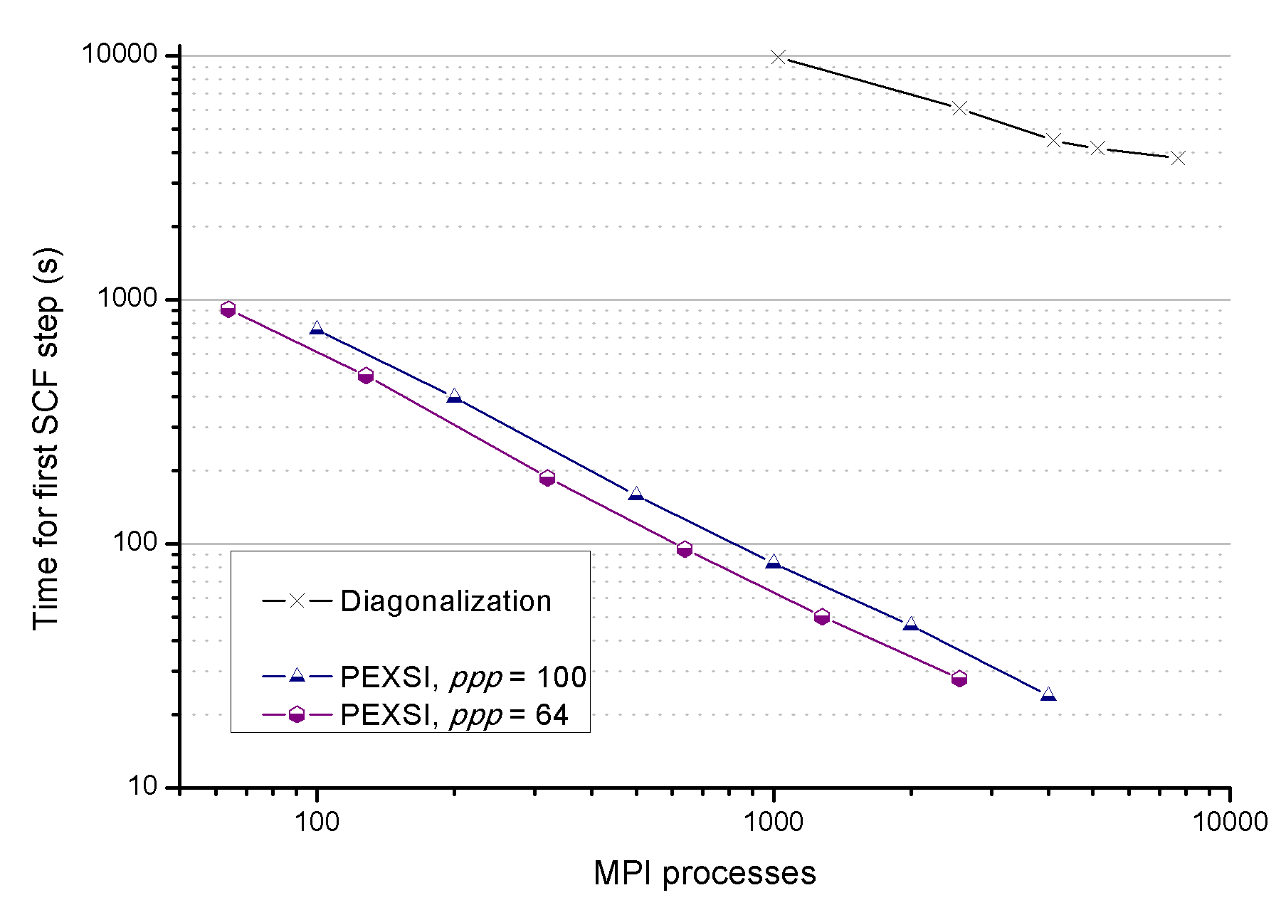
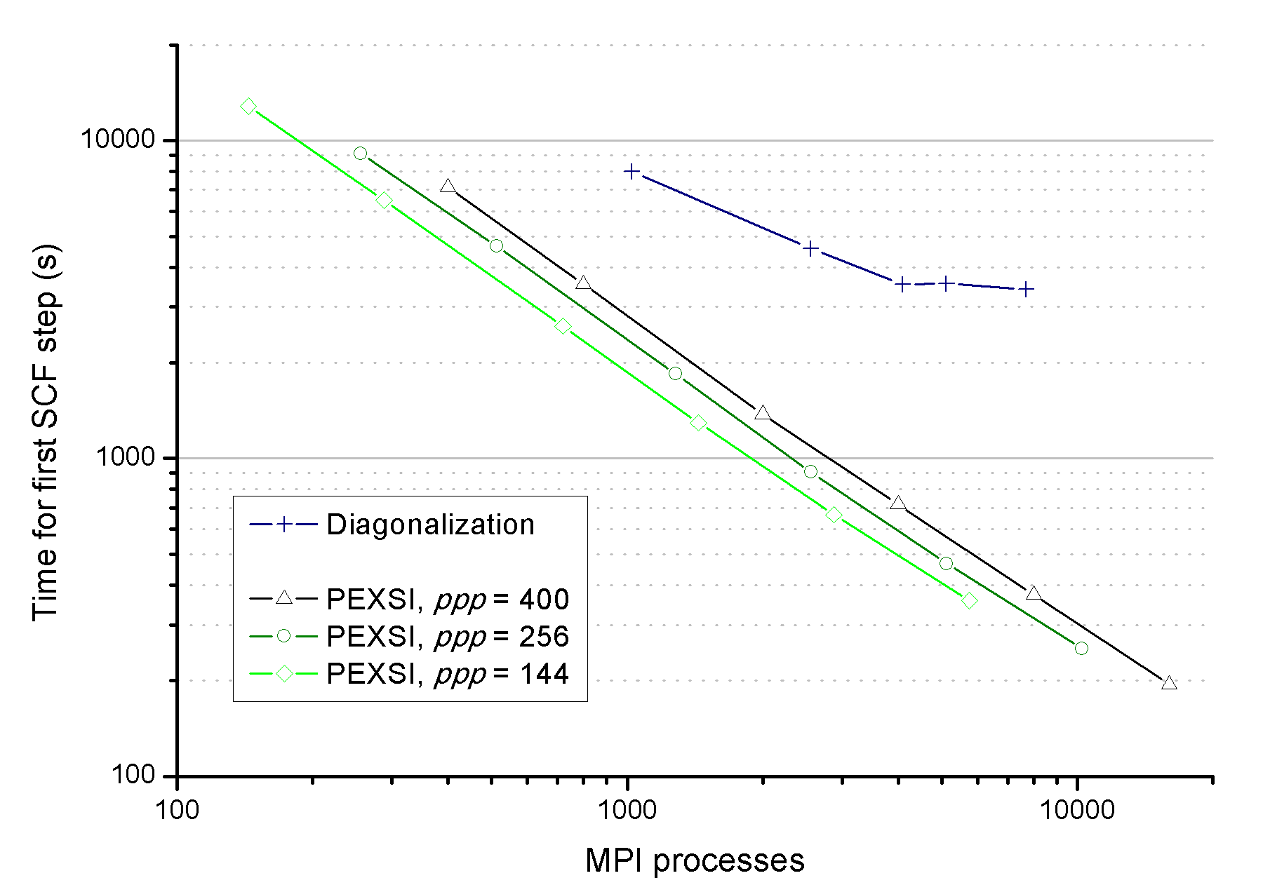
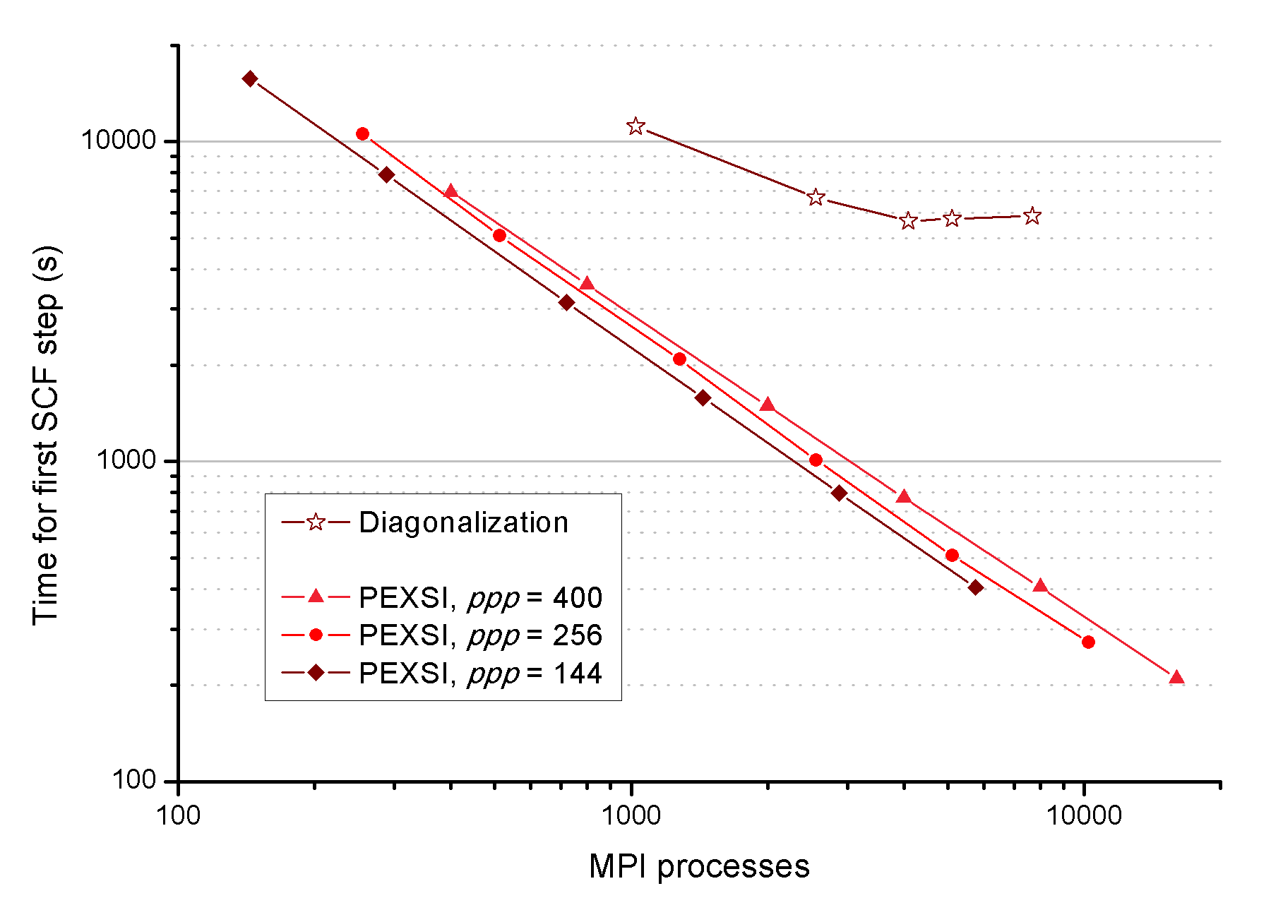
In Fig. 3, we plot the wallclock time required to complete the first SCF step as a function of the total number of processors used, for both SIESTA-PEXSI and the standard diagonalization method in SIESTA, when they are used to solve the DNA-25, C-BN0.00, and H2O-125 problems. In our experiments we used poles in the pole expansion approximation of the Fermi-Dirac function and varying degrees of concurrency over poles: , where . When , we simply loop serially over poles and perform parallel selected inversion on processors at each pole. When , full concurrency is achieved. For each test problem we connect all measurements that correspond to the same with a line. The nearly perfect scaling exhibited by these lines reflects the embarrassingly parallel nature of pole expansion. The further reduction in the wallclock time upon increasing depends for a given system on its size and the degree of sparsity of the Cholesky factor (or in and factors in the factorization). We observe that increasing from 64 to 100 leads to additional reduction in wallclock time by a factor of 1.2 for the DNA-25 problem. The matrix of DNA is very sparse. The matrices of C-BN and H2O are less sparse, and more processors can be effectively used to reduce the wallclock time of selected inversion. We observe that increasing from 144 to 400 leads to an additional speedup of 1.8 for C-BN0.00, and of 2 for H2O-125.
In Fig. 3, we also plot the wallclock time used by the standard diagonalization-based procedure. The computational complexity of diagonalization does not depend on the sparsity of the and matrices but only on their size, which is similar for all three systems, and therefore the performance of the method on these problems is comparable. The diagonalization curves in Fig. 3 start at around 1000 processors because this is the minimum number that would allow these problems to fit in memory, as the dense form of and is needed by the algorithm. A reasonably good parallel scaling can be observed up to 4000 processors, but the performance degrades after that.
We can also see that when around 1000 processors are used in the computation, SIESTA-PEXSI is approximately one order of magnitude faster than the diagonalization method for the C-BN0.0 and H2O-125 problems, and approximately two orders of magnitude faster for the DNA-25 problem. The performance gap between SIESTA-PEXSI and diagonalization widens as the number of processors used in the computation increases. This is due to the relatively limited scalability of ScaLAPACK, and that PEXSI can more efficiently utilize a large number of cores thanks to the two-level parallelism.
Even though there is a clear advantage of SIESTA-PEXSI in being able to use large numbers of processors, we should point out that its smaller memory footprint means that it can operate also with relatively small numbers of processors. Thus on Edison we can solve the DNA-25 and C-BN0.00 problems by SIESTA-PEXSI with as few as 144 processors for C-BN0.00 and 64 processors for DNA-25. For the DNA-25 problem, running SIESTA-PEXSI on 64 processors is still more than four times faster than running the standard diagonalization procedure on 5120 processors.
To measure the weak scaling of SIESTA-PEXSI, and compare it with that of the diagonalization-based procedure, we ran both solvers on multiple instances of the DNA, C-BN and H2O systems with different sizes. We adjust the number of processors so that it is approximately proportional to the dimension of the and matrices, i.e., as the problem size increases, we use more processors to solve the larger problem. For diagonalization, the number of processes for each system size are chosen so that there are approximately 40-50 orbitals per processor. For PEXSI, in all weak scaling tests, we use poles and fully exploit the concurrency at the pole expansion level, i.e., the selected inversions associated with different poles are carried out simultaneously on different groups of processors, for all sizes. This means that the increase in processor count with problem size is achieved with progressively higher values.
In Table 5 we report the wallclock time used to complete the first SCF step, and use the for the smallest size in each DNA, C-BN and H2O series as the basis for measuring weak scaling. If we increase the number of processors by a factor of when the problem size is increased by a factor of , the ideal weak scaling factor (in terms of the wall clock time) is
for DNA problems due to the quasi-1D nature. The ideal weak scaling factors are and for C-BN and H2O systems, due to the quasi-2D and 3D nature of the systems, respectively. Table 5 shows the ideal time for the PEXSI runs computed using those ideal weak scaling factors for each instance , where is the wallclock time for the smallest instance in each series. The weak-scaling for diagonalization is close to the expected cubic scaling , and the corresponding ideal time is not shown for simplicity.
| Diagonalization | Siesta-PEXSI | ||||
| Example | Proc. | (s) | Proc. | (s) | (s) |
| DNA-1 | 128 | 7.1 | 360 | 3.8 | 3.8 |
| DNA-4 | 512 | 123 | 1000 | 6.8 | 5.5 |
| DNA-9 | 1280 | 606 | 1960 | 10.9 | 6.3 |
| DNA-16 | 2560 | 2005 | 2560 | 16.6 | 8.6 |
| DNA-25 | 4096 | 4118 | 4000 | 24.4 | 8.6 |
| C-BN2.3 | 720 | 96.5 | 1440 | 69.2 | 69.2 |
| C-BN1.43 | 1280 | 393 | 2560 | 136 | 105 |
| C-BN0.57 | 2560 | 1422 | 5680 | 188 | 140 |
| C-BN0.00 | 4096 | 3529 | 10240 | 248 | 157 |
| H2O-8 | 256 | 16.8 | 640 | 12.3 | 12.3 |
| H2O-27 | 720 | 272 | 2560 | 47.3 | 35.0 |
| H2O-64 | 2048 | 1375 | 5760 | 126 | 87.5 |
| H2O-125 | 4096 | 5641 | 10240 | 314 | 188 |
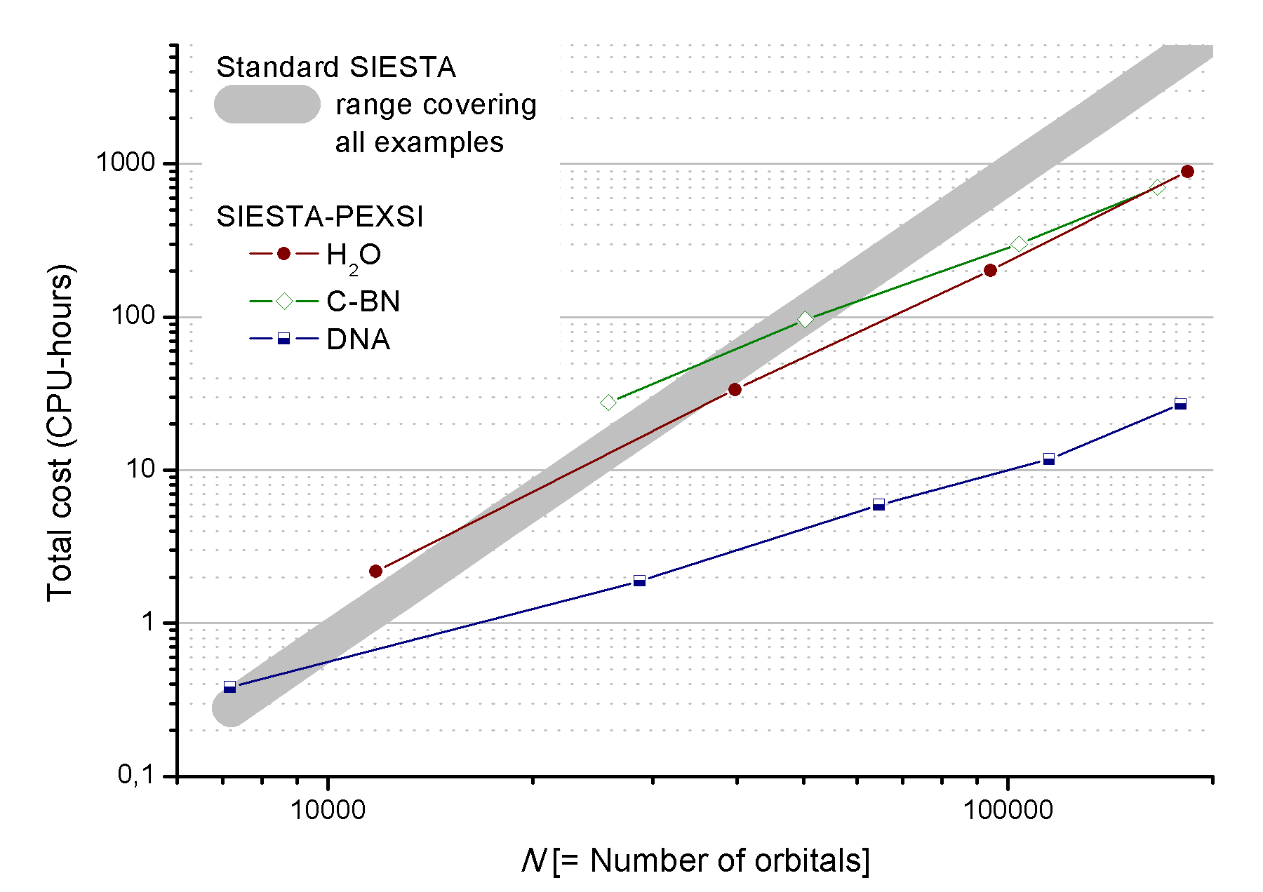
Another way to study the weak scaling of the SIESTA-PEXSI approach is to examine how the total computational cost, which is the product of the wallclock time and the number of processors (i.e., the first two columns for each method in Table 5), change with respect to the problem size. For perfect weak scaling, the change in cost should match that predicted by the computational complexity of the sequential algorithm. We plot the cost involved in solving each instance of the DNA, C-BN and H2O problems in Fig. 5, which shows that the data for each series falls approximately on a line. The (fitted) slope of the cost for DNA, which includes both factorization and selected inversion, is observed to be approximately 1.3, higher than the ideal scaling for quasi-1D systems. For C-BN the slope of the fitting line is approximately 1.7, which is a bit larger than the ideal scaling for quasi-2D systems. The slope of the line for the H2O series is approximately 2.18, again slightly larger than the expected scaling for 3D systems. The observed degradation in parallel scaling (relatively larger for DNA) comes about because neither selected inversion nor factorization (which has the same asymptotic complexity) can scale perfectly due to the complicated data communication and task dependency involved.
It should be noted also that the ideal weak-scaling data in Table 5 depends on the size and processor count chosen for the smallest instance of each series. We have already mentioned that all systems considered in our timings have been run with complete parallelization over poles. This limits the gains from increasing processor counts to the actual efficiency of selected-inversion and factorization within a pole, as a function of . Roughly, the computational load for a given instance will depend on the number of non-zeros in the Cholesky factor , which is plotted as a function of matrix size in Fig. 4. It can be seen that C-BN has the highest such non-zero density, closely followed by H2O. This is because C-BN has a more densely packed structure than H2O, and thus a larger prefactor, but there is a clear trend for a faster increase in the number of non-zeros in the Cholesky factor for H2O, in agreement with the asymptotic complexity of 3D and quasi-2D systems, respectively. The DNA system has significantly fewer non-zero values in L for a given size of H, and so it can use a relatively smaller number of processors per pole efficiently.
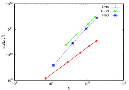
We can also see from Fig. 5 that the crossover point at which SIESTA-PEXSI becomes more efficient (in terms of cost) than the standard diagonalization procedure in SIESTA is around matrix dimension =7000 (700 atoms) for the DNA problem, =50,000 (4,000 atoms) for the C-BN problem and =40,000 (5,000 atoms) for the H2O problem. The actual orderings of the crossover points depend on the dimensionality (through the power of N in the scaling), and also on a prefactor which is system dependent.
Since more processors can be used efficiently, the advantage of SIESTA-PEXSI in time-to-solution performance is even more pronounced than the benefit from the reduction of total work load, and is already evident for smaller systems, as can be seen in Table 5.
The conclusions regarding the performance comparison between PEXSI and diagonalization, being based on the asymptotic scaling of the algorithm, remain largely valid even taking into account the efficiency improvements that can been obtained by refactoring some of the internals of ScaLAPACK Auckenthaler et al. (2011).
III.3 The search for chemical potential
As we discussed in section II.3, the current implementation of SIESTA-PEXSI uses a combination of an inertia counting bracketing technique and Newton’s method to determine the chemical potential that satisfies the nonlinear equation , where is defined in (13). In this section, we demonstrate the effectiveness of this approach for both metallic and insulating systems.
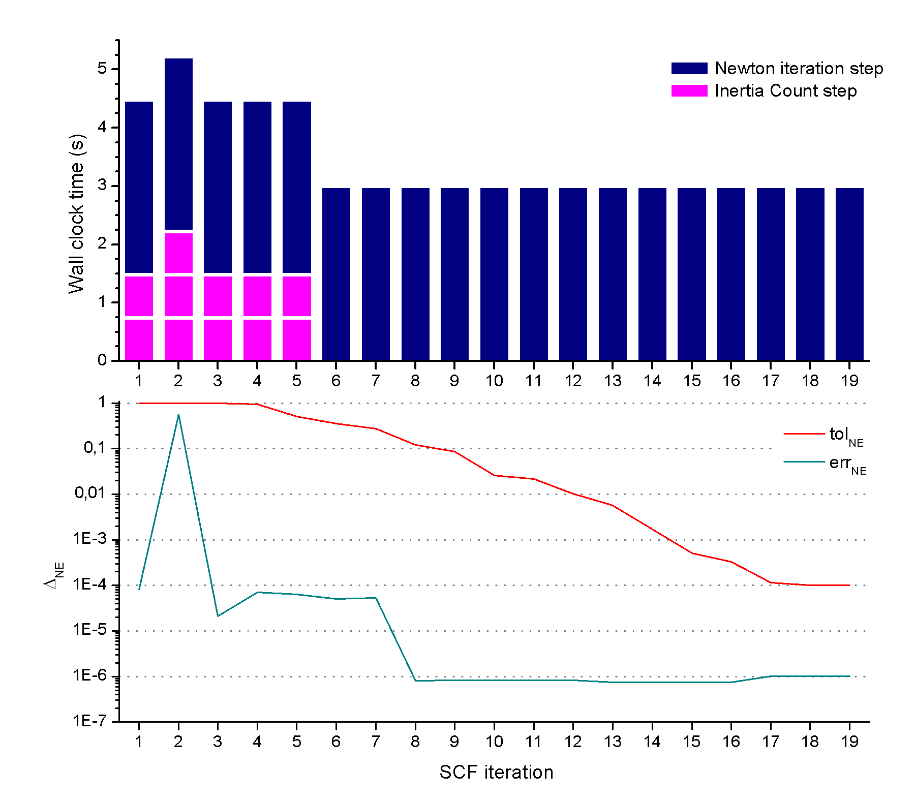
The metallic example is the SiH system with electrons. Since our calculation is spin-restricted, the odd number of electrons is solely controlled through the fractional occupation of the H-derived state in the gap. Any small perturbation of the chemical potential can change the number of electrons, and the perturbation is temperature dependent (we use 300 K). Despite the relatively small system size, this can be considered as the most difficult case for finding the chemical potential without having access to the eigenvalues. Fig. 6 illustrates the number of inertia counting cycles and PEXSI solver steps needed to obtain a chemical potential that satisfies for the converged SiH system when using 60 poles. The calculation starts from a wide initial search interval of eV, and uses an adaptive electron tolerance which starts at a coarse =0.1 and progressively tightens towards the target value of as the deviation from self-consistency in the H matrix elements moves towards its tolerance target of Ry. The number of inertia counting steps needed to narrow down the interval that contains the true chemical potential is roughly in the first few SCF steps. After the th iteration, the inertia counting procedure is turned off. The number of PEXSI solver steps needed is at most in the first few SCF steps, and it becomes 2 after the th SCF step. Fig. 6 also shows the absolute error at each SCF step, which is always below the set tolerance.
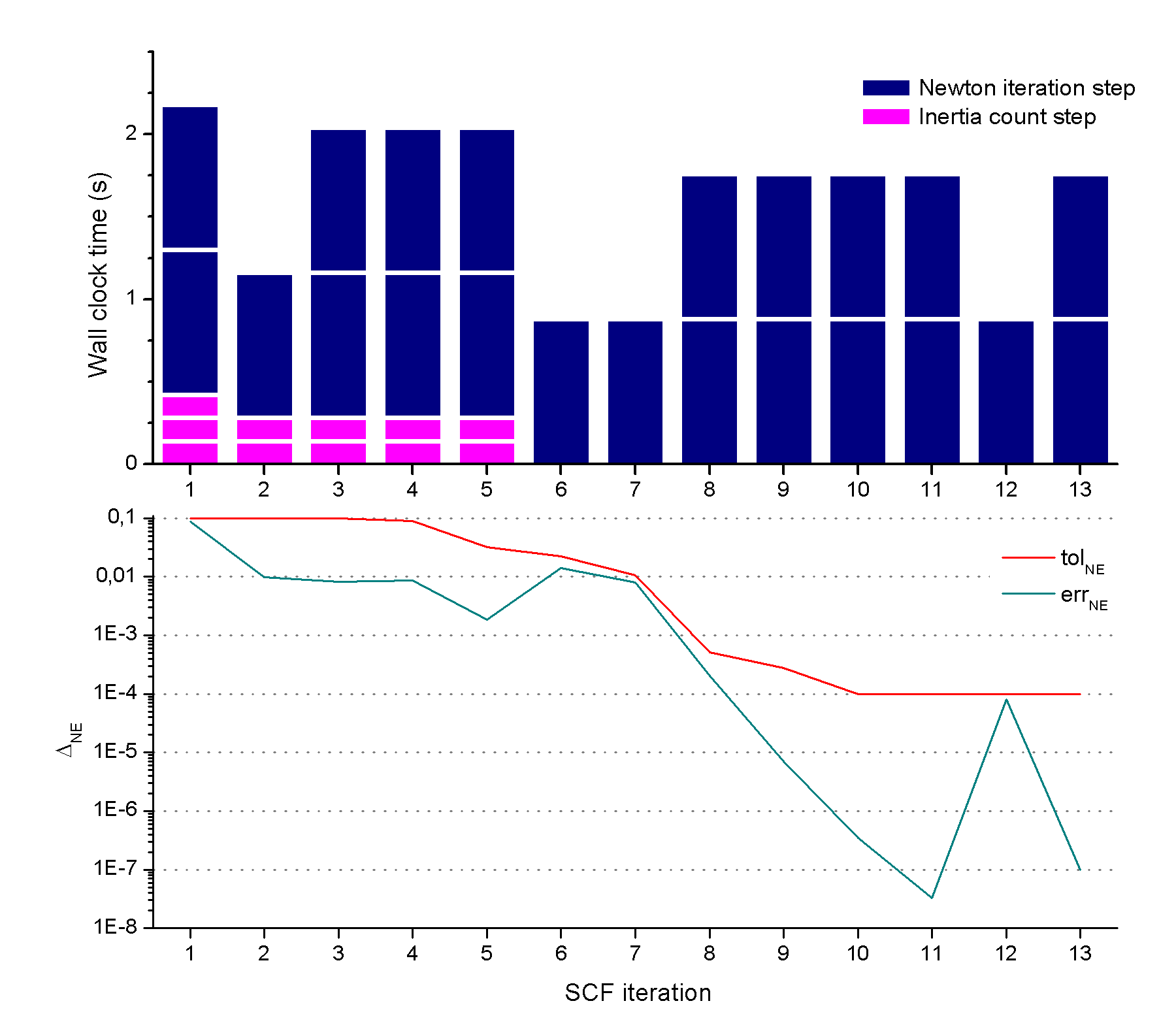
Our test for insulating systems is the DNA-1 system with electrons, at K and using 50 poles. Fig. 7 illustrates the number of inertia counting and PEXSI solver steps needed to reduce to a level below a final tolerance of , starting at a coarser tolerance of . The calculation also starts from a wide initial interval of eV. Usually two inertia counting steps are needed in the first few SCF iterations. The second iteration requires one more due to a large jump in H. After the th iteration, the inertia counting procedure is completely turned off. Throughout the SCF cycle, which ends when the deviation from self-consistency in H is below Ry, just one PEXSI solver call is needed to provide a solution with a number of electrons within the tolerance. This is because is kept within the gap by the bracketing procedure.
III.4 DOS and LDOS
In section II.4, we described how to use SIESTA-PEXSI to obtain spectral information of the atomistic system such as DOS and LDOS without computing eigenvalues and eigenvectors of . In Fig. 8 (a) we plot the DOS obtained from the standard diagonalization method and the inertia counting procedure implemented in SIESTA-PEXSI for the C-BN1.43 system near the Fermi level (“Ef”). We observe nearly perfect agreement between the DOS curves obtained from these two approaches. Fig. 8 (b) shows the DOS near the Fermi level for the DNA-25 system using both the inertia counting method and diagonalization. The usage of PEXSI for evaluating DOS without obtaining eigenvalues is also significant for systems at large size. For the DNA-25 system, using 64 and 3200 processors to evaluate points in the DOS near the Fermi energy (each group of 64 processors evaluate points of cumulative DOS with inertia counting) only takes sec, while diagonalization using the same number of processors takes sec. It should be noted that the performance of PEXSI can further be improved by simply using more cores: after the SCF converges, one can restart the calculation to compute the DOS using the converged density matrix, and use processors to compute points in the DOS in parallel. In such case, the wall clock can be reduced to sec.
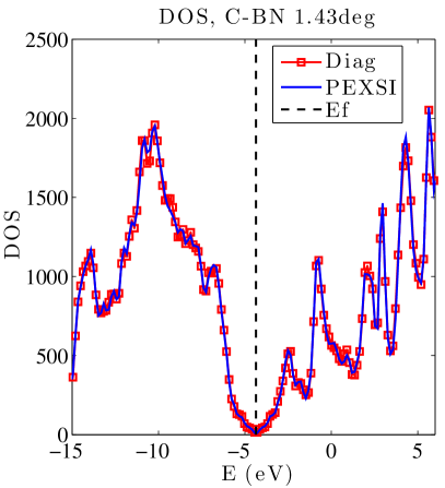
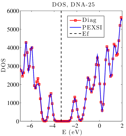
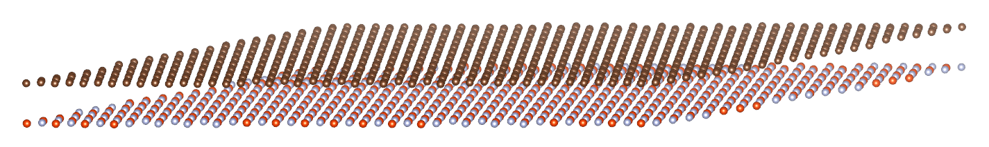
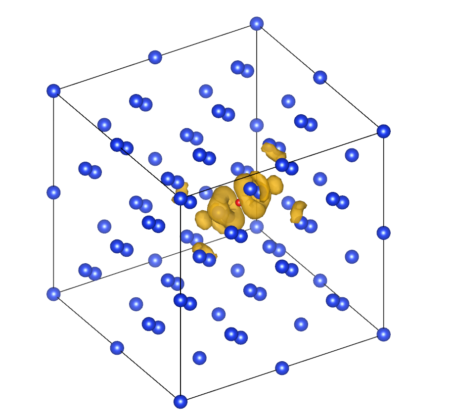
Fig. 9 presents the LDOS for the SiH system for an energy interval of width 0.4 eV around the Fermi level, showing the state due to the added H atom in the bulk Si system.
IV Conclusion
We have combined the pole expansion and selected inversion (PEXSI) technique with the SIESTA method for Kohn-Sham density functional theory (KDSFT) calculation. The resulting SIESTA-PEXSI method can efficiently use more than processors, and is particularly suitable for performing large scale ab initio materials simulation on high performance parallel computers. The SIESTA-PEXSI method does not compute eigenvalues or eigenvectors of the Kohn-Sham Hamiltonian, and its accuracy is fully comparable to that obtained from the standard matrix diagonalization based SIESTA calculation for general systems, including insulating, semi-metallic, and metallic systems at low temperature.
The current implementation of SIESTA-PEXSI does not yet support spin-polarized systems, but this can be achieved with minor changes to the code. Furthermore, the code does not support k-point sampling, as in principle it is not needed for large-enough systems. However, in some cases, as in graphene and similar semi-metallic systems, an appropriate computation of the spectral properties such as the DOS does need k-point sampling even when very large supercells are used. We will address this problem in future work, which requires modifying PEXSI to handle complex Hermitian matrices. In such case the shifted matrix is no longer symmetric but is only structurally symmetric. This further development will also be useful for ab initio study of non-collinear magnetism and spin-orbit coupling effects.
Acknowledgment
This work was partially supported by the Laboratory Directed Research and Development Program of Lawrence Berkeley National Laboratory under the U.S. Department of Energy contract number DE-AC02-05CH11231, by Scientific Discovery through Advanced Computing (SciDAC) program funded by U.S. Department of Energy, Office of Science, Advanced Scientific Computing Research and Basic Energy Sciences, by the Center for Applied Mathematics for Energy Research Applications (CAMERA), which is a partnership between Basic Energy Sciences and Advanced Scientific Computing Research at the U.S Department of Energy (L. L. and C. Y.), by the European Community’s Seventh Framework Programme [FP7/2007-2013] under the PRACE Project grant agreement number 283493 (G. H.), and by the Spanish MINECO through grants FIS2009-12721-C04-03, FIS2012-37549-C05-05 and CSD2007-00050 (A. G.).
References
- Bowler et al. (2002) D. R. Bowler, T. Miyazaki, and M. J. Gillan, J. Phys.: Condens. Matter 14, 2781 (2002).
- Fattebert and Bernholc (2000) J. L. Fattebert and J. Bernholc, Phys. Rev. B 62, 1713 (2000).
- Hine et al. (2009) N. D. Hine, P. D. Haynes, A. A. Mostofi, C. K. Skylaris, and M. C. Payne, Comput. Phys. Commun. 180, 1041 (2009).
- Yang (1991) W. Yang, Phys. Rev. Lett. 66, 1438 (1991).
- Li et al. (1993) X.-P. Li, R. W. Nunes, and D. Vanderbilt, Phys. Rev. B 47, 10891 (1993).
- McWeeny (1960) R. McWeeny, Rev. Mod. Phys. 32, 335 (1960).
- Goedecker (1999) S. Goedecker, Rev. Mod. Phys. 71, 1085 (1999).
- Bowler and Miyazaki (2012) D. R. Bowler and T. Miyazaki, Rep. Prog. Phys. 75, 036503 (2012).
- Kohn (1996) W. Kohn, Phys. Rev. Lett. 76, 3168 (1996).
- Prodan and Kohn (2005) E. Prodan and W. Kohn, Proc. Natl. Acad. Sci. 102, 11635 (2005).
- Lin et al. (2009a) L. Lin, J. Lu, L. Ying, and W. E, Chinese Ann. Math. 30B, 729 (2009a).
- Lin et al. (2009b) L. Lin, J. Lu, L. Ying, R. Car, and W. E, Comm. Math. Sci. 7, 755 (2009b).
- Lin et al. (2011) L. Lin, C. Yang, J. Meza, J. Lu, L. Ying, and W. E, ACM. Trans. Math. Software 37, 40 (2011).
- Lin et al. (2013a) L. Lin, M. Chen, C. Yang, and L. He, J. Phys. Condens. Matter 25, 295501 (2013a).
- Jacquelin et al. (2014) M. Jacquelin, L. Lin, and C. Yang, arXiv:1404.0447 (2014).
- Junquera et al. (2001) J. Junquera, O. Paz, D. Sanchez-Portal, and E. Artacho, Phys. Rev. B 64, 235111 (2001).
- Chen et al. (2010) M. Chen, G. C. Guo, and L. He, J. Phys.: Condens. Matter 22, 445501 (2010).
- Kenny et al. (2000) S. D. Kenny, A. P. Horsfield, and H. Fujitani, Phys. Rev. B 62, 4899 (2000).
- Ozaki (2003) T. Ozaki, Phys. Rev. B 67, 155108 (2003).
- Blum et al. (2009) V. Blum, R. Gehrke, F. Hanke, P. Havu, V. Havu, X. Ren, K. Reuter, and M. Scheffler, Comput. Phys. Commun. 180, 2175 (2009).
- Frisch et al. (1984) M. Frisch, J. Pople, and J. Binkley, J. Chem. Phys. 80, 3265 (1984).
- VandeVondele et al. (2005) J. VandeVondele, M. Krack, F. Mohamed, M. Parrinello, T. Chassaing, and J. Hutter, Comput. Phys. Commun. 167, 103 (2005).
- Chelikowsky et al. (1994) J. Chelikowsky, N. Troullier, and Y. Saad, Phys. Rev. Lett. 72, 1240 (1994).
- Tsuchida and Tsukada (1995) E. Tsuchida and M. Tsukada, Phys. Rev. B 52, 5573 (1995).
- Tsuchida and Tsukada (1998) E. Tsuchida and M. Tsukada, J. Phys. Soc. Jpn. 67, 3844 (1998).
- Lin et al. (2012) L. Lin, J. Lu, L. Ying, and W. E, J. Comput. Phys. 231, 2140 (2012).
- Becke (1993) A. D. Becke, J. Chem. Phys. 98, 5648 (1993).
- Adamo and Barone (1999) C. Adamo and V. Barone, J. Chem. Phys. 110, 6158 (1999).
- Soler et al. (2002) J. M. Soler, E. Artacho, J. D. Gale, A. García, J. Junquera, P. Ordejón, and D. Sánchez-Portal, J. Phys.: Condens. Matter 14, 2745 (2002).
- Artacho et al. (2008) E. Artacho, E. Anglada, O. Dieguez, J. D. Gale, A. García, J. Junquera, R. M. Martin, P. Ordejón, J. M. Pruneda, D. Sánchez-Portal, and J. M. Soler, J. Phys.: Condens. Matter 20 (2008).
- Goedecker (1993) S. Goedecker, Phys. Rev. B 48, 17573 (1993).
- Karypis and Kumar (1998) G. Karypis and V. Kumar, J. Parallel Distrib. Comput. 48, 71 (1998).
- Chevalier and Pellegrini (2008) C. Chevalier and F. Pellegrini, Parallel Comput. 34, 318 (2008).
- Li and Demmel (2003) X. Li and J. Demmel, ACM Trans. Math. Software 29, 110 (2003).
- Auckenthaler et al. (2011) T. Auckenthaler, V. Blum, H. J. Bungartz, T. Huckle, R. Johanni, L. Krämer, B. Lang, H. Lederer, and P. R. Willems, Parallel Comput. 37, 783 (2011).
- Sylvester (1852) J. J. Sylvester, Philos. Mag. 4, 138 (1852).
- Lin et al. (2013b) L. Lin, Y. Saad, and C. Yang, arXiv:1308.5467 (2013b).
- Plemelj and Radok (1964) J. Plemelj and J. R. M. Radok, Problems in the sense of Riemann and Klein (Interscience Publishers, New York, 1964).