Fleming-Viot particle system driven by a random walk on $\mathbb{N}$

Nevena Marić

University of Missouri - St. Louis

Abstract Random walk on ${\mathbb{N}}$ with negative drift and absorption at 0, when conditioned on survival, has uncountably many invariant measures (quasi-stationary distributions, qsd ) $\nu_{c}$. We study a Fleming-Viot(fv ) particle system driven by this process and show that mean normalized densities of the fv  unique stationary measure converge to the minimal qsd , $\nu_{0}$, as $N\to\infty$. Furthermore, every other qsd of the random walk ($\nu_{c}$, $c>0$) corresponds to a metastable state of the fv particle system.

Keywords

Quasi-stationary distributions. Fleming-Viot process. Selection principle. Metastability.

1 Introduction

In the Fleming-Viot (fv ) particle system there are $N$ ($N>1$) particles where each particle evolves as a Markov chain $Z_{t}$ which we call the driving process. The assumption is that $Z_{t}$ is irreducible on a countable state space and has an absorbing state. As soon as one particle is absorbed, it reappears immediately, choosing a new position according to the empirical measure at that time. Between the absorptions, the particles move independently of each other. Our focus is on the relation of empirical measures of the fv process with quasi-stationary distributions (qsds ) of the driving process.

A qsd is an invariant measure of the driving process conditioned to non-absorption. It is a non-trivial object whose existence and number are not completely investigated in countable spaces. Besides existence, explicit construction (simulation) of those measures is also a problem, especially if the probability of absorption is very small. One of the features of the present approach is that it provides numerical predictions. Using long-time simulations of the fv particle system, one can obtain immediate valuable insights about qsds of $Z_{t}$. An excellent overview of the achievements and challenges in the simulation of qsds is given in [9].

The Fleming-Viot approach to the study of qsds , in the discrete space setting, has been introduced in [14], [7]. Some questions have been answered for finite space [1] and countable space under certain conditions ([7],[3]), but there are still many open problems regarding limiting behaviour of the fv process. Here we examine perhaps the most paradigmatic and still puzzling case of a driving process being a nearest-neighbor random walk on ${\mathbb{N}}$, with absorption at origin. This random walk has infinitely many qsds if there is a drift towards 0, and none otherwise. In the former case it is a one parameter family $\nu_{c}$, where $0\leq c<1-p/q$ and $q,p$ are rates of hopping to the left and to the right respectively. We will refer to this particle system as FVRW (Fleming-Viot driven by a Random Walk). When $c=0$, the corresponding $\nu_{0}$ is called the minimal qsd . Under this measure, expected time till absorption is minimal, compared to the other qsds .

It has been recently proved in [3] that FVRW is ergodic. Since RW (Random Walk) has infinitely many qsds , the question is which one is approximated by the mean normalized densities of the FVRW stationary measure. It is believed ([14], [3], [10]) that in the limit, as $N\to\infty$, is exactly the minimal qsd : $\nu_{0}$. This property is usually reffered to as a selection principle. The analogous result is proven in the case of subcritical branching process [2], and some birth and death processes [16] but the methods used there do not apply in the RW case. We use graphical construction of the FVRW and computer simulations to support the above conjecture.

Here we also examine the role of others qsds , $\nu_{c}$ $(c>0)$ in the corresponding FVRW process. We performed simulations drawing starting profiles from a qsd that is not the minimal one (independently for each particle). For every combination of parameters $q$ and $c$ we observed significant sojourn time that increases exponentially both with $q$ and $c$. This feature is typical for metastability, which leads us to conjecture that each $\nu_{c}$ $(c>0)$ corresponds to a metastable state of the FVRW, as $N\to\infty$.

The remainder of the paper is organized as follows. Section 2 is devoted to the qsds of the random walk. In Section 3 we define the fv process and perform a graphical construction of FVRW. Section 4 contains findings based on simulations. Finally, Section 5 is reserved for a brief discussion.

2 Quasi-stationary distributions on countable spaces

Let $Z_{t}$ be a pure jump regular Markov process on a countable $\Lambda\cup\{0\}$ with absorbing state $0$. For $x,y\in\Lambda$ we will denote transition rates matrix $Q$ ($Q=(q(x,y)):q(x,y)$ is a transition rate from $x$ to $y$) and transition probabilities $P_{t}(x,y)$. Assume also that the exit rates are uniformly bounded above: $\bar{q}:=\sup_{x}\sum_{y\in\{0\}\cup\Lambda\setminus\{x\}}q(x,y)<\infty$, $P_{t}(x,y)>0$ for all $x,y\in\Lambda$ and $t>0$ and that the absorption time is almost surely finite for any initial state. This type of process is often seen in applications, for example if we consider the spread of an endemic infection, the number of infected individuals of the population could be $Z_{t}$. Classical Markov theory ensures that there is a unique stationary distribution concentrated at $0$. When the period before the absorption is extended (but a.s. finite), it is interesting to see whether the distribution of the number of infected individuals during this time exhibits a regular behavior.

Let $\mu$ be a probability on $\Lambda$. The law of the process at time $t$ starting with $\mu$ conditioned to non-absorption until time $t$ is given by

$$\varphi^{\mu}_{t}(x)=\frac{\sum_{y\in\Lambda}\mu(y)P_{t}(y,x)}{1-\sum_{y\in\Lambda}\mu(y)P_{t}(y,0)}\,.$$ (1)

A quasi stationary distribution (qsd ) is a probability measure $\nu$ on $\Lambda$ satisfying $\varphi^{\nu}_{t}=\nu$, that is: an invariant measure for the conditioned process. A qsd  is a left eigenvector $\nu$ for the restriction of the matrix $Q$ to $\Lambda$ with eigenvalue: $-\sum_{y\in\Lambda}\nu(y)q(y,0)$. That is, $\nu$ must satisfy the system

$$\sum_{y\in\Lambda}\nu(y)\,[q(y,x)+q(y,0)\nu(x)]=0,~{}~{}\forall x\in\Lambda.$$ (2)

(Recall $q(x,x)=-\sum_{y\in\Lambda\cup\{0\}\setminus\{x\}}q(x,y)$.)

So, finding a qsd involves solving a system of non-linear equations which is a difficult task, in general. However, in the case of the random walk that we consider here, we get a system of difference equations that is solvable using standard methods.

2.1 qsds for random walk on $\mathbb{N}$ with absorption at 0

Consider a continuous-time random walk on ${\mathbb{N}}$ with an absorbing barrier at 0: $q(x,x-1)=q$, $q(x,x+1)=p$, and $q(0,0)=0$. We will additionally assume that there is a drift towards 0, namely that $q>p$, since otherwise there is no a qsd [5].

A qsd for this process satisfies the equation (2):

$$\nu(x)=\frac{\nu(x-1)p+\nu(x+1)q}{p+q-\nu(1)q},~{}~{}x\geq 2.$$ (3)

Then we have homogeneous difference equations of the second order:

$$\nu(2)=\frac{1}{q}(p+q-\nu(1)q)\nu(1)$$

and

$$\nu(x)-\frac{(p+q-\nu(1)q)}{q}\nu(x-1)+\frac{p}{q}\nu(x-2)=0~{}~{}\mbox{for}~{}x\geq 3.$$

Define $c=[(\nu(1)-p/q-1)^{2}-4p/q]^{1/2}$. Then the characteristic equation

$$z^{2}-\frac{(p+q-\nu(1)q)}{q}z+\frac{p}{q}=0$$

has the following solutions

$$z_{1,2}=\frac{(p+q-\nu(1)q)/q\pm\sqrt{(p+q-\nu(1)q)^{2}/q^{2}-4p/q}}{2}=\frac{c\pm\sqrt{c^{2}+4p/q}}{2}$$

and the equation has real solutions for $(p+q-\nu(1)q)\geq 2\sqrt{pq}$ or $\nu(1)\leq(\sqrt{p/q}-1)^{2}$. Considering that $\nu(1)$ has also to be strictly positive, the last condition is equivalent to $0\leq c<|1-p/q|$. Recall that $p<q$, so the last condition is actually

$$0\leq c<1-p/q.$$ (4)

The minimal value $c=0$ would correspond to the minimal qsd . Then, $\nu_{0}(1)=(\sqrt{p/q}-1)^{2}$ and there is only one root of the above equation, $z=(p+q-\nu_{0}(1)q)/2q=\sqrt{\frac{p}{q}}$. In that case the solution has the form $\nu_{0}(n)=z^{n}(a+bn)$. The constants, found from $\nu_{0}(1)$ and $\nu_{0}(2)$, are

$a=0,b=(p+q)/\sqrt{pq}-2$ and the general solution is given by

$$\nu_{0}(n)=\Big{(}\frac{p+q}{\sqrt{pq}}-2\Big{)}n\Big{(}\sqrt{\frac{p}{q}}\Big{)}^{n}=\nu_{0}(1)n\Big{(}\frac{p/q+1-\nu_{0}(1)}{2}\Big{)}^{n-1}.$$

For $c>0$ we will obtain another solution for the system (3) which would also be a qsd . So there is an entire family of qsds parametrized by $c$, and they have the following form

$$\nu_{c}(n)=\frac{\nu_{c}(1)}{c}\Big{[}\Big{(}\frac{p/q+1-\nu_{c}(1)+c}{2}\Big{)}^{n}-\Big{(}\frac{p/q+1-\nu_{c}(1)-c}{2}\Big{)}^{n}\Big{]}.$$ (5)

Observe that as $c$ increases, $\nu_{c}(1)$ gets smaller which can also be seen in Figure 1

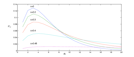
Figure 1: Quasi-stationary distributions for RW on ${\mathbb{N}}$ with $q=2/3,p=1/3$. They are parametrized by $c:0\leq c<0.5$

3 Fleming-Viot particle system driven by a Random Walk (FVRW)

The Fleming-Viot process (fv ). Consider a system of $N$ particles ($N\geq 2$) evolving on a countable space $\Lambda$. The particles move independently, each of them governed by the transition rates $Q$ until absorption. Since there cannot be two simultaneous jumps, at most one particle is absorbed at any given time. When a particle is absorbed to 0, it goes instantaneously to a site in $\Lambda$ chosen with the empirical distribution of the particles remaining in $\Lambda$. In other words, it chooses one of the other particles uniformly at random and jumps to its position. Between absorption times the particles move independently, governed by $Q$.

This process has been initially studied in a Brownian motion setting [4]. Countable space has been treated firstly in [14], [7] and later in [2], [1], [3]. The original process introduced by Fleming and Viot [8] is a model for a population with constant number of individuals which also encodes the positions of particles.

The generator of the fv process acts on functions $f:\Lambda^{(1,\dots,N)}\to{\mathbb{R}}$ as follows

$${\mathcal{L}}^{N}f(\xi)=\sum_{i=1}^{N}\sum_{y\in\Lambda\setminus\{\xi(i)\}}\Bigl{[}q(\xi(i),y)+q(\xi(i),0)\,\frac{\eta(\xi,y)}{N-1}\Bigr{]}(f(\xi^{i,y})-f(\xi)),$$ (6)

where $\xi^{i,y}(j)=y$ for $j=i$ and $\xi^{i,y}(j)=\xi(j)$ otherwise and

$$\eta(\xi,y):=\sum_{i=1}^{N}{\mathbf{1}}\{\xi(i)=y\}.$$

Namely, $\eta(\xi,y)$ is the number of particles at site $y$, in the configuration $\xi$. We call $\xi_{t}$ the process in $\Lambda^{(1,\dots,N)}$ with generator (6) and $\eta_{t}=\eta(\xi_{t},\cdot)$ the corresponding unlabeled process on $\{0,1,\dots\}^{\Lambda}$; $\eta_{t}(x)$ counts the number of $\xi$ particles in state $x$ at time $t$.

For $\mu$ a measure on $\Lambda$, we denote by $\xi^{N,\mu}_{t}$ the process starting with independent identically $\mu$-distributed random variables $(\xi^{N,\mu}_{0}(i),\,i=1,\dots,N)$; the corresponding variables $\eta^{N,\mu}_{0}(x)$ follow a multinomial law with parameters $N$ and $(\mu(x),\,x\in\Lambda)$.

3.1 Construction of FVRW process

Graphical representation in interacting particle systems has been used extensively since the pioneering work of Harris [11]. The main idea is to construct the process explicitly in terms of independent collections of Poisson processes [13]. Along these lines, here we perform a graphical representation/construction of the FVRW process $\xi_{t}^{N}$. Events in Poisson processes correspond to clocks according to which the particles jump, and we will call them internal times. When a clock goes off, random variables called marks are used to determine next position of the particle. For each $i=1,\dots,N$, we define independent stationary marked Poisson processes on ${\mathbb{R}}$:

• Internal times: Poisson process with rate $q+p$: $(b^{i}_{n})_{n\in{\mathbb{Z}}}$, with marks $((B^{i}_{n}(x),\,x\in\Lambda),\,n\in{\mathbb{Z}})$, $((C^{i}_{n}),\,n\in{\mathbb{Z}})$.

The marks are independent of the Poisson processes and mutually independent. Their marginal laws are given below:

• ${\mathbb{P}}(B^{i}_{n}(x)=x+1)=\frac{p}{p+q}$,
  ${\mathbb{P}}(B^{i}_{n}(x)=x-1)=\frac{q}{p+q}$, $x\in{\mathbb{N}}$.

• ${\mathbb{P}}(C^{i}_{n}=j)=\displaystyle{\frac{1}{N-1}}$, $j\neq i$.

Denote by $(\Omega,\mathcal{F},{\mathbb{P}})$ the probability space on which the marked Poisson processes have been constructed. Discard the null event corresponding to two simultaneous events at any given time.

We construct the process in an arbitrary time interval $[s,t]$. Given the mark configuration $\omega\in\Omega$ we construct $\xi_{[s,t]}^{N,\xi}(=\xi^{N,\xi}_{[s,t],\omega})$ in the time interval $[s,t]$ as a function of the Poisson times, and their respective marks, and the initial configuration $\xi$ at time $s$.

Construction of $\xi_{[s,t]}^{N,\xi}=\xi_{[s,t],\omega}^{N,\xi}$

Since for each particle $i$ there is a Poisson process, the number of events in the interval $[s,t]$ is Poisson with mean $N(p+q)$. So the events can be ordered from the earliest to the latest. If at time $s$ the initial configuration is $\xi$, then, we proceed event by event following the order as follows (between Poisson events the configuration does not change):
If at the internal time $b^{i}_{n}-$ the state of particle $i$ is $x$, and $x\neq 1$ then at time $b^{i}_{n}$ particle $i$ jumps to state $B^{i}_{n}(x)$ regardless of the position of the other particles. If $x=1$ and $B^{i}_{n}(1)=0$, particle $i$ jumps to the site where particle $C^{i}_{n}$ is; if $B^{i}_{n}(1)=2$, then the state of particle $i$ becomes 2. The configuration obtained after using all events is $\xi_{[s,t]}^{N,\xi}$.

The above graphical construction is algorithmized in the Algorithm FVRW:

3.2 Algorithm FVRW

• T=0; Sample $\xi_{0}(j)\sim\mu$, $j=1,...,N$;
  Set $\eta_{0}(x)=\sum_{i=1}^{N}{\mathbf{1}}\{\xi_{0}(i)=x\},x=1,2,...$
  

• Sample $t\sim Exponential(q+p)$.
  Choose particle $i$ uniformly at random from $\{1,...,N\}$.
  Number of particles at the site $\xi_{T}(i)$ is decreased by 1: $\eta_{T+t}(\xi_{T}(i))=\eta_{T}(\xi_{T}(i))-1$.
  

• Sample $U\sim Uniform(0,1)$.
  -If $U<q/(q+p)$

  • if $\xi_{T}(i)=1$ then choose particle $j$ uniformly at random from $\{1,...,i-1,i+1,...,N\}$.
    Particle $i$ jumps to the position of particle $j$: $\xi_{T+t}(i)=\xi_{T}(j)$ and number of particles at the site $\xi_{T}(j)$ increases by 1: $\eta_{T+t}(\xi_{T}(j))=\eta_{T}(\xi_{T}(j))+1.$

  • if $\xi_{T}(i)\neq 1$ then particle $i$ jumps one position to the left and the number of particles at the new site gets updated: $\xi_{T+t}(i)=\xi_{T}(i)-1$; $\eta_{T+t}(\xi_{T}(i)-1)=\eta_{T}(\xi_{T}(i)-1)+1$.

  -If $U>q/(q+p)$ (i.e. with probability p/p+q)
  then particle $i$ jumps one position to the right and the number of particles at the new site gets updated: $\xi_{T+t}(i)=\xi_{T}(i)+1$; $\eta_{T+t}(\xi_{T}(i)+1)=\eta_{T}(\xi_{T}(i)+1)+1$.
  

• $T\leftarrow T+t$. If $T<\tau$ go to Step 2; otherwise STOP.

  The output of the algorithm is $\xi^{N,\mu}_{[0,\tau]}$.

4 Findings and Conjectures

In this section we present the findings based on the simulations performed using MATLAB. Our focus is on getting an insight into qualitative rather than quantitative properties of the FVRW process. Let us define the mean normalized density as

$$\rho^{N,\mu}_{t}(k)={\mathbb{E}}\frac{\eta_{t}^{N,\mu}(k)}{N},~{}~{}k\in{\mathbb{N}}$$

where the initial position of all particles is chosen independently with distribution $\mu$. We will use further the notation ${\hat{\rho}^{N}_{t}}$ for the estimated density at time $t$ using a Monte Carlo method. It is obtained as an average, over 50 independent realizations of $\eta_{t}$, generated by the Algorithm FVRW.

4.1 Selection principle

It was conjectured in [14] that FVRW with $(q>p)$ is ergodic, a result which has been recently proved in [3]. Let $\rho^{N}=\rho^{N}_{\infty}$ be the density of the fv process in equilibrium (note that initial configuration does not play a role here so we omit it from the notation). It has been also conjectured in [14] that as $N$ goes to infinity this empirical equilibrium density approaches the minimal qsd .

Conjecture 1 ( Marić [14]).

For the fv driven by RW on ${\mathbb{N}}$, with $q>p$

$$\rho^{N}\to\nu_{0},~{}~{}N\to\infty$$

Heuristic arguments are based on the following two facts: 1. $\rho^{N,\mu}_{t}$ converges to $\varphi_{t}$ (defined in (1)) as $N\to\infty$ (Theorem 1.2 in  [7]). 2. $\varphi_{t}$ converges to the minimal qsd $\nu_{0}$, as $t\to\infty$ [6].

Analogous result was proven for the fv driven by a subcritical Galton-Watson [2] and very recently, for those driven by some birth and death processes (not including a random walk)[16] . In what follows we are going to provide simulation evidence in support of the above Conjecture.

Let ${\hat{\rho}^{N}}$ be the estimated limiting density profile, obtained as an average, over 50 independent realizations of $\eta_{t}$, obtained using the Algorithm FVRW. Initially all the particles are positioned at 5 and $t$ is chosen large enough that we may say the equilibrium distribution has been reached. The initial position is chosen to be 5 without any special reason, since the process is ergodic, initial configuration does not affect long-time behavior.

Figure 2 compares minimal qsd with the limiting FVRW densities for $N=100,500,10000$. Note how, with larger $N$, the approximation by $\nu_{0}$ becomes better.

Figure 2: Red curve is the minimal qsd $\nu_{0}$. Three other curves, obtained from simulations, present $\hat{\rho}^{N}$, for $N=100,500,50000$.

Let us define the L-truncated total variation distance between two probability measure $\mu$ and $\nu$ as $d_{TV}^{L}(\mu,\nu)=1/2\sum_{i=1}^{L}|\mu(i)-\nu(i)|$. The truncation is necessary since we are looking at the finite window of infinite-volume measures. Then we obtain ${\hat{\rho}^{N}}$ for different values of $N$ in the range $(500,1000,...,50000)$ and show the distance $d_{TV}^{L}({\hat{\rho}^{N}},\nu_{0})$, for $L=150$. Note that, when truncated at $L=150$, measure $\nu_{0}$, is still very well approximated. For example, for $q=2/3,p=1/3$, $\nu_{c}(100)\sim 10^{-14}$, and $\nu_{c}$ is decreasing in $n$ for $n>3$. Consequently, $d_{TV}^{150}({\hat{\rho}^{N}},\nu_{0})$ is very close to $d_{TV}({\hat{\rho}^{N}},\nu_{0})$, (non-truncated) total variation distance.

In Figure 3 are presented the obtained values for $q=2/3,p=1/3$. It clearly supports the conjecture that $d_{TV}({\hat{\rho}^{N}},\nu_{0})\to 0$ as $N\to\infty$.

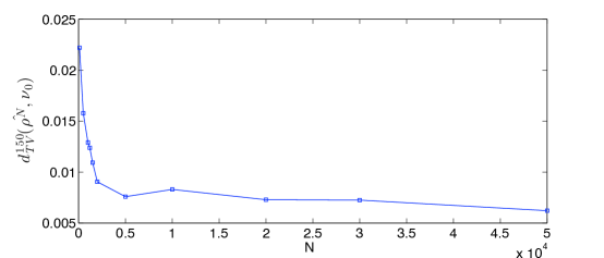
Figure 3: 150-truncated total variation distance between ${\hat{\rho}^{N}}$ and $\nu_{0}$ is approaching $0$ as $N$ gets larger. Here $q=2/3,p=1/3$.

4.2 Metastability

Since the minimal qsd is the limiting density of the FVRW process it is natural to ask whether there is a special meaning of other qsds for this particle system. What happens if initially each particle’s position is chosen according to another qsd (not the minimal one)?

Suppose then that initially each particle is positioned, independently of others, according to $\nu_{c}$ ($c>0$), where $\nu_{c}$ given by (5), is a qsd for the random walk on ${\mathbb{N}}$. Although $\nu_{c}$ is an infinite-volume measure, the number of particles $N$ is finite, and the entire system is therefore finite. The position of right-most particle changes, it can be very far from the origin, but at any given time it is finite.

Now, let $\hat{\rho}^{N,c}_{t}$ be the estimated mean density (via Monte Carlo) of the FVRW at time $t$. Let also $\hat{\rho}^{N,c}$ be the Monte Carlo estimated mean stationary (steady) state, which exists by the arguments mentioned at the beginning of this section. In order to monitor velocity of convergence we plot $d_{TV}({\hat{\rho}_{t}^{N,c}},{\hat{\rho}^{N,c}})$ as a function of $t$. Note that both ${\hat{\rho}_{t}^{N,c}}$ and $\hat{\rho}^{N,c}$ are finite-volume probability measures and there is no need here to use truncated total variation distance.

Figure 4 displays a typical result, where $N=50000,q=4/5,c=0.6$.

Remark: In all figures in this section where $x$-axis is labeled with $t$, the time is scaled. Real simulation time is 100 times larger.

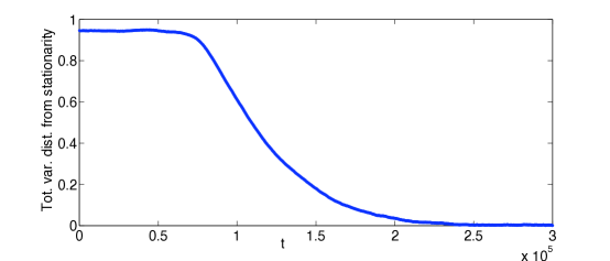
Figure 4: Total variation distance from the steady state $d_{TV}({\hat{\rho}_{t}^{N,c}},{\hat{\rho}^{N,c}})$ as a function of $t$. Here q=4/5; c=0.6; N=50000.

We have performed numerous simulations changing all three parameters ($q,c,N$). In each case that we analyzed, a plateau was present, meaning that the process stays a “long” time in the initial distribution. Then, it starts “rapidly” to approach the equilibrium. This type of behavior is typical for metastability ([12], [15]), as is the requirement that the plateau length be approximately an exponential function of a certain parameter of the system.

For any $q>1/2$, define the plateau length as

$$PL_{c,q}^{N}(\epsilon)=\min\{t:d_{TV}({\hat{\rho}_{t}^{N,c}},{\hat{\rho}^{N,c}_{0}})>\epsilon\}$$

where $\epsilon$ is positive but relatively small. Typically, we take $\epsilon=0.005$. In what follows, we compare $PL_{c,q}^{N}$ for different values of $N,c,q$ respectively. Each time, the other two parameters stay fixed.

$\bullet$ Plateau length as a function of $N$

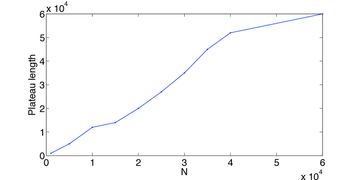
Figure 5: Plateau length $PL_{c,q}^{N}(0.005)$ as a function of number of particles N. Here $q=0.8,c=0.6$

As we can see on the Figure 5, growth in $PL_{c,q}^{N}$ with $N$ is observed but it is very slow, almost linear. It is somehow not surprising that with increase in $N$ there is no dramatic change in the behavior of the process. Having in mind arguments around the Selection principle we would expect that a qsd of the random walk $\nu_{c}$ has a special meaning (if any) for the FVRW process in the limit as $N\to\infty$.

$\bullet$ Plateau length as a function of $c$

As mentioned in the Section 2, for every choice of $q$ and $p$ ($q>p$), there is an entire family of qsds , parametrized by $c$ where $0\leq c<1-p/q$. In Figure 6 is displayed $d_{TV}({\hat{\rho}_{t}^{N,c}},{\hat{\rho}^{N,c}})$ for different values of c. Obviously plateau lengths increase with $c$.

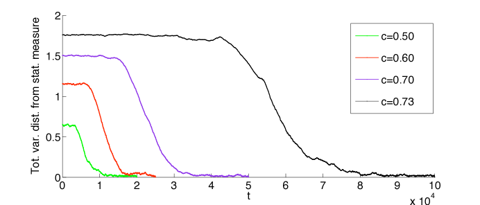
Figure 6: $d_{TV}({\hat{\rho}_{t}^{N,c}},{\hat{\rho}^{N,c}})$ for $c=0.5,0.6,0.7,0.73$. Here q=0.8, p=0.2; N=5000.

A more detailed comparison, showing $PL_{c,q}^{N}$ as a function of $c$, is given in Figure 7.

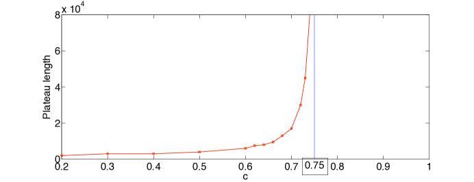
Figure 7: Plateau length $PL_{c,q}^{N}(0.005)$ for different values of c =0.2,…,0.73. Here q=0.8, p=0.2; N=5000. For q=0.8, p=0.2 the condition (4) gives a range for $c$: $0\leq c<0.75$.

From Figure 7 it is clear that the length of the plateau increases significantly with $c$ and appears to diverge as $c\to 0.75$. For the particular choice of parameters $q=0.8,p=0.2$, value 0.75 corresponds to the theoretical bound for $c$ as given in condition (4).

At the same time, as $c$ increases, $\nu_{c}$ becomes more “flat” with heavier tails (see Figure 1). One could think then that the main feature affecting plateau lengths is “flatness” of the initial profile. For that reason we performed simulations using as initial distribution the uniform distribution over large interval $[0,100]$. This initial profile, of course, does not correspond to any $\nu_{c}$. It may be clearly seen in Figure 8, that in this case convergence is very fast and no plateau is observed whatsoever.

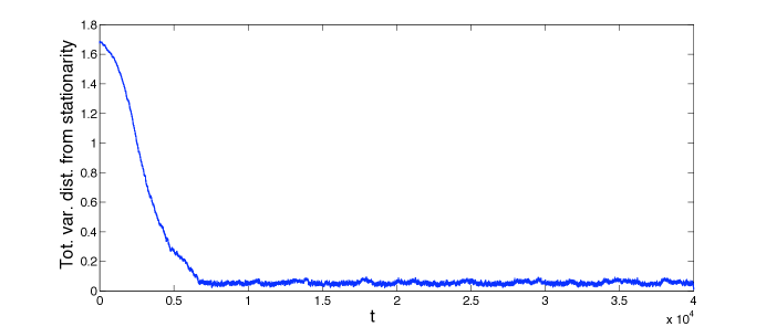
Figure 8: $d_{TV}({\hat{\rho}_{t}^{N,\mu}},{\hat{\rho}^{N,\mu}})$ as a function of $t$, where $\mu$ is a uniform distribution on [1,100]; Here N=1000; q=2/3; p=1/3. No plateau.

$\bullet$ Plateau length as a function of $q$

Lastly, we compare sojourn times (plateau lengths) as a function of the rate $q$ (actually the ratio $q/p$, but in our simulations it is taken $p=1-q$). We approximate plateau lengths for different values of $q$ and fixed value of $c=0.1$. From condition (4) we know that the minimum value of $q$ that allows $\nu_{0.1}$ is $q=0.5263$. The results are shown graphically in Figure 9. The log-log plot is shown in Figure 10.

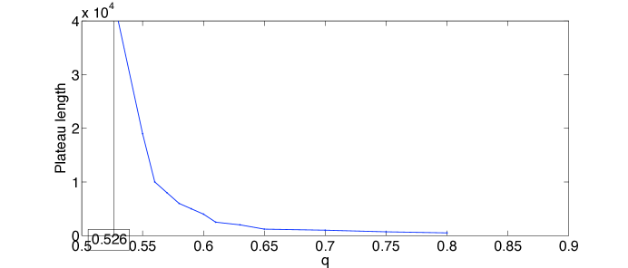
Figure 9: Plateau length $PL_{c,q}^{N}(0.005)$ for different values of q=0.8,…,0.53; Here c=0.1, N=1000. Value $0.5263$ corresponds to the theoretical bound for $q$ (given $c$).

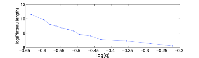
Figure 10: Log-log plot: q =0.8,…,0.5263; c=0.1, N=1000;

In Figures 9 and 10 one can see that $PL_{c,q}^{N}$ grows exponentially as $q$ decreases towards $0.5$. Recall that in the case $q\leq 0.5$, a random walk does not have ANY qsd . The exponential growth of $PL_{c,q}^{N}$ in $c$ and $q$ is a strong evidence of metastability. We conjecture that FVRW indeed has uncountably many metastable states. As $N\to\infty$ each metastable state corresponds to a qsd $\nu_{c}$.

5 Discussion

In this paper we have studied a Fleming-Viot particle system driven by a random walk on ${\mathbb{N}}$. The simulations are performed based on the Algorithm FVRW that arose from a graphical construction of the process. It would be very interesting to obtain better analytical results in any of the directions pursued here. Our findings strongly suggest that mean normalized densities of the FVRW process converge to the minimal quasi-stationary distribution of the random walk, $\nu_{0}$. This property is often referred to as selection principle.

Furthermore, we presented evidence that FVRW exhibits metastability phenomena. Moreover, it has uncountable many metastable states. In the case of infinitely many particles, any qsd of the random walk: $\nu_{c}$, $c>0$, corresponds to a metastable state of the FVRW particle system. These results give a new, physical interpretation of $\nu_{c}$, otherwise lacking in the literature. These theoretical distributions can now be seen in relation to dynamics of particle systems providing clear physical understanding and making them more applicable for problems in statistical physics.

Acknowledgements We are thankful to Gunter Schütz for inspiring discussions. Support from the National Science Foundation (grant DMS - 1007823) is gratefully acknowledged.

References

- [1] Amine Asselah, Pablo A. Ferrari, and Pablo Groisman. Quasi-stationary distributions and Fleming-Viot processes in finite spaces. arXiv: 0904.3039, 2009.
- [2] Amine Asselah, Pablo A. Ferrari, Pablo Groisman, and Matthieu Jonckheere. Fleming-Viot selects the minimal quasi-stationary distribution: The Galton-Watson case. arXiv:1206.6114, June 2012.
- [3] Amine Asselah and Marie-Noémie Thai. A note on the rightmost particle in a Fleming-Viot process. arXiv:1212.4168v1, 2012.
- [4] Krzysztof Burdzy, Robert Holyst, and Peter March. A Fleming-Viot Particle Representation of the Dirichlet Laplacian. Communications in Mathematical Physics, 214(3):679–703, November 2000.
- [5] James A. Cavender. Quasi-stationary distributions of birth-and-death processes. Advances in Applied Probability, 10(3):570–586, 1978.
- [6] PA Ferrari, H Kesten, S Martinez, P Picco, et al. Existence of quasi-stationary distributions. a renewal dynamical approach. The Annals of Probability, 23(2):501–521, 1995.
- [7] Pablo A. Ferrari and Nevena Marić. Quasi stationary distributions and Fleming-Viot processes in countable spaces . Electron. J. Probab, 12(24):684–702, 2007.
- [8] Wendell Fleming and Michel Viot. Some Measure-Valued Markov Processes in Population Genetics Theory. Indiana University Mathematics Journal, 28(5):817–843, 1979.
- [9] Pablo Groisman and Matthieu Jonckheere. Simulation of quasi-stationary distributions on countable spaces. arXiv:1206.6712, 2012.
- [10] Pablo Groisman and Matthieu Jonckheere. Front propagation and quasi-stationary distributions : the same selection principle? arXiv:1304.4847, 2013.
- [11] T. E. Harris. Additive Set-Valued Markov Processes and Graphical Methods. The Annals of Probability, 6(3):355–378, 1978.
- [12] Thomas M. Liggett. Stochastic Interacting Systems: Contact, Voter and Exclusion Processes. Springer, 1999.
- [13] Thomas M. Liggett. T. E. Harris’ contributions to interacting particle systems and percolation. The Annals of Probability, 39(2):407–416, March 2011.
- [14] Nevena Marić. Quasi-stationary distributions and Fleming-Viot processes. PhD thesis, Universidade de Sao Paulo, 2006.
- [15] A. Rákos, M. Paessens, and G. M. Schütz. Hysteresis in One-Dimensional Reaction-Diffusion Systems. Physical Review Letters, 91(23):238302, December 2003.
- [16] Denis Villemonais. Minimal quasi-stationary distribution approximation for a birth and death process. arXiv: 1404.6648, April 2014.