LTLf and LDLf Monitoring

Abstract

Runtime monitoring is one of the central tasks to provide operational decision support to running business processes, and check on-the-fly whether they comply with constraints and rules. We study runtime monitoring of properties expressed in ltl on finite traces (ltl_f) and in its extension ldl_f. ldl_f is a powerful logic that captures all monadic second order logic on finite traces, which is obtained by combining regular expressions and ltl_f, adopting the syntax of propositional dynamic logic (pdl). Interestingly, in spite of its greater expressivity, ldl_f has exactly the same computational complexity of ltl_f. We show that ldl_f is able to capture, in the logic itself, not only the constraints to be monitored, but also the de-facto standard RV-LTL monitors. This makes it possible to declaratively capture monitoring metaconstraints, and check them by relying on usual logical services instead of ad-hoc algorithms. This, in turn, enables to flexibly monitor constraints depending on the monitoring state of other constraints, e.g., “compensation” constraints that are only checked when others are detected to be violated. In addition, we devise a direct translation of ldl_f formulas into nondeterministic automata, avoiding to detour to Büchi automata or alternating automata, and we use it to implement a monitoring plug-in for the ProM suite.

1 Introduction

Runtime monitoring is one of the central tasks to provide operational decision support [20] to running business processes, and check on-the-fly whether they comply with constraints and rules. In order to provide well-founded and provably correct runtime monitoring techniques, this area is usually rooted into that of verification, the branch of formal analysis aiming at checking whether a system meets some property of interest. Being the system dynamic, properties are usually expressed by making use of modal operators accounting for the time.

Among all the temporal logics used in verification, Linear-time Temporal Logic (ltl) is particularly suited for monitoring, as an actual system execution is indeed linear. However, the ltl semantics is given in terms of infinite traces, hence monitoring must check whether the current trace is a prefix of an infinite trace, that will never be completed [2]. In several context, and in particular often in BPM, we can assume that the trace of the system is if face finite [17]. For this reason, finite-trace variant of the ltl have been introduced. Here we use the logic ltl_f (LTL on finite traces), investigated in detail in [4], and at the base of one of the main declarative process modeling approaches: declare [17, 15, 9]. Following [9], monitoring in ltl_f amounts to checking whether the current execution belongs to the set of admissible prefixes for the traces of a given ltl_f formula $\varphi$. To achieve such a task, $\varphi$ is usually first translated into a finite-state automaton for $\varphi$, which recognizes all those finite executions that satisfy $\varphi$.

Despite the presence of previous operational decision support techniques to monitoring ltl_f constraints over finite traces [9, 10], two main challenges have not yet been tackled in a systematic way. First of all, several alternative semantics have been proposed to make LTL suitable for runtime verification (such as the de-facto standard RV monitor conditions [2]), but no comprehensive technique based on finite-state automata is available to accommodate them. On the one hand, runtime verification for such logics typically considers finite partial traces whose continuation is however infinite [2], with the consequence that the corresponding techniques detour to Büchi automata for building the monitors. On the other hand, the incorporation of such semantics in the BPM setting (where also continuations are finite) has only been tackled so far with effective but ad-hoc techniques (cf. the “coloring” of automata in [9] to support the RV conditions), without a corresponding formal underpinning.

A second, key challenge is the incorporation of advanced forms of monitoring, where some constraints become of interest only in specific, critical circumstances (such as the violation of other constraints). This is the basis for supporting monitoring of compensation constraints and so-called contrary-to-duty obligations [19], i.e., obligations that are put in place only when other obligations have not been fulfilled. While this feature is considered to be a fundamental compliance monitoring functionality [8], it is still an open challenge, without any systematic approach able to support it at the level of the constraint specification language.

In this paper, we attack these two challenges by studying runtime monitoring of properties expressed in ltl_f and in its extension ldl_f [4]. ldl_f is a powerful logic that captures all monadic second order logic on finite traces, which is obtained by combining regular expressions and ltl_f, adopting the syntax of propositional dynamic logic (pdl). Interestingly, in spite of its greater expressivity, ldl_f has exactly the same computational complexity of ltl_f. We show that ldl_f is able to capture, in the logic itself, not only the usual ldl_f constraints to be monitored, but also the de-facto standard RV monitor conditions. Indeed given an ldl_f formula $\phi$, we show how to construct the ldl_f formulas that captures whether prefixes of $\phi$ satisfy the various RV monitor conditions. This, in turn, makes it possible to declaratively capture monitoring metaconstraints, and check them by relying on usual logical services instead of ad-hoc algorithms. Metaconstraints provide a well-founded, declarative basis to specify and monitor constraints depending on the monitoring state of other constraints, such as “compensation” constraints that are only checked when others are violated.

Interestingly, in doing so we devise a direct translation of ldl_f (and hence of ltl_f) formulas into nondeterministic automata, which avoid the usual detour to Büchi automata. The technique is grounded on alternating automata (afw), but it actually avoids also their introduction all together, and directly produces a standard non-deterministic finite-state automaton (nfa). Notably, such technique has been concretely implemented, and embedded into a monitoring plug-in for the ProM, which supports checking ldl_f constraints and metaconstraints.

2 ltl_f and ldl_f

In this paper we will adopt the standard ltl and its variant ldl interpreted over on finite runs.

ltl on finite traces, called ltl_f [4], has exactly the same syntax as ltl on infinite traces [18]. Namely, given a set of $\mathcal{P}$ of propositional symbols, ltl_f formulas are obtained through the following:

$$\varphi::=\phi\mid\lnot\varphi\mid\varphi_{1}\land\varphi_{2}\mid\varphi_{1}\lor\varphi_{2}\mid\raisebox{-1.1625pt}{\LARGE$\circ$}\varphi\mid\raisebox{-1.1625pt}{\LARGE$\bullet$}\varphi\mid\Diamond\varphi\mid\Box\varphi\mid\varphi_{1}\mathop{\mathcal{U}}\varphi_{2}$$

where $\phi$ is a propositional formuala over $\mathcal{P}$, $\circ$ is the next operator, $\bullet$ is weak next, $\Diamond$ is eventually, $\Box$ is always, $\mathop{\mathcal{U}}$ is until.

It is known that ltl_f is as expressive as First Order Logic over finite traces, so strictly less expressive than regular expressons which in turn are as expressive as Monadic Second Order logic over finite traces. On the other hand, regular expressions are a too low level formalism for expressing temporal specifications, since, for example, they miss a direct construct for negation and for conjunction [4].

To overcome this difficulties, in [4] Linear Dynamic Logic of Finite Traces, or ldl_f, has been proposed. This logic is as natural as ltl_f but with the full expressive power of Monadic Second Order logic over finite traces. ldl_f is obtained by merging ltl_f with regular expression through the syntax of the well-know logic of programs pdl, Propositional Dynamic Logic, [6, 7] but adopting a semantics based on finite traces. This logic is an adaptation of ldl, introduced in [21], which, like ltl, is interpreted over infinite traces.

Formally, ldl_f formulas are built as follows:

$$\begin{array}[]{lcl}\varphi&::=&\phi\mid\mathit{tt}\mid\mathit{ff}\mid\lnot\varphi\mid\varphi_{1}\land\varphi_{2}\mid\varphi_{1}\land\varphi_{2}\mid\langle\rho\rangle\varphi\mid[\rho]\varphi\\ \rho&::=&\phi\mid\varphi?\mid\rho_{1}+\rho_{2}\mid\rho_{1};\rho_{2}\mid\rho^{*}\end{array}$$

where $\phi$ is a propositional formula over $\mathcal{P}$; $\mathit{tt}$ and $\mathit{ff}$ denote respectively the true and the false ldl_f formula (not to be confused with the propositional formula $\mathit{true}$ and $\mathit{false}$), $\rho$ denotes path expressions, which are re_f expressions over propositional formulas $\phi$, with the addition of the test construct $\varphi?$ typical of pdl; and $\varphi$ stand for ldl_f formulas built by applying boolean connectives and the modal connectives $\langle\rho\rangle\varphi$ and $[\rho]\varphi$. In fact $[\rho]\varphi\equiv\lnot\langle\rho\rangle{\lnot\varphi}$.

Intuitively, $\langle\rho\rangle\varphi$ states that, from the current step in the trace, there exists an execution satisfying the regular expression $\rho$ such that its last step satisfies $\varphi$. While $[\rho]\varphi$ states that, from the current step, all executions satisfying the regular expression $\rho$ are such that their last step satisfies $\varphi$. Tests are used to insert into the execution path checks for satisfaction of additional ldl_f formulas.

As for ltl_f, the semantics of ldl_f is given in terms of finite traces denoting a finite, possibly empty, sequence of consecutive steps in the trace, i.e., finite words $\pi$ over the alphabet of $2^{\mathcal{P}}$, containing all possible propositional interpretations of the propositional symbols in $\mathcal{P}$. We denote by $\pi(i)$ the $i$th step in the trace. If the trace is shorter and does not include an $i$th step $\pi(i)$ is undefined. We denote by $\pi(i,j)$ the segment of the trace $\pi$ starting at $i$th step end ending at the $j$th step (included). If $i$ or $j$ are out of range wrt the trace that $\pi(i,j)$ is undefined, except $\pi(i,i)=\epsilon$ (i.e., the empty trace).

The semantics of ldl_f is as follows: an ldl_f formula $\varphi$ is true at a step $i$, in symbols $\pi,i\models\varphi$, as follows:

• $\pi,i\models\mathit{tt}$

• $\pi,i\not\models\mathit{ff}$

• $\pi,i\models\phi$  iff  $1\leq i\leq\mathit{n}$ and $\pi(i)\models\phi$  ($\phi$ propositional).

• $\pi,i\models\lnot\varphi$  iff  $\pi,i\not\models\varphi$.

• $\pi,i\models\varphi_{1}\land\varphi_{2}$  iff  $\pi,i\models\varphi_{1}$ and $\pi,i\models\varphi_{2}$.

• $\pi,i\models\varphi_{1}\lor\varphi_{2}$  iff  $\pi,i\models\varphi_{1}$ or $\pi,i\models\varphi_{2}$.

• $\pi,i\models\langle\rho\rangle\varphi$  iff  for some $i$ we have $\pi(i,j)\in\mathcal{L}(\rho)$ and $\pi,j\models\varphi$.

• $\pi,i\models[\rho]\varphi$  iff  for all $i$ such that $\pi(i,j)\in\mathcal{L}(\rho)$ we have $\pi,j\models\varphi$.

The relation $\pi(i,j)\in\mathcal{L}(\rho)$ is defined inductively as follows:

• $\pi(i,j)\in\mathcal{L}(\phi)$ if $j=i+1\leq\mathit{n}\;\text{and}\;\pi(i)\models\phi\quad\mbox{($\phi$ propositional)}$

• $\pi(i,j)\in\mathcal{L}(\varphi?)$ if $j=i\;\text{and}\;\pi,i\models\varphi$

• $\pi(i,j)\in\mathcal{L}(\rho_{1}+\rho_{2})$ if $\pi(i,j)\in\mathcal{L}(\rho_{1})\;\text{or}\;\pi(i,j)\in\mathcal{L}(\rho_{2})$

• $\pi(i,j)\in\mathcal{L}(\rho_{1};\rho_{2})$ if $\mbox{ exists }k\mbox{ s.t.\ }\pi(i,k)\in\mathcal{L}(\rho_{1})\mbox{ and }\pi(k,j)\in\mathcal{L}(\rho_{2})$

• $\pi(i,j)\in\mathcal{L}(\rho^{*})$ if $j=i\;\text{or}\mbox{ exists }k\mbox{ s.t.\ }\pi(i,k)\in\mathcal{L}(\rho)\mbox{ and }\pi(k,j)\in\mathcal{L}(\rho^{*})$

Observe that for $i>\mathit{n}$, hence e.g., for $\pi=\epsilon$ we get:

• $\pi,i\models\mathit{tt}$

• $\pi,i\not\models\mathit{ff}$

• $\pi,i\lnot\models\phi$  ($\phi$ propositional).

• $\pi,i\models\lnot\varphi$  iff  $\pi,i\not\models\varphi$.

• $\pi,i\models\varphi_{1}\land\varphi_{2}$  iff  $\pi,i\models\varphi_{1}$ and $\pi,i\models\varphi_{2}$.

• $\pi,i\models\varphi_{1}\lor\varphi_{2}$  iff  $\pi,i\models\varphi_{1}$ or $\pi,i\models\varphi_{2}$.

• $\pi,i\models\langle\rho\rangle\varphi$  iff  $\pi(i,i)\in\mathcal{L}(\rho)$ and $\pi,i\models\varphi$.

• $\pi,i\models[\rho]\varphi$  iff  $\pi(i,i)\in\mathcal{L}(\rho)$ implies $\pi,i\models\varphi$.

The relation $\pi(i,i)\in\mathcal{L}(\rho)$ with $i>\mathit{n}$ is defined inductively as follows:

• $\pi(i,i)\not\in\mathcal{L}(\phi)\quad\mbox{($\phi$ propositional)}$

• $\pi(i,i)\in\mathcal{L}(\varphi?)$ if $\pi,i\models\varphi$

• $\pi(i,i)\in\mathcal{L}(\rho_{1}+\rho_{2})$ if $\pi(i,i)\in\mathcal{L}(\rho_{1})\;\text{or}\;\pi(i,i)\in\mathcal{L}(\rho_{2})$

• $\pi(i,i)\in\mathcal{L}(\rho_{1};\rho_{2})$ if $\pi(i,i)\in\mathcal{L}(\rho_{1})\mbox{ and }\pi(i,i)\in\mathcal{L}(\rho_{2})$

• $\pi(i,i)\in\mathcal{L}(\rho^{*})$

Notice we have the usual boolean equivalences such as $\varphi_{1}\lor\varphi_{2}\equiv\lnot\varphi_{1}\land\lnot\varphi_{2}$, furthermore we have that: $\phi\equiv\langle\phi\rangle\mathit{tt}$, and $[\rho]\varphi\equiv\lnot\langle\rho\rangle\lnot\varphi$. It is also convenient to introduce the following abbreviations:

• $\mathit{end}=[\mathit{true}?]\mathit{ff}$ that denotes that the traces is been completed (the remaining trace is $\epsilon$ the empty one)

• $\mathit{last}=\langle\mathit{true}\rangle\mathit{end}$, which denotes the last step of the trace.

It easy to encode ltl_f into ldl_f: it suffice to observe that we can express the various ltl_f operators by recursively applying the following translations:

• $\raisebox{-1.1625pt}{\LARGE$\circ$}\varphi$ translates to $\langle\mathit{true}\rangle\varphi$;

• $\raisebox{-1.1625pt}{\LARGE$\bullet$}\varphi$ translates to $\lnot\langle\mathit{true}\rangle\lnot\varphi=[true]\varphi$ (notice that $\raisebox{-1.1625pt}{\LARGE$\bullet$}a$ is translated into $[\mathit{true}][\lnot a]\mathit{ff}$, since $a$ is equivalent to $\langle a\rangle\mathit{tt}$);

• $\Diamond\varphi$ translates to $\langle\mathit{true}^{*}\rangle\varphi$;

• $\Box\varphi$ translates to $[\mathit{true}^{*}]\varphi$ (notice that $\Box a$ is translated into $[\mathit{true}^{*}][\lnot a]\mathit{ff}$);

• $\varphi_{1}\mathop{\mathcal{U}}\varphi_{2}$ translates to $\langle(\varphi_{1}?;\mathit{true})^{*}\rangle\varphi_{2}$.

It is also easy to encode regular expressions, used as a specification formalism for traces into ldl_f: $\rho$ translates to $\langle\rho\rangle\mathit{end}$.

We say that a trace satisfies an ltl_f or ldl_f formula $\varphi$, written $\pi\models\varphi$ if $\pi,1\models\varphi$. (Note that if $\pi$ is the empty trace, and hence $1$ is out of range, still the notion of $\pi,1\models\varphi$ is well defined). Also sometimes we denote by $\mathcal{L}(\varphi)$ the set of traces that satisfy $\varphi$: $\mathcal{L}(\varphi)=\{\pi\mid\pi\models\varphi\}$.

3 ldl_f Automaton

We can associate with each ldl_f formula $\varphi$ an (exponential) nfa $A_{\varphi}$ that accepts exactly the traces that make $\varphi$ true. Here, we provide a simple direct algorithm for computing the nfa corresponding to an ldl_f formula. The correctness of the algorithm is based on the fact that (i) we can associate with each ldl_f formula $\varphi$ a polynomial alternating automaton on words (afw) $\mathcal{A}_{\varphi}$ which accepts exactly the traces that make $\varphi$ true [4], and (ii) every afw can be transformed into an nfa, see, e.g., [4]. However, to formulate the algorithm we do not need these notions, but we can work directly on the ldl_f formula. In order to proceed with the construction of the afw $\mathcal{A}_{\varphi}$, we put ldl_f formulas $\varphi$ in negation normal form $\mathit{nnf}(\varphi)$ by exploiting equivalences and pushing negation inside as much as possible, until is eliminated except in propositional formulas. Note that computing $\mathit{nnf}(\varphi)$ can be done in linear time. In other words, wlog, we consider as syntax for ldl_f the one in the previous section but without negation. Then we define an auxiliary function $\delta$ that takes an ldl_f formula $\psi$ (in negation normal form) and a propositional interpretation $\Pi$ for $\mathcal{P}$ (including $\mathit{last}$), or a special symbol $\epsilon$, returning a positive boolean formula whose atoms are (quoted) $\psi$ subformulas.

$$\delta(\texttt{"}\mathit{tt}\texttt{"},\Pi) =\mathit{true}$$

$$\delta(\texttt{"}\mathit{ff}\texttt{"},\Pi) =\mathit{false}$$

$$\delta(\texttt{"}\phi\texttt{"},\Pi) =\left\{\begin{array}[]{l}\mathit{true}\mbox{ if }\Pi\models\phi\\ \mathit{false}\mbox{ if }\Pi\not\models\phi\end{array}\right.\quad\mbox{($\phi$ propositional)}$$

$$\delta(\texttt{"}\varphi_{1}\land\varphi_{2}\texttt{"},\Pi) =\delta(\texttt{"}\varphi_{1}\texttt{"},\Pi)\land\delta(\texttt{"}\varphi_{2}\texttt{"},\Pi)$$

$$\delta(\texttt{"}\varphi_{1}\lor\varphi_{2}\texttt{"},\Pi) =\delta(\texttt{"}\varphi_{1}\texttt{"},\Pi)\lor\delta(\texttt{"}\varphi_{2}\texttt{"},\Pi)$$

$$\delta(\texttt{"}\langle\phi\rangle\varphi\texttt{"},\Pi) =\left\{\begin{array}[]{l}\texttt{"}\varphi\texttt{"}\mbox{ if }\mathit{last}\not\in\Pi\mbox{ and }\Pi\models\phi\quad\mbox{($\phi$ propositional)}\\ \delta(\texttt{"}\varphi\texttt{"},\epsilon)\mbox{ if }\mathit{last}\in\Pi\mbox{ and }\Pi\models\phi\\ \mathit{false}\mbox{ if }\Pi\not\models\phi\end{array}\right.$$

$$\delta(\texttt{"}\langle\psi?\rangle{\varphi}\texttt{"},\Pi) =\delta(\texttt{"}\psi\texttt{"},\Pi)\land\delta(\texttt{"}\varphi\texttt{"},\Pi)$$

$$\delta(\texttt{"}\langle\rho_{1}+\rho_{2}\rangle{\varphi}\texttt{"},\Pi) =\delta(\texttt{"}\langle\rho_{1}\rangle\varphi\texttt{"},\Pi)\lor\delta(\texttt{"}\langle\rho_{2}\rangle\varphi\texttt{"},\Pi)$$

$$\delta(\texttt{"}\langle\rho_{1};\rho_{2}\rangle{\varphi}\texttt{"},\Pi) =\delta(\texttt{"}\langle\rho_{1}\rangle\langle\rho_{2}\rangle\varphi\texttt{"},\Pi)$$

$$\delta(\texttt{"}\langle\rho^{*}\rangle\varphi\texttt{"},\Pi) =\left\{\begin{array}[]{l}\delta(\texttt{"}\varphi\texttt{"},\Pi)\hfill\mbox{if $\rho$ is test-only}\\ \delta(\texttt{"}\varphi\texttt{"},\Pi)\lor\delta(\texttt{"}\langle\rho\rangle\langle\rho^{*}\rangle\varphi\texttt{"},\Pi)\;\;\hfill\mbox{o/w}\end{array}\right.$$

$$\delta(\texttt{"}[\phi]\varphi\texttt{"},\Pi) =\left\{\begin{array}[]{l}\texttt{"}\varphi\texttt{"}\mbox{ if }\mathit{last}\not\in\Pi\mbox{ and }\Pi\models\phi\quad\mbox{($\phi$ propositional)}\\ \delta(\texttt{"}\varphi\texttt{"},\epsilon)\mbox{ if }\mathit{last}\in\Pi\mbox{ and }\Pi\models\phi\quad\mbox{($\phi$ propositional)}\\ \mathit{true}\mbox{ if }\Pi\not\models\phi\end{array}\right.$$

$$\delta(\texttt{"}[\psi?]{\varphi}\texttt{"},\Pi) =\delta(\texttt{"}\mathit{nnf}(\lnot\psi)\texttt{"},\Pi)\lor\delta(\texttt{"}\varphi\texttt{"},\Pi)$$

$$\delta(\texttt{"}[\rho_{1}+\rho_{2}]{\varphi}\texttt{"},\Pi) =\delta(\texttt{"}[\rho_{1}]\varphi\texttt{"},\Pi)\land\delta(\texttt{"}[\rho_{2}]\varphi\texttt{"},\Pi)$$

$$\delta(\texttt{"}[\rho_{1};\rho_{2}]{\varphi}\texttt{"},\Pi) =\delta(\texttt{"}[\rho_{1}][\rho_{2}]\varphi\texttt{"},\Pi)$$

$$\delta(\texttt{"}[\rho^{*}]\varphi\texttt{"},\Pi) =\left\{\begin{array}[]{ll}\delta(\texttt{"}\varphi\texttt{"},\Pi)\hfill\mbox{if $\rho$ is test-only}\\ \delta(\texttt{"}\varphi\texttt{"},\Pi)\land\delta(\texttt{"}[\rho][\rho^{*}]\varphi\texttt{"},\Pi)\;\;\hfill\mbox{o/w}\end{array}\right.$$

where $\delta(\texttt{"}\varphi\texttt{"},\epsilon)$, i.e., the interpretation of ldl_f formula in the case the (remaining fragment of the) trace is empty, is defined as follows:

$$\delta(\texttt{"}\mathit{tt}\texttt{"},\epsilon) =\mathit{true}$$

$$\delta(\texttt{"}\mathit{ff}\texttt{"},\epsilon) =\mathit{false}$$

$$\delta(\texttt{"}\phi\texttt{"},\epsilon) =\mathit{false}\quad\mbox{($\phi$ propositional)}$$

$$\delta(\texttt{"}\varphi_{1}\land\varphi_{2}\texttt{"},\epsilon) =\delta(\texttt{"}\varphi_{1}\texttt{"},\epsilon)\land\delta(\texttt{"}\varphi_{2}\texttt{"},\epsilon)$$

$$\delta(\texttt{"}\varphi_{1}\lor\varphi_{2}\texttt{"},\epsilon) =\delta(\texttt{"}\varphi_{1}\texttt{"},\epsilon)\lor\delta(\texttt{"}\varphi_{2}\texttt{"},\epsilon)$$

$$\delta(\texttt{"}\langle\phi\rangle\varphi\texttt{"},\epsilon) =\mathit{false}\quad\mbox{($\phi$ propositional)}$$

$$\delta(\texttt{"}\langle\psi?\rangle{\varphi}\texttt{"},\epsilon) =\delta(\texttt{"}\psi\texttt{"},\epsilon)\land\delta(\texttt{"}\varphi\texttt{"},\epsilon)$$

$$\delta(\texttt{"}\langle\rho_{1}+\rho_{2}\rangle{\varphi}\texttt{"},\epsilon) =\delta(\texttt{"}\langle\rho_{1}\rangle\varphi\texttt{"},\epsilon)\lor\delta(\texttt{"}\langle\rho_{2}\rangle\varphi\texttt{"},\epsilon)$$

$$\delta(\texttt{"}\langle\rho_{1};\rho_{2}\rangle{\varphi}\texttt{"},\epsilon) =\delta(\texttt{"}\langle\rho_{1}\rangle\langle\rho_{2}\rangle\varphi\texttt{"},\epsilon)$$

$$\delta(\texttt{"}\langle\rho^{*}\rangle\varphi\texttt{"},\epsilon) =\delta(\texttt{"}\varphi\texttt{"},\epsilon)$$

$$\delta(\texttt{"}[\phi]\varphi\texttt{"},\epsilon) =\mathit{true}\quad\mbox{($\phi$ propositional)}$$

$$\delta(\texttt{"}[\psi?]{\varphi}\texttt{"},\epsilon) =\delta(\texttt{"}\mathit{nnf}(\lnot\psi)\texttt{"},\epsilon)\lor\delta(\texttt{"}\varphi\texttt{"},\epsilon)$$

$$\delta(\texttt{"}[\rho_{1}+\rho_{2}]{\varphi}\texttt{"},\epsilon) =\delta(\texttt{"}[\rho_{1}]\varphi\texttt{"},\epsilon)\land\delta(\texttt{"}[\rho_{2}]\varphi\texttt{"},\epsilon)$$

$$\delta(\texttt{"}[\rho_{1};\rho_{2}]{\varphi}\texttt{"},\epsilon) =\delta(\texttt{"}[\rho_{1}][\rho_{2}]\varphi\texttt{"},\epsilon)$$

$$\delta(\texttt{"}[\rho^{*}]\varphi\texttt{"},\epsilon) =\delta(\texttt{"}\varphi\texttt{"},\epsilon)$$

Notice also that for $\phi$ propositional, $\delta(\texttt{"}\phi\texttt{"},\Pi)=\delta(\texttt{"}\langle\phi\rangle\mathit{tt}\texttt{"},\Pi)$ and $\delta(\texttt{"}\phi\texttt{"},\epsilon)=\delta(\texttt{"}\langle\phi\rangle\mathit{tt}\texttt{"},\epsilon)$, as a consequence of the equivalence $\phi\equiv\langle\phi\rangle\mathit{tt}$.

1:algorithm ldl_f2nfa()

2:input ltl_f formula $\varphi$

3:output nfa $A_{\varphi}=(2^{\mathcal{P}},\mathcal{S},\{s_{0}\},\varrho,\{s_{f}\})$

4:$s_{0}\leftarrow\{\texttt{"}\varphi\texttt{"}\}$ $\triangleright$ single initial state

5:$s_{f}\leftarrow\emptyset$ $\triangleright$ single final state

6:$\mathcal{S}\leftarrow\{s_{0},s_{f}\}$, $\varrho\leftarrow\emptyset$

7:while ($\mathcal{S}$ or $\varrho$ change) do

8:   if ($q\in\mathcal{S}$ and $q^{\prime}\models\bigwedge_{(\texttt{"}\psi\texttt{"}\in q)}\delta(\texttt{"}\psi\texttt{"},\Theta)$) then

9:      $\mathcal{S}\leftarrow\mathcal{S}\cup\{q^{\prime}\}$ $\triangleright$ update set of states

10:      $\varrho\leftarrow\varrho\cup\{(q,\Theta,q^{\prime})\}$ $\triangleright$ update transition relation    

Figure 1: nfa construction

Using the auxiliary function $\delta$ we can build the nfa $A_{\varphi}$ of an ldl_f formula $\varphi$ in a forward fashion as described in Figure 1), where: states of $A_{\varphi}$ are sets of atoms (recall that each atom is quoted $\varphi$ subformulas) to be interpreted as a conjunction; the empty conjunction $\emptyset$ stands for $\mathit{true}$; $\Theta$ is either a propositional interpretation $\Pi$ over $\mathcal{P}$ or the empty trace $\epsilon$ (this gives rise to epsilon transition either to true or false) and $q^{\prime}$ is a set of quoted subformulas of $\varphi$ that denotes a minimal interpretation such that $q^{\prime}\models\bigwedge_{(\texttt{"}\psi\texttt{"}\in q)}\delta(\texttt{"}\psi\texttt{"},\Theta)$. (Note: we do not need to get all $q$ such that $q^{\prime}\models\bigwedge_{(\texttt{"}\psi\texttt{"}\in q)}\delta(\texttt{"}\psi\texttt{"},\Theta)$, but only the minimal ones.) Notice that trivially we have $(\emptyset,a,\emptyset)\in\varrho$ for every $a\in\Sigma$.

The algorithm ldl_f2nfa terminates in at most exponential number of steps, and generates a set of states $\mathcal{S}$ whose size is at most exponential in the size of $\varphi$.

Theorem 3.1

Let $\varphi$ be an ldl_f formula and $A_{\varphi}$ the nfa constructed as above. Then $\pi\models\varphi\mbox{ iff }\pi\in L(A_{\varphi})$ for every finite trace $\pi$.

Proof (sketch).  Given a ldl_f formula $\varphi$, $\delta$ grounded on the subformulas of $\varphi$ becomes the transition function of the afw, with initial state $\texttt{"}\varphi\texttt{"}$ and no final states, corresponding to $\varphi$ [4]. Then ldl_f2nfa essentially transforms the afw into a nfa. ∎

Notice that above we have assumed to have a special proposition $\mathit{last}\in\mathcal{P}$. If we want to remove such an assumption, we can easily transform the obtained automaton $A_{\varphi}=(2^{\mathcal{P}},\mathcal{S},\{\texttt{"}\varphi\texttt{"}\},\varrho,\{\emptyset\})$ into the new automaton

$$A^{\prime}_{\varphi}=(2^{\mathcal{P}-\{\mathit{last}\}},\mathcal{S}\cup\{\textit{ended}\},\{\texttt{"}\varphi\texttt{"}\},\varrho^{\prime},\{\emptyset,\textit{ended}\})$$

where: $(q,\Pi^{\prime},q^{\prime})\in\varrho^{\prime}$ iff $(q,\Pi^{\prime},q^{\prime})\in\varrho$, or $(q,\Pi^{\prime}\cup\{\mathit{last}\},\mathit{true})\in\varrho$ and $q^{\prime}=\textit{ended}$.

It is easy to see that the nfa obtained can be built on-the-fly while checking for nonemptiness, hence we have:

Theorem 3.2

Satisfiability of an ldl_f formula can be checked in PSPACE by nonemptiness of $A_{\varphi}$ (or $A^{\prime}_{\varphi}$).

Considering that it is known that satisfiability in ldl_f is a PSPACE-complete problem we can conclude that the proposed construction is optimal wrt computational complexity for satisfiability, as well as for validity and logical implication which are linearly reducible to satisfiability in ldl_f (see [4] for details).

4 Run-time Monitoring

From an high-level perspective, the monitoring problem amounts to observe an evolving system execution and report the violation or satisfaction of properties of interest at the earliest possible time. As the system progresses, its execution trace increases, and at each step the monitor checks whether the trace seen so far conforms to the properties, by considering that the execution can still continue. This evolving aspect has a significant impact on the monitoring output: at each step, indeed, the outcome may have a degree of uncertainty due to the fact that future executions are yet unknown.

Several variant of monitoring semantics have been proposed (see [2] for a survey). In this paper we adopt the semantics in [9], which is basically the finite-trace variant of the RV semantics in [2]: Given a ltl_f or ldl_f formula $\varphi$, each time the system evolves, the monitor returns one among the following truth values:

• $[\varphi]_{RV}=\mathit{temp\_true}$, meaning that the current execution trace temporarily satisfies $\varphi$, i.e., it is currently compliant with $\varphi$, but there is a possible system future prosecution which may lead to falsify $\varphi$;

• $[\varphi]_{RV}=\mathit{temp\_false}$, meaning that the current trace temporarily falsify $\varphi$, i.e., $\varphi$ is not current compliant with $\varphi$, but there is a possible system future prosecution which may lead to satisfy $\varphi$;

• $[\varphi]_{RV}=\mathit{true}$, meaning that the current trace satisfies $\varphi$ and it will always do, no matter how it proceeds;

• $[\varphi]_{RV}=\mathit{false}$, meaning that the current trace falsifies $\varphi$ and it will always do, no matter how it proceeds.

The first two conditions are unstable because they may change into any other value as the system progresses. This reflects the general unpredictability of system possible executions. Conversely, the other two truth values are stable since, once outputted, they will not change anymore. Observe that a stable truth value can be reached in two different situations: (i) when the system execution terminates; (ii) when the formula that is being monitored can be fully evaluated by observing a partial trace only. The first case is indeed trivial, as when the execution ends, there are no possible future evolutions and hence it is enough to evaluate the finite (and now complete) trace seen so far according to the ldl_f semantics. In the second case, instead, it is irrelevant whether the systems continues its execution or not, since some ldl_f properties, such as eventualities or safety properties, can be fully evaluated as soon as something happens, e.g., when the eventuality is verified or the safety requirement is violated. Notice also that when a stable value is outputted, the monitoring analysis can be stopped.

From a more theoretical viewpoint, given an ldl_f property $\varphi$, the monitor looks at the trace seen so far, assesses if it is a prefix of a complete trace not yet completed, and categorizes it according to its potential for satisfying or violating $\varphi$ in the future. We call a prefix possibly good for an ldl_f formula $\varphi$ if there exists an extension of it which satisfies $\varphi$. More precisely, given an ldl_f formula $\varphi$, we define the set of possibly good prefixes for $\mathcal{L}(\varphi)$ as the set

$$\mathcal{L}_{\mathit{poss\_good}}(\varphi)=\{\pi\mid\exists\pi^{\prime}.\pi\pi^{\prime}\in\mathcal{L}(\varphi)\}$$ (1)

Prefixes for which every possible extension satisfies $\varphi$ are instead called necessarily good. More precisely, given an ldl_f formula $\varphi$, we define the set of necessarily good prefixes for $\mathcal{L}(\varphi)$ as the set

$$\mathcal{L}_{\mathit{nec\_good}}(\varphi)=\{\pi\mid\forall\pi^{\prime}.\pi\pi^{\prime}\in\mathcal{L}(\varphi)\}.$$ (2)

The set of necessarily bad prefixes $\mathcal{L}_{\mathit{nec\_bad}}(\varphi)$ can be defined analogously as

$$\mathcal{L}_{\mathit{nec\_bad}}(\varphi)=\{\pi\mid\forall\pi^{\prime}.\pi\pi^{\prime}\not\in\mathcal{L}(\varphi)\}.$$ (3)

Observe that the necessarily bad prefixes for $\varphi$ are the necessarily good prefixes for $\neg\varphi$, i.e., $\mathcal{L}_{\mathit{nec\_bad}}(\varphi)=\mathcal{L}_{\mathit{nec\_good}}(\lnot\varphi)$.

Using this language theoretic notions, we can provide a precise characterization of the semantics four standard monitoring evaluation functions [9].

Proposition 1

Let $\varphi$ be an ldl_f formula and $\pi$ a trace. Then:

• $\pi\models[\varphi]_{RV}=\mathit{temp\_true}$ iff $\pi\in\mathcal{L}(\varphi)\setminus\mathcal{L}_{\mathit{nec\_good}}(\varphi)$;

• $\pi\models[\varphi]_{RV}=\mathit{temp\_false}$ iff $\pi\in\mathcal{L}(\neg\varphi)\setminus\mathcal{L}_{\mathit{nec\_bad}}(\varphi)$;

• $\pi\models[\varphi]_{RV}=\mathit{true}$ iff $\pi\in\mathcal{L}_{\mathit{nec\_good}}(\varphi)$;

• $\pi\models[\varphi]_{RV}=\mathit{false}$ iff $\pi\in\mathcal{L}_{\mathit{nec\_bad}}(\varphi)$.

Proof (sketch).  Immediate from the definitions in [9] and the language theoretic definitions above. ∎

We close this section by exploiting the language theoretic notions to better understand the relationships between the various kinds of prefixes. We start by observing that, the set of all finite words over the alphabet $2^{\mathcal{P}}$ is the union of the language of $\varphi$ and its complement $\mathcal{L}(\varphi)\cup\mathcal{L}(\neg\varphi)=(2^{\mathcal{P}})^{*}$. Also, any language and its complement are disjoint $\mathcal{L}(\varphi)\cap\mathcal{L}(\neg\varphi)=\emptyset$.

Since from the definition of possibly good prefixes we have $\mathcal{L}(\varphi)\subseteq\mathcal{L}_{\mathit{poss\_good}}(\varphi)$ and $\mathcal{L}(\neg\varphi)\subseteq\mathcal{L}_{\mathit{poss\_good}}(\neg\varphi)$, we also have that $\mathcal{L}_{\mathit{poss\_good}}(\varphi)\cup\mathcal{L}_{\mathit{poss\_good}}(\neg\varphi)=(2^{\mathcal{P}})^{*}$. Also from the definition it is easy to see that $\mathcal{L}_{\mathit{poss\_good}}(\varphi)\cap\mathcal{L}_{\mathit{poss\_good}}(\neg\varphi)=\{\pi\mid\exists\pi^{\prime}.\pi\pi^{\prime}\in\mathcal{L}(\varphi)\land\exists\pi^{\prime\prime}.\pi\pi^{\prime\prime}\in\mathcal{L}(\neg\varphi)\}$ meaning that the set of possibly good prefixes for $\varphi$ and the set of possibly good prefixes for $\neg\varphi$ do intersect, and in such an intersection are paths that can be extended to satisfy $\varphi$ but can also be extended to satisfy $\neg\varphi$. It is also easy to see that $\mathcal{L}(\varphi)=\mathcal{L}_{\mathit{poss\_good}}(\varphi)\setminus\mathcal{L}(\neg\varphi).$

Turning to necessarily good prefixes and necessarily bad prefixes, it is easy to see that $\mathcal{L}_{\mathit{nec\_good}}(\varphi)=\mathcal{L}_{\mathit{poss\_good}}(\varphi)\setminus\mathcal{L}_{\mathit{poss\_good}}(\neg\varphi)$, that $\mathcal{L}_{\mathit{nec\_bad}}(\varphi)=\mathcal{L}_{\mathit{poss\_good}}(\neg\varphi)\setminus\mathcal{L}_{\mathit{poss\_good}}(\varphi)$, and also that $\subseteq\mathcal{L}(\varphi)\;\;\text{and}\;\;\mathcal{L}_{\mathit{nec\_good}}(\varphi)\not\subseteq\mathcal{L}(\neg\varphi)$.

Interestingly, necessarily good, necessarily bad, possibly good prefixes partition all finite traces. Namely

Proposition 2

The set of all traces $(2^{\mathcal{P}})^{*}$ can be partitioned into

$$\begin{array}[]{l@{\qquad\quad}c@{\qquad\quad}r}\mathcal{L}_{\mathit{nec\_good}}(\varphi)&\mathcal{L}_{\mathit{poss\_good}}(\varphi)\cap\mathcal{L}_{\mathit{poss\_good}}(\neg\varphi)&\mathcal{L}_{\mathit{nec\_bad}}(\varphi)\end{array}$$

$$\text{such that }\begin{array}[t]{l}\mathcal{L}_{\mathit{nec\_good}}(\varphi)\cup(\mathcal{L}_{\mathit{poss\_good}}(\varphi)\cap\mathcal{L}_{\mathit{poss\_good}}(\neg\varphi))\cup\mathcal{L}_{\mathit{nec\_bad}}(\varphi)=(2^{\mathcal{P}})^{*}\\ \mathcal{L}_{\mathit{nec\_good}}(\varphi)\cap(\mathcal{L}_{\mathit{poss\_good}}(\varphi)\cap\mathcal{L}_{\mathit{poss\_good}}(\neg\varphi))\cap\mathcal{L}_{\mathit{nec\_bad}}(\varphi)=\emptyset.\end{array}$$

Proof (sketch).  Follows from the definitions of the necessarily good, necessarily bad, possibly good prefixes of $\mathcal{L}(\varphi)$ and $\mathcal{L}(\lnot\varphi)$. ∎

5 Runtime Monitors in ldl_f

As discussed in the previous section the core issue in monitoring is prefix recognition. ltl_f is not expressive enough to talk about prefixes of its own formulas. Roughly speaking, given a ltl_f formula, the language of its possibly good prefixes for cannot be in general described as an ltl_f formula. For such a reason, building a monitor usually requires direct manipulation of the automaton for $\phi$.

ldl_f instead can capture any nondeterministic automata as a formula, and it has the capability of expressing properties on prefixes. We can exploit such an extra expressivity to capture the monitoring condition in a direct and elegant way. We start by showing how to construct formulas representing (the language of) prefixes of other formulas, and then we prove how use them for the monitoring problem.

More precisely, given an ldl_f formula $\varphi$, it is possible to express the language $\mathcal{L}_{possgood}(\varphi)$ with an ldl_f formula $\varphi^{\prime}$. Such a formula is obtained in two steps.

Lemma 1

Given a ldl_f formula $\varphi$, there exists a regular expression $\mathsf{pref}_{\varphi}$ such that $\mathcal{L}(\mathsf{pref}_{\varphi})=\mathcal{L}_{\mathit{poss\_good}}(\varphi)$.

Proof (sketch).  The proof is constructive. We can build the nfa $\mathcal{A}$ for $\varphi$ following the procedure in [4]. We then set as final all states of $\mathcal{A}$ from which there exists a non-zero length path to a final state. This new finite state machine $\mathcal{A}_{\mathit{poss\_good}}(\varphi)$ is such that $\mathcal{L}(\mathcal{A}_{\mathit{poss\_good}}(\varphi))=\mathcal{L}_{\mathit{poss\_good}}(\varphi)$. Since nfa are exactly as expressive as regular expressions, we can translate $\mathcal{A}_{\mathit{poss\_good}}(\varphi)$ to a regular expression $\mathsf{pref}_{\varphi}$. ∎

Given that ldl_f is as expressive as regular expression (cf. [4]), we can translate $\mathsf{pref}_{\varphi}$ into an equivalent ldl_f formula, as the following states.

Theorem 5.1

Given a ldl_f formula $\varphi$,

$$\begin{array}[]{l}\pi\in\mathcal{L}_{\mathit{poss\_good}}(\varphi)\;\text{iff}\;\pi\models\langle\mathsf{pref}_{\varphi}\rangle\mathit{end}\\ \pi\in\mathcal{L}_{\mathit{nec\_good}}(\varphi)\;\text{iff}\;\pi\models\langle\mathsf{pref}_{\varphi}\rangle\mathit{end}\land\lnot\langle\mathsf{pref}_{\lnot\varphi}\rangle\mathit{end}\\ \end{array}$$

Proof (sketch).  Any regular expression $\rho$, and hence any regular language, can be captured in ldl_f as $\langle\rho\rangle\mathit{end}$. Hence the language $\mathcal{L}_{\mathit{nec\_good}}(\varphi)$ can be captured by $\langle\mathsf{pref}_{\varphi}\rangle\mathit{end}$ and the language $\mathcal{L}_{\mathit{nec\_good}}(\varphi)$ which is equivalent $\mathcal{L}_{\mathit{poss\_good}}(\varphi)\setminus\mathcal{L}_{\mathit{poss\_good}}(\neg\varphi)$ can be captured by captured by $\langle\mathsf{pref}_{\varphi}\rangle\mathit{end}\land\lnot\langle\mathsf{pref}_{\lnot\varphi}\rangle\mathit{end}$. ∎

In other words, given a ldl_f formula $\varphi$, formula $\varphi^{\prime}=\langle\mathsf{pref}_{\varphi}\rangle\mathit{end}$ is a ldl_f formula such that $\mathcal{L}(\varphi^{\prime})=\mathcal{L}_{possgood}(\varphi)$. Similarly for $\mathcal{L}_{\mathit{nec\_good}}(\varphi)$.

Exploiting this result, and the results in Proposition 1, we reduce RV monitoring to the standard evaluation of ldl_f formulas over a (partial) trace. Formally:

Theorem 5.2

Let $\pi$ be a (typically partial) trace. The following equivalences hold:

• $\pi\models[\varphi]_{RV}=\mathit{temp\_true}$  iff  $\pi\models\varphi\land\langle\mathsf{pref}_{\lnot\varphi}\rangle\mathit{end}$;

• $\pi\models[\varphi]_{RV}=\mathit{temp\_false}$  iff  $\pi\models\lnot\varphi\land\langle\mathsf{pref}_{\varphi}\rangle\mathit{end}$;

• $\pi\models[\varphi]_{RV}=\mathit{true}$  iff  $\langle\mathsf{pref}_{\varphi}\rangle\mathit{end}\land\lnot\langle\mathsf{pref}_{\lnot\varphi}\rangle\mathit{end}$;

• $\pi\models[\varphi]_{RV}=\mathit{false}$  iff  $\langle\mathsf{pref}_{\lnot\varphi}\rangle\mathit{end}\land\lnot\langle\mathsf{pref}_{\varphi}\rangle\mathit{end}$.

Proof (sketch).  Follows from Proposition 1 and Theorem 5.1 using the language theoretic equivalences discussed in Secton 4. ∎

6 Monitoring Declare Constraints and Metaconstraints

We now ground our monitoring approach to the case of declare monitoring. declare is a language and framework for the declarative, constraint-based modelling of processes and services. A thorough treatment of constraint-based processes can be found in [16, 12]. As a modelling language, declare takes a complementary approach to that of classical, imperative process modeling, in which all allowed control-flows among tasks must be explicitly represented, and every other execution trace is implicitly considered as forbidden. Instead of this procedural and “closed” approach, declare has a declarative, “open” flavor: the agents responsible for the process execution can freely choose how to perform the involved tasks, provided that the resulting execution trace complies with the modeled business constraints. This is the reason why, alongside traditional control-flow constraints such as sequence (called in declare chain succession), declare supports a plethora of peculiar constraints that do not impose specific temporal orderings, or that explicitly account with negative information, i.e., prohibition of task execution.

Given a set $\mathcal{P}$ of tasks, a declare model is a set $\mathcal{C}$ of ltl_f (and hence ldl_f) constraints over $\mathcal{P}$, used to restrict the allowed execution traces. Among all possible ltl_f constraints, some specific patterns have been singled out as particularly meaningful for expressing declare processes, taking inspiration from [5]. Such patterns are grouped into four families: (i) existence(unary) constraints, stating that the target task must/cannot be executed (a certain amount of times); (ii) choice(binary) constraints, modeling choice of execution; (iii) relation(binary) constraints, modeling that whenever the source task is executed, then the target task must also be executed (possibly with additional requirements); (iv) negation(binary) constraints, modeling that whenever the source task is executed, then the target task is prohibited (possibly with additional restrictions). Table 1 reports some of these patterns.

Example 1

Consider a fragment of a purchase order process, where we consider three key business constraints. First, an order can be closed at most once. In declare, this can be tackled with a absence 2 constraint, visually and formally represented as:

$$\overset{0..1}{\framebox{~{}{{close order}}~{}}}\qquad\varphi_{close}=\neg\Diamond(\textnormal{{close order}}\land\raisebox{-1.1625pt}{\LARGE$\circ$}\Diamond\textnormal{{close order}})$$

Second, an order can be canceled only until it is closed. This can be captured by a negation succession constraint, which states that after the order is closed, it cannot be canceled anymore:

$$\mbox{\framebox{~{}{{close order}}~{}}{\mbox{$\bullet\relbar\relbar\blacktriangleright\bullet$}}$\lVert$\hskip 9.79996pt\framebox{~{}{{cancel order}}~{}}}\qquad\varphi_{canc}=\Box(\textnormal{{close order}}\mathbin{\rightarrow}\neg\Diamond\textnormal{{cancel order}})$$

Finally, after the order is closed, it becomes possible to do supplementary payments, for various reasons (e.g., to speed up the delivery of the order).

$$\mbox{\framebox{~{}{{close order}}~{}}{\mbox{$\relbar\relbar\relbar\blacktriangleright\bullet$}}\framebox{~{}{{pay suppl}}~{}}}~{}\varphi_{pay}=(\neg\textnormal{{pay suppl}}\mathop{\mathcal{U}}\textnormal{{close order}})\lor\neg\Diamond\textnormal{{close order}}$$

Beside modeling and enactment of constraint-based processes, previous works have also focused on runtime verification of declare models. A family of declare monitoring approaches rely on the original ltl_f formalization of declare, and employ corresponding automata-based techniques to track running process instances and check whether they satisfy the modeled constraints or not [9, 10]. Such techniques have been in particular used for:

• Monitoring single declare constraints so as to provide a fine-grained feedback; this is done by adopting the RV semantics for ltl_f, and tracking the evolution each constraint through the four RV truth values.

• Monitoring the global declare model by considering all its constraints together (i.e., constructing a dfa for the conjunction of all constraints); this is important for computing the early detection of violations, i.e., violations that cannot be explicitly found in the execution trace collected so far, but that cannot be avoided in the future.

We now discuss how ldl_f can be adopted for monitoring declare constraints, with a twofold advantage. First, as shown in Section 5, ldl_f is able to encode the RV semantics directly into the logic, without the need of introducing ad-hoc modifications in the corresponding standard logical services. Second, beside being able to reconstruct all the aforementioned monitoring techniques, our approach also provides a declarative, well-founded basis for monitoring metaconstraints, i.e., constraints that involve both the execution of tasks and the monitoring outcome obtained by checking other constraints.

Monitoring Declare Constraints with ldl_f.

Since ldl_f includes ltl_f, declare constraints can be directly encoded in ldl_f using their standard formalization [17, 15]. Thanks to the translation into nfas discussed in Section 3 (and, if needed, their determinization into corresponding dfas), the obtained automaton can then be used to check whether a (partial) finite trace satisfies this constraint or not. This is not very effective, as the approach does not support the detection of fine-grained truth values as those of RV. By relying on Theorem 5.2, however, we can reuse the same technique, this time supporting all RV. In fact, by formalizing the good prefixes of each declare pattern, we can immediately construct the four ldl_f formulas that embed the different RV truth values, and check the current trace over each of the corresponding automata. Table 1 reports the good prefix characterization of some of the declare patterns; it can be seamlessly extended to all other patterns as well.

Example 2

Let us consider the absence 2 constraint $\varphi_{close}$ in Example 1. Following Table 1, its good prefix characterization is $\mathsf{pref}_{\varphi_{close}}=o^{*}+(o^{*};\textnormal{{close order}};o^{*})$, where $o$ is a shortcut for all the tasks involved in the purchase order process but close order. This can be used to construct the four formulas mentioned in Theorem 5.2, which in turn provide the basis to produce, e.g., the following result:

	start	do “close order”	do “pay suppl.”	do “close order”
$\overset{0..1}{\framebox{~{}{{close order}}~{}}}$	$\mathit{temp\_true}$			$\mathit{false}$

Observe that this baseline approach can be extended along a number of directions. For example, as shown in Table 1, the majority of declare patterns does not cover all the four RV truth values. This is the case, e.g., for absence 2, which can never be evaluated to be $\mathit{true}$ (since it is always possible to continue the execution so as to perform a twice), nor to $\mathit{temp\_false}$ (the only way of violating the constraint is to perform a twice, and in this case it is not possible to “repair” to the violation anymore). This information can be used to restrict the generation of the automata only to those cases that are relevant to the constraint. Furthermore, it is possible to reconstruct exactly the approach in [9], where every state in the dfas corresponding to the constraints to be monitored, is enriched with a “color” accounting for one of the four RV truth values. To do so, we have simply to combine the four dfas generated for each constraint. This is possible because such dfas are generated from formulas built on top of the good prefix characterization of the original formula, and hence they all produce the same automaton, but with different final states. In fact, this observation provides a formal justification to the correctness of the approach in [9].

Table 1: Some declare constraints, together with their prefix characterization, minimal bad prefix charaterization, and possible RV states; for each constraint, $o$ is a shortcut for “other tasks”, i.e., tasks not involved in the constraint itself.

	name	notation	$\mathsf{pref}$	possible RV states
existence​​​​	Existence	$\overset{1..\ast}{\framebox{~{}{{a}}~{}}}$	$(a+o)^{*}$	$\mathit{temp\_false}$, $\mathit{true}$
	Absence 2	$\overset{0..1}{\framebox{~{}{{a}}~{}}}$	$o^{*}+(o^{*};a;o^{*})$	$\mathit{temp\_true}$, $\mathit{false}$
choice	Choice	a $\relbar$$\relbar$ $\lozenge$ $\relbar$$\relbar$ b	$(a+b+o)^{*}$	$\mathit{temp\_false}$, $\mathit{true}$
	Exclusive Choice	a $\relbar$$\relbar$ $\blacklozenge$ $\relbar$$\relbar$ b	$(a+o)^{*}+(b+o)^{*}$	$\mathit{temp\_false}$, $\mathit{temp\_true}$, $\mathit{false}$
relation	Resp. existence	a $\bullet\relbar\relbar\relbar\relbar$ b	$(a+b+o)^{*}$	$\mathit{temp\_true}$, $\mathit{temp\_false}$, $\mathit{true}$
	Coexistence	a $\bullet\relbar\relbar\relbar\bullet$ b	$(a+b+o)^{*}$	$\mathit{temp\_true}$, $\mathit{temp\_false}$, $\mathit{true}$
	Response	a $\bullet\relbar\relbar\relbar\blacktriangleright$ b	$(a+b+o)^{*}$	$\mathit{temp\_true}$, $\mathit{temp\_false}$
	Precedence	a $\relbar\relbar\relbar\blacktriangleright\bullet$ b	$o^{*};(a;(a+b+o)^{*})^{*}$	$\mathit{temp\_true}$, $\mathit{true}$, $\mathit{false}$
	Succession	a $\bullet\relbar\relbar\blacktriangleright\bullet$ b	$o^{*};(a;(a+b+o)^{*})^{*}$	$\mathit{temp\_true}$, $\mathit{temp\_false}$, $\mathit{false}$
negation	Not Coexistence	a $\bullet\relbar\relbar\relbar\bullet$$\lVert$    b	$(a+o)^{*}+(b+o)^{*}$	$\mathit{temp\_true}$, $\mathit{false}$
	Neg. Succession	a $\bullet\relbar\relbar\blacktriangleright\bullet$$\lVert$    b	$(b+o)^{*};(a+o)^{*}$	$\mathit{temp\_true}$, $\mathit{false}$

Metaconstraints.

Thanks to the ability of ldl_f to directly encode into the logic declare constraints but also their RV monitoring states, we can formalize metaconstraints that relate the RV truth values of different constraints. Intuitively, such metaconstraints allow one to capture that we become interested in monitoring some constraint only when other constraints are evaluated to be in a certain RV truth value. This, in turn, provides the basis to declaratively capture two classes of properties that are of central importance in the context of runtime verification:

• Compensation constraints, that is, constraints that should be enforced by the agents executing the process in the case other constraints are violated, i.e., are evaluated to be $\mathit{false}$. Previous works have been tackled this issue through ad-hoc techniques, with no declarative counterpart [9, 10].

• Recovery mechanisms resembling contrary-to-duty obligations in legal reasoning [19], i.e., obligations that are put in place only when other obligations are not met.

Technically, a generic form for metaconstraints is the pattern $\Phi_{pre}\mathbin{\rightarrow}\Psi_{exp}$, where:

• $\Phi_{pre}$ is a boolean formula, whose atoms are membership assertions of the involved constraints to the RV truth values;

• $\Psi_{exp}$ is a boolean formula whose atoms are the constraints to be enforced when $\Phi_{pre}$ evaluates to true.

This pattern can be used, for example, to state that whenever constraints $c_{1}$ and $c_{2}$ are permanently violated, then either constraint $c_{3}$ or $c_{4}$ have to be enforced. Observe that the metaconstraint so constructed is a standard ldl_f formula. Hence, we can reapply Theorem 5.2 to it, getting four ldl_f formulas that can be used to track the evolution of the metaconstraint among the four RV values.

Example 3

Consider the declare constraints of Example 1. We want to enhance it with a compensation constraint stating that whenever $\varphi_{canc}$ is violated (i.e., the order is canceled after it has been closed), then a supplement payment must be issued. This can be easily captured in ldl_f as follows. First of all, we model the compensation constraint, which corresponds, in this case, to a standard existence constraint over the pay supplement task. Let $\varphi_{dopay}$ denote the ltl_f formalization of such a compensation constraint. Second, we capture the intended compensation behavior by using the following ldl_f metaconstraint:

$$\{[\varphi_{canc}]_{RV}=\mathit{false}\}\mathbin{\rightarrow}\varphi_{dopay}$$

which, leveraging Theorem 5.2, corresponds to the standard ldl_f formula:

$$\footnotesize(\langle\mathsf{pref}_{\lnot\varphi_{canc}}\rangle\mathit{end}\land\lnot\langle\mathsf{pref}_{\varphi_{canc}}\rangle\mathit{end})\mathbin{\rightarrow}\varphi_{dopay}$$

A limitation of this form of metaconstraint is that the right-hand part $\Psi_{exp}$ is monitored from the beginning of the trace. This is acceptable in many cases. E.g., in Example 3, it is ok if the user already paid a supplement before the order cancelation caused constraint $\varphi_{canc}$ to be violated. In other situations, however, this is not satisfactory, because we would like to enforce the compensating behavior only after $\Phi_{pre}$ evaluates to true, e.g., after the violation of a given constraint has been detected. In general, we can extend the aforementioned metaconstraint pattern as follows: $\Phi_{pre}\mathbin{\rightarrow}[\rho]\Psi_{exp}$, where $\rho$ is a regular expression denoting the paths after which $\Psi_{exp}$ is expected to be enforced.

By constructing $\rho$ as the regular expression accounting for the paths that make $\Phi_{pre}$ true, we can then exploit this improved metaconstraint to express that $\Psi_{exp}$ is expected to become true after all prefixes of the current trace that made $\Phi_{pre}$ true.

Example 4

We modify the compensation constraint of Example 3, so as to reflect that when a closed order is canceled (i.e., $\varphi_{canc}$ is violated), then a supplement must be paid afterwards. This is captured by the following metaconstraint:

$$\{[\varphi_{canc}]_{RV}=\mathit{false}\}\mathbin{\rightarrow}[\mathit{re}_{\{[\varphi_{canc}]_{RV}=\mathit{false}\}}]\varphi_{dopay}$$

where $\mathit{re}_{\{[\varphi_{canc}]=\mathit{false}\}}$ denotes the regular expression for the language $\mathcal{L}(\{[\varphi_{canc}]=\mathit{false}\})=\mathcal{L}(\langle\mathsf{pref}_{\lnot\varphi_{canc}}\rangle\mathit{end}\land\lnot\langle\mathsf{pref}_{\varphi_{canc}}\rangle\mathit{end})$. This regular expression describes all paths containing a violation for constraint $\varphi_{canc}$.

7 Implementation

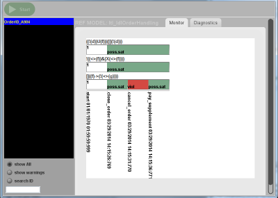
Figure 2: Screenshot of our operational support provider’s output.

The entire approach has been implemented as an operational decision support (OS) provider for the ProM 6 process mining framework. ProM 6 provides a generic OS environment [22] that supports the interaction between an external workflow management systems at runtime (producing events) and ProM. In particular, it provides an OS service that receives a stream of events from the external world, updates and orchestrates the registered OS providers implementing different types of online analysis to be applied on the stream, and reports the produced results back to the external world.

At the back-end of the plug-in, there is a software module specifically dedicated to the construction and manipulation of nfas from ldl_f formulas, concretely implementing the technique presented in Section 3. To manipulate regular expressions and automata, we used the fast, well-known library dk.brics.automaton [11].

Figure 2 shows a graphical representation of the evolution of constraints described in Example 1 of Section 6 when monitored using our operational support provider. In the ldl_f formulas, the literals $f$, $g$ and $d$ respectively stand for tasks close order, cancel order, and pay supplement.

8 Conclusion

We can see the approach proposed in this paper, as an extension of the declarative process specification approach, at the basis of declare, to (i) more powerful specification logics (ldl_f, i.e., Monadic Second Order logics over finite traces , instead of ltl_f, i.e., First Order logic logics over finite traces), (ii) to monitoring constraints. Notably, this declarative approach to monitoring supports seamlessly monitoring metaconstraints, i.e., constraints that do not only predicate about the dynamics of task executions, but also about the truth values of other constraints. We have grounded this approach on declare itself, showing how to declaratively specify compensation constraints.

The next step will be to incorporate recovery mechanisms into the approach, in particular providing a formal underpinning to the ad-hoc recovery mechanisms studied in [9]. Furthermore, we intend to extend our approach to data-aware business constraints [1, 13], mixing temporal operators with first-order queries over the data attached to the monitored events. This setting has been studied using the Event Calculus [13, 14], also considering some specific forms of compensation in declare [3]. However, the resulting approach can only query the partial trace accumulated so far, and not reason upon its possible future continuations, as automata-based techniques are able to do. To extend the approach presented here to the case of data-aware business constraints, we will build on recent, interesting decidability results for the static verification of data-aware business processes against sophisticated variants of first-order temporal logics [1].

Acknowledgments.

This research has been partially supported by the EU IP project Optique: Scalable End-user Access to Big Data, grant agreement n. FP7-318338, and by the Sapienza Award 2013 “spiritlets: Spiritlet-based smart spaces”.

References

- [1] B. Bagheri Hariri, D. Calvanese, G. De Giacomo, A. Deutsch, and M. Montali. Verification of relational data-centric dynamic systems with external services. In Proc. of the 32nd ACM SIGACT SIGMOD SIGART Symp. on Principles of Database Systems (PODS), 2013.
- [2] A. Bauer, M. Leucker, and C. Schallhart. Comparing LTL Semantics for Runtime Verification. Logic and Computation, 2010.
- [3] F. Chesani, P. Mello, M. Montali, and P. Torroni. Verification of choreographies during execution using the reactive event calculus. In 5th Int. Workshop on Web Services and Formal Methods (WS-FM), volume 5387 of LNCS. Springer, 2008.
- [4] G. De Giacomo and M. Y. Vardi. Linear temporal logic and linear dynamic logic on finite traces. In Proc. of the 23rd Int. Joint Conf. on Artificial Intelligence (IJCAI). AAAI, 2013.
- [5] M. B. Dwyer, G. S. Avrunin, and J. C. Corbett. Patterns in property specifications for finite-state verification. In B. W. Boehm, D. Garlan, and J. Kramer, editors, Proc. of the 1999 International Conf. on Software Engineering (ICSE). ACM Press, 1999.
- [6] M. J. Fischer and R. E. Ladner. Propositional dynamic logic of regular programs. Journal of Computer and System Science, 18, 1979.
- [7] D. Harel, D. Kozen, and J. Tiuryn. Dynamic Logic. MIT Press, 2000.
- [8] L. T. Ly, F. M. Maggi, M. Montali, S. Rinderle-Ma, and W. M. P. van der Aalst. A framework for the systematic comparison and evaluation of compliance monitoring approaches. In Proc. of the 17th IEEE Int. Enterprise Distributed Object Computing Conf. (EDOC). IEEE, 2013.
- [9] F. M. Maggi, M. Montali, M. Westergaard, and W. M. P. van der Aalst. Monitoring business constraints with linear temporal logic: An approach based on colored automata. In Proc. of the 9th Int. Conf. on Business Process Management (BPM), volume 6896 of LNCS. Springer, 2011.
- [10] F. M. Maggi, M. Westergaard, M. Montali, and W. M. P. van der Aalst. Runtime verification of ltl-based declarative process models. In Proc. of the 2nd Int. Conf. on Runtime Verification (RV), volume 7186 of LNCS. Springer, 2012.
- [11] A. Møller. dk.brics.automaton – finite-state automata and regular expressions for Java, 2010. http://www.brics.dk/automaton/.
- [12] M. Montali. Specification and Verification of Declarative Open Interaction Models: a Logic-Based Approach, volume 56 of LNBIP. Springer, 2010.
- [13] M. Montali, F. Chesani, F. M. Maggi, and P. Mello. Towards data-aware constraints in declare. In S. Y. Shin and J. C. Maldonado, editors, Proc. of the 28th Symposium On Applied Computing (SAC). ACM Press, 2013.
- [14] M. Montali, F. M. Maggi, F. Chesani, P. Mello, and W. M. P. van der Aalst. Monitoring business constraints with the event calculus. ACM Trans. on Intelligent Systems and Technology, 5(1), 2013.
- [15] M. Montali, M. Pesic, W. M. P. van der Aalst, F. Chesani, P. Mello, and S. Storari. Declarative specification and verification of service choreographies. ACM Trans. on the Web, 4(1), 2010.
- [16] M. Pesic. Constraint-Based Workflow Management Systems: Shifting Controls to Users. PhD thesis, Beta Research School for Operations Management and Logistics, Eindhoven, 2008.
- [17] M. Pesic and W. M. P. van der Aalst. A declarative approach for flexible business processes management. In Proc. of the BPM 2006 Workshops, volume 4103 of LNCS. Springer, 2006.
- [18] A. Pnueli. The temporal logic of programs. In Proc. of the 18th Ann. Symp. on Foundations of Computer Science (FOCS). IEEE, 1977.
- [19] H. Prakken and M. J. Sergot. Contrary-to-duty obligations. Studia Logica, 57(1), 1996.
- [20] W. M. P. van der Aalst. Process Mining - Discovery, Conformance and Enhancement of Business Processes. Springer, 2011.
- [21] M. Vardi. The rise and fall of linear time logic, 2011. 2nd Int’l Symp. on Games, Automata, Logics and Formal Verification.
- [22] M. Westergaard and F. Maggi. Modelling and Verification of a Protocol for Operational Support using Coloured Petri Nets. In Proc. of ATPN, 2011.