Proposed method for laser spectroscopy of pionic helium atoms to determine the charged-pion mass

Abstract

Metastable pionic helium ($\pi{\rm He}^{+}$) is a three-body atom composed of a helium nucleus, an electron occupying the $1s$ ground state, and a negatively charged pion $\pi^{-}$ in a Rydberg state with principal- and orbital angular momentum quantum numbers of $n\sim\ell+1\sim 16$. We calculate the spin-independent energies of the $\pi{\rm{}^{3}He}^{+}$ and $\pi{\rm{}^{4}He}^{+}$ isotopes in the region $n=15$-19. These include relativistic and quantum electrodynamics corrections of orders $R_{\infty}\alpha^{2}$ and $R_{\infty}\alpha^{3}$ in atomic units, where $R_{\infty}$ and $\alpha$ denote the Rydberg and fine structure constants. The fine-structure splitting due to the coupling between the electron spin and the orbital angular momentum of the $\pi^{-}$, and the radiative and Auger decay rates of the states are also calculated. Some states $(n,\ell)=(16,15)$ and $(17,16)$ retain nanosecond-scale lifetimes against $\pi^{-}$ absorption into the helium nucleus. We propose to use laser pulses to induce $\pi^{-}$ transitions from these metastable states, to states with large ($\sim 10^{11}$ s^-1) Auger rates. The $\pi{\rm He}^{2+}$ ion that remains after Auger emission of the $1s$ electron undergoes Stark mixing with the $s$, $p$, and $d$ states during collisions with the helium atoms in the experimental target. This leads to immediate nuclear absorption of the $\pi^{-}$. The resonance condition between the laser beam and the atom is thus revealed as a sharp spike in the rates of neutrons, protons, deuterons, and tritons that emerge. A resonance curve is obtained from which the $\pi{\rm He}^{+}$ transition frequency can in principle be determined with a fractional precision of $10^{-8}-10^{-6}$ provided that the systematic uncertainties can be controlled. By comparing the measured $\pi{\rm He}^{+}$ frequencies with the calculated values, the $\pi^{-}$ mass may be determined with a similar precision. The $\pi{\rm He}^{+}$ will be synthesized by allowing a high-intensity ($>10^{8}$ s^-1) beam of $\pi^{-}$　produced by a cyclotron to come to rest in a helium target. The precise time structure of the $\pi^{-}$ beam is used to ensure a sufficient rate of coincidence between the resonant laser pulses and the $\pi{\rm He}^{+}$ atoms.

I Introduction

In this paper we describe a possible method for laser spectroscopy of metastable pionic helium ($\pi{\rm He}^{+}\equiv\pi^{-}+{\rm He}^{2+}+e^{-}$). This is a hypothetical three-body atom Condo (1964); Russell (1969, 1970a); *russell1970_2; *russell1970_3 composed of a helium nucleus, an electron occupying the 1s ground state, and a negatively charged pion $\pi^{-}$ in a Rydberg state with principal and orbital angular momentum quantum numbers of around $n\sim\ell+1\sim 16$. These states are theoretically expected to retain nanosecond-scale lifetimes against the competing processes of $\pi^{-}$ absorption into the helium nucleus and $\pi^{-}\rightarrow\mu^{-}+\overline{\nu}_{\mu}$ decay to a negatively charged muon and a muon-based antineutrino. This is because the Rydberg $\pi^{-}$ orbitals have very little overlap with the nucleus, whereas the electromagnetic cascade processes that normally cause the rapid deexcitation of the $\pi^{-}$, such as radiative decay, or Auger emission of the $1s$ electron, are relatively slow. The atom should therefore be amenable to laser spectroscopic measurements of the $\pi^{-}$ transition frequencies. This would conclusively show the existence of $\pi{\rm He}^{+}$. By comparing the experimental frequencies with the results of the three-body quantum electrodynamics (QED) calculations presented in this paper, the $\pi^{-}$ mass can in principle be determined with a high precision, as in the case of antiprotonic helium atoms Hori et al. (2011); Korobov (2008).

The existence of $\pi{\rm He}^{+}$ has been indirectly inferred from four experiments Fetkovich and Pewitt (1963); Block et al. (1963, 1965); Zaĭmidoroga et al. (1967); Nakamura et al. (1992) that observed that a small fraction of $\pi^{-}$ retains an anomalously long lifetime in helium targets. Quantitative comparisons of the data with theoretical calculations have been difficult. Some sets of calculated decay rates of $\pi{\rm He}^{+}$ states differ from each other by 1–2 orders of magnitude. Nothing is experimentally known about the distribution of states which may be formed. Whereas x-ray transitions between short-lived states of low principal quantum number $n_{i}$ in the two-body pionic helium ($\pi{\rm He}^{2+}\equiv\pi^{-}+{\rm He}^{2+}$) ion have been studied for many years by fluorescence spectroscopy with an experimental precision of $\sim 10^{-4}$ Wetmore et al. (1967); Backenstoss et al. (1974); Gotta (2004), no atomic lines of the three-body $\pi{\rm He}^{+}$ have been detected so far. Many assumptions are therefore needed to design any laser spectroscopy experiment.

We propose the irradiation of the $\pi{\rm He}^{+}$ with resonant laser pulses that induce transitions from the metastable states to states with picosecond-scale lifetimes against Auger emission of the $1s$ electron. The Rydberg $\pi{\rm He}^{2+}$ ion that remains after Auger decay undergoes Stark mixing during collisions Day et al. (1960); Borie and Leon (1980); Landua and Klempt (1982) with the helium atoms in the experimental target. The electric fields induced by the collisions mix the ionic states with the $s$, $p$, and $d$ states at high $n_{i}$, that have large overlap with the helium nucleus. This leads to nuclear absorption of the $\pi^{-}$ within picoseconds. Neutrons, protons, deuterons, and tritons with kinetic energies of up to 30–90 MeV consequently emerge. By measuring these particle rates as a function of the laser frequency, the resonance condition between the laser and the $\pi{\rm He}^{+}$ is revealed in the form of a resonance curve. From this the $\pi{\rm He}^{+}$ transition frequency $\nu_{\rm exp}$ can be determined. The $\pi{\rm He}^{+}$ are synthesized by allowing a $\pi^{-}$ beam produced by the Paul Scherrer Institute (PSI) ring cyclotron Wagner et al. (2009); Adam et al. (2013) to come to rest in a helium target. The precise time structure of this beam allows the formation of $\pi{\rm He}^{+}$ in the target to be synchronized to the arrival of the resonant laser pulses. Laser beams generated by solid-state lasers with high repetition rates $f_{\rm las}=0.1$–1 kHz and average powers 1–100 W will excite the $\pi{\rm He}^{+}$.

The experiment is difficult for many reasons; in fact, laser excitation of a meson has never been observed. The metastability of $\pi^{-}$ in helium corresponds to a lifetime $\tau_{c}\sim 7$ ns Nakamura et al. (1992) which is shorter than that of any exotic atom studied by laser spectroscopy so far Karshenboim (2005), whereas the probability for inducing a $\pi^{-}$ transition is small. Some transitions involve ultraviolet wavelengths, which are not easily accessible by high-power lasers. The high-intensity $\pi^{-}$ beam ($>10^{8}$ s^-1) is characterized by large momenta ($\geq 80$ MeV/c), momentum spread (5–10$\%$), and emittances. The contaminant electrons and $\mu^{-}$ in the beam, as well as the $\pi^{-}$ that immediately undergo nuclear absorption in the experimental apparatus, may give rise to backgrounds which prevent the detection of the $\pi{\rm He}^{+}$ laser resonance signal. The passage of charged particles in the helium target causes a broad spectra of scintillation photons emitted by helium excimers McKinsey et al. (2003). This paper mainly outlines the method by which the spectroscopic signal may be resolved rather than the details of an apparatus which rejects these backgrounds.

This paper is organized in the following way. Section II reviews some past research on $\pi{\rm He}^{+}$. In Sect. III we carry out three-body QED calculations on the energy levels and fine structure of the $\pi{\rm{}^{4}He}^{+}$ and $\pi{\rm{}^{3}He}^{+}$ isotopes. Section IV discusses the formation and electromagnetic cascade of $\pi{\rm He}^{+}$. We calculate the radiative and Auger rates and simulate the population evolutions of the metastable states. Section V describes the method to detect the laser resonance. The resonance profiles of some candidate transitions are simulated. The energy distributions of the neutrons, protons, deuterons, and tritons that emerge following the nuclear absorption of $\pi^{-}$ are described in some detail. Section VI presents Monte Carlo simulations to roughly estimate the signal-to-background ratio of the laser resonance. Conclusions and a discussion concerning the determination of the $\pi^{-}$ mass are given in Sect. VII.

II Brief history

In two experiments carried out in the 1960s Fetkovich and Pewitt (1963); Block et al. (1963, 1965), $\pi^{-}$ were allowed to come to rest in liquid-helium bubble chambers. The readout photographs were scanned for any $\pi^{-}\rightarrow\mu^{-}+\overline{\nu}_{\mu}$ decay arising from $\pi^{-}$ at rest. Such events were expected to occur very rarely since the $\pi^{-}$ stopped in other target materials are normally absorbed into the atomic nuclei within picoseconds; this leaves no time for $\pi^{-}\rightarrow\mu^{-}+\overline{\nu}_{\mu}$ decay to occur with a lifetime of $\tau_{\pi}\sim 26$ ns. In the surprising case of helium targets, however, an anomalously large fraction ($\sim 10^{-2}$) of the $\pi^{-}$ were found to decay in this way. This implied that the $\pi^{-}$ were trapped into atomic orbitals that retain long lifetimes against nuclear absorption Fetkovich and Pewitt (1963); Block et al. (1963, 1965). The average cascade time from atomic formation to absorption was estimated to be $\tau_{c}=200$–400 ps, based on the measured ratio between $\pi^{-}\rightarrow\mu^{-}+\overline{\nu}_{\mu}$ decay and nuclear absorption events, which were compared with a simple model describing the formation and deexcitation of the atom. A third experiment that involved $\pi^{-}$ stopped in a diffusion chamber filled with ${}^{3}{\rm He}$ gas of pressure $p\sim 1.8\times 10^{6}$ Pa deduced a similar cascade time of $\tau_{c}=140\pm 70$ ps Zaĭmidoroga et al. (1967). Anomalous longevities were also detected for other negatively-charged particles $K^{-}$ Block et al. (1965); Fetkovich et al. (1970) and $\Sigma^{-}$ Comber et al. (1974); Fetkovich et al. (1975) stopped in liquid helium.

Condo Condo (1964) attempted to explain these results by suggesting that some of the $\pi^{-}$ forms the three-body $\pi{\rm He}^{+}$ atom via the reaction

$$\pi^{-}+{\rm He}\rightarrow\pi{\rm He}^{+}+e^{-}.$$ (1)

The principal quantum number of the initially populated states was assumed to be distributed around the value

$$n\sim n_{0}=\sqrt{\frac{M^{\ast}}{m_{e}}}.$$ (2)

Here $m_{e}$ and $M^{\ast}$ denote the electron mass and the reduced mass of the $\pi^{-}$–${\rm He}^{2+}$ pair, respectively. The $n_{0}\sim 16$ value for $\pi{\rm{}^{4}He}^{+}$ and $\pi{\rm{}^{3}He}^{+}$ corresponds to the $\pi^{-}$ orbitals with the same radius and binding energy as that of the displaced $1s$ electron in the reaction of Eq. 1. These Rydberg states are long-lived Day et al. (1960); Borie and Leon (1980); Landua and Klempt (1982); Jensen and Markushin (2002); Cohen (2004); Raeisi G. and Kalantari (2009); Popov and Pomerantsev (2012) since (i): the wave functions of the $\pi^{-}$ orbitals have very little overlap with the nucleus and so the $\pi^{-}$ cannot be directly absorbed, (ii): the states have long ($>10$ ns) lifetimes against radiative deexcitation of the $\pi^{-}$, (iii): the deexcitation to a $\pi{\rm He}^{2+}$ ionic state of principal and angular momentum quantum numbers of $n_{i}\sim 13$ and $\ell_{i}=n_{i}-1$ by Auger emission of the remaining electron

$$\pi\mathrm{He}^{+}_{(n,\ell)}\to\pi\mathrm{He}^{2+}_{(n_{i},\ell_{i})}+e^{-}$$ (3)

is suppressed because of the large binding energy ($\sim 25$ eV) of the electron and the high multipolarity $\Delta\ell_{A}=\ell-\ell_{i}\geq 3$ of the Auger transition, and (iv): with this electron in place, the $\pi^{-}$ is protected against Stark mixing during atomic collisions.

Russell Russell (1969, 1970a, 1970b, 1970c) calculated the Auger and radiative decay rates of the $\pi{\rm He}^{+}$ states. The Auger rates $A_{(15,14)}=2\times 10^{12}$ s^-1 and $A_{(16,15)}=4\times 10^{9}$ s^-1 of the states $(n,\ell)=(15,14)$ and $(16,15)$ appeared to be too large Russell (1969) to account for the observed longevity of $\pi^{-}$ in helium. Fetkovich Fetkovich et al. (1971) suggested that some $\pi^{-}$ are capture into the $n>17$ states, which have smaller Auger rates. On the other hand, they noted inconsistencies Fetkovich et al. (1971) between the experiments which deduced average cascade times of 200–400 ps in liquid-helium targets Fetkovich and Pewitt (1963); Block et al. (1963), and theoretical models of pionic atoms, which include collisional deexcitation processes that predicted a value of $\sim 20$ ps.

In 1989, an experiment at KEK directly measured the lifetime of $K^{-}$ stopped in liquid helium using particle counters Yamazaki et al. (1989). It showed that $\sim 98\%$ of the $K^{-}$ are promptly absorbed by the helium nucleus, whereas the remaining $(1.9\pm 0.3)\%$ retain a lifetime of $9.5\pm 0.3$ ns against the nuclear absorption and free decays of $K^{-}$. A similar experiment carried out at TRIUMF Nakamura et al. (1992) showed that $(2.30\pm 0.07)\%$ of the $\pi^{-}$ stopped in liquid helium retain a lifetime of $7.3\pm 0.1$ ns. These lifetimes are much longer than the average cascade times deduced by the above cloud chamber experiments. We are unaware of another measurement on the metastability of $\pi^{-}$ in helium Fetkovich and Pewitt (1963); Block et al. (1963); Zaĭmidoroga et al. (1967); Nakamura et al. (1992). Some calculations on the nonrelativistic energies and decay rates of $\pi{\rm He}^{+}$ have been presented in Ref. Obreshkov et al. (2003). The present paper will provide higher-precision values that include relativistic and QED corrections over a larger range of states.

Experimental and theoretical efforts in the last 20 years have concentrated on the antiprotonic helium ($\overline{p}{\rm He}^{+}\equiv\overline{p}+{\rm He}^{2+}+e^{-}$) atom, which retain mean lifetimes of 3–4 $\mu{\rm s}$ against antiproton annihilation in the helium nucleus Iwasaki et al. (1991). The transition frequencies of $\overline{p}{\rm He^{+}}$ were recently measured to a fractional precision of $(2.3-5)\times 10^{-9}$ Hori et al. (2011) in laser spectroscopy experiments Morita et al. (1994); Hori et al. (2001, 2003, 2006). By comparing the results with three-body QED calculations Korobov (2008), the antiproton-to-electron mass ratio was determined as $M_{\overline{p}}/m_{e}=1836.1526736(23)$ Hori et al. (2011). Most of the calculated radiative and Auger rates Korobov and Shimamura (1997); Korobov (2008) agreed with the state lifetimes measured by laser spectroscopy Hori et al. (1998a); *mhori1998e; Hori et al. (2001); Yamaguchi et al. (2002, 2004) within a precision of 10–30$\%$. A similar experiment should be possible for $\pi{\rm He}^{+}$.

III Energy level structure

III.1 Spin-independent part

As the $\pi{\rm He}^{+}$ states are unstable against Auger decay, they are properly described as pseudo- or resonant states which lie in the continuum of the non-relativistic three-body Hamiltonian, rather than truly bound states. The resonances constitute poles of the scattering matrix in the complex momentum plane, which in turn can be mapped to the unphysical sheets of the energy Riemann surface Burke (2011). Direct numerical calculation of these eigenvalues is difficult since the stationary wavefunctions exponentially diverge when the distances between the constituent particles tend to infinity. To transform the wavefunctions into convergent bound-state forms that allows the $\pi{\rm He}^{+}$ energy levels to be readily calculated, we employ the complex-coordinate rotation (CCR) method Ho (1983); Moiseyev (1998). The coordinates of the dynamical system are continued (“rotated”) to the complex plane, using the transformation $r_{ij}\rightarrow r_{ij}e^{i\varphi}$, where $\varphi$ denotes a rotational angle. Under this transformation, the Hamiltonian changes as a function of $\varphi$,

$$\hat{H}_{\varphi}=\hat{T}e^{-2i\varphi}+\hat{V}e^{-i\varphi},$$ (4)

where $\hat{T}$ and $\hat{V}$ denote the kinetic energy and Coulomb potential operators Ho (1983); Kino et al. (1998); Korobov (2003). By this analytical transformation, the continuum spectrum of the original Hamiltonian is rotated around branch points (or thresholds). The resonant poles corresponding to $\pi{\rm He}^{+}$ states are thus uncovered by branch cuts, so that they belong to the discrete spectrum of the rotated $\hat{H}_{\varphi}$. The resonance energy can be determined by solving the complex eigenvalue problem for the rotated Hamiltonian,

$$(\hat{H}_{\varphi}-E)\Psi_{\varphi}=0,$$ (5)

as the eigenfunction $\Psi_{\varphi}$ is square-integrable. The complex eigenvalue $E=E_{r}-i\Gamma/2$ defines the energy $E_{r}$ and the width $\Gamma$ of the resonance; the latter is related to the Auger rate of the state by $A=\Gamma/\hbar$, where the reduced Planck constant is denoted by $\hbar$.

As we mentioned above, the $\pi{\rm He}^{+}$ states are conventionally characterized by the approximate quantum numbers $(n,\ell)$ of the atomic $\pi^{-}$ orbital Condo (1964); Russell (1969, 1970a); *russell1970_2; *russell1970_3. The states also share the features of a polar molecule Shimamura (1992) with two nuclei ${\rm He}^{2+}$ and $\pi^{-}$, which are described by an alternative pair of quantum numbers $(v,L)$. Here $v$ denotes the vibrational quantum number, or equivalently, the number of radial nodes of the $\pi^{-}$ wavefunction. The total orbital angular momentum quantum number is denoted by $L$. As the electron occupies roughly the $1s$ state, the conversion between the two sets of quantum numbers follows,

$$v = n-\ell-1,$$ (6)

$$L = \ell.$$ (7)

The $(v,L)$ numbers are used in our representation of the variational wavefunctions. All numerical results on the state energies, lifetimes, and populations are presented using the conventional $(n,\ell)$ quantum numbers.

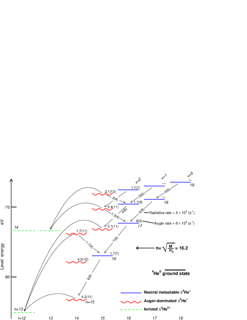
Figure 1: (Online color) Energy level diagram of $\pi{\rm{}^{4}He}^{+}$ atom. On the left-hand scale the theoretical absolute energy of each state $(n,\ell)$ is plotted relative to the three-body-breakup threshold. The wavy lines indicate Auger-dominated states with picosecond-scale lifetimes, solid lines the metastable levels with lifetimes of $>10$ ns. The Auger decay rate of each state is shown in s^-1. The dashed lines indicate the final $\pi{\rm He}^{2+}$ ionic states formed after Auger electron emission, the curved arrows some Auger transitions with minimum $|\Delta\ell_{A}|$. Radiative transitions of the types $(n,\ell)\rightarrow(n-1,\ell-1)$ and $(n,\ell)\rightarrow(n-1,\ell+1)$ are indicated using straight arrows, with the corresponding decay rates shown in s^-1.

We utilize a variational wavefunction Korobov et al. (1999) which reflects both the atomic and molecular nature of $\pi{\rm He}^{+}$. The coordinate system is shown in Fig. 1 of Ref. Korobov et al. (1999). The angular part of the wavefunction is described by the (molecular) bipolar harmonic expansion of the form

$$\Psi^{L\Lambda}_{M}(\mathbf{R},\mathbf{r})=\sum_{l+l_{e}=L}R^{l}r^{l_{e}}\{Y_{l}\otimes Y_{l_{e}}\}_{LM}G^{L\Lambda}_{ll_{e}}(R,r,\theta).$$ (8)

The components $G^{L\Lambda}_{ll_{e}}(R,r,\theta)$ are functions of the internal degrees of freedom, which can be expanded in the (atomic) exponential form

$$G^{L\Lambda}_{ll_{e}}(R,r,\theta)=\sum_{i=1}^{\infty}C_{i}e^{-\alpha_{i}R-\beta_{i}r-\gamma_{i}|\mathbf{R}-\mathbf{r}|}.$$ (9)

Here $M$ denotes the projection of the total orbital angular momentum on the $z$ axis of the fixed frame, and $\Lambda=(-1)^{L}$ the total spatial parity. The complex parameters $\alpha_{i},\beta_{i}$ and $\gamma_{i}$ are generated in a quasirandom way.

We used variational basis sets which includes 2000 functions. Tables 1 and 2 present the nonrelativistic energies and widths of the $\pi{\rm{}^{4}He}^{+}$ and $\pi{\rm{}^{3}He}^{+}$ states, respectively. The expectation values of the operators needed to evaluate the leading-order relativistic correction for the bound electron and the one-loop self-energy and vacuum polarization corrections of order $R_{\infty}\alpha^{3}$ in atomic units (see Appendix) are also shown. Here $R_{\infty}$ and $\alpha$ denote the Rydberg and fine structure constants, respectively. The numerical precision of the nonrelativistic energies (indicated in parenthesis) are better than $\sim 10^{-8}$, but the actual precision is limited to $>10^{-6}$ by the experimental uncertainty on the $\pi^{-}$ mass Beringer et al. (2012) used in these calculations,

$$M_{\pi^{-}}=139.57018(35){\rm MeV}/c^{2}.$$ (10)

The uncertainties on the Auger widths are of similar magnitude to the nonrelativistic energies since these CCR calculations evaluate the “complex energy” of Eq. 5.

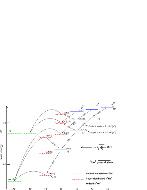
Figure 2: (Online color) Energy level diagrams of $\pi{\rm{}^{3}He}^{+}$ atom and $\pi{\rm{}^{3}He}^{2+}$ ion. See caption of Fig. 1 for details.

The energy-level diagrams of $\pi{\rm{}^{4}He}^{+}$ and $\pi{\rm{}^{3}He}^{+}$ in the $n=15$–19 regions are shown in Figs. 1 and 2. The level energies relative to the three-body breakup threshold are indicated in solid or wavy lines. Radiative transitions of the type $(n,\ell)\rightarrow(n-1,\ell-1)$ involve energy intervals of $\Delta E=2-6$ eV, whereas the energies of states with the same $n$-value increase in steps of $\Delta E=0.5-0.7$ eV for every change $\Delta\ell=+1$. This removal of the $\ell$-degeneracy suppresses Stark mixing during atomic collisions.

The energy levels of the two-body $\pi{\rm{}^{4}He}^{2+}$ and $\pi{\rm{}^{3}He}^{2+}$ ions in the regions $n_{i}=13$–14 are shown by dashed lines, superimposed on the same figures. The spin-independent parts of the $\pi{\rm He}^{2+}$ level energies can be calculated to a fractional precision better than $10^{-5}$ using the simple Bohr formula in atomic units,

$$E_{n_{i}}=-\frac{2M^{\ast}}{n_{i}^{2}},$$ (11)

where $M^{\ast}$ denotes the reduced mass of the $\pi^{-}$–${\rm He^{2+}}$ pair. Radiative transitions of the type $(n_{i},\ell_{i})\rightarrow(n_{i}-1,\ell_{i}\pm 1)$ lie in the ultraviolet ($>10$ eV) region. The $\pi^{-}$ states with the same $n_{i}$-value are now degenerate, so that Stark mixing with $s$, $p$, and $d$ states occurs during collisions with helium atoms Day et al. (1960); Borie and Leon (1980); Landua and Klempt (1982). This normally leads to $\pi^{-}$ absorption within picoseconds, although lifetimes of $\sim 100$ ns have been observed for $\overline{p}{\rm He}^{2+}$ ions formed in low-density targets where the collision rate is sufficiently low Hori et al. (2005). The short lifetime and large transition energies make it difficult to induce laser resonances in $\pi{\rm He}^{2+}$ and so we will not consider the feasibility here.

III.2 Fine structure

The boson-boson $\pi^{-}$–${\rm{}^{4}He}^{2+}$ pair has no spin-spin or spin-orbit interactions. The coupling $\mathbf{s}_{e}\cdot\mathbf{L}$ between the spin vector $\mathbf{s}_{e}$ of the 1s electron and the orbital angular momentum vector $\mathbf{L}$ of the $\pi^{-}$ splits each $\pi{\rm{}^{4}He}^{+}$ state $(n,\ell)$ into a pair of fine structure substates, which are characterized by the total angular momentum vector

$$\mathbf{J}=\mathbf{L}+\mathbf{s}_{e}.$$ (12)

This fine structure splitting is determined by the effective Hamiltonian using the corresponding operators

$$\hat{H}_{\rm eff}=E_{1}\cdot\left(\mathbf{\hat{s}}_{e}\cdot\mathbf{\hat{L}}\right),$$ (13)

where the energies $E_{1}$ (shown in Tables 1 and 2) are calculated by integrating over the spatial internal degrees of freedom. The expectation value of the scalar product in Eq. 13 may be expanded using the total angular momentum quantum number $J$ as

$$\langle\mathbf{\hat{s}}_{e}\cdot\mathbf{\hat{L}}\rangle = \frac{1}{2}\left[\langle\mathbf{\hat{J}}^{2}\rangle-\langle\mathbf{\hat{L}}^{2}\rangle-\langle\mathbf{\hat{s}}_{e}^{2}\rangle\right]$$ (14)

$$= \frac{1}{2}\left[J(J+1)-L(L+1)-3/4\right].$$

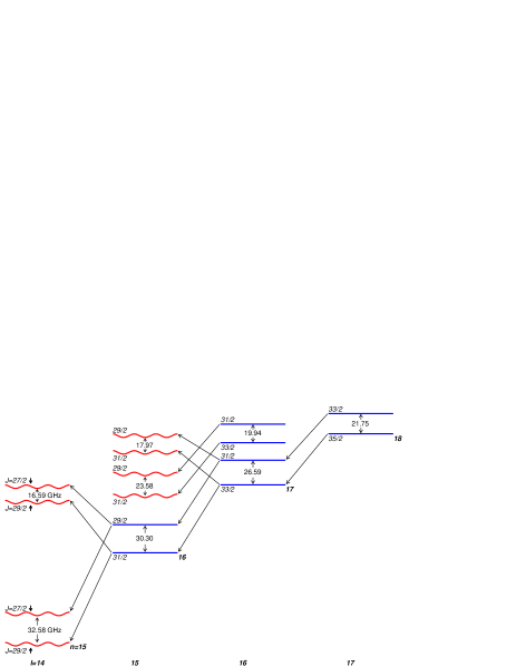
Figure 3: (Online color) Fine structure of $\pi{\rm{}^{4}He}^{+}$, indicating the principal-, orbital angular momentum-, and total angular momentum quantum numbers $n$, $\ell$, and $J$ of each substate. Wavy lines show Auger-dominated short-lived states with picosecond-scale lifetimes, solid lines metastable states with $>10$ ns lifetimes. Small bold arrows indicate the direction of the electron spin. Fine structure splittings $\Delta\nu_{\rm fs}$ of each substate pairs shown in gigahertz. Some $E1$ laser transitions that do not flip the electron spin are indicated by diagonal arrows. Drawing not to scale.

In the $n=16$–18 region (Fig. 3), the fine structure splitting increases from $\Delta\nu_{\rm fs}=16.6$ to 32.6 GHz for $\pi{\rm{}^{4}He}^{+}$ states with smaller $n$- and larger $\ell$-values. Each resonance profile for a transition of the type $(n,\ell)\rightarrow(n-1,\ell-1)$ or $(n,\ell)\rightarrow(n+1,\ell-1)$ contains a dominant pair of fine structure sublines separated by 2–5 GHz or 4–9 GHz, respectively. These sublines correspond to the pairs of $\Delta J=-1$ transitions (indicated by arrows in Fig. 3) that do not flip the electron spin. They cannot be resolved as distinct peaks for transitions that involve states with large Auger widths ($A_{(n,\ell)}/2\pi\geq 25$ GHz, wavy lines). The laser resonance profile also contains a weaker (by $\sim 10^{-2}$) subline, which corresponds to the spin-flip transition $\Delta J=0$.

In the $\pi{\rm{}^{3}He}^{+}$ case, a hyperfine structure arises from the spin-spin interaction between the electron and ³He nucleus, as in $\overline{p}{\rm{}^{3}He}^{+}$ Hori et al. (2006); Friedreich et al. (2013). The size of this hyperfine splitting is $<10^{-1}$ of the fine splitting $\Delta\nu_{\rm fs}$.

IV Atomic cascade

IV.1 Primary populations

Only the $\pi{\rm He}^{+}$ transitions that involve states with sizable $\pi^{-}$ populations can be detected by laser spectroscopy. Nothing is experimentally known about the $(n,\ell)$ quantum numbers of the primordial (i.e., initially occupied) states after the formation process of Eq. 1. It is difficult to predict the populations by modeling the processes by which the $\pi^{-}$ slows down and is captured by a helium atom. This is partially due to the large number of couplings between the initial $\pi^{-}$ continuum and bound final $\pi{\rm He}^{+}$ states. The simple model of Eq. 2 Baker Jr. (1960); Day et al. (1960); Landua and Klempt (1982) predicts capture into the $n\sim 16$ region. The newly-formed $\pi{\rm He}^{+}$ recoils with roughly the same momentum as the incoming $\pi^{-}$. By energy conservation, its binding energy is equal to

$$B_{n}=I_{0}-\frac{T_{\pi}M_{\rm He}}{M_{\rm He}+M_{\pi^{-}}}+T_{e}.$$ (15)

Here $I_{0}\sim 24.6$ eV denotes the ionization potential of helium, $T_{\pi}$ and $T_{e}$ are the laboratory energies of the incoming $\pi^{-}$ and ejected electron, respectively, and $M_{\rm He}$ is the mass of the helium nucleus.

The $\overline{p}{\rm{}^{4}He}^{+}$ and $\overline{p}{\rm{}^{3}He}^{+}$ isotopes are the only exotic atoms for which the primary populations have been experimentally studied so far. Reference Hori et al. (2002) measured the intensities of some laser-induced resonances, which are proportional to the number of antiprotons occupying the parent state of the transition. In the $\overline{p}{\rm{}^{4}He}^{+}$ case, the region $n=37$–40 was found to account for nearly all the observed metastability. The largest population was observed for $n\sim 38$. The $\overline{p}{\rm{}^{3}He}^{+}$ were distributed over $n=35$–38, with the maximum at $37$. Very little population was inferred for states $n\geq 41$. These results appear to support the predictions $n_{0}=38.3$ and $37.1$ of Eq. 2 for the $\overline{p}{\rm{}^{4}He}^{+}$ and $\overline{p}{\rm{}^{3}He}^{+}$ cases.

We assume that the $\pi{\rm He}^{+}$ populations are distributed over the $n=15$–17 states, which have the same binding energies $B_{n}$ as the populated $\overline{p}{\rm He}^{+}$ states in the above experiments. The Auger rate calculations of Sect. IV.3 show that only two $\pi{\rm He}^{+}$ states in this range are long-lived. One of these $(16,15)$ is expected to contain the largest population according to Eq. 2. The population in $(17,16)$ may be smaller, whereas the $n\geq 18$ states retain negligible metastable population. These assumptions restrict the candidate transitions that can be studied by laser spectroscopy.

Before proceeding, we note that many theoretical models Cohen et al. (1983); Ohtsuki ; Dolinov et al. (1989); Korenman (1996a); Beck et al. (1993); Briggs et al. (1999); Cohen (2000); Tőkési et al. (2005); Révai and Shevchenko (2006); Tong et al. (2008); Sakimoto (2010) on the formation of $\overline{p}{\rm He}^{+}$ indicate that capture can occur into states with $n$-values higher than those implied by Eq. 2. These models claim that the electron in Eq. 15 is ejected with nearly zero energy, i.e., $T_{e}\ll I_{0}$. Only low-energy $T_{{\overline{p}}}\ll I_{0}$ antiprotons are captured into the $n_{0}\sim 38$ states with binding energies $B_{n}\sim I_{0}$, whereas $T_{\pi}\sim 25$-eV antiprotons are captured into much higher $B_{n}\sim 0$ regions. Some of these calculations predict that $12-25\%$ of the antiprotons stopped in helium will be captured into metastable states, primarily in the $n\geq 41$ region. This seems to contradict the experimental results Hori et al. (2002) that show little population in $n\geq 41$; in fact, the models overestimate the fraction of antiprotons occupying the metastable states by an order of magnitude. The reason for this is not understood. Korenman Korenman (1996b) suggested that the $\overline{p}{\rm He}^{+}$ formed in the high-$n$ states recoil with large kinetic energies, and are rapidly destroyed by collisions. Sauge and coworkers Sauge and Valiron (2001) pointed out that the quenching cross-sections for these states may be large even at thermal energies. It has also been suggested that the antiprotons captured into the high-$n$ states have relatively small $\ell$-values, so that they quickly deexcite radiatively Cohen (2000). Similar effects in the $\pi{\rm He}^{+}$ case have not been theoretically studied so far.

IV.2 Radiative decay rates

The slow radiative deexcitation of the $\pi^{-}$ by emitting visible or UV photons is not a dominant cascade mechanism in $\pi{\rm He}^{+}$ compared to the faster process of $\pi^{-}\rightarrow\mu^{-}+\overline{\nu}_{\mu}$ decay. This is in contrast to the $\overline{p}{\rm He}^{+}$ case, in which an antiproton can radiatively cascade through several metastable states.

Table 3 shows the reduced matrix elements $\langle L^{\prime}v^{\prime}\|\mathbf{\hat{d}}\|Lv\rangle$ of the dipole electric moment operator

$$\mathbf{\hat{d}}=\sum_{i=1}^{3}Z_{i}\mathbf{\hat{R}}_{i}\,$$ (16)

between some $\pi{\rm He}^{+}$ states. The charges and position operators of the three constituent particles in the center-of-mass frame are denoted by $Z_{i}$ and $\mathbf{\hat{R}}_{i}$. The values were calculated using the variational basis sets with 1000 functions. The corresponding radiative transition rates are obtained in atomic units as

$$\lambda=\frac{4}{3}\alpha^{3}\>(\Delta E)^{3}\>\frac{\langle L^{\prime}v^{\prime}\|\mathbf{\hat{d}}\|Lv\rangle^{2}}{2L+1}\,,$$ (17)

where the transition energy is denoted by $\Delta E$. The values can be converted to SI units using the factor of 1 a.u. (of time) equal to $2.4189\cdot 10^{-17}$ s.

The results indicate that radiative deexcitation preferentially proceeds via the type $(n,\ell)\rightarrow(n-1,\ell-1)$ that keeps the radial node number $v$ constant. The decay rates of these favored transitions of $\pi{\rm{}^{4}He}^{+}$ and $\pi{\rm{}^{3}He}^{+}$ are indicated in Figs. 1 and 2. They range from $\sim 3\times 10^{6}$ s^-1 for the transition $(19,18)$$\rightarrow$$(18,17)$, to $\sim 8\times 10^{6}$ s^-1 for $(16,15)$$\rightarrow$$(15,14)$ in both isotopes.

The radiative decay rates of unfavored transitions of the type $(n,\ell)\rightarrow(n-1,\ell+1)$ were also calculated. The rates $(1-2)\times 10^{4}$ s^-1 for $(19,15)$$\rightarrow$$(18,16)$, $(18,15)$$\rightarrow$$(17,16)$, and $(17,14)$$\rightarrow$$(16,15)$ were two orders of magnitude smaller than those of the favored transitions. This is because of the small spatial overlap between the wave functions of the parent and daughter states with different ($\Delta v=-2$) radial node numbers.

IV.3 Auger decay rates

The $\pi{\rm{}^{4}He}^{+}$ and $\pi{\rm{}^{3}He}^{+}$ states $(n,\ell)$ indicated by wavy lines in Figs. 1 and 2, respectively, have large Auger decay rates $A_{(n,\ell)}=10^{10}-10^{12}$ s^-1. Most of them are connected to energetically lower-lying $\pi{\rm He}^{2+}$ ionic states (dashed lines) via Auger decays with small multipolarities $\Delta\ell_{A}\leq 2$. On the other hand, the decays from $\pi{\rm He}^{+}$ states (solid lines) with multipolarities $\Delta\ell_{A}\geq 3$ are slow, i.e., $A_{(n,\ell)}<10^{8}$ s^-1. The $\pi{\rm He}^{+}$ states are therefore grouped into two regions: the metastable states of $\Delta\ell_{A}\geq 3$ dominated by $\pi^{-}\rightarrow e^{-}+\overline{\nu}_{\mu}$ decay, and the Auger-dominated short-lived states of $\Delta\ell_{A}\leq 2$. An exception to this rule is the large rate $A_{(17,15)}\sim 5\times 10^{8}$ s^-1 of the $\overline{p}{\rm{}^{3}He}^{+}$ state $(17,15)$, which lies slightly below the energy needed to make a $\Delta\ell_{A}=2$ transition to the ionic state $(n_{i},\ell_{i})=(14,13)$.

The Auger rates of the $\pi{\rm{}^{4}He}^{+}$ states $(n,\ell)=(15,14)$ and $(16,15)$ calculated by us are 10–100 times smaller than those of Ref. Russell (1969). The state $(16,15)$ which contains the largest population according to Eq. 2 is predicted to have a 60-ns lifetime against Auger decay. This state is therefore a prime candidate for laser spectroscopy.

IV.4 Cascade model

The time evolutions of the populations $P_{(n,\ell)}(t)$ in the metastable $\pi{\rm{}^{4}He}^{+}$ states are simulated using the cascade model depicted in Fig. 4. A $\sim 2.3\%$ fraction of the $\pi^{-}$ that comes to rest in a liquid helium target are long-lived Nakamura et al. (1992); we assume that these are captured into the states $(16,15)$ and $(17,16)$ (Sec. IV.1). The remaining $\sim 98\%$ of the $\pi^{-}$ are promptly absorbed into the helium nuclei. The metastable populations evolve as

$$dP_{(17,16)}= - \large(\lambda_{1}+\gamma_{\pi}+\gamma_{\rm col1}\large)P_{(17,16)}dt,$$

$$dP_{(16,15)}= - \large(\lambda_{2}+A_{(16,15)}+\gamma_{\pi}+\gamma_{\rm col2}\large)P_{(16,15)}dt$$ (18)

$$+ \lambda_{1}P_{(17,16)}dt.$$

Here $\lambda_{1}$ and $\lambda_{2}$ denote the radiative decay rates of the transitions $(17,16)\rightarrow(16,15)$ and $(16,15)\rightarrow(15,14)$, and $\gamma_{\pi}=3.8\times 10^{7}$ s^-1 the $\pi^{-}\rightarrow\mu^{-}+\overline{\nu}_{\mu}$ decay rate. The small Auger decay rate $A_{(17,16)}\sim 8\times 10^{3}$ s^-1 of $(17,16)$ is neglected. We assume that this model includes the important cascade mechanisms which affect the metastable populations. For example, some of the $\pi{\rm{}^{4}He}^{+}$ that populate $(16,15)$ can radiatively decay to $(15,14)$ at a rate $\lambda_{2}=8\times 10^{6}$ s^-1. These atoms no longer retain their metastability since they undergo Auger decay and $\pi^{-}$ absorption within picoseconds.

Collisions between $\pi{\rm{}^{4}He}^{+}$ and helium atoms may cause other types of transitions, but the rates cannot be accurately predicted because of the complexities of the reactions Korenman (1996b); Sauge and Valiron (2001); Sakimoto (2012). The rates of collisional deexcitations that destroy the populations in $(17,16)$ and $(16,15)$ are denoted by $\gamma_{\rm col1}$ and $\gamma_{\rm col2}$ in Eq. 18. Collisional shortening of some state lifetimes have been observed in $\overline{p}{\rm He}^{+}$ Hori et al. (1998a); *mhori1998e; Hori et al. (2004).

The normalized count rates of the metastable $\pi{\rm{}^{4}He}^{+}$ that undergo nuclear absorption and $\pi^{-}\rightarrow\mu^{-}+\overline{\nu}_{\mu}$ decay can be calculated, respectively, as

$$\Gamma_{\rm abs}(t) = \frac{\gamma_{\rm col1}}{\lambda_{1}+\gamma_{\pi}+\gamma_{\rm col1}}\frac{dP_{(17,16)}}{dt}$$ (19)

$$+ \frac{\lambda_{2}+A_{(16,15)}+\gamma_{\rm col2}}{\lambda_{2}+A_{(16,15)}+\gamma_{\pi}+\gamma_{\rm col2}}\frac{dP_{(16,15)}}{dt},$$

$$\Gamma_{\rm\pi\rightarrow\mu}(t) = \frac{\gamma_{\pi}}{\lambda_{1}+\gamma_{\pi}+\gamma_{\rm col1}}\frac{dP_{(17,16)}}{dt}$$ (20)

$$+ \frac{\gamma_{\pi}}{\lambda_{2}+A_{(16,15)}+\gamma_{\pi}+\gamma_{\rm col2}}\frac{dP_{(16,15)}}{dt}.$$

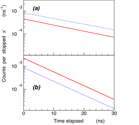
Figure 5: (Online color) Time evolutions of the total count rates of metastable $\pi{\rm{}^{4}He}^{+}$ that undergo $\pi^{-}$ nuclear absorption (solid lines) and $\pi^{-}\rightarrow\mu^{-}+\overline{\nu}_{\mu}$ decay (dotted lines), simulated for collisional deexcitation rates of (a) $\gamma_{\rm col1}=\gamma_{\rm col2}=0$, and (b) $8\times 10^{7}$ s^-1. The count rates are normalized to the total number of $\pi^{-}$ that come to rest in the helium target. Prompt nuclear absorptions of $\pi^{-}$ that occur at $t=0$ are not shown.

In Fig. 5 (a), the evolutions of $\Gamma_{\rm abs}(t)$ and $\Gamma_{\pi\rightarrow\mu}(t)$ are plotted for times $t=0-30$ ns in solid and dotted lines. The Auger and radiative decay rates are fixed to the theoretical values, while collisional deexcitations are neglected ($\gamma_{\rm col1}=\gamma_{\rm col2}=0$). The states $(17,16)$ and $(16,15)$ contain primary populations of $P_{(17,16)}(t=0)=0.005$ and $P_{(16,15)}(t=0)=0.018$, normalized to the total number of $\pi^{-}$ stopped in the helium target. The results of Fig. 5 (a) show that integrated populations of $\int_{0}^{\infty}\Gamma_{\rm abs}dt=0.007$ and $\int_{0}^{\infty}\Gamma_{\rm\pi\rightarrow\mu}dt=0.016$ respectively undergo nuclear absorption and $\pi^{-}\rightarrow\mu^{-}+\overline{\nu}_{\mu}$ decay, with mean cascade lifetimes of $\tau_{c}=16-18$ ns .

This disagrees with the results of experiments Nakamura et al. (1992) carried out using liquid-helium targets, which implies values of $\int_{0}^{\infty}\Gamma_{\rm abs}dt=0.017$, $\int_{0}^{\infty}\Gamma_{\rm\pi\rightarrow\mu}dt=0.006$, and $\tau_{c}\sim 7$ ns, i.e., most of the long-lived $\pi^{-}$ undergo nuclear absorption instead of $\pi^{-}\rightarrow\mu^{-}+\overline{\nu}_{\mu}$ decay. The 7-ns decay lifetime of the experimental spectra in Ref. Nakamura et al. (1992) cannot be reproduced by adjusting the primary populations $P_{(n,\ell)}(t=0)$ alone in our model, as the calculated decay rates in Fig. 1 appear to be too small.

The spectrum of Fig. 5 (b) was obtained by assuming collisional deexcitation rates of $\gamma_{\rm col1}\sim\gamma_{\rm col2}\sim 8\times 10^{7}$ s^-1. The other parameters are the same as those used in Fig. 5 (a). The mean cascade lifetime $\tau_{c}\sim 7$ ns and the populations $\int_{0}^{\infty}\Gamma_{\rm abs}dt=0.017$ and $\int_{0}^{\infty}\Gamma_{\rm\pi\rightarrow\mu}dt=0.006$ destroyed via the two channels now agree with the experimental results. This model is used in our simulation of the laser spectroscopic signal in the following sections.

V Laser spectroscopic method

V.1 Laser transitions

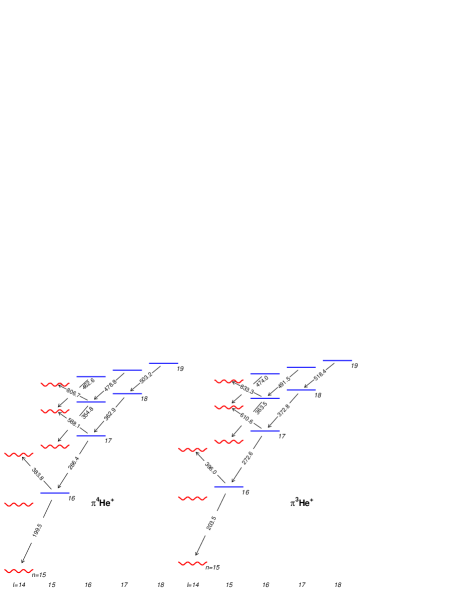
Figure 6: (Online color) Energy level diagram of $\pi{\rm{}^{4}He}^{+}$ and $\pi{\rm{}^{3}He}^{+}$ isotopes. Arrows indicate the laser transitions of the types $(n,\ell)\rightarrow(n-1,\ell-1)$ and $(n,\ell)\rightarrow(n+1,\ell-1)$. The transition wavelengths are shown in nanometers.

As mentioned earlier, we will excite laser transitions from the metastable $\pi{\rm He}^{+}$ states (indicated in Fig. 6 by solid lines) to the Auger-dominated short-lived states (wavy lines). The resonance condition between the laser and $\pi{\rm He}^{+}$ is revealed as a sharp spike in the rate of neutrons, protons, deuterons, and tritons that emerge (Sect. V.3) from the resulting $\pi^{-}$ absorption.

Fig. 6 and Table 3 show some $E1$ transition wavelengths and frequencies which include QED corrections. The strongest resonance signals are expected for the transitions $(n,\ell)=(16,15)$$\rightarrow$$(15,14)$, $(16,15)$$\rightarrow$$(17,14)$, and $(17,16)$$\rightarrow$$(18,15)$ in $\pi{\rm{}^{4}He^{+}}$, since the parent states presumably contain large populations (Sec. IV.1). The favored transition $(16,15)$$\rightarrow$$(15,14)$ has the largest transition amplitude, but laser light at the resonant wavelength of $199.5$ nm is difficult to generate. Laser beams of $383.8$ nm and 588.1 nm for the transitions $(16,15)$$\rightarrow$$(17,14)$ and $(17,16)$$\rightarrow$$(18,15)$ can be readily produced using Ti:sapphire or dye lasers.

The laser fluence $I$ needed to excite these transitions within the 7-ns lifetime of $\pi{\rm{}^{4}He}^{+}$ is roughly estimated in the following way. The transition matrix element of the single-photon transition $(v,L,J,M_{J})\rightarrow(v^{\prime},L^{\prime},J^{\prime},M_{J})$ from a substate of vibrational, orbital angular momentum, total angular momentum, and total azimuthal quantum numbers $v$, $L$, $J$, and $M_{J}$ induced by linearly-polarized laser light can be calculated using the Wigner 3-j and 6-j symbols as,

$$\kappa_{JJ^{\prime}M_{J}} = (-1)^{J-M_{J}}\left(\begin{array}[]{@{\,}ccc@{\,}}J&1&J^{\prime}\\ -M_{J}&0&M_{J}\\ \end{array}\right)$$ (23)

$$\times (-1)^{J+L^{\prime}-\frac{1}{2}}\sqrt{(2J+1)(2J^{\prime}+1)}\left\{\begin{array}[]{@{\,}ccc@{\,}}L^{\prime}&J^{\prime}&\frac{1}{2}\\ J&L&1\\ \end{array}\right\}$$ (26)

$$\times \langle L^{\prime}v^{\prime}\|\mathbf{\hat{d}}\|Lv\rangle.$$ (27)

This is related to the Rabi oscillation frequency $\Omega_{JJ^{\prime}M_{J}}/2\pi$ in atomic units induced by a linearly-polarized, resonant laser field of amplitude $F$ by,

$$\frac{\Omega_{JJ^{\prime}M_{J}}({\rm a.u.})}{2\pi}=\left|\kappa_{JJ^{\prime}M_{J}}\right|F$$ (28)

The $\pi{\rm{}^{4}He}^{+}$ primary populations are assumed to be uniformly distributed over the $\sim 60$ fine-structure and magnetic substates of the resonance parent state. The optical Bloch equations Hori et al. (2004); Hori and Korobov (2010) between pairs of states $(v,L,J,M_{J})$ and $(v^{\prime},L^{\prime},J^{\prime},M_{J})$ are then numerically integrated, and the results averaged over all substates.

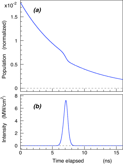
Figure 7: (Online color) (a) Population evolution of the $\pi{\rm{}^{4}He}^{+}$ state $(n,\ell)=(16,15)$ as a function of time elapsed. At $t=7$ ns, a 1-ns-long laser pulse excites the transition $(16,15)\rightarrow(17,14)$. This resulting in a sudden reduction of the population. (b) Temporal intensity profile of the laser pulse in MW cm^-2.

In Fig. 7 (a), the population evolution $P_{(16,15)}(t)$ of the state $(16,15)$ is plotted. At $t=7$ ns, a 1 ns-long resonant laser pulse of fluence $I\sim 6$ mJ cm^-2 and the temporal intensity profile shown in Fig. 7 (b) irradiates the atom and induces the transition $(16,15)\rightarrow(17,14)$. An abrupt $\varepsilon\sim 20\%$ reduction in $P_{(16,15)}(t)$ is seen, whereas the $\pi^{-}$ excited to $(17,14)$ undergoes Auger decay at a rate $A_{(17,14)}=1.7\times 10^{11}$ s^-1. A corresponding spike appears in the rate of $\pi^{-}$ absorptions, with an intensity of $\sim 10^{-3}$ normalized to the total number of $\pi^{-}$ which come to rest in the helium target at $t=0$. The simulation indicates that a fluence $I>30$ mJ cm^-2 can strongly saturate the transition and deplete most of the population in $(16,15)$. The high power requirement is due to the small transition amplitude, and the large Auger rate of $(17,14)$, which causes rapid dephasing in the laser-induced transition.

Lasers of pulse length $\sim 10$ ns and lower fluence $I\sim 1$ mJ cm^-2 can saturate the favored transition $(17,16)\rightarrow(16,15)$ at a wavelength of 266.4 nm between two metastable states. This alone would not produce a spike in the rate of $\pi^{-}$ absorption events, since our spectroscopy method relies on inducing a transition to an Auger-dominated state. A second laser with saturating fluence tuned to $(16,15)$$\rightarrow$$(17,14)$ or $(17,16)$$\rightarrow$$(18,15)$ is needed to detect the change in the $\pi^{-}$ population induced by the first 266.4-nm laser, in a two-step resonance configuration.

V.2 Resonance profile

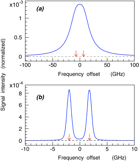
Figure 8: (Online color) Resonance profiles of the $\pi{\rm{}^{4}He}^{+}$ transitions (a) $(n,\ell)=(16,15)\rightarrow(17,14)$ and (b) $(17,16)\rightarrow(16,15)$. Note the different scales for the laser frequency offset. Arrows indicate the positions of the dominant fine structure sublines.

In Fig. 8 (a), the resonance profile of the $\pi{\rm{}^{4}He}^{+}$ transition $(16,15)\rightarrow(17,14)$ excited with a laser fluence $I\sim 6$ mJ cm^-2 is simulated. The intensity of the $\pi^{-}$ absorption spike implied by Fig. 7 is plotted as a function of the laser frequency $\Delta\nu$ detuned from the spin-independent resonance frequncy $\nu_{\rm exp}$. The width of this profile is predominantly caused by the contribution $A_{(17,14)}/2\pi\sim 26$ GHz of the Auger decay rate of the resonance daughter state and the spacing ($\sim 13.7$ GHz) between the fine structure sublines, the positions of which are indicated by arrows. It should in principle be possible to determine the centroid of this profile with a precision of $<1$ GHz. This corresponds to a fractional precision of better than $\sim 1\times 10^{-6}$ on $\nu_{\rm exp}$.

Narrower lines are seen for the favored transition $(17,16)\rightarrow(16,15)$ [Fig. 8 (b)] by using 266.4- and 383.8-nm laser pulses in sequence. The frequency of the former laser is scanned over the resonance, whereas the latter is fixed to the transition $(16,15)$$\rightarrow$$(17,14)$. This profile was simulated for a 10-ns-long laser pulse of $I\sim 0.1$ mJ cm^-2 for the 266.4-nm laser. The fine-structure sublines can now be resolved as distinct peaks. The 1-GHz widths of the peaks arises from the 7-ns-lifetime of $\pi{\rm He}^{+}$, power broadening effects, and the finite observation time. This implies that $\nu_{\rm exp}$ can in principle be determined to a precision of a few 10’s MHz, which corresponds to a fractional precision of $\sim 10^{-8}$.

V.3 Detection of $\pi^{-}$ absorption

Past experiments on the longevity of $\pi^{-}$ in helium targets Fetkovich and Pewitt (1963); Block et al. (1963, 1965); Zaĭmidoroga et al. (1967); Nakamura et al. (1992) used bubble chambers, multiwire proportional chambers, and sodium iodide spectrometers to identify the varieties and trajectories of the particles that emerged from the decay or nuclear absorption of $\pi^{-}$. This helped to isolate the signal electrons, $\mu^{-}$, or protons from background events. These techniques were optimized for low- to moderate count rates. A laser spectroscopy experiment of $\pi{\rm He}^{+}$, on the other hand, would need $\pi^{-}$ beam intensities and detection efficiencies which are $>2$ orders of magnitude higher, in order to resolve the resonance signal. We intend to achieve this by detecting the signal neutrons, protons, deuterons, and tritons using plastic scintillation counters Sótér et al. (2014) surrounding the experimental target, which do not have particle identification, or vertex reconstruction, capabilities.

The $\pi^{-}$ absorption into the ${\rm{}^{4}He}$ nucleus predominantly leads to one of four final states Schiff et al. (1961); Eckstein (1963); Ziock et al. (1970); Barrett et al. (1973); Kubodera (1975); Cernigoi et al. (1981); Daum et al. (1995); Bistirlich et al. (1970); Baer et al. (1977),

$$\pi^{-}+{\rm{}^{4}He} \rightarrow {\rm{}^{3}H}+n+118.5\ {\rm MeV},$$ (29)

$$\rightarrow {\rm{}^{2}H}+n+n+112.2\ {\rm MeV},$$ (30)

$$\rightarrow \ \ p+n+n+n+110.0\ {\rm MeV},$$ (31)

$$\rightarrow {\rm{}^{4}H^{\ast}}+\gamma.$$ (32)

Their measured branching ratios Daum et al. (1995); Bistirlich et al. (1970); Baer et al. (1977) are respectively, $(17\pm 9)\%$, $(63\pm 26)\%$, $(21\pm 16)\%$, and $\sim 1.5\%$.

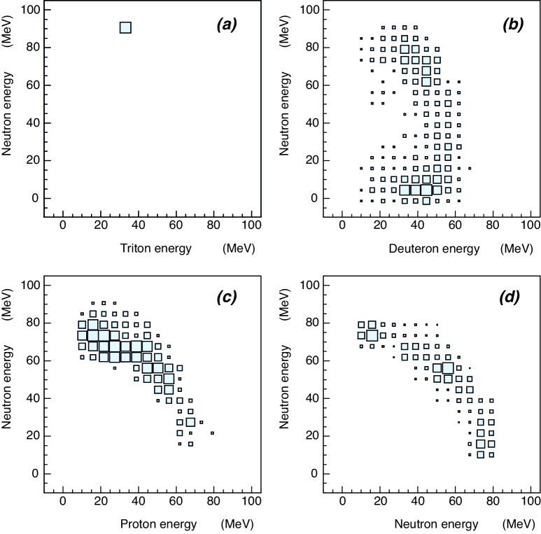
Figure 9: (Online color) Correlations of the kinetic energies of (a) triton-neutron, (b) deuteron-neutron, (c) proton-neutron, and (d) neutron-neutron pairs which emerge from $\pi^{-}$ absorption into a ⁴He nucleus (see the text). The primary energies of the particles before they slow down in the experimental apparatus are shown. They are based on the experiments of Refs. Ziock et al. (1970); Barrett et al. (1973); Cernigoi et al. (1981); Daum et al. (1995), which are augmented by theoretical distributions Eckstein (1963); Kubodera (1975) for the regions where experimental data is not available. The $E\leq 10$ MeV charged particles are ignored. Some of the details of these plots may be inaccurate, but they are sufficient to roughly simulate the intensity of the $\pi^{-}$ absorption signal in the $\pi{\rm{}^{4}He}^{+}$ laser spectroscopy experiment.

Figs. 9 (a)–(c) show the correlations of the kinetic energies between triton-neutron, deuteron-neutron, and proton-neutron pairs that emerge in the non-radiative channels of Eqs. 29, 30, and 31, respectively. Fig. 9 (d) shows the neutron-neutron pairs which originate from the channels of Eqs. 30 and 31 added together. All these particles tend to emerge collinearly Daum et al. (1995). The plots are based on the experiments of Refs. Ziock et al. (1970); Barrett et al. (1973); Cernigoi et al. (1981); Daum et al. (1995), which are augmented by theoretical distributions Eckstein (1963); Kubodera (1975) for regions where experimental data are not available. The $E\leq 10$ MeV charged particles are ignored. Some details of these plots may be inaccurate, but they are sufficient to roughly simulate the $\pi{\rm He}^{+}$ signal.

In the two-body channel of Eq. 29, a monoenergetic triton and neutron of energies $E_{t}=30.6$ MeV and $E_{n}=90$ MeV [Fig. 9 (a)] emerge back to back. The energy distribution [Fig. 9 (b)] of the three-body channel of Eq. 30 has been interpreted by several groups in the following way Kubodera (1975); Daum et al. (1995). Due to final-state interaction effects, the spectrum contains a strong peak corresponding to a $E_{d}\sim 56$ MeV deuteron, which is accompanied by two collinear $E_{n}\sim 28$-MeV neutrons emitted in the opposite direction. The two maxima of Fig. 9 (b) at positions of $(E_{d},E_{n})\sim(40{\rm\ MeV},70{\rm\ MeV})$ and $(40{\rm\ MeV},0{\rm\ MeV})$ correspond to the so-called “quasi-free” absorption of $\pi^{-}$. This leads to the deuteron and a neutron emitted nearly back-to-back, while the remaining neutron plays the role of a spectator of low energy. The peak at $E_{n}=56$ MeV in the neutron spectrum of Fig. 9 (d) represents the quasi-free absorption of $\pi^{-}$ into a proton-neutron pair within the nucleus; this results in the emission of two back-to-back neutrons and a spectator deuteron. The minimum near the center of the truncated ellipse of Fig. 9 (b) at $(E_{d},E_{n})\sim(30{\rm\ MeV},40{\rm\ MeV})$ is the unlikely case where the three particles emerge in a non-collinear way, with momenta which are uniformly distributed in phase space.

The energy distribution of the protons in the four-body channel of Eq. 31 extends up to $E_{p}\sim 70$ MeV and is skewed towards lower energies [Fig. 9 (c)]. The quasi-free absorption of the $\pi^{-}$ into a proton-proton pair within the nucleus can lead to the back-to-back emission of a proton and a neutron of $E_{n}\sim E_{p}\sim 56$ MeV. The measured branching ratio of this process is small $(3\pm 1)\%$ Daum et al. (1995).

Equation 32 describes those $\pi^{-}$ that occupy the low-$n_{i}$ ionic states of $\pi{\rm He}^{2+}$, that subsequently undergo radiative capture Bistirlich et al. (1970); Baer et al. (1977) into ${}^{4}{\rm He}$ nuclei. The energy spectrum of the emitted $\gamma$-rays has a maximum at $E_{\gamma}\sim 112$ MeV. Its shape implies the excitations of several resonance states of the ${\rm{}^{4}H}$ nucleus, at energies of $E=3.4$–7.4 MeV relative to the ${\rm{}^{3}H}+n$ decay threshold. Low-energy neutrons are subsequently emitted.

The final states for $\pi^{-}$ absorption into the ${\rm{}^{3}He}$ nucleus Truöl et al. (1974); Backenstoss et al. (1986); Corriveau et al. (1987); Gotta et al. (1995) are predominantly,

$$\pi^{-}+{\rm{}^{3}He} \rightarrow {\rm{}^{2}H}+n,$$ (33)

$$\rightarrow \ \ p+n+n,$$ (34)

$$\rightarrow {\rm{}^{3}H}+\gamma,$$ (35)

$$\rightarrow {\rm{}^{2}H}+n+\gamma,$$ (36)

$$\rightarrow \ \ p+n+n+\gamma,$$ (37)

$$\rightarrow {\rm{}^{3}H}+\pi^{0}.$$ (38)

The experimental branching ratios are respectively $(16\pm 2)\%$, $(58\pm 5)\%$, $(5.7\pm 0.2)\%$, $(3.6\pm 1.2)\%$, $(3.6\pm 1.3)\%$, and $(15\pm 0.6)\%$ Corriveau et al. (1987); Gotta et al. (1995). The nonradiative nuclear absorptions of Eqs. 33 and 34 are expected to produce the strongest signals in the $\pi{\rm{}^{3}He}^{+}$ experiment. The former results in the back-to-back emission of a monoenergetic deuteron and a neutron of $E_{d}\sim 45$ MeV and $E_{n}\sim 90$ MeV Gotta et al. (1995). The protons and neutrons in the three-body channel of Eq. 34 are distributed up to $>90$ MeV and tend to emerge collinearly. Unlike the ${\rm{}^{4}He}$ case, there are significant contributions from radiative nuclear capture (Eqs. 35–37) and charge-exchange (Eq. 38) processes between the $\pi^{-}$ and ${\rm{}^{3}He}$ nucleus.

When $\pi^{-}$ are allowed to come to rest in thick ${\rm{}^{4}He}$ targets, some of the secondary protons, deuterons, and tritons slow down and stop in the helium. This reduces the efficiency $D$ of the scintillation counters detecting the $\pi^{-}$ absorption. The experiment of Ref. Nakamura et al. (1992), for example, counted the $E_{p}>50$-MeV protons which emerged from a liquid helium target of diameter $d=230$ mm. This provided a clean signal for delayed $\pi^{-}$ events with a high degree of background elimination, but we estimate the corresponding $D$-value to be $<1\%$. This efficiency can be increased by (i) using a small ($d<40$ mm) helium target which allows protons, deuterons, and some tritons of $E_{p}\geq 20$ MeV, $E_{d}\geq 30$ MeV, and $E_{t}=30.6$ MeV to emerge from it and (ii) detecting the neutrons that are produced at an order-of-magnitude higher rate than the protons. A plastic scintillation counter of thickness $t_{r}\sim 40$ mm can detect $E_{n}=10$-, 40-, and 80-MeV neutrons with efficiencies of $\sim 10\%$, $\sim 5\%$, and $\sim 3\%$, respectively Abdel-Wahab et al. (1982).

V.4 Coincidences and event rates

The arrival of the laser pulses at the experimental target must coincide with the formation of $\pi{\rm He}^{+}$, if any transition is to be induced. This is difficult to achieve since the $\pi{\rm He}^{+}$ decays within tens of nanoseconds, whereas the arrival time of individual $\pi^{-}$ produced in synchrotron facilities cannot easily be predicted with nanosecond-scale precision. Past experiments on $\overline{p}{\rm He}^{+}$ Morita et al. (1994); Hori et al. (2004) or muonic hydrogen atoms Pohl et al. (2010) first detected the formation of the exotic atoms and then triggered some pulsed lasers to irradiate them at a time $t=1$–10 $\mu{\rm s}$ after formation. In the $\pi{\rm He}^{+}$ case, the detected atoms would decay well before the laser pulses could reach them. Another method for $\overline{p}{\rm He}^{+}$ spectroscopy Hori et al. (2004, 2011) involved ejecting a 200-ns-long pulsed beam containing $>10^{7}$ antiprotons from a synchrotron and triggering the laser so that a single laser pulse arrived at the target with a $t=1$–10 $\mu{\rm s}$ delay, relative to the antiprotons. A bright 200-ns-long flash caused by the antiprotons that promptly annihilated in the helium was detected, followed by a much longer but less intense tail from the delayed annihilations of the metastable $\overline{p}{\rm He}^{+}$. The laser resonance signal was superimposed on this tail. This method is also difficult to apply to $\pi{\rm He}^{+}$, which would be destroyed well within the initial flash of nuclear absorptions that occurs during the arrival of a 200-ns-long $\pi^{-}$ beam.

We instead propose synchronization of the laser pulses to the $\pi^{-}$ beam of the PSI cyclotron Wagner et al. (2009). Here radiofrequency cavities excited at $f_{c}=50.63$ MHz arrange the protons into 0.3-ns-long bunches at intervals of $f_{c}^{-1}=19.75$ ns, and accelerate them to a kinetic energy of $E=590$ MeV. The protons are then allowed to collide with a 40-mm-thick carbon target, thereby producing the $\pi^{-}$. A magnetic beamline Adam et al. (2013) collects the $\pi^{-}$ of a certain momentum, and transports them over $\sim 15$ m to the position of the experimental helium target. The $\pi^{-}$ thus arrive as a train of bunches that are synchronized to $f_{c}$. This signal triggers the laser, so that the laser pulse arrives $t=7$ ns after a $\pi^{-}$ bunch. Most of the laser pulses will irradiate an “empty” target, since the $\sim 98\%$ majority of the $\pi^{-}$ are absorbed promptly without forming metastable atoms Nakamura et al. (1992). A high $\pi^{-}$ beam intensity of $N_{\pi}>f_{c}=5\times 10^{7}$ s^-1 is needed to ensure a sufficient ($>0.1\%$) probability of coincidence between the laser pulses and $\pi{\rm He}^{+}$ populating the resonance parent state.

The rate of detecting $\pi^{-}$ absorption events which signal the laser transition can then be estimated as

$$\Gamma_{\rm evt}\sim\varepsilon DN_{\pi}S_{\pi}P_{(n,\ell)}f_{\rm las}f_{c}^{-1}.$$ (39)

According to the simulation of Sec. VI.1, $S_{\pi}>50\%$ of the incoming $\pi^{-}$ come to rest in a 20-mm-diam volume of the helium target. This volume is then irradiated by a resonant laser beam of repetition rate $f_{\rm las}\sim$ 0.1–1 kHz. Only the data from $\pi^{-}$ bunches that coincide with the laser are acquired at a rate $f_{\rm las}$, whereas the remaining bunches of rate $f_{c}-f_{\rm las}$ are ignored. Among these $\pi^{-}$, the fraction that occupies the resonance parent state at the moment of laser irradiation is assumed in Sect. IV.4 and Fig. 7 to be $P_{(16,15)}(t=7{\ \rm ns})\sim 0.007$. The efficiency of the laser depopulating the parent state is estimated in Sect. V.1 to be $\varepsilon\sim 20\%$. The resulting $\pi^{-}$ absorptions are detected by the scintillation counters with a typical efficiency of $D\sim 20\%$. A $\pi^{-}$ beam intensity of $N_{\pi}\sim 10^{8}$ s^-1 would therefore imply $\Gamma_{\rm evt}\sim 100-1000$ h^-1.

VI Monte-Carlo simulations

VI.1 Stopping of $\pi^{-}$ in helium

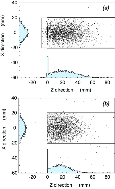
Figure 10: (Online color) (a) Simulated spatial distribution of $\pi^{-}$ with momentum 80 MeV/c and momentum spread $\sim 8\%$ coming to rest in a liquid-helium target. A two-dimensional projection, and $x$ and $z$ projections of the $\pi^{-}$ distributions are shown superimposed. The $\pi^{-}$ arrive from the left side of the diagram and traverse an 8-mm-thick aluminum degrader foil before entering the 40-mm-diameter target at position $z=0$. The outlines of the foil and target chamber are indicated by solid lines. (b) Spatial stopping distribution of 40-MeV/c $\pi^{-}$ beam, coming to rest in a helium gas target of pressure $p\sim 1.7\times 10^{5}$ Pa and temperature $T\sim 6$ K (b).

The $\pi^{-}$ must come to rest in the helium target with a high efficiency, to maximize the produce yield of $\pi{\rm He}^{+}$. The $\pi$E5 beamline of PSI Adam et al. (2013) provides a $\pi^{-}$ beam of intensity $N_{\pi}\sim 10^{8}$ s^-1, momentum $\sim 80$ MeV/c, momentum spread $\sim 8\%$, and diameter $d\sim 20$ mm. Figure 10 (a) shows the simulated spatial distribution of the $\pi^{-}$ coming to rest in a $40$-mm-diameter, 100-mm-long cylindrical chamber filled with liquid helium of atomic density $\rho\sim 2\times 10^{22}$ cm^-3. The slowing down of the $\pi^{-}$ is simulated using the multiple scattering effect according to the Molière distribution, and the energy straggling effect according to the Vavilov distribution. The $\pi^{-}$ traverse an aluminum degrader plate before entering the helium target; by carefully adjusting the degrader thickness to $t_{r}\sim 8$ mm, some $S_{\pi}>50\%$ of the $\pi^{-}$ are stopped within a 20-mm-diameter, 50-mm-long cylindrical region along the beam axis. The small size of this stopping distribution ensures a high timing resolution and detection efficiency for $\pi^{-}$ absorption. It also allows the $\pi{\rm He}^{+}$ produced in this volume to be readily irradiated with high-intensity laser light, fired into the target in an anticollinear direction with the $\pi^{-}$ beam, as in the experimental setups of Refs. Hori et al. (2001, 2004).

Beams of lower momentum $\pi^{-}$ can be efficiently stopped in a helium-gas target, where collisional quenching, broadening, and shifting of the $\pi{\rm He}^{+}$ resonance lines may be reduced. Fig. 10 (b) shows the spatial distribution of $\pi^{-}$ with a momentum of 40 MeV/c which come to rest in a gas target of pressure $p\sim 1.7\times 10^{5}$ Pa and temperature $T\sim 6$ K. This corresponds to a density $\rho\sim 2.6\times 10^{21}$ cm^-3. The intensity of such a beam is limited to $N_{\pi}\leq 10^{6}$ s^-1, due to the lower $\pi^{-}$ production yield, and the fact that most of the slow $\pi^{-}$ decay in-flight before they can reach the helium target. This implies a signal rate $\Gamma_{\rm evt}\sim 1-10$ h^-1 according to Eq. 39.

VI.2 Backgrounds

The experiment has several background sources:

Prompt absorption, the 98$\%$ majority of the $\pi^{-}$ that come to rest in the helium target undergo nuclear absorption within picoseconds (Sect. V.3). The flux of neutrons and charged particles produced by this is $>10^{3}$ times larger than the laser spectroscopic signal of $\pi{\rm He}^{+}$. The signal can be isolated from this background, by adjusting the laser pulse to arrive $t\sim 7$ ns after the $\pi^{-}$ (see Fig. 7).

Cascade of $\pi{\rm He}^{+}$, only a small fraction of the metastable $\pi{\rm He}^{+}$ will undergo laser excitation. The remaining atoms will decay spontaneously, and produce a continuous background in the measured time spectrum.

Electron contamination, the $\pi^{-}$ beam is contaminated with electrons of intensity $N_{e}\sim 10^{9}$ s^-1. These electrons can scatter off the experimental target and produce background in the surrounding scintillation counters. The contamination can be reduced to $N_{e}\sim 10^{7}$ s^-1 by using a $E\times B$ separator positioned upstream of the target.

Muon contamination, the beam also contains contaminant $\mu^{-}$ with a ratio $N_{\mu}/N_{\pi}\sim 1$, depending on the momentum and flight path of the $\pi^{-}$. Some of the $\mu^{-}$ come to rest in the helium target and produce muonic helium atoms. Most of these undergo $\mu^{-}\rightarrow e^{-}+\overline{\nu}_{e}+\nu_{\mu}$ decay into an electron, an electron-based antineutrino, and a muon-based neutrino with a partial decay rate of $\gamma_{\mu}\sim 4.5\times 10^{5}$ s^-1. The electrons of mean energy $E\sim 40$ MeV can be isolated to some extent from the signal neutrons, protons, deuterons, and tritons by their smaller energy loss in the scintillation counters Beringer et al. (2012). The competing process of $\mu^{-}$ capture into the nucleus via weak interaction,

$$\mu^{-}+{\rm{}^{4}He}\rightarrow{\rm{}^{3}H}+n+\nu_{\mu},$$ (40)

has a small capture rate $\gamma_{\rm cap}=300$–400 s^-1 Measday (2001), so that the emerging neutrons do not constitute a significant background. The $\mu^{-}$ that stop in the metallic walls of the target chamber are captured into heavier nuclei at a higher rate $\gamma_{\rm cap}>7\times 10^{4}$ s^-1 Measday (2001). This results in the emission of 0.1–0.2 neutron of energy $E_{n}\geq 10$ MeV per stopped $\mu^{-}$ Measday (2001). Since most of these neutrons are of $E_{n}<20$ MeV, this background can be reduced by rejecting those events with a small energy deposition in the scintillation counters.

VI.3 Signal-to-background ratios

The signal-to-background ratio of the laser resonance depends on the design of the experimental apparatus, the characteristics of the $\pi^{-}$ and laser beams, the populations in the $\pi{\rm He}^{+}$ states, and the data analysis methods. We carried out Monte-Carlo simulations using the GEANT4 toolkit Agostinelli et al. (2003), to roughly estimate the signal-to-background ratio for an apparatus that is conceptually similar to those of Refs. Hori et al. (2001, 2004). The $\pi^{-}$ beam of momentum 80 MeV/c came to rest in a liquid-helium target (Sec. VI.1) at intervals of $f_{c}^{-1}=19.75$ ns. The beam contained contaminant electrons and $\mu^{-}$ with ratios of $N_{e}/N_{\pi}=0.2$ and $N_{\mu}/N_{\pi}=1$. Some $1.6\%$ and $0.7\%$ of the $\pi^{-}$ (Sec. IV.4) were respectively captured into the $\pi{\rm He}^{+}$ states $(n,\ell)=(16,15)$ and $(17,16)$. These atoms decayed with a mean lifetime of $\tau_{c}\sim 7$ ns. The laser transition $(16,15)$$\rightarrow$$(17,14)$ induced at $t=7$ ns depopulated $\varepsilon\sim 20\%$ of the $\pi^{-}$ that occupied $(16,15)$ (Sect. V.1). Neutrons, protons, deuterons, and tritons emerged from the resulting $\pi^{-}$ absorption with the branching ratios and energy distributions described in Sect. V.3. For simplification, we simulated only the two highest-energy particles in each event of Eqs. 30 and 31. Due to the dominant nature of the quasi-free absorption Daum et al. (1995), we assume that the remaining particles tend to have low energies and would not strongly contribute to the $\pi{\rm He}^{+}$ signal. Some of these signal particles traversed the 1.4-mm-thick lateral walls of the target chamber (Fig. 10) made of aluminium. They were detected by an array of 40-mm-thick plastic scintillation counters (Sect. V.3), which covered a solid angle of $\sim 2\pi$ steradians seen from the target. The trajectories of the particles were followed for $\sim 100$ ns.

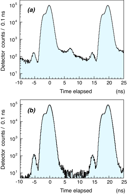
Figure 11: (Online color) (a) Simulated time spectrum of metastable $\pi{\rm{}^{4}He}^{+}$. The time elapsed from $\pi^{-}$ arrival at a liquid helium target, until a particle hit was registered in an array of plastic scintillation counters surrounding the target is shown (see the text). The $\pi^{-}$ arrive at intervals of $f_{c}^{-1}=19.75$ ns, synchronized to the acceleration frequency $f_{c}$ of the PSI cyclotron. The laser resonance transition $(n,\ell)=(16,15)\rightarrow(17,14)$ is induced at $t=7$ ns. The resulting peak in the rate of particle hits is visible over the background arising from the spontaneous decay of $\pi{\rm{}^{4}He}^{+}$. (b) Time spectrum obtained by assuming that all the $\pi^{-}$ are promptly absorbed in the helium target, without forming metastable $\pi{\rm{}^{4}He}^{+}$.

Fig. 11 (a) shows the spectrum of time elapsed from $\pi^{-}$ arrival at the experimental target, until a hit was registered in the scintillation counters. It represents $10^{7}$ $\pi^{-}$ arrivals coinciding with the laser pulse. Some of the background electrons and neutrons were rejected by accepting only those events that deposited more than $E_{\rm cut}=10$ MeV of energy in the counters. No other particle identification or vertex reconstruction was carried out. The peaks at $t=0$ and $19.75$ ns correspond to arrivals of $\pi^{-}$ which undergo prompt nuclear absorption. The secondary peaks at $t=-2$ and $18$ ns represent $\pi^{-}$ that stop in the upstream walls of the target chamber. Those at $t=-5.5$ and $14.5$ ns are caused by the electrons that scatter off the target and strike the scintillation counters. All these peaks are broadened due to the finite timing resolution of the scintillation counters which was assumed to be $\sim 1$ ns and the time-of-flight of the particles in the experimental apparatus.

The spontaneous deexcitations of metastable $\pi{\rm He}^{+}$ give rise to the continuous spectrum which decays with a lifetime of $\tau_{c}=7$ ns. The peak at $t=7$ ns with a signal-to-background ratio of $\sim 2$ corresponds to the laser resonance. The intensity of this signal peak is linearly dependent on the population $P_{(16,15)}(t)$ of the parent state, and the $\varepsilon$-value of the laser (Sect. V.1). The spectrum represents $\sim 30$ h of data taking at the experimental conditions of Sect. V.4; it may therefore take a few months to repeat the measurements at 20–30 settings of the laser frequency around the $\pi{\rm He}^{+}$ resonance, and obtain the spectral profile of Fig. 8 needed to determine $\nu_{\rm exp}$.

Fig. 11 (b) shows the time spectrum obtained by assuming that all the $\pi^{-}$ are promptly absorbed in the helium without forming metastable $\pi{\rm He}^{+}$. This spectrum represents the sum of all the background processes of Sect. VI.2. Its intensity critically depends on the design of the target and scintillation counters, and the $E_{\rm cut}$-value used to reject the minimum-ionizing electrons that emerge from, e.g., $\mu^{-}\rightarrow e^{-}+\overline{\nu}_{e}+\nu_{\mu}$ decay. These must be carefully optimized in the actual experiment.

VII Discussions and Conclusions

We have carried out three-body QED calculations on the spin-independent energies, fine structure, $E1$ transition frequencies, and Auger and radiative rates of metastable $\pi{\rm{}^{3}He}^{+}$ and $\pi{\rm{}^{4}He}^{+}$ atoms in the region $n=15$–19. We described a method for laser spectroscopy, in which pulsed lasers induce transitions from the metastable states, to states with picosecond-scale lifetimes against Auger decay. The Rydberg $\pi{\rm He}^{2+}$ ion that remains after Auger emission is rapidly destroyed in collisions with helium atoms. Here the ionic states undergo Stark mixing with $s$, $p$, and $d$ states, which leads to $\pi^{-}$ absorption into the helium nucleus. This results in a spike in the rates of neutrons, protons, deuterons, and tritons which emerge with kinetic energies up to 30–90 MeV. This signals the resonance condition between the laser and $\pi{\rm He}^{+}$. The feasibility of this experiment depends on the population of $\pi{\rm He}^{+}$ that occupies the resonance parent state. Based on the experimental work on $\overline{p}{\rm He}^{+}$, we assume that most of the metastable population lies in the states $(n,\ell)=(16,15)$ and $(17,16)$. We found that a cascade model which includes assumptions on collisional deexcitation rates, can reproduce the features of past experimental data Nakamura et al. (1992) on the lifetime of $\pi^{-}$ in liquid helium targets. Several candidate transitions, e.g., $(16,15)\rightarrow(17,14)$, appear to be amenable for detection. Although the decay and nuclear absorption of $\pi^{-}$ and $\mu^{-}$ give rise to several experimental backgrounds, Monte-Carlo simulations suggest that a spectroscopic signal can be resolved, if appropriate particle detection techniques were used. The PiHe collaboration now attempts to carry out this measurement using the PSI ring cyclotron facility. The experiment involves allowing a $\pi^{-}$ beam of intensity $>10^{8}$ s^-1 to come to rest in a helium target. The time structure of the beam will be used to synchronize the formation of $\pi{\rm He}^{+}$ in the target, with the arrival of resonant laser beams of fluence 0.1–10 mJ$\cdot$cm^-2. This may allow the transition frequencies of $\pi{\rm He}^{+}$ to be determined with a fractional precision of $10^{-8}-10^{-6}$ provided that the systematic uncertainties can be controlled.

Several effects can prevent the detection of the laser resonance signal, beyond those evaluated in this paper. Experiments on $\overline{p}{\rm He}^{+}$ have shown that some states become short-lived to nanosecond- and picosecond-scale lifetimes when the density of the helium target is increased Hori et al. (1998a, b, 2001, 2004). Collisions between $\overline{p}{\rm He}^{+}$ and normal helium atoms broadened and weakened some laser resonances, so that they could no longer be detected .

The mass $M_{\pi^{-}}$ of the $\pi^{-}$ can be determined by comparing the measured frequencies $\nu_{\rm exp}$ of $\pi{\rm He}^{+}$ with the results of the three-body QED calculations $\nu_{\rm th}$ described in this paper. The precision on $M_{\pi^{-}}$ will be ultimately limited by the finite lifetime $\tau_{\pi}\sim 26$ ns of $\pi^{-}$ according to the expression, $\left(2\pi\tau_{\pi}\nu_{\rm exp}\theta\right)^{-1}$, since this determines the relative natural width of the resonance compared to its energy. Here $\theta=1$–9 denotes the sensitivity of $\nu_{\rm th}$ on $M_{\pi^{-}}$. When $M_{\pi^{-}}$ was increased by 1 part per billion (ppb) in our three-body calculations, the $\nu_{\rm th}$ values for the $\pi{\rm{}^{4}He}^{+}$ transitions $(17,16)\rightarrow(16,15)$ and $(16,15)\rightarrow(17,14)$, and the $\pi{\rm{}^{3}He}^{+}$ transitions $(17,16)\rightarrow(16,15)$ and $(16,15)\rightarrow(17,14)$ were found to shift by $1.9$, $-1.1$, $1.9$, and $-9$ ppb, respectively Korobov (2006, 2008). The last of these transitions appears to be particularly sensitive to $M_{\pi^{-}}$. This implies that a fractional precision on $M_{\pi^{-}}$ of $<10^{-8}$ can in principle be achieved, as in the case of $\overline{p}{\rm He}^{+}$ Hori et al. (2011, 2006). In practice, systematic effects such as the shift and broadening of the resonance line due to atomic collisions Hori et al. (2001); Bakalov et al. (2000); Adamczak and Bakalov (2013); Kobayashi et al. (2013) in the experimental target, AC Stark shifts Hori and Korobov (2010), frequency chirp in the laser beam Hori and Dax (2009), and the statistical uncertainties due to the small number of detected events can prevent the experiment from achieving this precision. The lifetimes of some $\pi{\rm He}^{+}$ states may be shorter than $\tau_{\pi}$, due to collisional effects (Sects. IV.4 and V.2).

Past values of $M_{\pi^{-}}$ have been determined Beringer et al. (2012) in two ways, i): the X-ray transition energies of $\pi^{-}$ atoms were measured, and the results compared with relativistic bound-state calculations Marushenko et al. (1976); Carter et al. (1976); Lu et al. (1980); Jeckelmann et al. (1986, 1994); Lenz et al. (1998), or ii): the recoil momentum $p_{\mu^{+}}=29.79200(11)$ MeV/c Abela et al. (1984); Daum et al. (1991); Assamagan et al. (1994, 1996) of the positively-charged muon $\mu^{+}$ which emerges from a stationary, positively-charged pion undergoing $\pi^{+}\rightarrow\mu^{+}+\nu_{\mu}$ decay was precisely measured. The relativistic kinematical formula,

$$p_{\mu^{+}}^{2}+m_{\mu^{+}}^{2}=\left(M_{\pi^{+}}^{2}+m_{\mu^{+}}^{2}-m^{2}_{\nu_{\mu}}\right)^{2}/4M_{\pi^{+}},$$ (41)

was employed to determine the mass $M_{\pi^{+}}$ of the $\pi^{+}$, which according to CPT symmetry is equivalent to $M_{\pi^{-}}$. The mass $m_{\mu^{+}}$ of the $\mu^{+}$ was determined to a fractional precision of $4\times 10^{-8}$ from the results of microwave spectroscopy of the ground-state hyperfine structure of muonium atoms Liu et al. (1999); the $\nu_{\mu}$ was assumed to be very light ($m_{\nu_{\mu}}\sim 0$). The X-ray spectroscopy measurements are conventionally Beringer et al. (2012) treated as direct laboratory determinations of $M_{\pi^{-}}$, as they involve no such assumption on $m_{\nu_{\mu}}$.

The $M_{\pi^{-}}$ value with the highest fractional precision of $\sim 3\times 10^{-6}$ was obtained from measurements of the 4f–3d transition energy of $\pi{\rm{}^{24}Mg}$ atoms Jeckelmann et al. (1986, 1994); Beringer et al. (2012). The results of these experiments have shown a bifurcation, i.e., two groups of results near 139.570 and 139.568 MeV/$c^{2}$ Beringer et al. (2012) which arise from different assumptions on the electrons occupying the K-shell of the atom during X-ray emission. Ref. Beringer et al. (2012) notes that although the two solutions are equally probable, they chose the higher $M_{\pi^{-}}$ value which is consistent with a positive mass-squared value for $\nu_{\mu}$, i.e., $m^{2}_{\nu_{\mu}}>0$, according to Eq. 41. The lower $M_{\pi^{-}}$ value would result in a so-called tachionic solution $m^{2}_{\nu_{\mu}}<0$. A separate spectroscopy measurement on the 5g–4f transition in $\pi{\rm N}$ atoms Lenz et al. (1998) which did not suffer from the ambiguity on the electron shell occupancy, determined $M_{\pi^{-}}$ with a factor $\sim 1.5$ lower precision; the result was consistent with the higher $M_{\pi^{-}}$ value.

The present limit Beringer et al. (2012) on the $\nu_{\mu}$ mass obtained from direct laboratory measurements is $m_{\nu_{\mu}}<190$ keV/$c^{2}$ with a confidence level of 90$\%$. This result was obtained by combining the $\pi^{-}$ and $\mu^{+}$ masses determined by the above spectroscopy experiments on exotic atoms, the recoil momentum $p_{\mu^{+}}$ Abela et al. (1984); Daum et al. (1991); Assamagan et al. (1994, 1996), and Eq. 41. Although cosmological observations and neutrino oscillation experiments have established a much better limit of $\Sigma m_{\nu}<0.2-0.4$ eV/$c^{2}$ for the sum of the masses of stable Dirac neutrinos Beringer et al. (2012), this still represents the best limit obtained from direct laboratory measurements. By improving the experimental precision on $M_{\pi^{-}}$, the direct limit on $m_{\nu_{\mu}}$ can be improved by a factor $\sim 2$. Further progress would require a higher-precision measurement of $p_{\mu^{+}}$ using, e.g., the muon $g$-2 storage ring of Fermilab Carey et al. (2000).

Appendix A Relativistic and radiative corrections

We briefly describe the relativistic and radiative corrections in our calculations. Since we aim for $\sim 7$ significant digits of precision on the $\pi{\rm He}^{+}$ energy, recoil effects may be neglected. Atomic units are used.

The leading $R_{\infty}\alpha^{2}$-order relativistic contribution of the bound electron in the field of two massive particles can be expressed as Bethe and Salpeter (1977),

$$E_{rc}=\alpha^{2}\left\langle-\frac{\mathbf{p}_{e}^{4}}{8m_{e}^{3}}+\frac{1+2a_{e}}{8m_{e}^{2}}\left[Z_{\rm He}4\pi\delta(\mathbf{r}_{\rm He})+Z_{\pi}4\pi\delta(\mathbf{r}_{\pi})\right]\right\rangle.$$ (42)

Here $a_{e}=1.1596522\times 10^{-3}$ denotes the anomalous magnetic moment of the electron. The expectation values of the operators ${\bf p}^{4}_{e}$, $\delta({\bf r}_{{}_{\rm He}})$, and $\delta({\bf r}_{\pi})$ for $\pi{\rm{}^{4}He}^{+}$ and $\pi{\rm{}^{3}He}^{+}$ states are shown in Tables 1 and 2.

The next largest contribution is the one-loop self-energy of order $R_{\infty}\alpha^{3}$,

$$E_{se}^{(3)} = \alpha^{3}\frac{4}{3}\left[\ln{\frac{1}{\alpha^{2}}}-\beta(L,v)+\frac{5}{6}-\frac{3}{8}\right]$$ (43)

$$\times \left\langle Z_{\rm He}\delta(\mathbf{r}_{\rm He})+Z_{\pi}\delta(\mathbf{r}_{\pi})\right\rangle,$$

where $\beta(L,v)$ denotes the Bethe logarithm of the mean excitation energy due to emission and re-absorbtion of a virtual photon Bethe and Salpeter (1977); Korobov et al. (2013); Korobov (2014). We used the adiabatic effective potential $\beta_{nr}(R)$ (see Fig. 4 in Ref. Korobov et al. (2013)) for the two-center problem with Coulomb charges $Z_{1}=2$, $Z_{2}=-1$, which was averaged over the vibrational wave function $\chi_{L,v}(R)$ of a particular state. We also included the one-loop vacuum polarization using the expression,

$$E_{vp}^{(3)}=\frac{4\alpha^{3}}{3}\left[-\frac{1}{5}\right]\Bigl{\langle}Z_{\rm He}\delta(\mathbf{r}_{\rm He})+Z_{\pi}\delta(\mathbf{r}_{\pi})\Bigr{\rangle}.$$ (44)

Table 1: Nonrelativistic energies $E_{nr}$, Auger widths $\Gamma$, expectation values of operators ${\bf p}^{4}_{e}$, $\delta({\bf r}_{{}_{\rm He}})$, and $\delta({\bf r}_{\pi})$, and coefficients of the fine structure effective Hamiltonian $E_{1}$ for the $\pi{\rm{}^{4}He^{+}}$ atom. The numerical precision on $E_{\rm nr}$ (indicated in parenthesis) is better than $\sim 10^{-8}$, but the actual precision is limited to $>10^{-6}$ by the experimental uncertainty on the $\pi^{-}$ mass used in these calculations (see text).

state	$~{}~{}~{}~{}~{}~{}~{}~{}~{}~{}E_{nr}$	$~{}~{}~{}~{}\Gamma/2$	$~{}~{}~{}~{}~{}{\bf p}^{4}_{e}$	$~{}~{}\delta({\bf r}_{{}_{\rm He}})$	$~{}~{}\delta({\bf r}_{\bar{p}})$	$E_{1}$
$(n,\ell)$	(a.u.)	(a.u.)				(MHz)
$(15,14)$	$-$3.0569481417(4)	$5.1380\cdot 10^{-6}$	37.586951	1.271444	0.0807434	$-$2244.04
$(16,15)$	$-$2.82854939373(4)	$2.1\cdot 10^{-10}$	45.004106	1.495182	0.0606279	$-$1954.99
$(17,14)$	$-$2.70984178(2)	$2.00\cdot 10^{-6}$	43.651419	1.423150	0.0308359	$-$1143.79
$(17,15)$	$-$2.68542722(2)	$2.50\cdot 10^{-6}$	53.948888	1.762586	0.0402500	$-$1521.19
$(17,16)$	$-$2.65751243850171	$1.0\cdot 10^{-13}$	52.830517	1.730041	0.0411226	$-$1611.79
$(18,15)$	$-$2.58002554(1)	$6.53\cdot 10^{-6}$	60.776506	1.966939	0.0269818	$-$1159.48
$(18,16)$	$-$2.556984919572(2)	$1.3\cdot 10^{-11}$	60.537978	1.960761	0.0267217	$-$1208.78
$(18,17)$	$-$2.5319465695913	—	60.487685	1.959449	0.0245532	$-$1242.56
$(19,15)$	$-$2.50049802(7)	$2.533\cdot 10^{-5}$	64.946166	2.090275	0.0184398	$-$867.61
$(19,16)$	$-$2.48154055239(1)	$2.0\cdot 10^{-10}$	65.817187	2.119201	0.0184277	$-$913.16
$(19,17)$	$-$2.4618067856861	—	66.122061	2.128521	0.0164498	$-$919.72
$(19,18)$	$-$2.4413857971745	—	67.067533	2.156676	0.0127412	$-$895.64

Table 2: Nonrelativistic energies $E_{nr}$, Auger widths $\Gamma$, expectation values of operators ${\bf p}^{4}_{e}$, $\delta({\bf r}_{{}_{\rm He}})$, and $\delta({\bf r}_{\bar{p}})$, and coefficients of the fine structure effective Hamiltonian $E_{1}$ for the $\pi{\rm{}^{3}He^{+}}$ atom.

state	$~{}~{}~{}~{}~{}~{}~{}~{}~{}~{}E_{nr}$	$~{}~{}~{}~{}\Gamma/2$	$~{}~{}~{}~{}~{}{\bf p}^{4}_{e}$	$~{}~{}\delta({\bf r}_{{}_{\rm He}})$	$~{}~{}\delta({\bf r}_{\bar{p}})$	$E_{1}$
$(n,\ell)$	(a.u.)	(a.u.)				(MHz)
$(15,14)$	$-$3.0342533945(3)	$5.5344\cdot 10^{-6}$	38.197137	1.289854	0.0789375	$-$2247.04
$(16,15)$	$-$2.810277989054(3)	$3.47\cdot 10^{-10}$	45.712376	1.516455	0.0587005	$-$1947.18
$(17,14)$	$-$2.695209116(1)	$4.34\cdot 10^{-7}$	50.220191	1.636126	0.0341126	$-$1291.79
$(17,15)$	$-$2.6709980910(1)	$6.0\cdot 10^{-9}$	54.545365	1.780334	0.0386868	$-$1504.51
$(17,16)$	$-$2.64312261030188(2)	$2.04\cdot 10^{-12}$	53.601086	1.753159	0.0392957	$-$1593.92
$(18,15)$	$-$2.568490191(5)	$5.845\cdot 10^{-6}$	61.363537	1.984751	0.0259702	$-$1145.39
$(18,16)$	$-$2.545645472099(1)	$3.3\cdot 10^{-11}$	61.166139	1.979672	0.0254795	$-$1190.19
$(18,17)$	$-$2.52088142679	—	61.233513	1.981842	0.0230674	$-$1218.10
$(19,15)$	$-$2.49096242(3)	$1.552\cdot 10^{-5}$	65.831873	2.118160	0.0180330	$-$867.33
$(19,16)$	$-$2.47237023589(1)	$2.2\cdot 10^{-10}$	66.280943	2.133247	0.0176217	$-$897.91
$(19,17)$	$-$2.4529359745011	—	66.649182	2.144415	0.0155362	$-$900.79
$(19,18)$	$-$2.4329808449305	—	67.679405	2.175100	0.0117593	$-$870.97

Table 3: Transition energies and reduced matrix elements for transition amplitudes in $\pi{\rm{}^{4}He}^{+}$ and $\pi{\rm{}^{3}He}^{+}$ atoms. The energies include relativistic and QED corrections of orders $R_{\infty}\alpha^{2}$ and $R_{\infty}\alpha^{3}$. The fractional precision of the transition energies is limited to around $(3-5)\times 10^{-6}$, due to the experimental uncertainty on the charged-pion mass used in the calculations (see the text).

Atom	Transition	Frequency	Amplitude
	$(n,\ell)\to(n^{\prime},\ell^{\prime})$	(GHz)	(a.u.)
$\pi{\rm{}^{4}He^{+}}$	$(16,15)\to(15,14)$	1502734.2	0.99894
	$(16,15)\to(17,14)$	781052.6	0.11809
	$(17,16)\to(16,15)$	1125306.1	1.47211
	$(17,16)\to(18,15)$	509769.9	0.19859
	$(18,16)\to(17,15)$	845055.5	1.79110
	$(18,16)\to(19,15)$	371625.8	0.40616
	$(18,17)\to(17,16)$	826119.9	2.05304
	$(18,17)\to(19,16)$	331608.5	0.28201
	$(19,17)\to(18,16)$	626195.2	2.32390
	$(19,18)\to(18,17)$	595805.4	2.79140
$\pi{\rm{}^{3}He^{+}}$	$(16,15)\to(15,14)$	1473629.0	1.03276
	$(16,15)\to(17,14)$	757070.5	0.12772
	$(17,16)\to(16,15)$	1099765.9	1.51629
	$(17,16)\to(18,15)$	490990.1	0.20566
	$(18,16)\to(17,15)$	824726.1	1.83198
	$(18,16)\to(19,15)$	359755.6	0.41722
	$(18,17)\to(17,16)$	804244.8	2.11266
	$(18,17)\to(19,16)$	319143.6	0.29336
	$(19,17)\to(18,16)$	609953.1	2.37647
	$(19,18)\to(18,17)$	578303.2	2.87201

Figure 4: (Online color) Schematic drawing of the cascade model involving two states $(n,\ell)=(16,15)$ and $(17,16)$ of metastable $\pi{\rm He}^{+}$. The state populations are denoted by $P_{(n,\ell)}(t)$, the Auger decay rates by $A_{(n,\ell)}$, and the collisional deexcitation rates by $\gamma_{\rm col1}$ and $\gamma_{\rm col2}$. The radiative rates of the transitions $(17,16)\rightarrow(16,15)$ and $(16,15)\rightarrow(15,14)$ are denoted by $\lambda_{1}$ and $\lambda_{2}$, and the $\pi^{-}\rightarrow\mu^{-}+\overline{\nu}_{\mu}$ decay rate by $\gamma_{\pi}=3.8\times 10^{7}$ s^-1.

References

- Condo (1964) G. T. Condo, Phys. Lett. 9, 65 (1964).
- Russell (1969) J. E. Russell, Phys. Rev. Lett. 23, 63 (1969).
- Russell (1970a) J. E. Russell, Phys. Rev. A1, 721 (1970a).
- Russell (1970b) J. E. Russell, Phys. Rev. A1, 735 (1970b).
- Russell (1970c) J. E. Russell, Phys. Rev. A1, 742 (1970c).
- Hori et al. (2011) M. Hori et al., Nature 475, 484 (2011).
- Korobov (2008) V. I. Korobov, Phys. Rev. A 77, 042506 (2008).
- Fetkovich and Pewitt (1963) J. G. Fetkovich and E. G. Pewitt, Phys. Rev. Lett. 11, 290 (1963).
- Block et al. (1963) M. M. Block, T. Kikuchi, D. Koetke, J. Kopelman, C. R. Sun, R. Walker, G. Culligan, V. L. Telegdi, and R. Winston, Phys. Rev. Lett. 11, 301 (1963).
- Block et al. (1965) M. M. Block, J. B. Kopelman, and C. R. Sun, Phys. Rev. 140, B143 (1965).
- Zaĭmidoroga et al. (1967) O. A. Zaĭmidoroga, R. M. Sulyaev, and V. M. Tsupko-Sitnikov, Sov. Phys. JETP 25, 63 (1967).
- Nakamura et al. (1992) S. N. Nakamura et al., Phys. Rev. A 45, 6202 (1992).
- Wetmore et al. (1967) R. J. Wetmore, D. C. Buckle, J. R. Kane, and R. T. Siegel, Phys. Rev. Lett. 19, 1003 (1967).
- Backenstoss et al. (1974) G. Backenstoss, J. Egger, T. von Egidy, R. Hagelberg, C. J. Herrlander, H. Koch, H. P. Povel, A. Schwitter, and L. Tauscher, Nucl. Phys. A232, 519 (1974).
- Gotta (2004) D. Gotta, Prog. Part. Nucl. Phys. 52, 133 (2004).
- Day et al. (1960) T. B. Day, G. A. Snow, and J. Sucher, Phys. Rev. 118, 864 (1960).
- Borie and Leon (1980) E. Borie and M. Leon, Phys. Rev. A 21, 1460 (1980).
- Landua and Klempt (1982) R. Landua and E. Klempt, Phys. Rev. Lett. 48, 1722 (1982).
- Wagner et al. (2009) W. Wagner, M. Seidel, E. Morenzoni, F. Groeschel, M. Wohlmuther, and M. Daum, Nucl. Instrum. Methods Phys. Res. Sect. A 600, 5 (2009).
- Adam et al. (2013) J. Adam et al., Eur. Phys. J. C 73, 2365 (2013).
- Karshenboim (2005) S. G. Karshenboim, Phys. Rep. 422, 1 (2005).
- McKinsey et al. (2003) D. N. McKinsey et al., Phys. Rev. A 67, 062716 (2003).
- Fetkovich et al. (1970) J. G. Fetkovich, J. McKenzie, B. R. Riley, I-T. Wang, K. Bunnell, M. Derrick, T. Fields, L. G. Hyman, and G. Keyes, Phys. Rev. D 2, 1803 (1970).
- Comber et al. (1974) C. Comber, D. H. Davis, J. Gordon, D. N. Tovee, R. Roosen, C. Vander Velde-Wilquet, and J. H. Wickens, Nuovo Cimento 24A, 294 (1974).
- Fetkovich et al. (1975) J. G. Fetkovich, J. McKenzie, B. R. Riley, and I-T. Wang, Nucl. Phys. A240, 485 (1975).
- Jensen and Markushin (2002) T. S. Jensen and V. E. Markushin, Eur. Phys. J. D 21, 271 (2002).
- Cohen (2004) J. S. Cohen, Rep. Prog. Phys. 67, 1769 (2004).
- Raeisi G. and Kalantari (2009) M. Raeisi G. and S. Z. Kalantari, Phys. Rev. A 79, 012510 (2009).
- Popov and Pomerantsev (2012) V. P. Popov and V. N. Pomerantsev, Phys. Rev. A 86, 052520 (2012).
- Fetkovich et al. (1971) J. G. Fetkovich, B. R. Riley, and I-T. Wang, Phys. Lett. 35B, 178 (1971).
- Yamazaki et al. (1989) T. Yamazaki, M. Aoki, M. Iwasaki, R. S. Hayano, T. Ishikawa, H. Outa, E. Takada, H. Tamura, and A. Sakaguchi, Phys. Rev. Lett. 63, 1590 (1989).
- Obreshkov et al. (2003) B. D. Obreshkov, V. I. Korobov, and D. D. Bakalov, Phys. Rev. A 67, 042502 (2003).
- Iwasaki et al. (1991) M. Iwasaki et al., Phys. Rev. Lett. 67, 1246 (1991).
- Morita et al. (1994) N. Morita et al., Phys. Rev. Lett. 72, 1180 (1994).
- Hori et al. (2001) M. Hori et al., Phys. Rev. Lett. 87, 093401 (2001).
- Hori et al. (2003) M. Hori et al., Phys. Rev. Lett. 91, 123401 (2003).
- Hori et al. (2006) M. Hori et al., Phys. Rev. Lett. 96, 243401 (2006).
- Korobov and Shimamura (1997) V. I. Korobov and I. Shimamura, Phys. Rev. A 56, 4587 (1997).
- Hori et al. (1998a) M. Hori et al., Phys. Rev. A 57, 1698 (1998a).
- Hori et al. (1998b) M. Hori et al., Phys. Rev. A 58, 1612 (1998b).
- Yamaguchi et al. (2002) H. Yamaguchi et al., Phys. Rev. A 66, 022504 (2002).
- Yamaguchi et al. (2004) H. Yamaguchi et al., Phys. Rev. A 70, 012501 (2004).
- Burke (2011) P. G. Burke, R-matrix theory of atomic collisions: application to atomic, molecular, and optical processes (Springer-Verlag, Berlin Heidelberg, 2011).
- Ho (1983) Y. K. Ho, Phys. Rep. 99, 1 (1983).
- Moiseyev (1998) N. Moiseyev, Phys. Rep. 302, 212 (1998).
- Kino et al. (1998) Y. Kino, M. Kamimura, and H. Kudo, Nucl. Phys. A631, 649 (1998).
- Korobov (2003) V. I. Korobov, Phys. Rev. A 67, 062501 (2003).
- Shimamura (1992) I. Shimamura, Phys. Rev. A 46, 3776 (1992).
- Korobov et al. (1999) V. I. Korobov, D. Bakalov, and H. J. Monkhorst, Phys. Rev. A 59, R919 (1999).
- Beringer et al. (2012) J. Beringer et al., Phys. Rev. D 86, 010001 (2012).
- Hori et al. (2005) M. Hori et al., Phys. Rev. Lett. 94, 063401 (2005).
- Friedreich et al. (2013) S. Friedreich et al., J. Phys. B: At. Mol. Opt. Phys. 46, 125003 (2013).
- Baker Jr. (1960) G. A. Baker Jr., Phys. Rev. 117, 1130 (1960).
- Hori et al. (2002) M. Hori et al., Phys. Rev. Lett. 89, 093401 (2002).
- Cohen et al. (1983) J. S. Cohen, R. L. Martin, and W. R. Wadt, Phys. Rev. A 27, 1821 (1983).
- (56) K. Ohtsuki, private communication .
- Dolinov et al. (1989) V. K. Dolinov, G. Ya. Korenman, I. V. Moskalenko, and V. P. Popov, Muon Cat. Fusion 4, 169 (1989).
- Korenman (1996a) G. Ya. Korenman, Hyperfine Interactions 101-102, 81 (1996a).
- Beck et al. (1993) W. A. Beck, L. Wilets, and M. A. Alberg, Phys. Rev. A 48, 2779 (1993).
- Briggs et al. (1999) J. S. Briggs, P. T. Greenland, and E. A. Solov’ev, Hyperfine Interactions 119, 235 (1999).
- Cohen (2000) J. S. Cohen, Phys. Rev. A 62, 022512 (2000).
- Tőkési et al. (2005) K. Tőkési, B. Juhász, and J. Burgdörfer, J. Phys. B: At. Mol. Opt. Phys. 38, S401 (2005).
- Révai and Shevchenko (2006) J. Révai and N. Shevchenko, Eur. Phys. J. D 37, 83 (2006).
- Tong et al. (2008) X. M. Tong, K. Hino, and N. Toshima, Phys. Rev. Lett. 101, 163201 (2008).
- Sakimoto (2010) K. Sakimoto, Phys. Rev. A 82, 012501 (2010).
- Korenman (1996b) G. Ya. Korenman, Phys. At. Nucl. 59, 1665 (1996b).
- Sauge and Valiron (2001) S. Sauge and P. Valiron, Chem. Phys. 265, 47 (2001).
- Sakimoto (2012) K. Sakimoto, Phys. Rev. A 86, 012703 (2012).
- Hori et al. (2004) M. Hori et al., Phys. Rev. A 70, 012504 (2004).
- Hori and Korobov (2010) M. Hori and V. I. Korobov, Phys. Rev. A 81, 062508 (2010).
- Sótér et al. (2014) A. Sótér, K. Todoroki, T. Kobayashi, D. Barna, D. Horváth, and M. Hori, Rev. Sci. Instrum. 85, 023302 (2014).
- Schiff et al. (1961) M. Schiff, R. H. Hildebrand, and C. Giese, Phys. Rev. 122, 265 (1961).
- Eckstein (1963) S. G. Eckstein, Phys. Rev. 129, 413 (1963).
- Ziock et al. (1970) K. O. H. Ziock, C. Cernigoi, and G. Gorini, Phys. Lett. 33B, 471 (1970).
- Barrett et al. (1973) R. J. Barrett, J. McCarthy, R. C. Minehart, and K. Ziock, Nucl. Phys. A216, 145 (1973).
- Kubodera (1975) K. Kubodera, Phys. Lett. 55B, 380 (1975).
- Cernigoi et al. (1981) C. Cernigoi, I. Gabrielli, N. Grion, G. Pauli, B. Saitta, R. A. Ricci, P. Boccaccio, and G. Viesti, Nucl. Phys. A352, 343 (1981).
- Daum et al. (1995) E. Daum, S. Vinzelberg, D. Gotta, H. Ullrich, G. Backenstoss, P. Weber, H. J. Weyer, M. Furić, and T. Petković, Nucl. Phys. A 589, 553 (1995).
- Bistirlich et al. (1970) J. A. Bistirlich, K. M. Crowe, A. S. L. Parsons, P. Skarek, P. Truoel, and C. Werntz, Phys. Rev. Lett. 25, 950 (1970).
- Baer et al. (1977) H. W. Baer, K. M. Crowe, and P. Truöl, in Advances in Nuclear Physics vol 9, edited by M. Baranger and E. Vogt (Plenum Press, New York, 1977) p. 177.
- Truöl et al. (1974) P. Truöl, H. W. Baer, J. A. Bistirlich, K. M. Crowe, N. de Botton, and J. A. Helland, Phys. Rev. Lett. 32, 1268 (1974).
- Backenstoss et al. (1986) G. Backenstoss, M. Iżycki, W. Kowald, P. Weber, H. J. Weyer, S. Ljungfelt, U. Mankin, G. Schmidt, and H. Ullrich, Nucl. Phys. A448, 567 (1986).
- Corriveau et al. (1987) F. Corriveau, M. D. Hasinoff, D. F. Measday, J.-M. Poutissou, and M. Salomon, Nucl. Phys. A473, 747 (1987).
- Gotta et al. (1995) D. Gotta et al., Phys. Rev. C 51, 469 (1995).
- Abdel-Wahab et al. (1982) M. S. Abdel-Wahab, J. Bialy, and F. K. Schmidt, Nucl. Instrum. Methods 200, 291 (1982).
- Pohl et al. (2010) R. Pohl et al., Nature 466, 213 (2010).
- Measday (2001) D. F. Measday, Phys. Rep. 354, 243 (2001).
- Agostinelli et al. (2003) S. Agostinelli et al., Nucl. Instrum. Methods Phys. Res. A 506, 250 (2003).
- Korobov (2006) V. I. Korobov, in EXA05 International Conference on Exotic Atoms and Related Topics, edited by A. Hirtl, J. Marton, E. Widmann, and J. Zmeskal (Austrian Academy of Sciences Press, Vienna, 2006) p. 391.
- Bakalov et al. (2000) D. Bakalov, B. Jeziorski, T. Korona, K. Szalewicz, and E. Tchoukova, Phys. Rev. Lett. 84, 2350 (2000).
- Adamczak and Bakalov (2013) A. Adamczak and D. Bakalov, Phys. Rev. A 88, 042505 (2013).
- Kobayashi et al. (2013) T. Kobayashi et al., J. Phys. B: At. Mol. Opt. Phys. 46, 245004 (2013).
- Hori and Dax (2009) M. Hori and A. Dax, Opt. Lett. 34, 1273 (2009).
- Marushenko et al. (1976) V. T. Marushenko, A. F. Mezentsev, A. A. Petrunin, S. G. Skornyakov, and A. I. Smirnov, JETP Lett. 23, 72 (1976).
- Carter et al. (1976) A. L. Carter et al., Phys. Rev. Lett. 37, 1380 (1976).
- Lu et al. (1980) D. C. Lu et al., Phys. Rev. Lett. 45, 1066 (1980).
- Jeckelmann et al. (1986) B. Jeckelmann et al., Nucl. Phys. A457, 709 (1986).
- Jeckelmann et al. (1994) B. Jeckelmann, P. F. A. Goudsmit, and H. J. Leisi, Phys. Lett. B 335, 326 (1994).
- Lenz et al. (1998) S. Lenz et al., Phys. Lett. B 416, 50 (1998).
- Abela et al. (1984) R. Abela et al., Phys. Lett. 146B, 431 (1984).
- Daum et al. (1991) M. Daum, R. Frosch, D. Herter, M. Janousch, and P.-R. Kettle, Phys. Lett. B 265, 425 (1991).
- Assamagan et al. (1994) K. Assamagan et al., Phys. Lett. B 335, 231 (1994).
- Assamagan et al. (1996) K. Assamagan et al., Phys. Rev. D 53, 6065 (1996).
- Liu et al. (1999) W. Liu et al., Phys. Rev. Lett. 82, 711 (1999).
- Carey et al. (2000) R. M. Carey et al., “An improved limit on the muon neutrino mass from pion decay in flight,” (2000).
- Bethe and Salpeter (1977) H. A. Bethe and E. E. Salpeter, Quantum mechanics of one– and two–electron atoms (Plenum Publishing Co., New York, 1977).
- Korobov et al. (2013) V. I. Korobov, L. Hilico, and J.-Ph. Karr, Phys. Rev. A 87, 062506 (2013).
- Korobov (2014) V. I. Korobov, Phys. Rev. A 89, 014501 (2014).