Sub-Riemannian geodesics on the free Carnot group with the growth vector $(2,3,5,8)$

Abstract

We consider the free nilpotent Lie algebra $L$ with 2 generators, of step 4, and the corresponding connected simply connected Lie group $G$. We study the left-invariant sub-Riemannian structure on $G$ defined by the generators of $L$ as an orthonormal frame.

We compute two vector field models of $L$ by polynomial vector fields in ${\mathbb{R}}^{8}$, and find an infinitesimal symmetry of the sub-Riemannian structure. Further, we compute explicitly the product rule in $G$, the right-invariant frame on $G$, linear on fibers Hamiltonians corresponding to the left-invariant and right-invariant frames on $G$, Casimir functions and co-adjoint orbits on $L^{*}$.

Via Pontryagin maximum principle, we describe abnormal extremals and derive a Hamiltonian system $\dot{\lambda}=\vec{H}(\lambda)$, $\lambda\in T^{*}G$, for normal extremals. We compute 10 independent integrals of $\vec{H}$, of which only 7 are in involution. After reduction by 4 Casimir functions, the vertical subsystem of $\vec{H}$ on $L^{*}$ shows numerically a chaotic dynamics, which leads to a conjecture on non-integrability of $\vec{H}$ in the Liouville sense.

To Lena, for the birthday

1 Introduction

In this work we study a variational problem that can be stated equivalently in the following three ways.

(1) Geometric statement. Consider two points $a_{0},a_{1}\in{\mathbb{R}}^{2}$ connected by a smooth curve $\gamma_{0}\subset{\mathbb{R}}^{2}$. Fix arbitrary data $S\in{\mathbb{R}}$, $c=(c_{x},c_{y})\in{\mathbb{R}}^{2}$, $M=(M_{xx},M_{xy},M_{yy})\in{\mathbb{R}}^{3}$. The problem is to connect the points $a_{0}$, $a_{1}$ by the shortest smooth curve $\gamma\subset{\mathbb{R}}^{2}$ such that the domain $D\subset{\mathbb{R}}^{2}$ bounded by $\gamma_{0}\cup\gamma$ satisfy the following properties:

1. $\textrm{area}(D)=S$,

2. $\textrm{center of mass}(D)=c$,

3. $\textrm{second order moments}(D)=M$.

(2) Algebraic statement. Let $L$ be the free nilpotent Lie algebra with two generators $X_{1}$, $X_{2}$ of step 4:

$$L =\operatorname{span}\nolimits(X_{1},\dots,X_{8}),$$ (1)

$$[X_{1},X_{2}] =X_{3},$$ (2)

$$[X_{1},X_{3}] =X_{4},\quad[X_{2},X_{3}]=X_{5},$$ (3)

$$[X_{1},X_{4}] =X_{6},\quad[X_{1},X_{5}]=[X_{2},X_{4}]=X_{7},\quad[X_{2},X_{5}]=X_{8}.$$ (4)

Let $G$ be the connected simply connected Lie group with the Lie algebra $L$, we consider $X_{1}$, …, $X_{8}$ as a frame of left-invariant vector fields on $G$. Consider the left-invariant sub-Riemannian structure $(G,\Delta,g)$ defined by $X_{1}$, $X_{2}$ as an orthonormal frame:

$$\Delta_{q}=\operatorname{span}\nolimits(X_{1}(q),X_{2}(q)),\qquad g(X_{i},X_{j})=\delta_{ij}.$$

The problem is to find sub-Riemannian length minimizers that connect two given points $q_{0},q_{1}\in G$:

$$q(t)\in G,\qquad q(0)=q_{0},\quad q(t_{1})=q_{1},$$

$$\dot{q}(t)\in\Delta_{q(t)},$$

$$l=\int_{0}^{t_{1}}\sqrt{g(\dot{q},\dot{q})}\,dt\to\min.$$

(3) Optimal control statement. Let vector fields $X_{1},X_{2}\in\operatorname{Vec}\nolimits({\mathbb{R}}^{8})$ be defined by $(\ref{X1})$, $(\ref{X2})$. Given arbitrary points $q_{0},q_{1}\in{\mathbb{R}}^{8}$, it is required to find solutions of the optimal control problem

$$\dot{q}=u_{1}X_{1}(q)+u_{2}X_{2}(q),\qquad q\in{\mathbb{R}}^{8},\quad(u_{1},u_{2})\in{\mathbb{R}}^{2},$$ (5)

$$q(0)=q_{0},\qquad q(t_{1})=q_{1},$$ (6)

$$J=\frac{1}{2}\int_{0}^{t_{1}}(u_{1}^{2}+u_{2}^{2})\,dt\to\min.$$ (7)

The problem stated will be called the nilpotent sub-Riemannian problem with the growth vector $(2,3,5,8)$, or just the $(2,3,5,8)$-problem. There are several important motivations for the study of this problem:

• this problem is a nilpotent approximation of a general sub-Riemannian problem with the growth vector (2,3,5,8) [13, 20, 5, 2, 7],

• this problem is a natural continuation of the basic sub-Riemannian (SR) problems: the nilpotent SR problem on the Heisenberg group (aka Dido’s problem, growth vector (2,3)) [6, 30], and the nilpotent SR problem on the Cartan group (aka generalized Dido’s problem, growth vector (2,3,5)) [21, 22, 23, 24],

• this problem is included into a natural infinite chain of rank 2 SR problems with the free nilpotent Lie algebras of step $r$, $r\in{\mathbb{N}}$, and more generally into a natural 2-dimensional lattice of rank $d$ SR problems with the free nilpotent Lie algebras of step $r$, $(d,r)\in{\mathbb{N}}^{2}$,

• this problem is the simplest possible SR problem on a step 4 Carnot group, and it is the first SR problem with growth vector of length 4 that should be studied.

To the best of our knowledge, this is the first study of the (2,3,5,8)-problem (although, it was mentioned in [8] as a SR problem with smooth abnormal minimizers).

The structure of this work is as follows.

In Sec. 2 we construct two models (“asymmetric” and “symmetric”) of the free nilpotent Lie algebra with 2 generators of step 4 by polynomial vector fields in ${\mathbb{R}}^{8}$. For these models, we use respectively an algorithm due to Grayson and Grossman [12] and an original approach. In the symmetric model, a one-parameter group of symmetries leaving the initial point fixed is found.

In Sec. 3 we describe explicitly the product rule in the Lie group $G\cong{\mathbb{R}}^{8}$, construct a right-invariant frame on $G$ corresponding naturally to the left-invariant frame given by $X_{1}$, $X_{2}$ and their iterated Lie brackets, compute the corresponding left-invariant and right-invariant Hamiltonians that are linear on fibers of $T^{*}G$, describe Casimir functions and co-adjoint orbits in the dual space $L^{*}$ of the Lie algebra $L$.

In Sec. 4 we apply Pontryagin maximum principle to the (2,3,5,8)-problem: we describe abnormal extremals and derive a Hamiltonian system $\dot{\lambda}=\vec{H}(\lambda)$, $\lambda\in T^{*}G$, for normal extremals.

In Sec. 5 we study integrability of the normal Hamiltonian field $\vec{H}$. We compute 10 independent integrals of $\vec{H}$, of which only 7 are in involution. After reduction by 4 Casimir functions, the vertical subsystem of $\vec{H}$ on $L^{*}$ shows numerically a chaotic dynamics, which leads to a conjecture on non-integrability of $\vec{H}$.

In Sec. 6 we suggest possible questions for further study.

2 Realisation by polynomial vector fields in ${\mathbb{R}}^{8}$

In this section we construct two models of the free nilpotent Lie algebra $L$$(\ref{L})$–$(\ref{X14i})$ by polynomial vector fields in ${\mathbb{R}}^{8}$.

2.1 Free nilpotent Lie algebras

Let $\mathcal{L}_{d}$ be the real free Lie algebra with $d$ generators [10]; $\mathcal{L}_{d}$ is the Lie algebra of commutators of $d$ variables. We have $\mathcal{L}_{d}=\oplus^{\infty}_{i=1}\mathcal{L}_{d}^{i}$, where $\mathcal{L}^{i}_{d}$ is the space of commutator polynomials of degree $i$. Then $\mathcal{L}^{(r)}_{d}:=\mathcal{L}_{d}/\oplus^{\infty}_{i=r+1}\mathcal{L}_{d}^{i}$ is the free nilpotent Lie algebra with $d$ generators of step $r$.

Denote $l_{d}(i):=\dim\mathcal{L}^{i}_{d}$, $l^{(r)}_{d}:=\dim\mathcal{L}^{(r)}_{d}=\sum^{r}_{i=1}l_{d}(i)$. The classical expression of $l_{d}(i)$ is $il_{d}(i)=d^{i}-\sum_{j|i,\ 1\leq j<i}jl_{d}(j)$.

In this work we are interested in free nilpotent Lie algebras with $2$ generators. Dimensions of such Lie algebras for small step are given in Table 1.

$i$	1	2	3	4	5	6	7	8	9	10
$l_{2}(i)$	2	1	2	3	6	9	18	30	56	99
$l_{2}^{(i)}$	2	3	5	8	14	23	41	71	127	226

Table 1: Dimensions of free nilpotent Lie algebras $\mathcal{L}^{(i)}_{2}$

2.2 Carnot algebras and groups

A Lie algebra $L$ is called a Carnot algebra if it admits a decomposition $L=\oplus^{r}_{i=1}L_{i}$ as a vector space, such that $[L_{i},L_{j}]\subset L_{i+j}$, $L_{s}={0}\text{ for }s>r$, $L_{i+1}=[L_{1},L_{i}]$.

A free nilpotent Lie algebra $\mathcal{L}^{(r)}_{d}$ is a Carnot algebra with the homogeneous components $L_{i}=\mathcal{L}^{i}_{d}.$

A Carnot group $G$ is a connected, simply connected Lie group whose Lie algebra $L$ is a Carnot algebra. If $L$ is realized as the Lie algebra of left-invariant vector fields on $G$, then the degree $1$ component $L_{1}$ can be thought of as a completely nonholonomic (bracket-generating) distribution on $G$. If moreover $L_{1}$ is endowed with a left-invariant inner product $g$, then ($G,L_{1},g$) becomes a nilpotent left-invariant sub-Riemannian manifold [7]. Such sub-Riemannian structures are nilpotent approximations of generic sub-Riemannian structures [13, 20, 5, 2].

The sequence of numbers

$$\left(\dim L_{1},\dim L_{1}+\dim L_{2},\dots,\dim L_{1}+\dots+\dim L_{r}=\dim L\right)$$

is called the growth vector of the distribution $L_{1}$ [30].

For free nilpotent Lie algebras, the growth vector is maximal compared with all Carnot algebras with the bidimension $(\dim L_{1},\dim L)$.

2.3 Lie algebra with the growth vector $(2,3,5,8)$

The Carnot algebra with the growth vector (2, 3, 5, 8)

$$\mathcal{L}^{(4)}_{2}=\operatorname{span}(X_{1},\dots,X_{8})$$

is determined by the following multiplication table:

$$[X_{1},X_{2}] =X_{3},$$ (8)

$$[X_{1},X_{3}] =X_{4},\quad[X_{2},X_{3}]=X_{5},$$ (9)

$$[X_{1},X_{4}] =X_{6},\quad[X_{1},X_{5}]=[X_{2},X_{4}]=X_{7},\quad[X_{2},X_{5}]=X_{8},$$ (10)

with all the rest brackets equal to zero. This multiplication table is depicted at Fig. 1.

Figure 1: Lie algebra with the growth vector $(2,3,5,8)$

2.4 Hall basis

Free nilpotent Lie algebras have a convenient basis introduced by M. Hall [14]. We describe it using the exposition of [12].

The Hall basis of the free Lie algebra $\mathcal{L}_{d}$ with $d$ generators $X_{1}$, …, $X_{d}$ is the subset $\operatorname{Hall}\nolimits\subset\mathcal{L}_{d}$ that has a decomposition into homogeneous components $\operatorname{Hall}\nolimits=\cup_{i=1}^{\infty}\operatorname{Hall}\nolimits_{i}$ defined as follows.

Each element $H_{j}$, $j=1,2,\dots$, of the Hall basis is a monomial in the generators $X_{i}$ and is defined recursively as follows. The generators satisfy the inclusion $X_{i}\in\operatorname{Hall}\nolimits_{1}$, $i=1,\dots,d$, and we denote $H_{i}=X_{i}$, $i=1,\dots,d$. If we have defined basis elements $H_{1},\dots,H_{N_{p-1}}\in\oplus_{j=1}^{p-1}\operatorname{Hall}\nolimits_{j}$, they are simply ordered so that $E<F$ if $E\in\operatorname{Hall}\nolimits_{k}$, $F\in\operatorname{Hall}\nolimits_{l}$, $k<l$: $H_{1}<H_{2}<\dots<H_{N_{p-1}}$. Also if $E\in\operatorname{Hall}\nolimits_{s}$, $F\in\operatorname{Hall}\nolimits_{t}$ and $p=s+t$, then $[E,F]\in\operatorname{Hall}\nolimits_{p}$ if:

1. $E>F$, and

2. if $E=[G,K]$, then $K\in\operatorname{Hall}\nolimits_{q}$ and $t\geq q$.

By this definition, one easily computes recursively the first components $\operatorname{Hall}\nolimits_{i}$ of the Hall basis for $d=2$:

$$\operatorname{Hall}\nolimits_{1}=\{H_{1},H_{2}\},\qquad H_{1}=X_{1},\quad H_{2}=X_{2},$$

$$\operatorname{Hall}\nolimits_{2}=\{H_{3}\},\qquad H_{3}=[X_{2},X_{1}],$$

$$\operatorname{Hall}\nolimits_{3}=\{H_{4},H_{5}\},\qquad H_{4}=[[X_{2},X_{1}],X_{1}],\quad H_{5}=[[X_{2},X_{1}],X_{2}],$$

$$\operatorname{Hall}\nolimits_{4}=\{H_{6},H_{7},H_{8}\},$$

$$H_{6}=[[[X_{2},X_{1}],X_{1}],X_{1}],\ H_{7}=[[[X_{2},X_{1}],X_{1}],X_{2}],\ H_{8}=[[[X_{2},X_{1}],X_{2}],X_{2}].$$

Consequently, $\mathcal{L}_{2}^{(4)}=\operatorname{span}\nolimits\{H_{1},\dots,H_{8}\}$. In the sequel we use a more convenient basis of $\mathcal{L}_{2}^{(4)}=\operatorname{span}\nolimits\{X_{1},\dots,X_{8}\}$ with the multiplication table $(\ref{X1X2})$–$(\ref{X1X5})$.

2.5 Asymmetric vector field model for $\mathcal{L}_{2}^{(4)}$

Here we recall an algorithm for construction of a vector field model for the Lie algebra $\mathcal{L}_{2}^{(r)}$ due to Grayson and Grossman [12]. For a given $r\geq 1$, the algorithm evaluates two polynomial vector fields $H_{1},H_{2}\in\operatorname{Vec}\nolimits({\mathbb{R}}^{N})$, $N=\dim\mathcal{L}_{2}^{(r)}$, which generate the Lie algebra $\mathcal{L}_{2}^{(r)}$.

Consider the Hall basis elements $\operatorname{span}\nolimits\{H_{1},\dots,H_{N}\}=\mathcal{L}_{2}^{(r)}$. Each element $H_{i}\in\operatorname{Hall}\nolimits_{j}$ is a Lie bracket of length $j$:

$$H_{i}=[\dots[[H_{2},H_{k_{j}}],H_{k_{j-1}}],\dots,H_{k_{1}}],$$

$$k_{j}=1,\qquad k_{n+1}\leq k_{n}\text{ for }1\leq n\leq j-1.$$

This defines a partial ordering of the basis elements. We say that $H_{i}$ is a direct descendant of $H_{2}$ and of each $H_{k_{l}}$ and write $i\succ 2$, $i\succ k_{l}$, $l=1,\dots,j$.

Define monomials $P_{2,k}$ in $x_{1}$, …, $x_{N}$ inductively by

$$P_{2,k}=-x_{j}\ P_{2,i}/(\deg_{j}P_{2,i}+1),$$

whenever $H_{k}=[H_{i},H_{j}]$ is a basis Hall element, and where $\deg_{j}P$ is the highest power of $x_{j}$ which divides $P$.

The following theorem gives the properties of the generators.

Theorem 1 (Th. 3.1 [12]).

Let $r\geq 1$ and let $N=\dim\mathcal{L}_{2}^{(r)}$. Then the vector fields $H_{1}=\displaystyle\frac{\partial\,}{\partial\,x_{1}}$, $H_{2}=\displaystyle\frac{\partial\,}{\partial\,x_{2}}+\sum_{i\succ 2}P_{2,i}\frac{\partial\,}{\partial\,x_{i}}$ have the following properties:

1. they are homogeneous of weight one with respect to the grading

   $${\mathbb{R}}^{N}=\operatorname{Hall}\nolimits_{1}\oplus\dots\oplus\operatorname{Hall}\nolimits_{r};$$

2. $\operatorname{Lie}\nolimits(H_{1},H_{2})=\mathcal{L}_{2}^{(r)}$.

The algorithm described before Theorem 1 produces the following vector field basis of $\mathcal{L}_{2}^{(4)}$:

$$H_{1} =\frac{\partial}{\partial x_{1}},$$

$$H_{2} =\frac{\partial}{\partial x_{2}}-x_{1}\frac{\partial}{\partial x_{3}}-\frac{x_{1}^{2}}{2}\frac{\partial}{\partial x_{4}}-x_{1}x_{2}\frac{\partial}{\partial x_{5}}+\frac{x_{1}^{3}}{6}\frac{\partial}{\partial x_{6}}+\frac{x_{1}^{2}x_{2}}{2}\frac{\partial}{\partial x_{7}}+\frac{x_{1}x_{2}^{2}}{2}\frac{\partial}{\partial x_{8}},$$

$$H_{3} =\frac{\partial}{\partial x_{3}}+x_{1}\frac{\partial}{\partial x_{4}}+x_{2}\frac{\partial}{\partial x_{5}}-\frac{x_{1}^{2}}{2}\frac{\partial}{\partial x_{6}}-x_{1}x_{2}\frac{\partial}{\partial x_{7}}-\frac{x_{2}^{2}}{2}\frac{\partial}{\partial x_{8}},$$

$$H_{4} =-\frac{\partial}{\partial x_{4}}+x_{1}\frac{\partial}{\partial x_{6}}+x_{2}\frac{\partial}{\partial x_{7}},$$

$$H_{5} =-\frac{\partial}{\partial x_{5}}+x_{1}\frac{\partial}{\partial x_{7}}+x_{2}\frac{\partial}{\partial x_{8}},$$

$$H_{6} =-\frac{\partial}{\partial x_{6}},$$

$$H_{7} =-\frac{\partial}{\partial x_{7}},$$

$$H_{8} =-\frac{\partial}{\partial x_{8}},$$

with the multiplication table

$$\left[H_{2},H_{1}\right] =H_{3},$$ (11)

$$\left[H_{3},H_{1}\right] =H_{4},\;\left[H_{3},H_{2}\right]=H_{5},$$ (12)

$$\left[H_{4},H_{1}\right] =H_{6},\;\left[H_{4},H_{2}\right]=H_{7},\;\left[H_{5},H_{2}\right]=H_{8}.$$ (13)

2.6 Symmetric vector field model of $\mathcal{L}_{2}^{(4)}$

The vector field model of the Lie algebra $\mathcal{L}_{2}^{(4)}$ via the fields $H_{1},\dotsc,H_{8}$ obtained in the previous subsection is asymmetric in the sense that there is no visible symmetry between the vector fields $H_{1}$ and $H_{2}$. Moreover, no continuous symmetries of the sub-Riemannian structure generated by the orthonormal frame $\left\{H_{1},H_{2}\right\}$ are visible, although the Lie brackets (11)–(13) suggest that this sub-Riemannian structure should be preserved by a one-parameter group of rotations in the plane $\operatorname{span}\{H_{1},H_{2}\}$.

One can find a symmetric vector field model of $\mathcal{L}_{2}^{(4)}$ free of such shortages as in the following statement.

Theorem 2.

• The vector fields

  $$X_{1}=\frac{\partial\,}{\partial\,x_{1}}-\frac{x_{2}}{2}\frac{\partial\,}{\partial\,x_{3}}-\frac{x_{1}^{2}+x_{2}^{2}}{2}\frac{\partial\,}{\partial\,x_{5}}-\frac{x_{1}x_{2}^{2}}{4}\frac{\partial\,}{\partial\,x_{7}}-\frac{x_{2}^{3}}{6}\frac{\partial\,}{\partial\,x_{8}},$$ (14)

  $$X_{2}=\frac{\partial\,}{\partial\,x_{2}}+\frac{x_{1}}{2}\frac{\partial\,}{\partial\,x_{3}}+\frac{x_{1}^{2}+x_{2}^{2}}{2}\frac{\partial\,}{\partial\,x_{4}}+\frac{x_{1}^{3}}{6}\frac{\partial\,}{\partial\,x_{6}}+\frac{x_{1}^{2}x_{2}}{4}\frac{\partial\,}{\partial\,x_{7}},$$ (15)

  $$X_{3}=\frac{\partial\,}{\partial\,x_{3}}+x_{1}\frac{\partial\,}{\partial\,x_{4}}+x_{2}\frac{\partial\,}{\partial\,x_{5}}+\frac{x_{1}^{2}}{2}\frac{\partial\,}{\partial\,x_{6}}+x_{1}x_{2}\frac{\partial\,}{\partial\,x_{7}}+\frac{x_{2}^{2}}{2}\frac{\partial\,}{\partial\,x_{8}},$$ (16)

  $$X_{4}=\frac{\partial\,}{\partial\,x_{4}}+x_{1}\frac{\partial\,}{\partial\,x_{6}}+x_{2}\frac{\partial\,}{\partial\,x_{7}},$$ (17)

  $$X_{5}=\frac{\partial\,}{\partial\,x_{5}}+x_{1}\frac{\partial\,}{\partial\,x_{7}}+x_{2}\frac{\partial\,}{\partial\,x_{8}},$$ (18)

  $$X_{6}=\frac{\partial\,}{\partial\,x_{6}},$$ (19)

  $$X_{7}=\frac{\partial\,}{\partial\,x_{7}},$$ (20)

  $$X_{8}=\frac{\partial\,}{\partial\,x_{8}}$$ (21)

  satisfy the multiplication table $(\ref{X1X2})$–$(\ref{X1X5})$. Thus the fields $X_{1},\dotsc,X_{8}\in\operatorname{Vec}\nolimits({\mathbb{R}}^{8})$ model the Lie algebra $\mathcal{L}_{2}^{(4)}$.

• The vector field

  $$X_{0}=x_{2}\frac{\partial\,}{\partial\,x_{1}}-x_{1}\frac{\partial\,}{\partial\,x_{2}}+x_{5}\frac{\partial\,}{\partial\,x_{4}}-x_{4}\frac{\partial\,}{\partial\,x_{5}}+P\frac{\partial\,}{\partial\,x_{6}}+Q\frac{\partial\,}{\partial\,x_{7}}+R\frac{\partial\,}{\partial\,x_{8}},$$ (22)

  $$P=-\frac{x_{1}^{4}}{24}+\frac{x_{1}^{2}x_{2}^{2}}{8}+x_{7},$$ (23)

  $$Q=\frac{x_{1}x_{2}^{3}}{12}+\frac{x_{1}^{3}x_{2}}{12}-2x_{6}+2x_{8},$$ (24)

  $$R=\frac{x_{1}^{2}x_{2}^{2}}{8}-\frac{x_{2}^{4}}{24}-x_{7}$$ (25)

  satisfies the following relations:

  $$[X_{0},X_{1}]=X_{2},\qquad[X_{0},X_{2}]=-X_{1},\qquad[X_{0},X_{3}]=0,$$ (26)

  $$[X_{0},X_{4}]=X_{5},\qquad[X_{0},X_{5}]=-X_{4},$$ (27)

  $$[X_{0},X_{6}]=2X_{7},\qquad[X_{0},X_{7}]=X_{8}-X_{6},\qquad[X_{0},X_{8}]=-2X_{7}.$$ (28)

  Thus the field $X_{0}$ is an infinitesimal symmetry of the sub-Riemannian structure generated by the orthonormal frame $\left\{X_{1},X_{2}\right\}$.

Proof.

In fact, the both statements of the proposition are verified by the direct computation, but we prefer to describe a method of construction of the vector fields $X_{1},\dotsc,X_{8}$, and $X_{0}$.

$(1)$ In the previous work [21] we constructed a similar symmetric vector field model for the Lie algebra $\mathcal{L}_{2}^{(3)}$, which has growth vector (2, 3, 5):

$$\mathcal{L}_{2}^{(3)} =\operatorname{span}\{X_{1},\dotsc,X_{5}\}\subset\operatorname{Vec}\nolimits({\mathbb{R}}^{5}),$$ (29)

$$X_{1} =\frac{\partial\,}{\partial\,x_{1}}-\frac{x_{2}}{2}\frac{\partial\,}{\partial\,x_{3}}-\frac{x_{1}^{2}+x_{2}^{2}}{2}\frac{\partial\,}{\partial\,x_{5}},$$ (30)

$$X_{2} =\frac{\partial\,}{\partial\,x_{2}}+\frac{x_{1}}{2}\frac{\partial\,}{\partial\,x_{3}}+\frac{x_{1}^{2}+x_{2}^{2}}{2}\frac{\partial\,}{\partial\,x_{4}},$$ (31)

$$X_{3} =\frac{\partial\,}{\partial\,x_{3}}+x_{1}\frac{\partial\,}{\partial\,x_{4}}+x_{2}\frac{\partial\,}{\partial\,x_{5}},$$ (32)

$$X_{4} =\frac{\partial\,}{\partial\,x_{4}},$$ (33)

$$X_{5} =\frac{\partial\,}{\partial\,x_{5}},$$ (34)

with the Lie brackets $(\ref{X1X2})$, $(\ref{X1X3})$. Now we aim to “continue” these relationships to vector fields $X_{1},\dotsc,X_{8}\in\operatorname{Vec}\nolimits({\mathbb{R}}^{8})$ that span the Lie algebra $\mathcal{L}_{2}^{(4)}$. So we seek for vector fields of the form

$$X_{1} =\frac{\partial}{\partial x_{1}}-\frac{x_{2}}{2}\frac{\partial}{\partial x_{3}}-\frac{x_{1}^{2}+x_{2}^{2}}{2}\frac{\partial}{\partial x_{5}}+\sum\limits_{i=6}^{8}a_{1}^{i}\frac{\partial}{\partial x_{i}},\;$$ (35)

$$X_{2} =\frac{\partial}{\partial x_{2}}+\frac{x_{1}}{2}\frac{\partial}{\partial x_{3}}-\frac{x_{1}^{2}+x_{2}^{2}}{2}\frac{\partial}{\partial x_{4}}+\sum\limits_{i=6}^{8}a_{2}^{i}\frac{\partial}{\partial x_{i}},\;$$ (36)

$$X_{3} =\frac{\partial}{\partial x_{3}}+x_{1}\frac{\partial}{\partial x_{4}}+x_{2}\frac{\partial}{\partial x_{5}}+\sum\limits_{i=6}^{8}a_{3}^{i}\frac{\partial}{\partial x_{i}},\;$$ (37)

$$X_{4} =\frac{\partial}{\partial x_{4}}+\sum\limits_{i=6}^{8}a_{4}^{i}\frac{\partial}{\partial x_{i}},\;$$ (38)

$$X_{5} =\frac{\partial}{\partial x_{5}}+\sum\limits_{i=6}^{8}a_{5}^{i}\frac{\partial}{\partial x_{i}},\;$$ (39)

$$X_{j} =\sum\limits_{i=6}^{8}a_{i}^{j}\frac{\partial}{\partial x_{j}},\qquad j=6,7,8,$$ (40)

such that $\operatorname{span}\{X_{1},\dotsc,X_{8}\}=\mathcal{L}_{2}^{(4)}$.

Compute the required Lie brackets:

$$\left[X_{1},X_{2}\right] =\frac{\partial}{\partial x_{3}}+x_{1}\frac{\partial}{\partial x_{4}}+x_{2}\frac{\partial}{\partial x_{5}}+\left(\frac{\partial a_{2}^{6}}{\partial x_{1}}-\frac{\partial a_{1}^{6}}{\partial x_{2}}\right)\frac{\partial}{\partial x_{6}}$$

$$+\left(\frac{\partial a_{2}^{7}}{\partial x_{1}}-\frac{\partial a_{1}^{7}}{\partial x_{2}}\right)\frac{\partial}{\partial x_{7}}+\left(\frac{\partial a_{2}^{8}}{\partial x_{1}}-\frac{\partial a_{1}^{8}}{\partial x_{2}}\right)\frac{\partial}{\partial x_{8}},$$

$$\left[X_{1},X_{3}\right] =\frac{\partial}{\partial x_{4}}+\frac{\partial a_{3}^{6}}{\partial x_{1}}\frac{\partial}{\partial x_{6}}+\frac{\partial a_{3}^{7}}{\partial x_{1}}\frac{\partial}{\partial x_{7}}+\frac{\partial a_{3}^{8}}{\partial x_{1}}\frac{\partial}{\partial x_{8}},$$

$$\left[X_{2},X_{3}\right] =\frac{\partial}{\partial x_{5}}+\frac{\partial a_{3}^{6}}{\partial x_{2}}\frac{\partial}{\partial x_{6}}+\frac{\partial a_{3}^{7}}{\partial x_{2}}\frac{\partial}{\partial x_{7}}+\frac{\partial a_{3}^{8}}{\partial x_{2}}\frac{\partial}{\partial x_{8}},$$

$$\left[X_{1},X_{4}\right] =\frac{\partial a_{4}^{6}}{\partial x_{1}}\frac{\partial}{\partial x_{6}}+\frac{\partial a_{4}^{7}}{\partial x_{1}}\frac{\partial}{\partial x_{7}}+\frac{\partial a_{4}^{8}}{\partial x_{1}}\frac{\partial}{\partial x_{8}},$$

$$\left[X_{1},X_{5}\right] =\frac{\partial a_{5}^{6}}{\partial x_{1}}\frac{\partial}{\partial x_{6}}+\frac{\partial a_{5}^{7}}{\partial x_{1}}\frac{\partial}{\partial x_{7}}+\frac{\partial a_{5}^{8}}{\partial x_{1}}\frac{\partial}{\partial x_{8}},$$

$$\left[X_{2},X_{4}\right] =\frac{\partial a_{4}^{6}}{\partial x_{2}}\frac{\partial}{\partial x_{6}}+\frac{\partial a_{4}^{7}}{\partial x_{2}}\frac{\partial}{\partial x_{7}}+\frac{\partial a_{4}^{8}}{\partial x_{2}}\frac{\partial}{\partial x_{8}},$$

$$\left[X_{2},X_{5}\right] =\frac{\partial a_{5}^{6}}{\partial x_{2}}\frac{\partial}{\partial x_{6}}+\frac{\partial a_{5}^{7}}{\partial x_{2}}\frac{\partial}{\partial x_{7}}+\frac{\partial a_{5}^{8}}{\partial x_{2}}\frac{\partial}{\partial x_{8}}.$$

The vector fields $X_{1},\dotsc,X_{8}$ should be independent, thus the determinant constructed of these vectors as columns should satisfy the inequality

$$D=\det\left(X_{1},\dotsc,X_{8}\right)=\begin{vmatrix}a_{6}^{6}&a_{7}^{6}&a_{8}^{6}\\ a_{6}^{7}&a_{7}^{7}&a_{8}^{7}\\ a_{6}^{8}&a_{7}^{8}&a_{8}^{8}\end{vmatrix}\neq 0.$$

We will choose $a_{i}^{j}$ such that $D=1$. It follows from the multiplication table for $X_{1},\dotsc,X_{8}$ that

$$D=\begin{vmatrix}\displaystyle\frac{d^{2}a_{3}^{6}}{dx_{1}^{2}}&\displaystyle\frac{d^{2}a_{3}^{6}}{dx_{1}dx_{2}}&\displaystyle\frac{d^{2}a_{3}^{6}}{dx_{2}^{2}}\\ \displaystyle\frac{d^{2}a_{3}^{7}}{dx_{1}^{2}}&\displaystyle\frac{d^{2}a_{3}^{7}}{dx_{1}dx_{2}}&\displaystyle\frac{d^{2}a_{3}^{7}}{dx_{2}^{2}}\\ \displaystyle\frac{d^{2}a_{3}^{8}}{dx_{1}^{2}}&\displaystyle\frac{d^{2}a_{3}^{8}}{dx_{1}dx_{2}}&\displaystyle\frac{d^{2}a_{3}^{8}}{dx_{2}^{2}}\end{vmatrix}.$$

In order to get $D=1$, define the entries of this matrix in the following symmetric way: $a_{3}^{6}=\displaystyle\frac{x_{1}^{2}}{2}$, $a_{3}^{7}=x_{1}x_{2}$, $a_{3}^{8}=\displaystyle\frac{x_{2}^{2}}{2}$. Then we obtain from the multiplication table for $X_{1},\dotsc,X_{8}$ that $\displaystyle\frac{\partial a_{2}^{6}}{\partial x_{1}}-\frac{\partial a_{1}^{6}}{\partial x_{2}}=a_{3}^{6}=\frac{x_{1}^{2}}{2}$, $\displaystyle\frac{\partial a_{2}^{7}}{\partial x_{1}}-\frac{\partial a_{1}^{7}}{\partial x_{2}}=a_{3}^{7}=x_{1}x_{2}$, $\displaystyle\frac{\partial a_{2}^{8}}{\partial x_{1}}-\frac{\partial a_{1}^{8}}{\partial x_{2}}=a_{3}^{8}=\frac{x_{2}^{2}}{2}$. We solve these equations in the following symmetric way: $a_{1}^{6}=0$, $a_{2}^{6}=\displaystyle\frac{x_{1}^{3}}{6}$, $a_{1}^{7}=-\displaystyle\frac{x_{1}x_{2}^{2}}{4}$, $a_{2}^{7}=\displaystyle\frac{x_{1}^{2}x_{2}}{4}$, $a_{1}^{8}=-\displaystyle\frac{x_{2}^{3}}{6}$, $a_{2}^{8}=0$. Then we substitute these coefficients to $(\ref{X1aij})$, $(\ref{X2aij})$ and check item (1) of this theorem by direct computation.

Now we prove item $(2)$. We proceed exactly as for item $(1)$: we start from an infinitesimal symmetry [21]

$$X_{0}=x_{2}\frac{\partial\,}{\partial\,x_{1}}-x_{1}\frac{\partial\,}{\partial\,x_{2}}+x_{5}\frac{\partial\,}{\partial\,x_{4}}-x_{4}\frac{\partial\,}{\partial\,x_{5}}\in\operatorname{Vec}\nolimits({\mathbb{R}}^{5})$$ (41)

of the sub-Riemannian structure on ${\mathbb{R}}^{5}$ determined by the orthonormal frame $(\ref{X1L23})$, $(\ref{X2L23})$ and “continue” symmetry $(\ref{X0L23})$ to the sub-Riemannian structure on ${\mathbb{R}}^{8}$ determined by the orthonormal frame $(\ref{X1})$, $(\ref{X2})$.

So we seek for a vector field $X_{0}\in\operatorname{Vec}\nolimits({\mathbb{R}}^{8})$ of the form $(\ref{X0})$ for the functions $P,Q,R\in C^{\infty}({\mathbb{R}}^{8})$ to be determined so that the multiplication table $(\ref{X0X1})$–$(\ref{X0X6})$ hold.

The first two equalities in $(\ref{X0X1})$ yield $X_{1}P=-\displaystyle\frac{x_{1}^{3}}{6}$, $\displaystyle X_{2}P=\frac{x_{1}^{2}x_{2}}{2}$. Further, $X_{3}P=[X_{1},X_{2}]P=X_{1}X_{2}P-X_{2}X_{1}P=X_{1}\displaystyle\frac{x_{1}^{2}x_{2}}{2}+X_{2}\frac{x_{1}^{3}}{6}=x_{1}x_{2}$. Similarly it follows that $X_{4}P=x_{2}$, $X_{5}P=x_{1}$, $X_{6}P=0$, $X_{7}P=1$, $X_{8}P=0$. Since $X_{6}P=X_{8}P=0$, then $P=P(x_{1},x_{2},x_{3},x_{4},x_{5},x_{7})$. Moreover, since $X_{7}P=1$, then $P=x_{7}+a(x_{1},x_{2},x_{3},x_{4},x_{5})$. The equality $X_{5}P=x_{1}$ implies that $\frac{\partial\,a}{\partial\,x_{5}}=0$, i.e., $a=a(x_{1},x_{2},x_{3},x_{4})$. Similarly, since $X_{4}P=x_{2}$, then $a=a(x_{1},x_{2},x_{3})$. It follows from the equality $X_{3}P=x_{1}x_{2}$ that $\displaystyle\frac{\partial\,a}{\partial\,x_{3}}=x_{1}x_{2}$, i.e., $a=x_{1}x_{2}x_{3}+b(x_{1},x_{2})$. Moreover, the equality $X_{2}P=\displaystyle\frac{x_{1}^{2}x_{2}}{2}$ implies that $\displaystyle\frac{\partial\,b}{\partial\,x_{2}}=-x_{1}x_{3}-\frac{x_{1}^{2}x_{2}}{4}$, i.e., $b=-x_{1}x_{2}x_{3}-\displaystyle\frac{x_{1}^{2}x_{2}^{2}}{8}+c(x_{1})$. Finally, the equality $X_{1}P=-\displaystyle\frac{x_{1}^{3}}{2}$ implies that $\displaystyle\frac{d\,c}{d\,x_{1}}=-\frac{x_{1}^{3}}{6}+\frac{x_{1}x_{2}^{2}}{2}$ i.e., $c=-\displaystyle\frac{x_{1}^{4}}{24}+\frac{x_{1}^{2}x_{2}^{2}}{4}$. Thus equality $(\ref{P})$ follows. Similarly we get equalities $(\ref{Q})$, $(\ref{R})$.

Then multiplication table $(\ref{X0X1})$–$(\ref{X0X6})$ for the vector field $(\ref{X0})$–$(\ref{R})$ is verified by a direct computation. ∎

3 Carnot group

In this section we study the Carnot group $G$ with the Lie algebra $L=\mathcal{L}_{2}^{(4)}$.

3.1 Product rule in $G$

In this subsection we compute the product rule in the connected simply connected Lie group $G$ with the Lie algebra $L=\mathcal{L}_{2}^{(4)}$ on which the vector fields $X_{1},\dotsc,X_{8}$ given by (14)–(21) are left-invariant.

Our algorithm for computation of the product rule in a Lie group $G$ with a known left-invariant frame $X_{1},\dotsc,X_{n}\in\operatorname{Vec}\nolimits(G)$ follows from the next argument. Let $g_{1},g_{2}\in G$, and let $g_{2}=e^{t_{n}X_{n}}\circ\ldots\circ e^{t_{1}X_{1}}(\operatorname{Id}\nolimits)$, $t_{1},\ldots,t_{n}\in{\mathbb{R}}$, where we denote by $e^{tX}\,:\,G\to G$ the flow of the vector field $X$. Then $g_{1}\cdot g_{2}=g_{1}\cdot e^{t_{n}X_{n}}\circ\ldots\circ e^{t_{1}X_{1}}(\operatorname{Id}\nolimits)=e^{t_{n}X_{n}}\circ\ldots\circ e^{t_{1}X_{1}}(g_{1})$ by left-invariance of $X_{i}$. So an algorithm for computation of $g_{1}\cdot g_{2}$ is the following:

1. Compute $e^{t_{i}X_{i}}(g)$,  $t_{i}\in{\mathbb{R}},\;g\in G$.

2. Compute $e^{t_{n}X_{n}}\circ\ldots\circ e^{t_{1}X_{1}}(g),\quad t_{i}\in{\mathbb{R}},\;g\in G$.

3. Solve the equation $e^{t_{n}X_{n}}\circ\ldots\circ e^{t_{1}X_{1}}(\operatorname{Id}\nolimits)=g_{2}$ for $t_{1},\ldots,t_{n}\in{\mathbb{R}}$ (we assume that this is possible in a unique way).

4. Compute $g_{1}\cdot g_{2}=e^{t_{n}X_{n}}\circ\ldots\circ e^{t_{1}X_{1}}(g_{2})$.

By this algorithm, we compute the product $z=x\cdot y$ in the coordinates on $G$ (notice that as a manifold $G={\mathbb{R}}^{8}$), as follows:

$$x =(x_{1},\dotsc,x_{8}),\ y=(y_{1},\dotsc,y_{8}),\ z=(z_{1},\dotsc,z_{8})\in G={\mathbb{R}}^{8},$$

$$z_{1} =x_{1}+y_{1},$$

$$z_{2} =x_{2}+y_{2},$$

$$z_{3} =x_{3}+y_{3}+\frac{1}{2}(x_{1}y_{2}-x_{2}y_{1}),$$

$$z_{4} =x_{4}+y_{4}+\frac{1}{2}(x_{1}(x_{1}+y_{1})+x_{2}(x_{2}+y_{2})+x_{1}y_{3}),$$

$$z_{5} =x_{5}+y_{5}-\frac{1}{2}y_{1}(x_{1}(x_{1}+y_{1})+x_{2}(x_{2}+y_{2}))+x_{2}y_{3},$$

$$z_{6} =x_{6}+y_{6}+\frac{x_{1}}{12}(2x_{1}^{2}y_{2}+3x_{1}y_{1}y_{2}-2y_{2}^{3}+6x_{1}y_{3}+12y_{4}),$$

$$z_{7} =x_{7}+y_{7}+\frac{1}{24}(3x_{1}^{2}y_{2}(2x_{2}+y_{2})-x_{2}(3x_{2}y_{1}^{2}+6y_{1}^{2}y_{2}+4(y_{2}^{3}-6y^{4}))$$

$$\qquad+x_{1}(-6x_{2}^{2}y_{1}+4y_{1}^{3}+6y_{1}y_{2}^{2}+24x_{2}y_{3}+24y_{5})),$$

$$z_{8} =x_{8}+y_{8}+\frac{x_{2}}{2}(-2x_{2}^{2}y_{1}+2y_{1}^{3}-3x_{2}y_{1}y_{2}+6x_{2}y_{3}+12y_{5}).$$

3.2 Right-invariant frame on $G$

Computation of the right-invariant frame on $G$ corresponding to a left-invariant frame can be done via the following simple lemma. Denote the inversion on a Lie group $G$ as $i\ :\ G\rightarrow G$, $i\left(g\right)=g^{-1}$.

Lemma 1.

Let $X_{1},X_{2},X_{3}\in\operatorname{Vec}\nolimits(G)$ and $Y_{1},Y_{2},Y_{3}\in\operatorname{Vec}\nolimits(G)$ be respectively left-invariant and right-invariant vector fields on a Lie group $G$ such that $Y_{j}(\operatorname{Id}\nolimits)=-X_{j}(\operatorname{Id}\nolimits)$, $j=1,2,3$. Then

$$i_{*}X_{j} =Y_{j},\quad i=1,2,3,$$ (42)

$$[X_{1},X_{2}] =X_{3}\quad\Leftrightarrow\quad[Y_{1},Y_{2}]=Y_{3}.$$ (43)

Proof.

Equality $(\ref{iXiYi})$ follows by the left-invariance and right-invariance of the fields $X_{i}$ and $Y_{i}$ respectively. Equality $(\ref{X1X2X3})$ follows since the diffeomorphism $i:G\rightarrow G$ preserves Lie bracket of vector fields (see e.g. [1]). ∎

Thus if $X_{1},\dots,X_{n}\in\operatorname{Vec}\nolimits G$ is a left-invariant frame on a Lie group $G$, then $Y_{1},\dots,Y_{n}\in\operatorname{Vec}\nolimits G$, $Y_{j}=i_{*}X_{j}$, is the right-invariant frame such that $Y_{j}(\operatorname{Id}\nolimits)=-X_{j}(\operatorname{Id}\nolimits)$, $j=1,\dots,n$, and the same product rules as for $X_{1}$, …, $X_{n}$.

Immediate computation using the product rule in $G$ given in Subsec. 3.1 gives the following right-invariant frame on the Lie group $G={\mathbb{R}}^{8}:$

$$Y_{1} =-\frac{\partial\,}{\partial\,x_{1}}-\frac{x_{2}}{2}\frac{\partial\,}{\partial\,x_{3}}-\frac{x_{1}x_{2}+2x_{3}}{2}\frac{\partial\,}{\partial\,x_{4}}+\frac{x^{2}_{1}}{2}\frac{\partial\,}{\partial\,x_{5}}$$

$$\qquad+\frac{x^{3}_{2}-6x_{4}}{6}\frac{\partial\,}{\partial\,x_{6}}-\frac{2x^{3}_{1}+3x_{1}x^{2}_{2}+12x_{5}}{12}\frac{\partial\,}{\partial\,x_{7}},$$

$$Y_{2} =-\frac{\partial\,}{\partial\,x_{2}}-\frac{x_{1}}{2}\frac{\partial\,}{\partial\,x_{3}}-\frac{x^{2}_{2}}{2}\frac{\partial\,}{\partial\,x_{4}}+\frac{x_{1}x_{2}-2x_{3}}{2}\frac{\partial\,}{\partial\,x_{5}}$$

$$\qquad+\frac{3x^{2}_{1}x_{2}+2x^{3}_{2}-12x_{4}}{12}\frac{\partial\,}{\partial\,x_{6}}-\frac{x^{3}_{1}+6x_{5}}{6}\frac{\partial\,}{\partial\,x_{8}},$$

$$Y_{i} =-\frac{\partial\,}{\partial\,x_{i}},\qquad i=3,\dots,8.$$

3.3 Left-invariant and right-invariant
Hamiltonians on $T^{*}G$

Using the expressions for the left-invariant and right-invariant frames given in Subsec. 2.6 and Subsec. 3.2, we define the corresponding left-invariant and right-invariant Hamiltonians, linear on fibers in $T^{*}G$:

$$h_{i}(\lambda)=\left\langle\lambda,X_{i}\right\rangle,\qquad g_{i}(\lambda)=\left\langle\lambda,Y_{i}\right\rangle\qquad\lambda\in T^{*}G,\quad i=1,\dots,8.$$

In the canonical coordinates $(x_{1},\dots,x_{8},\psi_{1},\dots,\psi_{8})$ on $T^{*}G$ [1] we have the following:

$$h_{1} =\psi_{1}-\frac{x_{2}}{2}\psi_{3}-\frac{x^{2}_{1}+x^{2}_{2}}{2}\psi_{5}-\frac{x_{1}x^{2}_{2}}{4}\psi_{7}-\frac{x^{3}_{2}}{6}\psi_{8},$$

$$h_{2} =\psi_{2}+\frac{x_{1}}{2}\psi_{3}+\frac{x^{2}_{1}+x^{2}_{2}}{2}\psi_{4}+\frac{x^{3}_{1}}{6}\psi_{6}+\frac{x^{2}_{1}x_{2}}{4}\psi_{7},$$

$$h_{3} =\psi_{3}+x_{1}\psi_{4}+x_{2}\psi_{5}+\frac{x^{2}_{1}}{2}\psi_{6}+x_{1}x_{2}\psi_{7}+\frac{x^{2}_{2}}{2}\psi_{8},$$

$$h_{4} =\psi_{4}+x_{1}\psi_{6}+x_{2}\psi_{7},$$

$$h_{5} =\psi_{5}+x_{1}\psi_{7}+x_{2}\psi_{8},$$

$$h_{i} =\psi_{i},\qquad i=6,7,8,$$

and

$$g_{1} =-\psi_{1}-\frac{x_{2}}{2}\psi_{3}-\frac{x_{1}x_{2}+2x_{3}}{2}\psi_{4}+\frac{x^{2}_{1}}{2}\psi_{5}$$

$$\qquad+\frac{x^{3}_{2}-6x_{4}}{6}\psi_{6}-\frac{2x^{3}_{1}+3x_{1}x^{2}+12x_{5}}{12}\psi_{7},$$ (44)

$$g_{2} =-\psi_{2}-\frac{x_{1}}{2}\psi_{3}-\frac{x^{2}_{2}}{2}\psi_{4}+\frac{x_{1}x_{2}-2x_{3}}{2}\psi_{5}$$

$$\qquad+\frac{3x^{2}_{1}x_{2}+2x^{3}_{2}-12x_{4}}{12}\psi_{6}-\frac{x^{3}_{1}+6x_{5}}{6}\psi_{8},$$ (45)

$$g_{i} =-\psi_{i},\qquad i=3,\dots,8.$$ (46)

3.4 Casimir functions on $L^{*}$

In this subsection we compute Casimir functions on the dual space $L^{*}$ to the Lie algebra $L=\mathcal{L}_{2}^{(4)}$, i.e., the smooth functions

$$f\,:\,L^{*}\to{\mathbb{R}}\text{ such that }\{f,h_{i}\}=0,\qquad i=1,\dots,8.$$

Simultaneously we characterize orbits of the co-adjoint action of the Lie group $G$ on $L^{*}$

$$\{\operatorname{Ad}\nolimits_{q^{-1}}^{*}(h)\mid q\in G\}.$$ (47)

Theorem 3.

The functions

$$h_{6},\quad h_{7},\quad h_{8},\quad C=h_{5}^{2}h_{6}-2h_{4}h_{5}h_{7}+h_{4}^{2}h_{8}-2h_{3}(h_{6}h_{8}-h_{7}^{2})$$ (48)

are Casimir functions on $L^{*}$, $L=\mathcal{L}_{2}^{(4)}$.

If $h_{6}h_{8}-h^{2}_{7}\neq 0,$ then these functions are independent, and any Casimir function depends functionally of them.

Proof.

For all $i=6,7,8,$ $j=1,\dots,8,$ we have $[X_{i},X_{j}]=0$, thus $\{h_{i},h_{j}\}=0$. The equality $\{C,h_{j}\}=0$ for $j=1,\dots,8$ is verified immediately. Thus $h_{6}$, $h_{7}$, $h_{8}$, $C$ are Casimir functions. Now we prove that there are no other Casimir functions on $L^{*}$.

Let $f\in C^{\infty}\left(L^{*}\right)$ be a Casimir function, then

$$\left\{f,h_{1}\right\} =-h_{3}\frac{\partial f}{\partial h_{2}}-h_{4}\frac{\partial f}{\partial h_{3}}-h_{6}\frac{\partial f}{\partial h_{4}}-h_{7}\frac{\partial f}{\partial h_{5}}=0,$$ (49)

$$\left\{f,h_{2}\right\} =h_{3}\frac{\partial f}{\partial h_{1}}-h_{5}\frac{\partial f}{\partial h_{3}}-h_{7}\frac{\partial f}{\partial h_{4}}-h_{8}\frac{\partial f}{\partial h_{5}}=0,$$ (50)

$$\left\{f,h_{3}\right\} =h_{4}\frac{\partial f}{\partial h_{1}}+h_{5}\frac{\partial f}{\partial h_{2}}=0,$$ (51)

$$\left\{f,h_{4}\right\} =h_{6}\frac{\partial f}{\partial h_{1}}+h_{7}\frac{\partial f}{\partial h_{2}}=0,$$ (52)

$$\left\{f,h_{5}\right\} =h_{7}\frac{\partial f}{\partial h_{1}}+h_{8}\frac{\partial f}{\partial h_{2}}=0.$$ (53)

These equalities are conveniently rewritten in terms of the following vector fields $V_{i}\in\operatorname{Vec}\nolimits L^{*}$:

$$V_{1} =-h_{3}\frac{\partial}{\partial h_{2}}-h_{4}\frac{\partial}{\partial h_{3}}-h_{6}\frac{\partial}{\partial h_{4}}-h_{7}\frac{\partial}{\partial h_{5}},$$ (54)

$$V_{2} =h_{3}\frac{\partial}{\partial h_{1}}-h_{5}\frac{\partial}{\partial h_{3}}-h_{7}\frac{\partial}{\partial h_{4}}-h_{8}\frac{\partial}{\partial h_{5}},$$ (55)

$$V_{3} =h_{4}\frac{\partial}{\partial h_{1}}+h_{5}\frac{\partial}{\partial h_{2}},$$ (56)

$$V_{4} =h_{6}\frac{\partial}{\partial h_{1}}+h_{7}\frac{\partial}{\partial h_{2}},$$ (57)

$$V_{5} =h_{7}\frac{\partial}{\partial h_{1}}+h_{8}\frac{\partial}{\partial h_{2}}.$$ (58)

Namely, equalities (49)–(53) have the form $V_{i}f=0$, $i=1,\dots,5$.

The vector fields $V_{i}$, $i=1,\dots,5,$ form a Lie algebra with the product table $\left[V_{1},V_{2}\right]=-V_{3}$, $\left[V_{1},V_{3}\right]=-V_{4}$, $\left[V_{2},V_{3}\right]=-V_{5}$. Denote for any $h\in L^{*}$ by $O_{h}$ the orbit of the fields $V_{1},\dots,V_{5}$ passing through the point $h$ [1]. It is easy to see that $O_{h}$ is the orbit $(\ref{co-orbit})$ of the co-adjoint action of the Lie group $G$ on $L^{*}$ [18, 16].

By the Orbit Theorem [1], $O_{h}$ is an immersed submanifold of $L^{*}$ of dimension

$$\dim O_{h}=\dim\operatorname{Lie}\nolimits_{h}(V_{1},\dots,V_{5})=\dim\operatorname{span}(V_{1}(h),\dots,V_{5}(h))=\mathrm{rank}J(h),$$

where

$$J(h)=(V_{1},\dots,V_{5})=\left(\begin{array}[]{ccccc}0&h_{3}&h_{4}&h_{6}&h_{7}\\ -h_{3}&0&h_{5}&h_{7}&h_{8}\\ -h_{4}&-h_{5}&0&0&0\\ -h_{6}&-h_{7}&0&0&0\\ -h_{7}&-h_{8}&0&0&0\end{array}\right).$$ (59)

Further, since $O_{h}$ is a co-adjoint orbit, it is a symplectic, thus even-dimensional manifold, i.e., $\dim O_{h}\in\{0,2,4\}$.

Denote $\Delta=h_{6}h_{8}-h^{2}_{7},$ and let $\Delta\neq 0$. Since

$$\det\left(\begin{array}[]{cccc}0&h_{3}&h_{6}&h_{7}\\ -h_{3}&0&h_{7}&h_{8}\\ -h_{6}&-h_{7}&0&0\\ -h_{7}&-h_{8}&0&0\end{array}\right)=-\Delta^{2}\neq 0,$$ (60)

then $\mathrm{rank}J(h)=\dim O_{h}=4.$ We have

$$O_{h}\subset\left\{h^{\prime}\in L^{*}|C(h^{\prime})=C(h),\,\,h_{i}(h^{\prime})=h_{i}(h),\,\,i=6,7,8\right\}.$$ (61)

The subset in the right-hand side of inclusion (61) is arcwise connected, thus this inclusion is in fact an equality. In greater detail:

$$O_{h} ={\mathbb{R}}^{2}_{h^{\prime}_{1},h^{\prime}_{2}}\times Q,$$ (62)

$$Q =\left\{\left(h^{\prime}_{3},h^{\prime}_{4},h^{\prime}_{5}\right)\in{\mathbb{R}}^{3}|h^{\prime}_{3}=\left(h_{6}\left(h^{\prime}_{5}\right)^{2}-2h_{7}h^{\prime}_{4}h^{\prime}_{5}+h_{8}\left(h^{\prime}_{4}\right)^{2}-C\right)/(2\Delta)\right\}.$$ (63)

If $\Delta>0$, then $Q$ is an elliptic paraboloid; and if $\Delta<0$, then $Q$ is a hyperbolic paraboloid.

So in the case $\Delta\neq 0$ the orbits $O_{h}$ are common level sets of the functions $(\ref{Casimirs})$. Any Casimir function is constant on the orbits $O_{h}$, thus it depends functionally on the functions $(\ref{Casimirs})$. ∎

The next description of co-adjoint orbits follows from the previous proof.

Corollary 1.

let $h\in L^{*}$. Denote $\Delta=h_{6}h_{8}-h^{2}_{7},$ $\Delta_{1}=h_{5}h_{7}-h_{4}h_{8},$ $\Delta_{2}=h_{5}h_{6}-h_{4}h_{7}$.

• The co-adjoint orbit $\{\operatorname{Ad}\nolimits_{q^{-1}}^{*}(h)\mid q\in G\}$ coincides with the orbit $O_{h}$ of vector fields $(\ref{V1})$–$(\ref{V5})$ through the point $h$.

• The orbits $O_{h}$ have the following dimensions:

  • $\Delta^{2}+\Delta_{1}^{2}+\Delta_{2}^{2}\neq 0\quad\Rightarrow\quad\dim O_{h}=4$,

  • $\Delta^{2}+\Delta_{1}^{2}+\Delta_{2}^{2}=0,\ h_{3}^{2}+\dots+h_{8}^{2}\neq 0\quad\Rightarrow\quad\dim O_{h}=2$,

  • $h_{3}^{2}+\dots+h_{8}^{2}=0\quad\Rightarrow\quad\dim O_{h}=0$.

• If $\Delta\neq 0$, then the orbit $O_{h}$ is described explicitly as $(\ref{OQ})$, $(\ref{Q1})$.

In Subsec. 5.3 we consider the restriction of the vertical part of the Hamiltonian vector field $\vec{H}$ to the orbit $O_{h}$, $\Delta\neq 0$.

4 Pontryagin maximum principle

In this section we apply a necessary optimality condition — Pontryagin Maximum Principle (PMP) [9, 1] to the sub-Riemannian problem $(\ref{sys})$–$(\ref{J})$ and derive ODEs for the geodesics of this problem. To this end introduce the Hamiltonian of PMP

$$h_{u}^{\nu}(\lambda)=u_{1}h_{1}(\lambda)+u_{2}h_{2}(\lambda)+\frac{\nu}{2}(u_{1}^{2}+u_{2}^{2}),$$

$$\lambda\in T^{*}G,\qquad u\in\mathbb{R}^{2},\qquad\nu\in\mathbb{R}.$$

Theorem 4 (PMP, [1]).

Let $q(t)$, $t\!\in\![0,t_{1}]$, be a SR minimizer corresponding to a control $u(t)$,  $t\!\in\![0,t_{1}]$. Then there exists a Lipschitzian curve $\lambda(t)\in T^{*}G,\;t\in[0,t_{1}]$, $\pi(\lambda(t))=q(t)$, and a number $\nu\in\{-1,\>0\}$ such that the following conditions hold:

1. the Hamiltonian system of PMP

   $$\dot{\lambda}(t)=\overrightarrow{h}^{\nu}_{u(t)}(\lambda(t))\quad a.\,e.\;t\in[0,\>t_{1}],$$ (64)

2. the maximality condition $h^{\nu}_{u(t)}(\lambda(t))=\max\limits_{v\in\mathbb{R}^{2}}h^{\nu}_{v}(\lambda(t))$, $t\in[0,\>t_{1}]$,

3. and the nontriviality condition $(\lambda(t),\nu)\neq(0,\,0)$, $t\in[0,\>t_{1}]$.

In view of the product rule (8)–(10), the Hamiltonian system (64) reads in the parametrization $T^{*}G\ni\lambda=(h_{1},\ldots,h_{8},q)$ as follows:

$$\dot{h}_{1}=-u_{2}h_{3},$$

$$\dot{h}_{2}=u_{1}h_{3},$$

$$\dot{h}_{3}=u_{1}h_{4}+u_{2}h_{5},$$

$$\dot{h}_{4}=u_{1}h_{6}+u_{2}h_{7},$$

$$\dot{h}_{5}=u_{1}h_{7}+u_{2}h_{8},$$

$$\dot{h}_{6}=\dot{h}_{7}=\dot{h}_{8}=0,$$

$$\dot{q}=u_{1}X_{1}+u_{2}X_{2}.$$

In the next subsections we specialize the conditions of PMP for the abnormal ($\nu=0$) and normal ($\nu=-1$) cases.

4.1 Abnormal case

Let $\nu=0$. Then the maximality condition $h^{0}_{u}(\lambda)=u_{1}h_{1}(\lambda)+u_{2}h_{2}(\lambda)\rightarrow\max\limits_{u\in\mathbb{R}^{2}}$ yields the identities along abnormal extremals: $h_{1}(\lambda)=h_{2}(\lambda)=0$. Then $0=\dot{h}_{1}=-u_{2}h_{3}$ and $0=\dot{h}_{2}=u_{1}h_{3}$. Since any minimizer can be reparametrized to have a constant velocity ($u_{1}^{2}+u_{2}^{2}\equiv\operatorname{const}\nolimits$), we have $u_{1}^{2}+u_{2}^{2}\neq 0$ along non–constant trajectory, thus abnormal extremals satisfy one more identity: $h_{3}(\lambda)=0$. Then $0=\dot{h}_{3}=u_{1}h_{4}+u_{2}h_{5}$, thus $(u_{1}(t),\,u_{2}(t))=k(t)(-h_{5}(t),\,h_{4}(t))$ along abnormal extremals. After reparametrization of time we get the abnormal controls $u_{1}=-h_{5}$, $u_{2}=h_{4}$. Summing up, abnormal extremals $\lambda(t)$ are described as follows.

Proposition 1.

Abnormal extremals of the $(2,3,5,8)$ sub-Riemannian problem $(\ref{sys})$–$(\ref{J})$ are reparameterizations of curves $\lambda(t)\in T^{*}G$ that satisfy the conditions

$$h_{1}(\lambda(t))=h_{2}(\lambda(t))=h_{3}(\lambda(t))=0,$$

$$\begin{pmatrix}\dot{h}_{4}\\ \dot{h}_{5}\end{pmatrix}=D\begin{pmatrix}h_{4}\\ h_{5}\end{pmatrix},\qquad D=\begin{pmatrix}h_{7}&-h_{6}\\ h_{8}&-h_{7}\end{pmatrix},$$ (65)

$$\dot{h}_{6}=\dot{h}_{7}=\dot{h}_{8}=0,$$

$$\dot{q}=-h_{5}X_{1}+h_{4}X_{2}.$$

We have $\operatorname{tr}\nolimits D=0$, $\Delta=\det D=h_{6}h_{8}-h_{7}^{2}$, and the following cases are possible:

• $\Delta<0$, then system $(\ref{h4h5dot})$ has the saddle phase portrait,

• $\Delta>0$, then system $(\ref{h4h5dot})$ has the center phase portrait,

• $\Delta=0$, $D\neq 0$, then the phase portrait of $(\ref{h4h5dot})$ consists of lines and fixed points,

• $D=0$, then the phase portrait of $(\ref{h4h5dot})$ consists of fixed points.

Thus follows that abnormal extremals are analytic (this is related to the famous open question on smoothness of sub-Riemannian minimizers [7, 8]).

One can show that projections of abnormal extremal trajectories to the plane ${\mathbb{R}}^{2}_{x_{1}x_{2}}$ in these cases are respectively the following:

• hyperbolas, their separatrices, and center,

• homothetic ellipses and their center,

• parabolas,

• fixed points.

Trajectories that project to hyperbolas and parabolas are strictly abnormal (i.e., abnormal trajectories that are not normal trajectories [29, 1]). Moreover, one can parameterize the abnormal variety, i.e., the submanifold of $G$ filled by abnormal trajectories [8]. These results will appear in a forthcoming work [28].

4.2 Normal case

Let $\nu=-1$. Then the maximality condition $h^{-1}_{u}(\lambda)=u_{1}h_{1}(\lambda)+u_{2}h_{2}(\lambda)-\frac{1}{2}\left(u_{1}^{2}+u_{2}^{2}\right)\rightarrow\max\limits_{u\in\mathbb{R}^{2}}$ yields the normal controls $u_{1}=h_{1}$, $u_{2}=h_{2}.$ Thus the normal extremals are trajectories of the Hamiltonian system

$$\dot{\lambda}=\overrightarrow{H}(\lambda),\quad\lambda\in T^{*}G,$$ (66)

with the normal Hamiltonian

$$H=\frac{1}{2}\left(h_{1}^{2}+h_{2}^{2}\right).$$ (67)

In the parametrization $T^{*}G\ni\lambda=(h_{1},\ldots,h_{8},q)$, system (66) reads as follows:

$$\dot{h}_{1}=-h_{2}h_{3},$$ (68)

$$\dot{h}_{2}=h_{1}h_{3},$$ (69)

$$\dot{h}_{3}=h_{1}h_{4}+h_{2}h_{5},$$ (70)

$$\dot{h}_{4}=h_{1}h_{6}+h_{2}h_{7},$$ (71)

$$\dot{h}_{5}=h_{1}h_{7}+h_{2}h_{8},$$ (72)

$$\dot{h}_{6}=\dot{h}_{7}=\dot{h}_{8}=0,$$ (73)

$$\dot{q}=h_{1}X_{1}+h_{2}X_{2}.$$

5 Integrability of the normal Hamiltonian field

In this section we study integrability of the Hamiltonian field $\vec{H}$. We compute 10 independent integrals of $\vec{H}$, of which only 7 are in involution. Recall that for the Liouville integrability of the Hamiltonian system $\dot{\lambda}=\vec{H}(\lambda)$ with 8 degrees of freedom we need 8 independent integrals in involution [4]. After reduction by Casimir functions $(\ref{Casimirs})$, the vertical subsystem of $\vec{H}$ shows numerically a chaotic dynamics, which leads to Conjecture 1 below on non-integrability of $\vec{H}$.

5.1 Algebra of integrals of $\vec{H}$

The normal Hamiltonian system $\dot{\lambda}=\vec{H}(\lambda)$ reads in the canonical coordinates $(\psi_{1},\dots,\psi_{8};x_{1},\dots x_{8})$ on $T^{*}G$ as follows:

$$\dot{\psi}_{1}=h_{1}\left(x_{1}\psi_{5}+\frac{x_{2}^{2}}{2}\psi_{7}\right)-h_{2}\left(\frac{1}{2}\psi_{3}+x_{1}\psi_{4}+\frac{x_{1}^{2}}{2}\psi_{6}+\frac{x_{1}x_{2}}{2}\psi_{7}\right),$$

$$\dot{\psi}_{2}=h_{1}\left(\frac{1}{2}\psi_{3}+x_{2}\psi_{5}+\frac{x_{1}x_{2}}{2}\psi_{7}+\frac{x_{2}^{2}}{2}\psi_{8}\right)-h_{2}\left(x_{2}\psi_{4}+\frac{x_{1}^{2}}{2}\psi_{7}\right),$$

$$\dot{\psi}_{i}=0,\qquad i=3,\dots,8,$$

$$\dot{q}=h_{1}X_{1}(q)+h_{2}X_{2}(q),$$

$$h_{1}=\psi_{1}-\frac{x_{2}}{2}\psi_{3}-\frac{x_{1}^{2}+x_{2}^{2}}{2}\psi_{5}-\frac{x_{1}x_{2}^{2}}{4}\psi_{7}-\frac{x_{2}^{3}}{6}\psi_{8},$$ (74)

$$h_{2}=\psi_{2}+\frac{x_{1}}{2}\psi_{3}+\frac{x_{1}^{2}+x_{2}^{2}}{2}\psi_{4}+\frac{x_{1}^{3}}{6}\psi_{6}+\frac{x_{1}^{2}x_{2}}{4}\psi_{7}.$$ (75)

In view of results of Secs. 2, 3, the Hamiltonian field $\vec{H}$ has the following integrals:

• the system Hamiltonian $H$ $(\ref{H})$,

• right-invariant Hamiltonians $g_{1}$, …, $g_{8}$ $(\ref{g1})$–$(\ref{gi})$,

• the Hamiltonian of rotation $h_{0}(\lambda)=\langle\lambda,X_{0}\rangle$ $(\ref{X0})$,

• Casimir functions $h_{6}$, $h_{7}$, $h_{8}$, $C$ $(\ref{Casimirs})$,

• the cyclic variables $\psi_{3}$, …, $\psi_{8}$ of the Hamiltonian $H$ $(\ref{H})$, $(\ref{h1})$, $(\ref{h2})$.

Of these integrals, only 10 are functionally independent, thus we get an algebra of integrals

$$I=\operatorname{span}\nolimits(H,g_{1},\dots,g_{8},h_{0})$$ (76)

with the nonzero brackets

$$\{h_{0},g_{4}\}=g_{5},\qquad\{h_{0},g_{5}\}=-g_{4},$$ (77)

$$\{h_{0},g_{6}\}=2g_{7},\qquad\{h_{0},g_{7}\}=g_{8}-g_{6},\qquad\{h_{0},g_{8}\}=-2g_{7}.$$ (78)

So we have an Abelaian algebra generated by 7 independent integrals:

$$A=\operatorname{span}\nolimits(H,g_{3},\dots,g_{8}).$$ (79)

We proved the following statement.

Theorem 5.

The normal Hamiltonian vector field $\vec{H}$ has an algebra $I$ $(\ref{I})$–$(\ref{h0g6})$ of 10 independent integrals, and an Abelian algebra $A$ $(\ref{A})$ of 7 independent integrals.

Thus there lacks just one integral commuting with the integrals in $A$ in order to have Liouville integrability of $\vec{H}$.

5.2 Homogeneous integrals of $\vec{H}$

A natural source of integrals of $\vec{H}$ are homogeneous polynomials in the momenta $h_{i}$:   $P_{k}=P_{k}(h_{1},\dots,h_{8})$, $\deg P_{k}=k$. Although, for $k=1,2,3$ we get no new integrals in this way, i.e., $P_{1}$, $P_{2}$, $P_{3}$ are expressed through the Casimir functions and the Hamiltonian $H$.

Theorem 6.

Let a homogeneous polynomial $P_{k}(h_{1},\dots,h_{8})$ be an integral of the field $\vec{H}$. Then:

• $P_{1}=\sum_{i=6}^{8}a_{i}h_{i}$,   $a_{i}\in{\mathbb{R}}$,

• $P_{2}=\sum_{i,j=6}^{8}a_{ij}h_{i}h_{j}+bH$,   $a_{ij},\ b\in{\mathbb{R}}$,

• $P_{3}=\sum_{i,j,l=6}^{8}a_{ijl}h_{i}h_{j}h_{l}+H\sum_{i=6}^{8}b_{i}h_{i}+aC$,   $a_{ijl},\ b_{i},\ a\in{\mathbb{R}}$.

Proof.

$(1)$ Let $P_{1}=\sum_{i=1}^{8}a_{i}h_{i}$, $a_{i}\in{\mathbb{R}}$, be an integral of $\vec{H}$, then

$$0 =\{H,P_{1}\}=-a_{1}h_{1}h_{3}+a_{2}h_{1}h_{3}+a_{3}(h_{1}h_{4}+h_{2}h_{5})+a_{4}(h_{1}h_{6}+h_{2}h_{7})$$

$$\qquad\qquad\qquad+a_{5}(h_{1}h_{7}+h_{2}h_{8}),$$

thus $a_{1}=\dots=a_{5}=0$, so $P_{1}=\sum_{i=6}^{8}a_{i}h_{i}$.

Statements (2) and (3) are proved similarly. ∎

In addition to attempts to prove Liouville integrability of $\vec{H}$, we tried also to apply noncommutative integrability theory [19], but failed.

On the other hand, in the next subsection we present a numerical evidence of chaotic dynamics for the (reduction of) the Hamiltonian field $\vec{H}$, which suggests thet this field is not Liouville integrable.

5.3 Reduction of the vertical subsystem

The Hamiltonian field $\vec{H}$ on $T^{*}G$ has a vertical part $\vec{H}_{\textrm{vert}}$ defined on $L^{*}$ as follows (see e.g. [1]):

$$\vec{H}_{\textrm{vert}}(\lambda)=(\operatorname{ad}\nolimits dH)^{*}\lambda,\qquad\lambda\in L^{*}.$$

In the coordinates $(h_{1},\dots,h_{8})$ on $L^{*}$, the ODE $\dot{\lambda}=\vec{H}_{\textrm{vert}}(\lambda)$ reads just as equations $(\ref{dh1})$–$(\ref{dh8})$.

For any $p=(h_{6}^{0},h_{7}^{0},h_{8}^{0},C^{0})\in{\mathbb{R}}^{4}$, consider the common level surface of the Casimir functions $(\ref{Casimirs})$

$$O_{p}=\{\lambda\in L^{*}\mid h_{i}(\lambda)=h_{i}^{0},\ i=6,7,8,\ C(\lambda)=C^{0}\}.$$

By Corollary 1, in the generic case $\Delta^{0}=h_{6}^{0}h_{8}^{0}-(h_{7}^{0})^{2}\neq 0$, the level set $O_{p}$ is an orbit of co-adjoint action of the Lie group $G$ on $L^{*}$, it is 4-dimensional, and is parameterized by the coordinates $(h_{1},h_{2},h_{4},h_{5})$ as $(\ref{OQ})$, $(\ref{Q1})$. In these coordinates, the restriction of the vertical subsystem $\dot{\lambda}=\vec{H}_{\textrm{vert}}(\lambda)$ to $O_{p}$ reads as follows:

$$\dot{h}_{1}=-h_{2}\ h_{3}(h_{4},h_{5}),$$

$$\dot{h}_{2}=h_{1}\ h_{3}(h_{4},h_{5}),$$

$$\dot{h}_{4}=h_{1}h_{6}^{0}+h_{2}h_{7}^{0},$$

$$\dot{h}_{5}=h_{1}h_{7}^{0}+h_{2}h_{8}^{0},$$

$$h_{3}(h_{4},h_{5})=(h_{8}^{0}h_{4}^{2}-2h_{7}^{0}h_{4}h_{5}+h_{6}^{0}h_{5}^{2}-C^{0})/(2\Delta^{0}).$$

Restriction of this system to the level surface $\{H=1/2\}$ gives, in the coordinates

$$h_{1}=\cos\theta,\quad h_{2}=\sin\theta,\quad h_{3}=c,$$

$$h_{4}=a,\quad h_{5}=b,\quad h_{6}=m,\quad h_{7}=p,\quad h_{8}=n,$$

the following 3 equations:

$$\dot{\theta}=(2pab-na^{2}-mb^{2})/(2\Delta)+k,$$ (80)

$$\dot{a}=m\cos\theta+p\sin\theta,$$ (81)

$$\dot{b}=p\cos\theta+n\sin\theta,\qquad m,\ n,\ p,\ k=\operatorname{const}\nolimits.$$ (82)

If $\theta(t)$ is increasing (or decreasing), then system $(\ref{red1})$–$(\ref{red3})$ defines a Poincarè mapping

$$P\,:\,{\mathbb{R}}^{2}\to{\mathbb{R}}^{2},\qquad P(a,b)=(a^{\prime},b^{\prime}),$$

$$\left.(\theta(t),a(t),b(t))\right|_{t=0}=(0,a,b),$$

$$\left.(\theta(t),a(t),b(t))\right|_{t=T>0}=(2\pi,a^{\prime},b^{\prime}).$$

We computed numerically the orbits $\{P^{i}(a,b)\mid i\in{\mathbb{N}}\}$, and for various values of the parameters $(m,n,p,k)$ and initial points $(a,b)$, we get regular or chaotic bahaviour, see Figs. 2–7. This numeric evidence leads to the following

Conjecture 1.

• The Hamiltonian vector field $\vec{H}$ is not Liouville integrable on $T^{*}G$.

• There exist symplectic submanifolds $S\subset T^{*}G$, $0<\dim S<\dim T^{*}G$, such that $\vec{H}$ is Liouville integrable on $S$.

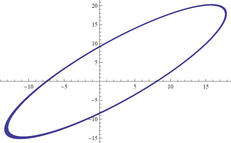
Figure 2: Regular orbit of Poincaré map ($5\cdot 10^{5}$ points)

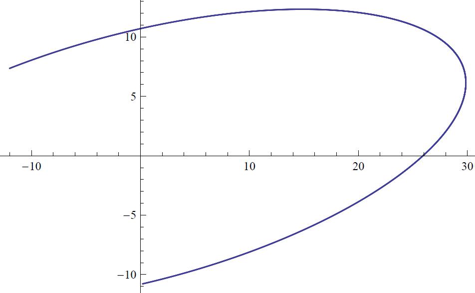
Figure 3: Regular orbit of Poincaré map ($5\cdot 10^{5}$ points)

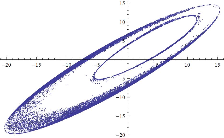
Figure 4: Chaotic orbit of Poincaré map ($5\cdot 10^{6}$ points)

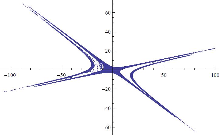
Figure 5: Chaotic orbit of Poincaré map ($5\cdot 10^{5}$ points)

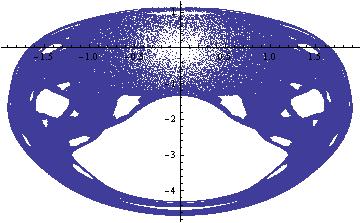
Figure 6: Chaotic orbit of Poincaré map ($5\cdot 10^{5}$ points)

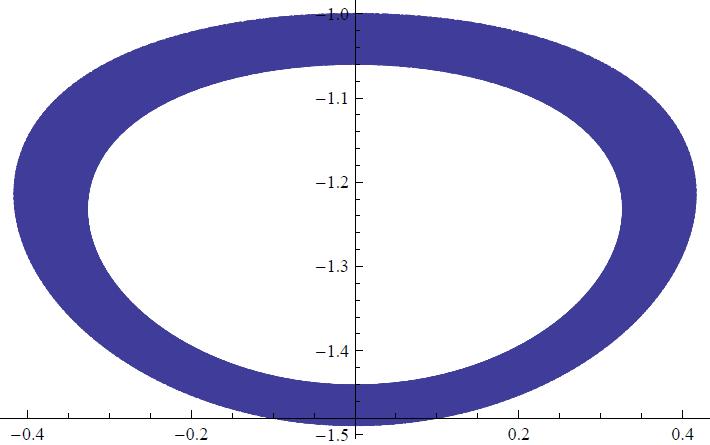
Figure 7: Chaotic orbit of Poincaré map ($5\cdot 10^{5}$ points)

5.4 Lower-dimensional projections

For special initial values of $\lambda\in L^{*}$, projections of normal geodesics $q(t)$ of the $(2,3,5,8)$-problem to certain subspaces of the state space ${\mathbb{R}}^{8}$ yield geodesics of lower-dimensional sub-Riemannian problems since there is an obvious nested chain of nilpotent SR problems on Carnot groups, like Russian Matryoshka:

$$(2)\subset(2,3)\subset(2,3,5)\subset(2,3,5,8),$$

corresponding to the chain of subspaces:

$${\mathbb{R}}^{2}_{x_{1}x_{2}}\subset{\mathbb{R}}^{3}_{x_{1}x_{2}x_{3}}\subset{\mathbb{R}}^{5}_{x_{1}\dots x_{5}}\subset{\mathbb{R}}^{8}_{x_{1}\dots x_{8}}.$$

Multiplication table in the Heisenberg algebra (growth vector $(2,3)$) is

$$[X_{1},X_{2}]=X_{3},$$ (83)

and in the Cartan algebra (growth vector $(2,3,5)$) is

$$[X_{1},X_{2}]=X_{3},\quad[X_{1},X_{3}]=X_{4},\quad[X_{2},X_{3}]=X_{5}.$$ (84)

Multiplication tables $(\ref{23})$ and $(\ref{235})$ are depicted resp. in Figs. 8 and 9 (compare with Fig. 1 for the (2,3,5,8) Carnot algebra).

Figure 8: The Heisenberg algebra

Figure 9: The Cartan algebra

If $h_{3}(\lambda)=\dots=h_{8}(\lambda)=0$, then $(x_{1}(t),x_{2}(t))$ is a Riemannian geodesic in the Euclidean plane ${\mathbb{R}}^{2}_{x_{1}x_{2}}$, i.e., a straight line.

If $h_{4}(\lambda)=\dots=h_{8}(\lambda)=0$, then $(x_{1}(t),x_{2}(t),x_{3}(t))$ is a sub-Riemannian geodesic in the Heisenberg group ${\mathbb{R}}^{3}_{x_{1}x_{2}x_{3}}$, thus the curve $(x_{1}(t),x_{2}(t))$ is a straight line or a circle [30, 6].

If $h_{6}(\lambda)=h_{7}(\lambda)=h_{8}(\lambda)=0$, then $(x_{1}(t),\dots,x_{5}(t))$ is a sub-Riemannian geodesic in the Carnot group ${\mathbb{R}}^{5}_{x_{1}\dots x_{5}}$, thus the curve $(x_{1}(t),x_{2}(t))$ is an Euler elastica — a stationary configuration of elastic rod in the plane [11, 17, 21, 22, 23, 24, 25, 26, 27], see the plots of elasticae for various values of elastic energy at Figs. 11–13.

Figure 10: Inflexional elastica

Figure 11: Inflexional elastica

Figure 12: Inflexional elastica

Figure 13: Non-inflexional elastica

For generic $\lambda\in L^{*}$, the curves $(x_{1}(t),x_{2}(t))$ look like “elasticae of variable elastic energy”, see Figs. 14, 15.

Figure 14: Elastica of variable elastic energy

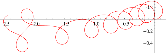
Figure 15: Elastica of variable elastic energy

There is an obvious relation of optimality of trajectories of the (2,3,5,8)-problem and its lower-dimensional projections due to the following simple statement.

Proposition 2 ([3]).

Consider two optimal control problems:

$$\dot{q}^{i}=f^{i}(q^{i},u),\quad q^{i}\in M^{i},\quad u\in U,$$

$$q^{i}(0)=q^{i}_{0},\quad q^{i}(t_{1})=q^{i}_{1},$$

$$J=\int^{t_{1}}_{0}\varphi(u)\,dt\rightarrow\min,$$

$$i=1,2.$$

Suppose that there exists a smooth map $G:M^{1}\rightarrow M^{2}$, s. t. if $q^{1}(t)$ is the trajectory of the first system corresponding to a control $u(t)$, then $q^{2}(t)=G(q^{1}(t))$ is the trajectory of the second system with the same control.

Further assume that $q^{1}(t)$ and $q^{2}(t)$ are such trajectories. If $q^{2}(t)$ is locally (globally) optimal for the second problem, then $q^{1}(t)$ is locally (globally) optimal for the first problem.

This proposition provides lower bounds for the cut time

$$t_{\operatorname{cut}}(\lambda)=\sup\{t>0\mid\pi\circ e^{s\vec{H}}(\lambda)\text{ is globally optimal for }s\in[0,t]\}$$

and the first conjugate time

$$t^{1}_{\operatorname{conj}}(\lambda)=\sup\left\{t>0\mid\pi\circ e^{s\vec{H}}(\lambda)\text{ is locally optimal for }s\in[0,t]\right\}$$

of the (2,3,5,8)-problem in terms of the same functions for its lower-dimensional projections.

For the Riemannian problem on the plane, the straight lines are optimal forever, so the cut and first conjugate times are $+\infty$, thus for the (2,3,5,8)-problem

$$h_{3}(\lambda)=\dots h_{8}(\lambda)=0\quad\Rightarrow\quad t_{\operatorname{cut}}(\lambda)=t^{1}_{\operatorname{conj}}(\lambda)=+\infty.$$

For the sub-Riemannian problem on the Heisenberg group, the circles are locally and globally optimal up to the first loop, thus for the (2,3,5,8)-problem

$$h_{3}(\lambda)\neq 0,\quad h_{4}(\lambda)=\dots=h_{8}(\lambda)=0\quad\Rightarrow\quad t^{1}_{\operatorname{conj}}(\lambda)\geq t_{\operatorname{cut}}(\lambda)\geq\frac{2\pi}{|h_{3}(\lambda)|}.$$

Similar, but much more complicated bounds hold for the case $h_{6}(\lambda)=h_{7}(\lambda)=h_{8}(\lambda)=0$ via comparison with the cut and first conjugate times for the sub-Riemannian problem on the Cartan group [21, 22, 23, 24].

6 Conclusion

We see the following interesting questions for the (2,3,5,8)-problem:

1. study optimality of abnormal geodesics,

2. describe all cases where the normal Hamiltonian vector field $\vec{H}$ is Liouville intergable, integrate and study the corresponding normal geodesics,

3. describe precisely the chaotic dynamics of the normal Hamiltonian vector field $\vec{H}$.

We plan to address these questions in forthcoming works.

References

- [1] A.A. Agrachev, Yu. L. Sachkov, Geometric control theory, Fizmatlit, Moscow 2004; English transl. Control Theory from the Geometric Viewpoint, Springer-Verlag, Berlin 2004.
- [2] A. A. Agrachev, A. A. Sarychev, Filtration of a Lie algebra of vector fields and nilpotent approximation of control systems, Dokl. Akad. Nauk SSSR, 295 (1987), English transl. in Soviet Math. Dokl., 36 (1988), 104–108.
- [3] A.Ardentov, Yu. Sachkov, Conjugate points in nilpotent sub-Riemannian problem on the Engel group, Journal of Mathematical Sciences, Vol. 195, No. 3, December, 2013, 369–390.
- [4] V.I. Arnold, Mathematical Methods of Classical Mechanics, Springer, 1997.
- [5] A. Bellaïche, The tangent space in sub-Riemannian geometry, in: Sub-Riemannian geometry, vol. 144 of Progr. Math., Birkhäuser, Basel, 1996, pp. 1–78.
- [6] R. Brockett, Control theory and singular Riemannian geometry, In: New Directions in Applied Mathematics, (P. Hilton and G. Young eds.), Springer-Verlag, New York, 11–27.
- [7] R. Montgomery, A Tour of Subriemannian Geometries, Their Geodesics and Applications. American Mathematical Society (2002).
- [8] R.Monti, The regularity problem for sub-Riemannian geodesics, Geometric Control Theory and sub-Riemannian Geometry, Springer, INdAM Series 5 (2013), G. Stefani, U. Boscain, J.-P. Gauthier, A. Sarychev, M. Sigalotti (eds.).
- [9] L.S. Pontryagin, V.G. Boltyanskii, R.V. Gamkrelidze, E.F. Mishchenko, The mathematical theory of optimal processes, Wiley Interscience, 1962.
- [10] Ch. Reutenauer, Free Lie algebras, London Mathematical Society Monographs. New Series, 7, The Clarendon Press Oxford University Press, 1993.
- [11] L.Euler, Methodus inveniendi lineas curvas maximi minimive proprietate gaudentes, sive Solutio problematis isoperimitrici latissimo sensu accepti, Lausanne, Geneva, 1744.
- [12] M. Grayson, R. Grossman, Nilpotent Lie algebras and vector fields, Symbolic Computation: Applications to Scientific Computing, R.Grossman, Ed., SIAM, Philadelphia, 1989, pp. 77–96.
- [13] M. Gromov, Carnot-Carathéodory spaces seen from within, in: Sub-Riemannian geometry, vol. 144 of Progr. Math., Birkhäuser, Basel, 1996, pp. 79–-323.
- [14] M. Hall, A basis for free Lie rings and higher commutators in free groups, Proc. Amer. Math. Soc., 1 (1950), 575–-581.
- [15] H. Hermes, Nilpotent approximations of control systems and distributions, SIAM J. Control Optim., 24 (1986), 731–-736.
- [16] A. A. Kirillov, Lectures on the orbit method, Graduate Studies in Mathematics 64, Providence, RI: American Mathematical Society, (2004).
- [17] A.E.H.Love, A Treatise on the Mathematical Theory of Elasticity, 4th ed., New York: Dover, 1927.
- [18] J. Marsden, T. Ratiu, Introduction to Mechanics and Symmetry, Springer, 1999.
- [19] A. S. Mishchenko, A. T. Fomenko, Generalized Liouville method of integration of Hamiltonian systems, Functional Analysis and Its Applications, 12 (1978), No. 2, pp 113–121.
- [20] J. Mitchell, On Carnot-Carathéodory metrics, J. Differential Geom., 21 (1985), pp. 35–-45.
- [21] Yu. L. Sachkov, Exponential mapping in generalized Dido’s problem, Mat. Sbornik, 194 (2003), 9: 63–90 (in Russian). English translation in: Sbornik: Mathematics, 194 (2003).
- [22] Yu. L. Sachkov, Discrete symmetries in the generalized Dido problem (in Russian), Matem. Sbornik, 197 (2006), 2: 95–116. English translation in: Sbornik: Mathematics, 197 (2006), 2: 235–257.
- [23] Yu. L. Sachkov, The Maxwell set in the generalized Dido problem (in Russian), Matem. Sbornik, 197 (2006), 4: 123–150. English translation in: Sbornik: Mathematics, 197 (2006), 4: 595–621.
- [24] Yu. L. Sachkov, Complete description of the Maxwell strata in the generalized Dido problem (in Russian), Matem. Sbornik, 197 (2006), 6: 111–160. English translation in: Sbornik: Mathematics, 197 (2006), 6: 901–950.
- [25] Yu. L. Sachkov, Maxwell strata in the Euler elastic problem. J. Dynam. Control Systems 14 (2008), No. 2, 169–234.
- [26] Yu.Sachkov, Conjugate points in Euler’s elastic problem, Journal of Dynamical and Control Systems, 2008 Vol. 14 (2008), No. 3 (July), 409–439.
- [27] Yu.Sachkov, E. F. Sachkova, Exponential mapping in Euler’s elastic problem, Journal of Dynamical and Control Systems, Vol. 21 (2014), in print.
- [28] Yu.Sachkov, E. F. Sachkova, Abnormal extremals in the sub-Riemannian problem, submitted.
- [29] H.Sussmann, W.Liu, Shortest parts for sub-Riemannian metrics on rank-2 distributions, Memoirs of the American Mathematical Society, No. 564, Vol. 118, November 1995.
- [30] A.M. Vershik, V.Y. Gershkovich, Nonholonomic Dynamical Systems. Geometry of distributions and variational problems. (Russian) In: Itogi Nauki i Tekhniki: Sovremennye Problemy Matematiki, Fundamental’nyje Napravleniya, Vol. 16, VINITI, Moscow, 1987, 5–85. (English translation in: Encyclopedia of Math. Sci. 16, Dynamical Systems 7, Springer Verlag.)