Trophic coherence determines food-web stability
Supporting Information
1 Food-web models
We describe here the main structural (also called static) models found in the literature for generating networks with some of the statistical features of food webs. We then discuss some aspects of the Preferential Preying Model (PPM) which we put forward in the main text (described in Methods). In all these models, the number of links can only be set in expected value. As is often done, throughout this work we discard all generated networks which have a number of links greater or smaller than this target by more than five percent. In Section 3 we describe several network measures and compare the performance of the models using the food-web data listed in Section 2.
1.1 The Cascade Model
In the Cascade Model, each species is assigned a random number drawn from a uniform distribution between and [1]. For any pair (, ), we set to be a consumer of with a constant probability if , and with probability zero if . With species, we obtain an expected number of links if we set
This was the first attempt to show how networks with a structure in some senses similar to real food webs could come about via simple rules.
Stouffer and co-workers later modified this model so that the number of prey would be drawn from the Beta distribution used by the Niche Model (see below), and called the new version the Generalized Cascade Model [2]. Since this amendment improves the model’s predictions as regards distributions of prey and predators (without, to the best of our knowledge, involving any drawbacks), throughout this paper we use the Generalized Cascade Model.
1.2 The Niche Model
In the Niche Model, each species is awarded a niche value as in the Cascade Model [3]. However, instead of choosing species with lower niche values randomly for prey, is constrained to consume the subset of species such that – i.e., all those lying on an interval of the niche axis of size and centred at , and none without. The range is defined as , where is drawn from a Beta distribution with parameters . For species and a desired number of links , we must set
The centre of the interval is drawn from a uniform distribution between and .
The rationale behind this model was that food webs were thought to be interval – i.e., the species could be arranged in an ordering such that the prey of any given predator were contiguous [4]. The Niche Model achieves this by construction. More recent analysis has shown that food webs are not generally perfectly interval, although they do usually exhibit a certain degree of intervality [5, 6]. Nevertheless, the Niche Model has been tremendously successful, since it outperforms the Cascade Model in approximating measurable features of food webs, and even compares well to more elaborate models which take the Niche Model as a basis [7]. It is still the model most commonly used whenever synthetic networks similar to food webs are required.
1.3 The Nested Hierarchy Model
The Nested Hierarchy Model provides a way to take into account that phylogenetically similar species should have prey in
common [8].
It gives each species a niche value and a range, exactly as in the Niche Model. However, instead of establishing links directly to
species within the range, first the number of prey to be consumed by each species is determined, in proportion to the range,
, so as to generate an expected number of links .
These links are then attributed in the following way.
The species with lowest niche value has no prey, while the one with the highest has no predators (so there is always at least
one basal species and one apex predator). Starting from the species with second smallest niche value and going up in order
of , we take each species and apply the following rules to determine its prey:
1. We choose a random species already in the network (so ) and set it as the first prey species of .
2. If has no predators other than , we repeat 1 until either the chosen prey does have other predators, or we
reach . Else we go to 3.
3. We determine the set of species which are prey to the predators of . We select, randomly, species from this set to
become also prey of until we either complete , or we go to 4.
4. We continue choosing prey species randomly from among those with lower niche values. If we still have not reached when
these run out, we continue choosing them randomly from those with higher niche values.
In this model, two consumers that share prey are assumed to be phylogenetically related, while the extra links that must at times be sought mimic the effects of independent adaptation. We find it a particularly interesting model because phylogenetic constraints should indeed be taken into account, and as it stands our Preferential Preying Model (described below) does not do this. One problem we find with the Nested Hierarchy Model, however, is that a given species is assumed to be related to a certain set of species which share common prey with ; but will also belong to the set of common prey of a different set of consumers, and nothing constrains and to overlap. In other words, the species related to due to its prey are not the ones related to due to its predators, whereas in nature it is to be expected that phylogenetically similar species should have both prey and predators in common. In fact, it has recently been reported that common predators are statistically more significant than common prey [9].
1.4 The Generalized Niche Model
The Generalized Niche Model was proposed to account for the fact that empirical food webs turned out not to be maximally interval, as predicted by the Niche Model [5]. A contiguity parameter was introduced, which would determine the proportion of prey to be allocated according to the Niche Model, the rest ensuing from the Generalized Cascade Model. In other words, the Niche Model would be implemented as before but with reduced ranges . Then, for each species, the number of extra prey is drawn randomly from among the available species with niche values lower than , as in the Generalized Cascade Model. For we have the Niche Model, while results in the Generalized Cascade Model.
1.5 The Minimum Potential Niche Model
The Minimum Potential Niche Model is similar to the Generalized Niche Model in that it is a modification of the Niche Model which breaks up complete intervality by means of a parameter, [12]. However, the motivation is slightly different. The idea is that in reality there is more than one niche dimension constraining possible predation links (hence the lack of complete, one-dimensional intervality), which implies that some of the links determined by the Niche Model are actually “forbidden links”. The species are all allocated niche values and ranges as in the Niche Model. The species at the extremes of this range are always consumed. However, the rest is considered a potential range and the parameter used in the Beta distribution from which is drawn is now
where , being the total number of potential links given the ranges, minus the species at the extremes. Once all the species have their ranges, each species within will be consumed with a probability . Therefore, results in the original Niche Model, but produces a proportion of forbidden links.
Allesina et al. suggested a framework for comparing niche-based models [12]; they computed the likelihood that the Cascade, Niche and Nested Hierarchy models have of generating the links in a set of ten real food webs, and found theirs (the Minimum Potential Niche Model) to be superior – and, in fact, the only one capable of generating all the observed links.
1.6 The Preferential Preying Model
In the main text we propose the Preferential Preying Model (PPM) in order to capture the trophic coherence of empirical food webs. The details are given in Methods, so here we confine ourselves to displaying the scheme diagrammatically in Fig. S1. We go on to list several possible amendments which could be made to this basic version of the model and which may be of use to researchers wishing to use the PPM for purposes other than our main one here – namely, to highlight the importance of trophic coherence and its relevance to food-web stability.

1.6.1 Possible amendments to the PPM
-
•
Basal species. All the niche-based models discussed allow the number of producers, , to emerge freely (although they are not, generally, particularly successful in predicting [7]). We chose here to begin with a set number of basal species, as in the Preferential Attachment Model [13]. We imagine that for most applications where synthetic networks are required it would be useful to have control over this parameter (which is itself related to trophic coherence, as we show in Section 3.2.3). However, if a freely emerging were preferred – for instance, for a rigorous comparison against models which do not allow this value to be set easily – it is straightforward to take the minimum equal to zero for incoming species, thereby allowing a proportion of them to become producers.
-
•
Numbers of prey. We have drawn the number of prey for each incoming species from a Beta distribution, as in all the niche-based models, because Stouffer et al. [2] have shown that this method yields a particularly good fit to food-web data (we have also verified that this holds true for our 46 food-web dataset). However, were the model to be applied to systems other than food webs, it may be preferable to use, for instance, a Poisson or a Pareto distribution, depending on the in-degree distributions of the networks to be emulated.
-
•
Boltzmann factor. The functional form we have used to determine the second and subsequent prey of an incoming species (an exponential in the trophic distance divided by the parameter ) is arbitrary; careful fitting to data may suggest a better function. There is also no reason other than simplicity to use the same value of for each incoming species: one could also draw a different value for each incoming species form some distribution, perhaps dependent on the trophic level of its first prey.
-
•
Cycles. Directed loops in food webs are relatively rare, yet often present. The PPM as described does not generate any of these cycles, but it could easily be amended to do so by assigning each incoming species a small number of predators as well as prey from amongst the species already in the network. However, directed loops require some predators to consume prey at higher trophic levels than theirs, so the more coherent a network, the fewer directed loops are to be expected.
-
•
Phylogeny and body size. In this simple incarnation, the PPM ignores the main effects that most of the other models are based on, but these could be taken into account in a “Generalized Preferential Preying Model”. Something akin to a phylogenetic signal could be induced by introducing a bias in the Boltzmann factor such that an incoming node tended to copy the prey and predators of a randomly chosen species already in the network – perhaps limiting in the Nested Hierarchy Model in the case where only prey are copied. The Niche, Generalized Niche and Minimum Potential Niche models assume that the niche ordering (usually thought to represent body size, possibly in combination with other biological features) to some extent constrains species to find prey within closed intervals thereof. A bias could likewise be introduced in the Boltzmann factor of the PPM such that intervals of the sequence of entry were preferred, if this constraint in empirical networks turned out to be more than a spurious effect of trophic coherence.
1.6.2 Negative temperatures
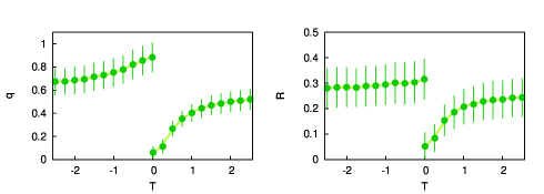
As discussed in the main text, the PPM can generate any level of trophic coherence between that of a maximally coherent structure (with ) and one as incoherent as would be obtained if attachment were random (at ). However, as shown in Table SLABEL:table_foodwebs, some food webs (five out of the 46 in our dataset) exhibit higher values of even than this latter case. The PPM can also generate greater incoherence than obtained at high positive with negative values of this parameter, as illustrated in Fig. S2. The curves of and would be continuous if instead of we used its inverse, . With this parameter, corresponds to random attachment, with falling monotonically from maximum incoherence at to maximum coherence at . A comparison of the two panels in Fig. S2 shows that the effect of trophic coherence on stability seems to saturate at about the obtained with random attachment: greater incoherence has little effect on .
2 Food-web data
We have compiled a dataset of 46 food webs available in the literature, pertaining to several ecosystem types. The methods used by the researchers to establish the links between species vary from gut content analysis to inferences about the behaviour of similar creatures. In Table SLABEL:table_foodwebs we list the food webs used along with references to the relevant work. We also list, for each case, the number of species , of basal species , the mean degree , the ecosystem type, the trophic coherence , the value of the parameter found to yield (on average) the empirical with the Preferential Preying Model, and the numerical label used to represent the food web in several figures below.
| Food web | Type | Reference | Label | |||||
| Akatore Stream | 84 | 43 | 2.70 | River | 0.16 | 0.26 | [16, 17, 18] | 18 |
| Benguela Current | 29 | 2 | 7.00 | Marine | 0.76 | 0.87 | [19] | 11 |
| Berwick Stream | 77 | 35 | 3.12 | River | 0.18 | 0.25 | [16, 17, 18] | 34 |
| Blackrock Stream | 86 | 49 | 4.36 | River | 0.19 | 0.25 | [16, 17, 18] | 27 |
| Bridge Brook Lake | 25 | 8 | 4.28 | Lake | 0.59 | 1.15 | [20] | 14 |
| Broad Stream | 94 | 53 | 6.01 | River | 0.16 | 0.16 | [16, 17, 18] | 35 |
| Canton Creek | 102 | 54 | 6.83 | River | 0.16 | 0.18 | [21] | 2 |
| Caribbean (2005) | 249 | 5 | 13.31 | Marine | 0.75 | 0.70 | [22] | 17 |
| Caribbean Reef | 50 | 3 | 11.12 | Marine | 0.99 | -0.24 | [23] | 13 |
| Carpinteria Salt Marsh Reserve | 126 | 50 | 4.29 | Marine | 0.65 | -8.27 | [24] | 33 |
| Catlins Stream | 48 | 14 | 2.29 | River | 0.20 | 0.27 | [16, 17, 18] | 19 |
| Chesapeake Bay | 31 | 5 | 2.19 | Marine | 0.47 | 0.67 | [14, 15] | 5 |
| Coachella Valley | 29 | 3 | 9.03 | Terrestrial | 1.34 | -0.02 | [25] | 12 |
| Crystal Lake (Delta) | 19 | 3 | 1.74 | Lake | 0.28 | 0.33 | [26] | 37 |
| Cypress (Wet Season) | 64 | 12 | 6.86 | Terrestrial | 0.63 | 0.73 | [27] | 42 |
| Dempsters Stream (Autumn) | 83 | 46 | 5.00 | River | 0.23 | 0.30 | [16, 17, 18] | 36 |
| El Verde Rainforest | 155 | 28 | 9.74 | Terrestrial | 1.02 | -0.82 | [28] | 15 |
| Everglades Graminoid Marshes | 63 | 5 | 9.79 | Terrestrial | 0.66 | 0.47 | [29] | 44 |
| Florida Bay | 121 | 14 | 14.60 | Marine | 0.59 | 0.48 | [27] | 26 |
| German Stream | 84 | 48 | 4.20 | River | 0.21 | 0.29 | [16, 17, 18] | 28 |
| Grassland (U.K) | 61 | 8 | 1.59 | River | 0.40 | 0.72 | [30] | 4 |
| Healy Stream | 96 | 47 | 6.60 | River | 0.22 | 0.24 | [16, 17, 18] | 29 |
| Kyeburn Stream | 98 | 58 | 6.42 | River | 0.18 | 0.18 | [16, 17, 18] | 30 |
| LilKyeburn Stream | 78 | 42 | 4.81 | River | 0.23 | 0.29 | [16, 17, 18] | 31 |
| Little Rock Lake | 92 | 12 | 10.84 | Lake | 0.69 | 0.75 | [31] | 8 |
| Lough Hyne | 349 | 49 | 14.66 | Lake | 0.62 | 0.66 | [32, 33] | 46 |
| Mangrove Estuary (Wet Season) | 90 | 6 | 12.79 | Marine | 0.67 | 0.47 | [27] | 43 |
| Martins Stream | 105 | 48 | 3.27 | River | 0.32 | 0.49 | [16, 17, 18] | 20 |
| Maspalomas pond | 18 | 8 | 1.33 | Lake | 0.48 | -9.22 | [34] | 39 |
| Michigan Lake | 33 | 5 | 3.91 | Lake | 0.38 | 0.21 | [35] | 40 |
| Mondego Estuary | 42 | 12 | 6.64 | Marine | 0.74 | 10.07 | [36] | 41 |
| Narragansett Bay | 31 | 5 | 3.65 | Marine | 0.66 | 1.18 | [37] | 38 |
| Narrowdale Stream | 71 | 28 | 2.18 | River | 0.25 | 0.38 | [16, 17, 18] | 21 |
| N.E. Shelf | 79 | 2 | 17.76 | Marine | 0.82 | 0.67 | [38] | 10 |
| North Col Stream | 78 | 25 | 3.09 | River | 0.28 | 0.34 | [16, 17, 18] | 22 |
| Powder Stream | 78 | 32 | 3.44 | River | 0.22 | 0.28 | [16, 17, 18] | 23 |
| Scotch Broom | 85 | 1 | 2.62 | Terrestrial | 0.45 | 0.49 | [39] | 16 |
| Skipwith Pond | 25 | 1 | 7.88 | Lake | 0.68 | 0.23 | [40] | 6 |
| St. Marks Estuary | 48 | 6 | 4.60 | Marine | 0.69 | 1.02 | [41] | 9 |
| St. Martin Island | 42 | 6 | 4.88 | Terrestrial | 0.59 | 0.60 | [42] | 7 |
| Stony Stream | 109 | 61 | 7.61 | River | 0.17 | 0.18 | [43] | 3 |
| Sutton Stream (Autum) | 80 | 49 | 4.19 | River | 0.15 | 0.19 | [16, 17, 18] | 32 |
| Troy Stream | 77 | 40 | 2.35 | River | 0.18 | 0.30 | [16, 17, 18] | 24 |
| Venlaw Stream | 66 | 30 | 2.83 | River | 0.23 | 0.33 | [16, 17, 18] | 25 |
| Weddell Sea | 483 | 61 | 31.81 | Marine | 0.75 | 1.01 | [44] | 45 |
| Ythan Estuary | 82 | 5 | 4.82 | Marine | 0.46 | 0.38 | [45] | 1 |
3 Network measures
3.1 Trophic coherence
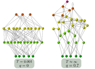
In the Methods section of the main text we define the network structural property of trophic coherence. Here we simply illustrate the difference between a maximally coherent network and a highly incoherent one in Fig. S3.
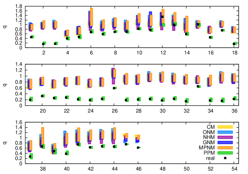
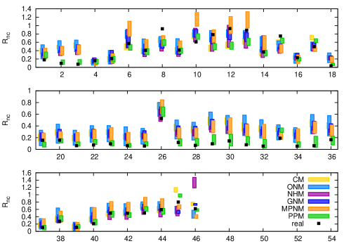
In Fig. S4 we show the empirical values of observed in each of the 46 food webs (also displayed in Table SLABEL:table_foodwebs) along with the predictions of each of the food-web models discussed above and in the main text.
3.2 Stability
Let us assume that we have a set of ordinary differential equations governing the evolution of the population of each species in an ecosystem, as measured, for instance, by its total biomass . In vector form, we can write this as
The dynamics will have a fixed point at any configuration such that . Let us suppose that the system is placed at this fixed point but suffers a small perturbation :
For small enough , its dynamics will be given by the linearised equation:
where is the Jacobian matrix evaluated at . The fixed point will be locally stable if all the eigenvalues of have negative real part [46].
Let us consider a fairly general dynamics for given by a consumer-resource model:
| (1) |
The first term on the right accounts for the increment in species ’s biomass through consumption of its resources, the second term is the biomass lost to its consumers, and the function represents any factors which are not due to interaction with other species. Since we are interested here in effects of interactions between species, we shall simply assume with a constant. The function describes how the interaction between a consumer and a resource species depends on their respective biomasses. The parameter is the efficiency of predation – the proportion of biomass lost by a resource which goes on to form part of the consumer. We shall in general consider this parameter to be constant for all pairs of species (, ), but in Sections S3.2.2 and S3.2.4 we look into the effects of varying its value. In the main text, we set this parameter to .
The Jacobian, , will be obtained by taking the partial derivatives of Eq. (1), for each , with respect to each .
In the simple case where the interaction between species is given by a sum,
we have
where is the Kronecker delta (equal to one when , or else zero). Positive terms added to or subtracted from the main diagonal of simply shift its spectrum of eigenvalues to the right or left, respectively. Therefore, we concentrate on the matrix
| (2) |
where is the transpose of , and consider , the eigenvalue of with the largest real part. Then, can be regarded as a measure of the minimum degree of self-regulation at each node which this dynamics would require in order for the system to be stable. In other words, the smaller , the more stable we shall say the system is.
In this simple case defined by the Jacobian is independent of the point where it is evaluated. However, this will not, in general, be the case and for other dynamics we would need to specify this point in order to characterise the stability of the system. For instance, in a generalised Lotka-Volterra dynamics, the interaction is proportional to the biomass of both consumer and resource,
and the Jacobian becomes
| (3) |
where are the elements of the matrix as given by Eq. (2). Note that this expression depends on the biomass of species (though not on ’s) at the point of interest.
To capture the nonlinearities expected in a prey species’ functional response, consumer-resource models often describe the interaction as
where is the Hill equation,
with the half-saturation density. The Hill coefficient determines whether the functional response is of type II () or type III () [47]. Now we find that the Jacobian is
| (4) |
if , where the effective efficiency of predation is
and, for the main diagonal elements,
In each of these kinds of dynamics it is necessary to evaluate the Jacobian at a particular point: Equations (3) (Lotka-Volterra) and (4) (types II and III) are similar in form to the matrix of Eq. (2), but their terms are modified by the biomass of the predator, or the biomasses of both prey and predator, respectively. One might suggest that we only need identify a fixed point and evaluate the equations there. But, in general, a feasible fixed point (in which for all ) will not exist. Feasible fixed points could be defined by attributing weights to the elements of the interaction matrix , but this would involve decisions on how to do this in a realistic way which might render the results somewhat arbitrary. (For a discussion on the feasibility of fixed points, see Section S3.2.5.)
Throughout most of the paper we focus simply on the matrix as given by Eq. (2), for although the dynamics it describes exactly is not very realistic (corresponding to the interaction term in Eq. (1)), it captures the essential behaviour of better motivated dynamics without requiring any assumptions about the fixed point. In fact, if all species had the same biomass at the fixed-point, then Eqs. (3) (Lotka-Volterra) and (4) (types II and III) would also reduce to the matrix as given by Eq. (2), for an appropriate choice of the parameter . However, so as to test the robustness of our results to details of the dynamics, in Section S3.2.1 we look into the effects of different distributions of biomass according together with Lotka-Volterra, type II or type III dynamics. We find that the relationship between trophic coherence and stability reported in the main text is robust to these considerations, although the dependence of biomass on trophic level introduces interesting effects, in particular for the complexity-stability scaling.
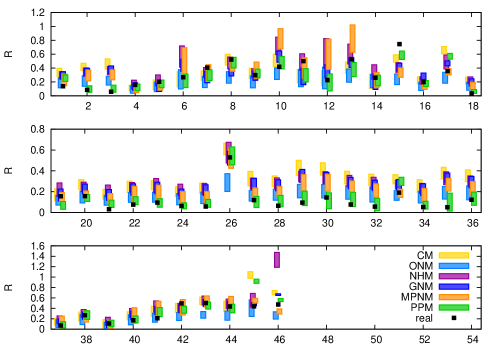
In the main text we describe how stability in directed networks (and food webs in particular) is determined to a large extent by their trophic coherence. In Fig. S5 we compare the predictions of each of the food-web models described in Section 1 for each of the food webs listed in Table LABEL:table_foodwebs. Another network feature which influences stability, as mentioned above, is the existence of self-links (representing cannibalism, in the case of food webs), since this is a form of self-regulation. We disentangle this effect from that of trophic coherence, we remove all self-links from the food webs and again measure the real part of the leading eigenvalue, . The predictions of each model are shown in Fig. S6.
In Section 4 we give a proof that a maximally coherent network () with constant interaction strengths can always be stabilised with an infinitesimal degree of self-regulation.
3.2.1 Biomass distribution
As discussed in Section S3.2, the Jacobian corresponding to most kinds of biologically plausible dynamics will depend on details of the fixed point. In other words, we need to know the biomass of each species in order to evaluate the Jacobian. Since only a fraction of the energy produced by a species can be used by its consumers, ecosystems can often be regarded as pyramids in which biomass is a decreasing function of trophic level [48]. More specifically, if we assume that the biomass of a species is a constant fraction of the combined biomass of its resources, biomass will be exponentially related to trophic level. We can thus write
| (5) |
with a parameter determining the difference in biomass between predator and prey species (for there is no dependence of biomass on trophic level), and set the basal species to unity biomass. A negative value of then corresponds to a pyramid in which biomass decreases with trophic level (note that a graphical representation of this situation will look like a pyramid if the size of each echelon corresponds to the logarithm of its biomass). Although terrestrial food webs have this distribution, in certain aquatic environments inverted pyramids can arise, corresponding to a positive . This is due to the effect of increasing longevity with trophic level, which can compensate to some extent for the inefficiency of predation [48].
In order to examine the robustness of results to fluctuations in this exponential law, we can consider instead a biomass given by
| (6) |
where the variables are randomly drawn from a normal distribution with mean zero and standard deviation . We can then use these values of to evaluate the Jacobian for each kind of dynamics and study the behaviour of its leading eigenvalue, .
| Jacobian | (no self-links) | |||
Table SLABEL:table_TYPE shows the correlations between stability and the various network measures shown in Fig. 1 of the main text over the 46 food webs in the dataset. The first row displays the values for the simple case where the Jacobian is considered equal to the interaction matrix . The second, third and fourth rows are for the cases of Lotka-Volterra, type II and type III dynamics, with biomass distributed according to Eq. (5) and . The general pattern shown in Fig. 1 of the main text is conserved for these more realistic dynamics.
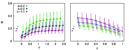
In Fig. 7 we show the values of obtained from the Lotka-Volterra Jacobian given by Eq. (5) with different values of , corresponding to pyramid, flat and inverted pyramid distributions of biomass. The empirical values found for the Chesapeake Bay food web [14, 15] with each distribution are compared to the predictions of the Preferential Preying Model against (left panel), and the Generalized Niche Model against contiguity (right panel). The effect of the parameter on stability in the PPM networks remains qualitatively the same as the results reported in the main text for the matrix given by Eq. (2). The more squat the biomass pyramid (the more negative the parameter ), the more stable are both the empirical and PPM networks. This is in keeping with observations of ecosystems [48]. In the Generalized Niche Model networks, however, the effect is opposite: it is the inverted pyramid (positive ), which is most stable. We do not have an explanation for such an effect, but note that it marks a qualitative difference between the networks generated with this model and real food webs.
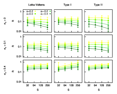
In Fig. 8 we look into how the biomass distribution affects the diversity-stability relationship. All networks are generated with the Preferential Preying Model and . The first row of panels is for the case where biomass decays with trophic level as an uncorrupted exponential (), for Lotka-Volterra, type II and type III dynamics (top panels from left to right). As compared with the constant biomass case (), a decaying distribution is seen to increase the slope whereby falls with . In other words, placing more biomass at the bottom of the food web than at the top not only increases stability, but also strengthens the positive diversity-stability relationship exhibited by trophically coherent networks. This occurs for all three kinds of dynamics, although the effect is strongest for type III and weakest for type II. For an inverted pyramid (positive ), is approximately constant with .
We go on to analyse the effect of corrupting the exponential distribution of biomass with a noise of standard deviation . The second row of panels is for . Although the slope is now less pronounced in all cases, this degree of noise does not undermine the positive diversity-stability relationship for any of the dynamics considered. Finally, in the bottom row we apply a higher noise, . Now the relationship is inverted and diversity decreases stability. It is not, perhaps, surprising that noise in the distribution of biomass (large ) should have a similar effect on scaling as incoherence in the trophic structure (large ). However, it is interesting that the noise level at which the transition from a positive to a negative diversity-stability relationship occurs does not seem to depend on or on the kind of dynamics.
3.2.2 Efficiency
According to the definition of above, we must give a value to the parameter in order to measure stability. The value of this parameter affects the kind of interaction we intend to model with the interaction matrix, , and has a strong bearing on the values of measured. The definition of captures the fact that the effect of a prey species on one of its predators is a proportion of the effect of the predator on the prey. If we are considering the flow of biomass from prey to predator, this should be a relatively small fraction – for instance, the “ten percent law” is often used as a rough estimate of the efficiency of predation [49]. On the other hand, our definition of stability is only strictly independent of the fixed point for a dynamics such as the one described above. For a more realistic dynamics, we might expect a multiplicative factor to appear relating the fixed-point biomass of a prey species to that of one of its predators. The parameter might therefore be increased (or decreased) by this effect.
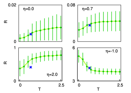
As mentioned above, throughout the paper we use the value . However, simulations of the PPM show that using the value of the parameter which best approximates the empirical degree of trophic coherence is enough to predict the empirical for a wide range of . In Fig. S9 we show against for PPM networks constructed with the parameters of the Chesapeake Bay food web [14, 15] for four cases. We also plot, with an asterisk, the empirical value of observed in each case, always at the value found to adjust the empirical trophic coherence, (see Table SLABEL:table_foodwebs). The top left panel is for the case of , which represents a situation in which the biomass of prey species is completely unaffected by the biomass of their predators. We show in the proof we include in Methods that a perfectly coherent network with would have only zero eigenvalues. As incoherence increases, grows somewhat, though it remains small compared to most cases in which the parameter simulates a measure of feedback from predators to prey. The top right panel is for , implying a relatively high efficiency and a strong negative feedback acting on prey species. At , all the eigenvalues of would have zero real part because it would be an antisymmetric matrix (intuitively, any increase in one node’s biomass will be compensated by a decrease in another, so perturbations will be maintained and neither dampened nor amplified). At we simulate a situation such that a predator extracts more biomass form its prey than the latter loses. As we would expect intuitively, this scenario of runaway growth is significantly more unstable than the ones described above. However, the behaviour of with is qualitatively similar to that observed for . Finally, the bottom right panel corresponds to the case , implying that predation reduces the biomass of a predator as well as that of its prey. We know from the proof described in Methods that at all the eigenvalues of are purely real for any . Similarly, the behaviour of with is now inverted: the most coherent networks are now the most unstable.
In the panels corresponding to , and , the value of which adjusts the empirical trophic coherence also predicts the empirical very accurately (as we have found for all the food webs in our dataset when using ; see main text). The case of is slightly out: the PPM predicts a slightly higher value of at , although it is not out by much more than a standard deviation. This case of is unlikely to be relevant for ecology; but the small discrepancy serves to remind us that the PPM does not capture all the structural features of real food webs.
3.2.3 Herbivory
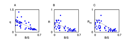
Links from basal species (producers) to species which only consume basal species (herbivores) will necessarily have a trophic distance equal to one (see Methods in the main text). Since the proportion of basal species, , varies considerably among food webs, we can expect this measure to have a strong bearing on trophic coherence. On the other hand, a large number of basal species may provide a more stable configuration than a network in which many species depend on just a few producers. Might this be the underlying reason for the relation between trophic coherence and stability?
Figure S10A is a scatter plot of against for the food webs listed in Table SLABEL:table_foodwebs. There is indeed a significant negative correlation (). Figures S10B and S10C show how stability, as measured both before and after removing self-links, varies with the proportion of basal species in the same dataset. The correlations are also significant ( for and for ), but slightly lower than we observe in Fig. S10A. In any case, they are much weaker than the correlations shown in Fig. 1 of the main text between trophic coherence and stability. We can therefore conclude that trophic coherence is the most powerful explanatory variable of stability, while the effect of the proportion of basal species is either less important, or simply an artefact of its correlation with trophic coherence.
3.2.4 Weighted networks
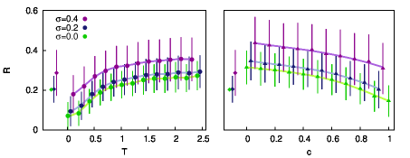
Although we have been considering the food webs as unweighted networks (the elements in are either zero or one), in reality certain interactions will be more important than others, and the efficiency need not be the same for all links. A simple way to look into how these considerations might affect our results is as follows. We make the change , with drawn from a Gaussian distribution of mean zero, standard deviation and no correlation between and . For a given network we then obtain the value of for many different realizations of the noise . In the left panel of Fig. S11 we show the average and standard deviations of thus defined for three different levels of noise – , and – for PPM networks with the parameters of the Chesapeake Bay food web [14, 15]. We also show (with diamonds) the corresponding averages and standard deviations obtained by performing the same test on the empirical food web. As is to be expected, increased noise leads to a higher average (lower stability) and a wider standard deviation. However, the behaviour of the average against the parameter remains similar with increasing noise, and the value which best adjusts the empirical trophic coherence (as given by Table SLABEL:table_foodwebs) continues to predict the empirical average at each . This is not, however, the case for the Generalized Niche Model. We show the mean and standard deviation of generated with this model against its contiguity parameter for the same food web. Whereas the empirical and simulated average values of correspond at when there is little noise, as increases the model average grows faster than the empirical value. This suggests that trophically coherent networks, such as the Chesapeake Bay food web or those generated by the PPM, are more robust to fluctuations in interaction strengths than those generated with niche-based models.
The allometric relationship according to which metabolic rates decline with increasing body size has been shown to reduce predation strength per unit biomass, thereby contributing to stability [50]. Since body size tends to augment (exponentially) with trophic level, this would mean that a more coherent structure would also involve a more homogeneous distribution of link strengths (for a given predator). Therefore, in a more realistic setting in which body sizes and link strengths are considered, we expect the stabilising effect of trophic coherence to be greater than we have shown here for binary networks.
3.2.5 Feasibility
We have been discussing the potential stability of fixed points of ecosystem dynamics, but for this to be relevant such a fixed point has to be feasible. That is, there must exist a fixed point such that every species has a positive biomass. To determine a potential fixed point one must, in general, know the details of the dynamics (as mentioned above). However, even with these specifications, given an unweighted network is is highly unlikely that the fixed point will involve only positive biomasses. However, nature does not have this problem, among other reasons because species’ biomasses co-evolve with the interaction weights. If we are granted a certain freedom to set these weights, even if other details of dynamics are set, the problem of finding a fixed point becomes under-specified, and configurations allowing for feasible fixed points might be located. We saw above that the stability of real food webs and those generated by the PPM seem to be more robust to random changes in interaction strengths than their niche-based model counterparts. This suggests that, given a prescription to modify interaction weights, trophic coherence might enhance the feasibility of fixed points as well as their stability. Such an exercise lies beyond the scope of this paper, but we believe it is a promising avenue of research to be undertaken in the future.
3.2.6 Stability criteria
In the main text we discuss May’s result for random networks, according to which the real part of the leading eigenvalue should scale as . We also show that does not exhibit a significant correlation with , although we do observe a modest positive correlation () with . In Figs. S12A and S12B we show scatter plots, for the food webs listed in Table SLABEL:table_foodwebs, of the leading eigenvalue after self-links have been removed, , against and . In the former case the correlation is now negative but still insignificant, while in the latter the correlation increases slightly to . However, food webs are network in which all the links stand for predation (as opposed to other ecological relationships, such as competition or mutualism). Allesina and Tang have recently derived stability criteria for specific kinds of interactions [51]. In particular, when the links stand for predation but are randomly placed among the species, they find that the real part of the leading eigenvalue should scale as
| (7) |
where is the variance of the off-diagonal elements of the interaction matrix , and is Pearson’s correlation coefficient between the elements and . Figure 12C is a scatter plot of against the prediction of Eq. (7). Somewhat surprisingly, the correlation is very weak (). In Fig. 12D we swap for (the leading eigenvalue when cannibalism is included) and now the correlation becomes significant (), although still relatively low. These results provide further evidence that the structure of food web is non-random in a way which is particularly relevant for their stability.

3.2.7 Missing links and trophic species
Despite important recent developments in food-web inference techniques, it is often hard to ascertain from observation whether a given species consumes another (and even more difficult to quantify the extent of predation). Furthermore, the food webs we have used here for our analysis (described in Section 2) were obtained with a variety of different techniques. To assess whether the patterns we have observed in this dataset, shown in Fig. 1 of the main text, are robust to possible experimental errors, we remove from each food web a percentage of links, chosen randomly, and recompute each of the magnitudes of interest. After averaging over 100 such tests for each food web, we then recalculate each of the correlation coefficients shown in Fig. 1. These are shown in Table SLABEL:table_deletion for different percentages of links removed. As we can see, the dependency of stability on the other magnitudes is barely affected by the random deletion of links: the correlation of with size is never significant, while the correlation with both complexity and coherence actually increases slightly with the percentage of deleted links.
| Missing links | (no self-links) | |||
The nodes in the food webs found in the literature often represent “trophic species”. This means that if two or more species in the community share their full sets of prey and predators, they are coalesced into a single node, even if they are in fact taxonomically distinct. However, with recent advances in empirical techniques of food-web inference, larger networks are now being obtained in which nodes represent taxonomic, rather than trophic, species. To find out whether our empirical findings are affected by the degree of taxonomic resolution, we perform a similar test to that of link deletion: for each food web, we randomly choose a percentage of species to be duplicated – that is, we introduce a new species with the same sets of predators and prey. As before, we average over 100 such tests and recalculate the correlation coefficient for each pair of magnitudes of interest. In Table SLABEL:table_duplicity we show these results for various percentages of duplicated species. As with the deleted links, we find that the correlations are fairly robust to these modifications, implying that they are not severely affected by the taxonomic resolution of the food webs.
| Species duplicated | (no self-links) | |||
3.3 Mean chain length
A food chain is a directed path beginning at at basal species (one with no in-coming links) and ending at an apex predator (one with no out-going links) [52]. In other words, it is any one of the possible paths that biomass entering the system through a basal species can follow until it is entirely dissipated. A food web generally has a very large number of such chains; but a low mean chain length (MCL) – an average over all of them, the length of a chain being the number of links it comprises – has been associated with a high stability [53].
All food webs representing a more or less autonomous ecosystem necessarily have at least one basal species; however, it can occur that there are in fact no apex predators. This is because the top predators can eat each other. To get round this we define an apex set as a group of predators such that no directed paths leave the group, while they would if any member of the set were removed. For instance, say predator A and predator B would both be apex in the usual sense if it weren’t because they ate each other. With this definition they form, together, an apex set. Thus, we define a food chain as a directed path beginning at a basal species and ending in any species belonging to an apex set. In this section, we shall use the term “apex predator” to refer to any member of an apex set.
To find the apex sets in a given food web, we make use of random walkers: imaginary beings that move through the network hopping from one node to another along links (in the direction allowed). The walkers are called random because at each hop they choose randomly between the different nodes they can access. Random walkers are often used to study diffusion processes, and here they can be thought of as representing the diffusion of biomass through the food web. Given a network, we simulate many such random walkers beginning at basal species, and for each node we keep a register of how many times it has been visited. When the walkers reach an apex set, they cannot leave it, and will forever continue to hop around among the members of the group (or they might stay at a single species if it is apex in the original sense, since there is nowhere to hop). Therefore, whereas most nodes will be visited a small number of times which is independent of how long we allow each walker to “live”, the number of times the apex predators are visited increases with walker longevity. This provides a simple computational way of finding the apex predators which, though stochastic, will always determine the sets exactly.
Once we know the basal and apex species, we can proceed to find all the chains and obtain the mean value of their length. At least this is possible in principle – in practice, the number is often prohibitively large to be calculated exhaustively. We therefore make use again of the random walkers. We just have to simulate many walkers beginning at basal species and remove them when they arrive at an apex predator, counting how many steps it took them to get there. There is, however, a caveat. The chains actually used provide a biased sample of all the chains in the food web: a long chain is more likely to be abandoned somewhere along its length than a short one. More precisely, the probability that a particular chain, , has of being used is inversely proportional to
the product extending over all the species in (except the apex predator), and where is the number of predators of species . So to take this bias into account we calculate, for each walker , not only the length of the path it uses, , but the value , where is the path taken by . After doing this for walkers, an estimate of the mean chain length (which will be more accurate the larger ), is
We made sure that this stochastic method converges to the right MCL by comparing the values returned with the results from exhaustive searches for those networks where this was possible.
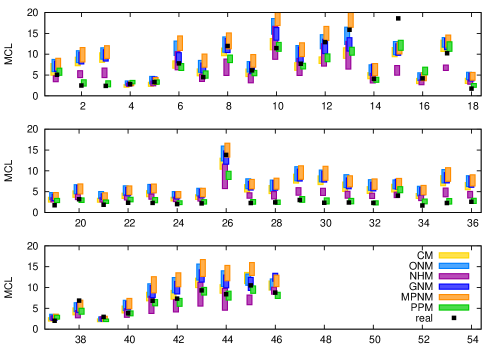
Figure S13 shows the predictions of MCL made by each food-web model for the food webs listed in Table SLABEL:table_foodwebs.
3.4 Modularity
Much attention has been paid in recent years to the community structure of complex networks: how the nodes can be classified in groups – or modules – such that a high proportion of links fall within groups. For a network with nodes and mean degree , the configuration model holds that the probability of there being a link from to is (where and are the numbers of ’s prey and predators, respectively) [54]. Using this, and given a particular partition (i.e., a classification of nodes into groups) of the network, one can define
where is a label corresponding to the partition that node finds itself in, and is the Kronecker delta [54]. The modularity of the network is taken to be the maximum value of obtainable with any partition. Since searching exhaustively is prohibitive for all but very small and sparse networks, a stochastic optimization method is usually called for. We use the algorithm of Arenas et al. [55], although there are many in the literature and the most appropriate can depend on the kind of network at hand [56].
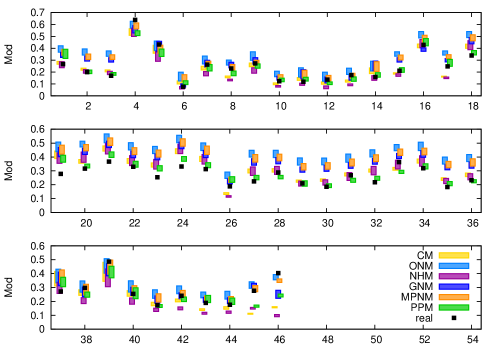
Figure S14 shows the predictions of modularity made by each food-web model for the food webs listed in Table SLABEL:table_foodwebs.
3.5 Cannibals and apex predators
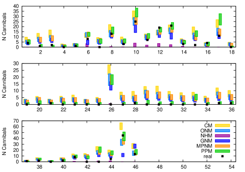
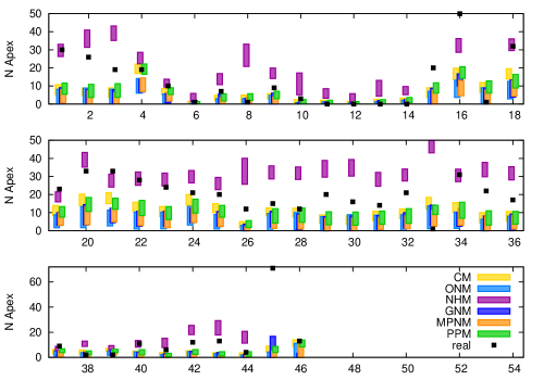
As we have discussed above, cannibalism contributes significantly to stability. We show the number of species with self-links predicted by each food-web model for the food webs listed in Table SLABEL:table_foodwebs in Fig. S15. We also measure the number of apex predators – in the conventional sense of those with no consumers – and display the model predictions in Fig. S16.
3.6 Mean trophic level
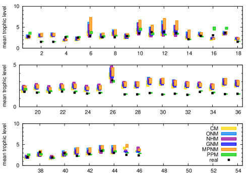
The last network feature we analyse is the mean trophic level, which is simply an average over all the species in a food web of their trophic levels (i.e., ). Thanks to Pauly and colleagues’ seminal paper “Fishing down marine food webs” [57], the mean trophic level has come to be regarded as an indicator of an ecosystem’s health, to the extent that the Convention on Biological Diversity has mandated that signatory states report changes in this measure (renamed the Mean Trophic Index) for marine ecosystems. The model predictions for the mean trophic level are displayed Fig. S17.
3.7 Comparison of network measures
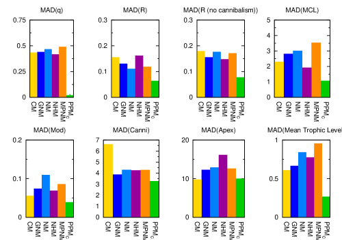
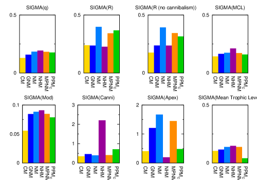
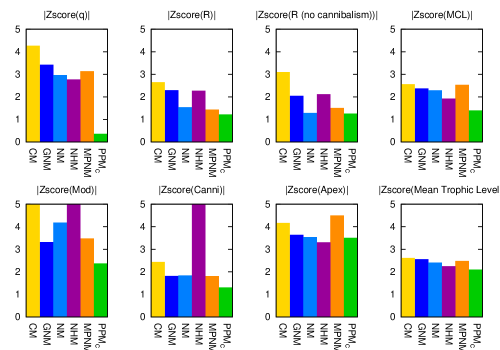
For each of the food-web models and each network measure, we can compute the Mean Average Deviation (MAD) of the theoretical prediction, from the empirical value, , simply as , where stands for an average over the 46 food web listed in Table SLABEL:table_foodwebs. The results for each of the eight network measures are shown in the panels of Fig. S18. The first panel sums up what we can observe in Fig. S4 – that the niche-based models tend to overestimate the value of significantly. The fact that none of these models differs substantially as regards from the predictions of the Cascade Model implies that the various features which they are designed to capture – such as intervality, multiple niche dimensions or phylogenetic constraints – have very little bearing on trophic coherence. The Preferential Preying Model, on the other hand, can reproduce the correct value of in 45 out of 46 food webs by adjusting its parameter . The odd web out is that of Coachella Valley, which is slightly more incoherent even than the PPM achieves with low, negative . This food web is also the only one in our dataset in which more than half the species indulge in cannibalism. As can be seen from a comparison of Figs. S5 and S6, this allows the Coachella Valley food web to exhibit a relatively low , which it loses when we remove self-links.
The second and third panels show how the models fare as regards stability, both with and without self-links. As discussed in the main text, the PPM achieves significantly better results than the other models in both cases, something we attribute to its reproducing the correct level of trophic coherence. Furthermore, in Figs. S5 and S6 we observe that the niche-based models tend to predict less stability than the food webs exhibit, especially in the case without cannibals. This is in keeping with the observation by Allesina and Tang [51] that “realistic” food web structure (i.e., that generated with current structural models) is not conducive to stability.
Next we look at mean chain length and modularity, two measures which have been associated with ecosystem robustness. In particular, a low mean chain length is thought to increase stability [53], while a high modularity might contain cascades of extinctions [10]. In keeping with the first observation, the niche-based models tend to predict longer chains than found in nature; however, they also somewhat overestimate modularity. In any case, the PPM also outperforms the other models on these two measures.
The numbers of cannibals and of apex predators are not very well predicted by any of the models. All but the Nested Hierarchy Model tend to overestimate the cannibals and underestimate the apex predators. Finally, we look at the mean trophic level – a measure which, as mentioned above, is used nowadays to assess the health of marine ecosystems and to monitor the effects of overfishing [57]. As we might expect from this measure’s relationship to trophic structure, the PPM does significantly better than the other models at predicting the mean trophic level of food webs. In general, the niche-based models tend to overestimate the mean trophic level, as shown in Fig. S17.
The standard deviations around the Mean Absolute Deviation measures of Fig. S18, relative to each mean value, are displayed in Fig. S19. In Fig. S20, we show the absolute values of the mean z-score obtained for each of the models on the same measures.
The comparison we have made here is not as rigorous as one might wish to establish the best food-web model, and this was not our intention. For instance, we have not controlled for the number of parameters, nor attempted to derive likelihoods for each model, as Allesina et al. have done [12]. There are also, of course, many other network measures of interest in ecology which could be analysed [6, 58]. However, we believe it is sufficient to show that a) the failure of current structural models to capture trophic coherence is an important shortcoming; and b) the Preferential Preying Model, which overcomes this problem, generates networks at least as realistic as any of the other structural models. In fact, the PPM significantly outperforms the others on six out of the eight measures we have analysed, and fares no worse on the remaining two. However, the PPM does not capture some of the features known to be relevant in food webs, in particular a phylogenetic signal [9]. The high degree of intervality exhibited by many food webs [5] might be a spurious effect of phylogeny and trophic coherence (both of which we know, from preliminary simulations, to contribute to intervality) or may need to be modelled explicitly, as in the Niche Model. In any case, we hope to have shown that any attempt to build a model which generates networks as similar as possible to real food webs must take account of trophic coherence.
4 Analytical theory for maximally coherent
networks
Let us consider a maximally coherent network, with . The species will thus fall into discrete trophic levels, with species in each level , so that the number of basal species is , and . Each link of the predation (or adjacency) matrix will lead from a prey node at some level to a predator node a level . The interaction matrix (where the efficiency is assumed equal for all pairs of species) will therefore be an block matrix where the only nonzero blocks are those above and below the main diagonal:
| (8) |
Blocks are matrices representing the links between the species at level and those at level .
Let us now consider the adjacency matrix of the undirected network we obtain by replacing each directed link (or arrow) in with an undirected (symmetric) one:
| (9) |
The eigenvalues of are all real since the matrix is symmetric. Furthermore, for every non-negative eigenvalue there is another eigenvalue since the network is bipartite (species can be partitioned into two groups with no links within each of them: species in even trophic levels and species in odd levels). Therefore, the eigenvalues of are either positive and doubly degenerate or zero. Moreover, the matrix can be written as:
| (10) |
where
| (11) | ||||
Now, the square of matrix reads:
| (12) |
We introduce a diagonal matrix with diagonal blocks
| (13) |
where is the identity matrix of size , and denotes the floor function of :
| (14) |
We can write
| (15) |
Therefore, the eigenvalues of can be obtained by multiplying those of by : they are either negative and doubly degenerate or zero. Denoting by the eigenvalues of , we can write
| (16) |
This means that for every we have , and for every pair of real eigenvalues of there is a pair of imaginary eigenvalues of . In any case, for , all the eigenvalues of the interaction matrix have zero real part. If all its eigenvalues would be zero, while for , the imaginary parts would vanish and all the eigenvalues would be real, all the nonzero ones coming in pairs .
References
- [1] J. E. Cohen and C. M. Newman, “A stochastic theory of community food webs I. models and aggregated data,” Proc. R. Soc. London Ser. B., vol. 224, pp. 421–448, 1985.
- [2] D. B. Stouffer, J. Camacho, R. Guimerà, C. A. Ng, and L. A. N. Amaral, “Quantitative patterns in the structure of model and empirical food webs,” Ecology, vol. 86, p. 1301–1311, 2005.
- [3] R. J. Williams and N. D. Martinez, “Simple rules yield complex food webs,” Nature, vol. 404, pp. 180–183, 2000.
- [4] J. E. Cohen, Food Webs and Niche Space. Princeton, New Jersey: Princeton Univ. Press, 1978.
- [5] D. B. Stouffer, J. Camacho, and L. A. N. Amaral, “A robust measure of food web intervality,” Proc. Natl. Acad. Sci. USA, vol. 103, pp. 19015–19020, 2006.
- [6] J. Capitán, A. Arenas, and R. Guimerà, “Degree of intervality of food webs: From body-size data to models,” J. Theor. Bio., vol. 334, pp. 35–44, 2013.
- [7] R. J. Williams and N. D. Martinez, “Success and its limits among structural models of complex food webs,” Journal of Animal Ecology, vol. 77, pp. 512–519, 2008.
- [8] M. F. Cattin, L. F. Bersier, C. Banasek-Richter, R. Baltensperger, and J. P. Gabriel, “Phylogenetic constraints and adaptation explain food-web structure,” Nature, vol. 427, pp. 835–9, 2004.
- [9] R. E. Naisbit, R. P. Rohr, A. G. Rossberg, P. Kehrli, and L.-F. Bersier, “Phylogeny versus body size as determinants of food web structure,” Proc. R. Soc. B, vol. 279, pp. 3291–7, 2012.
- [10] R. Guimerà, D. B. Stouffer, M. Sales-Pardo, E. A. Leicht, M. E. J. Newman, and L. A. N. Amaral, “Origin of compartmentalization in food webs,” Ecology, vol. 91, no. 10, pp. 2941–51, 2010.
- [11] T. Gross, L. Rudolf, S. Levin, and U. Dieckmann, “Generalized models reveal stabilizing factors in food webs,” Science, vol. 325, pp. 747–50, 2009.
- [12] S. Allesina, D. Alonso, and M. Pascual, “A general model for food web structure,” Science, vol. 320, pp. 658–661, 2008.
- [13] A. L. Barabási and R. Albert, “Emergence of scaling in random networks,” Science, vol. 286, pp. 509–512, 1999.
- [14] R. E. Ulanowicz and D. Baird, “Nutrient controls on ecosystem dynamics: the chesapeake mesohaline community,” Journal of Marine Systems, vol. 19, no. 1–3, pp. 159 – 172, 1999.
- [15] L. G. Abarca-Arenas and R. E. Ulanowicz, “The effects of taxonomic aggregation on network analysis,” Ecological Modelling, vol. 149, no. 3, pp. 285 – 296, 2002.
- [16] R. M. Thompson and C. R. Townsend, “Impacts on stream food webs of native and exotic forest: An intercontinental comparison,” Ecology, vol. 84, pp. 145–161, 2003.
- [17] R. M. T. andC. R. Townsend, “Energy availability, spatial heterogeneity and ecosystem size predict food-web structure in stream,” Oikos, vol. 108, p. 137–148, 2005.
- [18] Townsend, Thompson, McIntosh, Kilroy, Edwards, and Scarsbrook, “Disturbance, resource supply, and food-web architecture in streams,” Ecology Letters, vol. 1, no. 3, pp. 200–209, 1998.
- [19] P. Yodzis, “Local trophodynamics and the interaction of marine mammals and fisheries in the benguela ecosystem,” Journal of Animal Ecology, vol. 67, no. 4, pp. 635–658, 1998.
- [20] K. Havens, “Scale and structure in natural food webs,” Science, vol. 257, no. 5073, pp. 1107–1109, 1992.
- [21] Townsend, Thompson, McIntosh, Kilroy, Edwards, and Scarsbrook, “Disturbance, resource supply, and food-web architecture in streams,” Ecology Letters, vol. 1, no. 3, pp. 200–209, 1998.
- [22] J. Bascompte, C. Melián, and E. Sala, “Interaction strength combinations and the overfishing of a marine food web,” Proceedings of the National Academy of Sciences of the United States of America, vol. 102, no. 15, pp. 5443–5447, 2005.
- [23] S. Opitz, “Trophic interactions in Caribbean coral reefs,” ICLARM Tech. Rep., vol. 43, p. 341, 1996.
- [24] K. D. Lafferty, R. F. Hechinger, J. C. Shaw, K. L. Whitney, and A. M. Kuris, “Food webs and parasites in a salt marsh ecosystem,” Disease ecology: community structure and pathogen dynamics (ed. S. Collinge & C. Ray), pp. 119–134, 2006.
- [25] G. Polis, “Complex trophic interactions in deserts: an empirical critique of food-web theory,” Am. Nat., vol. 138, pp. 123–125, 1991.
- [26] R. Ulanowicz, “Growth and development: Ecosystems phenomenology. springer, new york. pp 69-79.,” Network Analysis of Trophic Dynamics in South Florida Ecosystem, FY 97: The Florida Bay Ecosystem., 1986.
- [27] R. Ulanowicz, C. Bondavalli, and M. Egnotovich., “Spatial and temporal variation in the structure of a freshwater food web,” Network Analysis of Trophic Dynamics in South Florida Ecosystem, FY 97: The Florida Bay Ecosystem., 1998.
- [28] R. B. Waide and W. B. R. (eds.), The Food Web of a Tropical Rainforest. Chicago: University of Chicago Press, 1996.
- [29] R. Ulanowicz, J. Heymans, and M. Egnotovich, “Network analysis of trophic dynamics in south florida ecosystems,” Network Analysis of Trophic Dynamics in South Florida Ecosystems FY 99: The Graminoid Ecosystem., 2000.
- [30] N. D. Martinez, B. A. Hawkins, H. A. Dawah, and B. P. Feifarek, “Effects of sampling effort on characterization of food-web structure,” Ecology, vol. 80, p. 1044–1055, 1999.
- [31] N. D. Martinez, “Artifacts or attributes? Effects of resolution on the Little Rock Lake food web,” Ecol. Monogr., vol. 61, pp. 367–392, 1991.
- [32] J. Riede, U. Brose, B. Ebenman, U. Jacob, R. Thompson, C. Townsend, and T. Jonsson, “Stepping in Elton’s footprints: a general scaling model for body masses and trophic levels across ecosystems,” Ecology Letters, vol. 14, pp. 169–178, 2011.
- [33] A. Eklöf, U. Jacob, J. Kopp, J. Bosch, R. Castro-Urgal, B. Dalsgaard, N. Chacoff, C. deSassi, M. Galetti, P. Guimaraes, S. Lomáscolo, A. Martín González, M. Pizo, R. Rader, A. Rodrigo, J. Tylianakis, D. Vazquez, and S. Allesina, “The dimensionality of ecological networks,” Ecology Letters, vol. 16, pp. 577–583, 2013.
- [34] J. Almunia, G. Basterretxea, J. Arısteguia, and R. Ulanowicz, “Benthic-pelagic switching in a coastal subtropical lagoon,” Estuarine, Coastal and Shelf Science, vol. 49, no. 3, pp. 363 – 384, 1999.
- [35] D. Mason, “Quantifying the impact of exotic invertebrate invaders on food web structure and function in the great lakes: A network analysis approach,” Interim Progress Report to the Great Lakes Fisheries Commission- yr 1, 2003.
- [36] J. Patricio, “Network analysis of trophic dynamics in south florida ecosystems, fy 99: The graminoid ecosystem.,” Master’s Thesis. University of Coimbra, Coimbra, Portugal, 2000.
- [37] M. E. Monaco and R. E. Ulanowicz, “Comparative ecosystem trophic structure of three u.s mid-atlantic estuaries,” Marine Ecology Progress Series, vol. 161, pp. 239–254, 1997.
- [38] J. Link, “Does food web theory work for marine ecosystems?,” Mar. Ecol. Prog. Ser., vol. 230, pp. 1–9, 2002.
- [39] J. Memmott, N. D. Martinez, and J. E. Cohen, “Predators, parasitoids and pathogens: species richness, trophic generality and body sizes in a natural food web,” J. Anim. Ecol., vol. 69, pp. 1–15, 2000.
- [40] P. H. Warren, “Spatial and temporal variation in the structure of a freshwater food web,” Oikos, vol. 55, pp. 299–311, 1989.
- [41] R. R. Christian and J. J. Luczkovich, “Organizing and understanding a winter’s Seagrass foodweb network through effective trophic levels,” Ecol. Model., vol. 117, pp. 99–124, 1999.
- [42] L. Goldwasser and J. A. Roughgarden, “Construction of a large Caribbean food web,” Ecology, vol. 74, pp. 1216–1233, 1993.
- [43] Townsend, Thompson, McIntosh, Kilroy, Edwards, and Scarsbrook, “Disturbance, resource supply, and food-web architecture in streams,” Ecology Letters, vol. 1, no. 3, pp. 200–209, 1998.
- [44] U. Jacob, A. Thierry, U. Brose, W. Arntz, S. Berg, T. Brey, I. Fetzer, T. Jonsson, K. Mintenbeck, C. Möllmann, O. Petchey, J. Riede, and J. Dunne, “The role of body size in complex food webs,” Advances in Ecological Research, vol. 45, pp. 181–223, 2011.
- [45] M. Huxham, S. Beaney, and D. Raffaelli, “Do parasites reduce the chances of triangulation in a real food web?,” Oikos, vol. 76, pp. 284–300, 1996.
- [46] P. Holmes and E. T. Shea-Brown, “Stability,” Scholarpedia, vol. 1, p. 1838, 2006.
- [47] L. Real, “Kinetics of functional response,” Am. Nat., vol. 111, pp. 289–300, 1977.
- [48] A. Agrawal and K. Gopal, Biomonitoring of Water and Waste Water. Springer India, 2013.
- [49] R. L. Lindeman, “The trophic-dynamic aspect of ecology,” Ecology, vol. 23, pp. 399–418, 1942.
- [50] U. Brose, R. J. Williams, and N. D. Martinez, “Allometric scaling enhances stability in complex food webs,” Ecology Letters, vol. 9, p. 1228–1236, 2006.
- [51] S. Allesina and S. Tang, “Stability criteria for complex ecosystems,” Nature, vol. 483, pp. 205–8, 2012.
- [52] C. S. Elton, Animal Ecology. London: Sidgwick and Jackson, 1927.
- [53] S. L. Pimm, The Balance of Nature? Ecological Issues in the Conservation of Species and Communities. Chicago: The University of Chicago Press, 1991.
- [54] M. E. J. Newman, “The structure and function of complex networks,” SIAM Review, vol. 45, pp. 167–256, 2003.
- [55] A. Arenas, A. Fernández, and M. Pascual, “Analysis of the structure of complex networks at different resolution levels,” New Journal of Physics, vol. 10, p. 053039, 2008.
- [56] L. Danon, A. Díaz-Guilera, J. Duch, and A. Arenas, “Comparing community structure identification,” J. Stat. Mech., p. P09008, 2005.
- [57] D. Pauly, V. Christensen, J. Dalsgaard, R. Froese, and F. Torres, “Fishing down marine food webs,” Science, vol. 279, pp. 860–3, 1998.
- [58] S. Johnson, V. Domínguez-García, and M. A. Muñoz, “Factors determining nestedness in complex networks,” PLoS ONE, vol. 8(9), p. e74025, 2013.