Identification of Outlying Observations with Quantile Regression for Censored Data

Abstract

Outlying observations, which significantly deviate from other measurements, may distort the conclusions of data analysis. Therefore, identifying outliers is one of the important problems that should be solved to obtain reliable results. While there are many statistical outlier detection algorithms and software programs for uncensored data, few are available for censored data. In this article, we propose three outlier detection algorithms based on censored quantile regression, two of which are modified versions of existing algorithms for uncensored or censored data, while the third is a newly developed algorithm to overcome the demerits of previous approaches. The performance of the three algorithms was investigated in simulation studies. In addition, real data from SEER database, which contains a variety of data sets related to various cancers, is illustrated to show the usefulness of our methodology. The algorithms are implemented into an R package OutlierDC which can be conveniently employed in the R environment and freely obtained from CRAN.

Keywords: Outlier detection, Quantile regression, Censored data, Survival data

1 Introduction

In various medical studies, outcomes of interest include the time to death or time to tumor recurrence. When observing survival times, censoring is common because of partially known information. Thus, survival data consist of survival time as an outcome, censoring status, and many covariates as risk factors. The relationship between survival time and the covariates has been studied extensively. In survival data analysis, customized statistical methodologies are employed because of non-normal distributions and censoring. The Surveillance, Epidemiology and End Results (SEER) Program, a premier source for cancer statistics in the United States, contains information on incidence, prevalence, and survival from specific geographic areas representing 28 percent of the US population (Hankey et al, 1999). Survival as an endpoint is one of the important outcomes of the SEER database; hence, it is often of interest to determine the relationship between survival and covariates. When analysing SEER data, it is important to screen for outlying observations or outliers that significantly deviate from other measurements because they may distort the conclusions of the data analysis (Weisberg, 2005). Therefore, the development of outlier detection methods is essential to obtain reliable results.

Outlier detection has been studied in various types of data including normal data (Hoaglin et al, 1986; Chaloner and Brant, 1988; Sim et al, 2005), multivariate normal data (Schwager and Margolin, 1982), censored data (Nardi and Schemper, 1999), incomplete survey data (Béguin and Hulliger, 2004), time series data (Atkinson et al, 2010), gene expression data (Alshalalfa et al, 2012), proteomics data (Eo et al, 2012; Cho et al, 2008), functional data (Sawant et al, 2012), spatial data (Lu et al, 2003; Sun and Genton, 2011) and circular data (Abuzaid et al, 2012). For more details, see Zimek et al (2012), Han (2013), and Aggarwal (2013). The algorithm of Nardi and Schemper (1999) was developed to identify outlying observations based on Cox linear regression for censored data. It can be more effective to utilize quantile regression because of it is robust to outliers. Cho et al (2008) and Eo et al (2012) proposed to use quantile regression for outlier detection in proteomics data. The most algorithms focus on determining whether observations are outliers according to a threshold, which should be specified in advance. The dichotomous algorithms, which depend solely on a pre-specified cut-off, may often be unsatisfactory. Thus, a function for providing scores and flexibly determining a threshold can be helpful.

In this paper, we present three outlier detection algorithms for censored data: the residual-based, boxplot, and scoring algorithms. The residual-based and boxplot algorithms were developed by modifying existing algorithms (Nardi and Schemper, 1999; SAS Institute Inc., 2008; Eo et al, 2012), and the scoring algorithm was developed to provide the outlying magnitude of each point from the distribution of observations and enable the determination of a threshold by visualizing the scores. The presented algorithms are based on quantile regression, which is robust to outliers. The algorithms were investigated by a simulation study, and their characteristics were summarized at the conclusion of that study. We implemented the three algorithms customized for censored survival data in an R package called OutlierDC, which can be conveniently employed in the R environment and freely obtained from the Comprehensive R Archive Network (CRAN) website (http://cran.r-project.org/web/packages/OutlierDC/index.html). We demonstrate its use with real data from the SEER database (http://seer.cancer.gov), which contains a number of data sets related to various cancers.

The remainder of this paper is organized as follows. In Sections 2 and 3, we describe three algorithms using censored quantile regression for identifying outlying observations in censored data and then implement them into an R package OutlierDC. In Section 4, simulation studies are conducted to investigate the performance of the outlier detection algorithms. In Section 5, we illustrate the application of the algorithm using OutlierDC with a real example. We present our conclusions in Section 6.

2 Outlier Detection for Censored Data

In this section, we describe three outlier detection algorithms based on censored quantile regression. We here focus only on detecting too large observations, because too small observations can be generated by censoring.

We first define the notation used to explain the algorithms. Let $T_{i}$ be an uncensored dependent variable of interest, such as survival time or some transformation of it, and let $C_{i}$ and $\mathbf{X}_{i}$ be a censoring variable and a $p$-dimensional covariate vector for the $i$th observation, respectively. We observe the triples $(Y_{i},\delta_{i},\mathbf{X}_{i})$ and define

$$Y_{i}=\min(T_{i},C_{i})\;\mbox{ and }\;\delta_{i}=I(T_{i}\leq C_{i}),$$

which represent the observed response variable and the censoring indicator, respectively. We consider the quantile regression model

$$T_{i}=\mathbf{X}_{i}^{T}\boldsymbol{\beta}(\tau)+\epsilon_{i}(\tau),$$ (1)

where $\beta(\tau)$ for some $\tau\in(0,1)$ is a $p$-dimensional quantile coefficient vector and $\epsilon_{i}(\tau)$ is a random error whose $\tau$th conditional quantile equals zero. The conditional quantile function is defined as

$$Q_{T_{i}}(\tau|\mathbf{X}_{i})=\mathbf{X}_{i}^{T}\boldsymbol{\beta}(\tau),$$ (2)

where $Q_{T_{i}}(\tau|\mathbf{X}_{i})=\inf\{t:F(t|\mathbf{X}_{i})\geq\tau\}$ is the $\tau$th conditional quantile of $T_{i}$ given $\mathbf{X}_{i}$, and $F(t|\mathbf{X}_{i})$ is the conditional cumulative distribution function of the survival time $t$ given $\mathbf{X}_{i}$.

Several approaches such as Portnoy (2003), Peng and Huang (2008), and Wang and Wang (2009) can be used to estimate the conditional quantile coefficients $\boldsymbol{\beta}(\tau)$. For instance, let us consider Wang and Wang (2009) as the basis of quantile regression for the outlier detection algorithms. Previous methods have stringent assumptions, such as unconditional independence of the survival time and the censoring variable, or global linearity at all quantile levels. To alleviate the assumptions, Wang and Wang (2009) proposed locally weighted censored quantile regression based on the local Kaplan-Meier estimator with Nadaraya-Watson’s type weights and a biquadratic kernel function.

The local Kaplan-Meier estimates of the distribution function $F(t|\mathbf{X})$ are obtained by

$$\hat{F}(t|\mathbf{X})=1-\prod_{j=1}^{n}\Big{\{}1-\frac{B_{nj}(\mathbf{X})}{\sum_{k=1}^{n}I(Y_{k}\geq Y_{j})B_{nk}(\mathbf{X})}\Big{\}}^{\eta_{j}(t)},$$ (3)

where $\eta_{j}(t)=I(Y_{j}\leq t,\delta_{j}=1)$ and $B_{nk}(\mathbf{X})$ is a sequence of non-negative weights adding up to 1. Here, the Nadaraya-Watson type weight is employed by

$$B_{nk}(\mathbf{x})=\frac{K(\frac{\mathbf{x}-\mathbf{x}_{k}}{h_{n}})}{\sum_{i=1}^{n}K(\frac{\mathbf{x}-\mathbf{x}_{k}}{h_{n}})},$$ (4)

where $K$ is a density kernel function and $h_{n}\in\mathbb{R}^{+}$ is a bandwidth converging to zero as $n\rightarrow\infty$. By plugging the estimator (3) into the weight function (5), the estimated local weights $w_{i}(\hat{F})$ are obtained. A weight function $w_{i}(F)$ is used for each censored observation as follows.

$$w_{i}(F)=\begin{cases}1,&\delta_{i}=1\mbox{ or }F(C_{i}|\mathbf{X}_{i})>\tau\\ \frac{\tau-F(C_{i}|\mathbf{X}_{i})}{1-F(C_{i}|\mathbf{X}_{i})},&\delta_{i}=0\mbox{ and }F(C_{i}|\mathbf{X}_{i})<\tau,\end{cases}$$ (5)

where $F(C_{i}|\mathbf{X}_{i})$ is the conditional cumulative distribution function of the censoring time $C_{i}$ given $\mathbf{X}_{i}$. The regression coefficient estimates $\hat{\boldsymbol{\beta}}(\tau)$ can be obtained by minimizing the objective function

$$n^{-1/2}\sum_{i=1}^{n}[w_{i}(\hat{F})\rho_{\tau}(Y_{i}-\mathbf{X}_{i}^{T}\boldsymbol{\beta}(\tau))+\{1-w_{i}(\hat{F})\}\rho_{\tau}(Y^{*}-\mathbf{X}_{i}^{T}\boldsymbol{\beta}(\tau))].$$ (6)

2.1 Residual-based algorithm

It is natural to consider the distance from each observation to the center to identify outliers. Utilizing the residuals from fitting quantile regression, the quantreg procedure in SAS provides an outlier detection algorithm for uncensored data. Nardi and Schemper (1999) proposed the residual-based outlier detection algorithm based on Cox linear regression for censored data. It can be more effective to utilize quantile regression because it is robust to outliers. Thus, we modify the residual-based algorithm for censored data by utilizing the residuals from fitting censored quantile regression in the following manner.

Let $r_{i}$ be the $i$th residual defined as

$$r_{i}=Y_{i}-Q(0.50|\mathbf{X}_{i}),$$

where $Q(0.50|\mathbf{x}_{i})$ is the $50$th conditional quantile for the $i$th observation by censored quantile regression. The outlier indicator for the $i$th observation, $D_{i}^{r}$, is defined as

$$D_{i}^{r}=\begin{cases}1,&\mbox{if }r_{i}>k_{r}\hat{\sigma}\\ 0,&\mbox{otherwise},\end{cases}$$ (7)

where $k_{r}$ is a resistant parameter for controlling the tightness of cut-offs and $\hat{\sigma}$ is the corrected median of the absolute residuals. That is,

$$\hat{\sigma}=\mbox{median}\Big{\{}\frac{|r_{i}|}{\hat{\beta}_{0}},\;i=1,\ldots,n\Big{\}},$$ (8)

where $\hat{\beta}_{o}=\Phi^{-1}(p)$ is the inverse cumulative distribution function (CDF) of Gaussian density with the $p$th quantile. As default values, we consider $k_{r}=1.5$ and $p=0.75$ like in the SAS procedure. The $i$th observation is declared an outlier if $D_{i}^{r}=1$. In our R package OutlierDC, this algorithm is implemented in the function odc() with the argument method = "residual". The algorithm is summarized as follows:

Algorithm 1: Residual-based outlier detection

1. Fit a censored quantile regression model with $\tau=0.50$ to the data.

2. Calculate the residuals $r_{i},\;i=1,\ldots,n$.

3. Compute the scale parameter estimate $\hat{\sigma}$ by the residuals and the inverse CDF.

4. Declare each observation an outlier if its corresponding residual is larger than $k_{r}\hat{\sigma}$.

2.2 Boxplot algorithm

A simple outlier detection approach based on a boxplot (Tukey, 1977) has widely been used for uncensored data. Cho et al (2008) and Eo et al (2012) proposed to use the boxplot algorithm based on quantile regression for high-throughput high-dimensional data. We modify the boxplot algorithm using quantile regression for censored data in the following manner.

A censored quantile regression model is fitted to obtain the $25$th and $75$th conditional quantile estimates, $Q(0.25|\mathbf{X}_{i})$ and $Q(0.75|\mathbf{X}_{i})$, respectively. The inter-quantile range (IQR) for the $i$th observation can be obtained by

$$IQR(\mathbf{X}_{i})=Q(0.75|\mathbf{X}_{i})-Q(0.25|\mathbf{X}_{i}).$$

The outlier indicator for the $i$th observation, $D_{i}^{b}$, is defined as

$$D_{i}^{b}=\begin{cases}1,&\mbox{if }Y_{i}>UF_{i}\\ 0,&\mbox{otherwise},\end{cases}$$ (9)

where the upper fence is defined as $UF_{i}=Q(0.75|\mathbf{X}_{i})+k_{b}IQR(\mathbf{X}_{i})$ and $k_{b}$ is to control the tightness of cut-offs with a default value of 1.5. If an observation is located above the fence, we declare it an outlier. The algorithm is powerful, particularly when the variability of data is heterogeneous. We implement the algorithm in the function odc() with the argument method = "boxplot". It can be summarized as follows.

Algorithm 2: Boxplot outlier detection

1. Fit censored quantile regression models with $\tau=0.25$ and $0.75$ to the data.

2. Obtain the $25$th and $75$th conditional quantile estimates.

3. Calculate $IQR(\mathbf{X}_{i})=Q(0.75|\mathbf{X}_{i})-Q(0.25|\mathbf{X}_{i}),i=1,2,\ldots,n.$

4. Construct the fence, $UF_{i}=Q(0.75|\mathbf{X}_{i})+k_{b}IQR(\mathbf{X}_{i}),i=1,2,\ldots,n.$

5. Declare each observation an outlier if it is located above the fence.

2.3 Scoring algorithm

The residual-based and boxplot algorithms described in the previous sections focus on determining whether observations are outliers according to a threshold, which should be specified in advance. These dichotomous algorithms, which depend solely on a pre-specified cut-off, may often be unsatisfactory. Moreover, the boxplot algorithm can be applicable when a single covariate exists. Thus, we developed the scoring algorithm, which provides the outlying degree that indicates the magnitude of deviation from the distribution of observations given the covariates. Visualizing the scores enables the flexible determination of a threshold for outlier detection. The resulting scores are free from the levels of the covariates even though the variability of the data is heterogeneous.

The outlying score is based on the relative measure of conditional quantiles. The outlying score for the $i$th observation is defined as

$$s_{i}=\begin{cases}\frac{Y_{i}-Q(0.50|\mathbf{X}_{i})}{Q(0.75|\mathbf{X}_{i})-Q(0.50|\mathbf{X}_{i})},&Y_{i}>Q(0.50|\mathbf{X}_{i})\\ \frac{Y_{i}-Q(0.50|\mathbf{X}_{i})}{Q(0.25|\mathbf{X}_{i})-Q(0.50|\mathbf{X}_{i})},&Y_{i}\leq Q(0.50|\mathbf{X}_{i}).\end{cases}$$ (10)

The score is the difference between the distance of the observation from the $50$th quantile relative and that of the $75$th quantile, conditional on its corresponding covariates. Larger scores indicate higher outlying possibilities. The normal QQ plot of the scores enables identification of outlying observations. When the scores are visualised, a threshold $k_{s}$ can be determined, and an observation $i$ is declared an outlier if $s_{i}>k_{s}$. The algorithm is implemented in the odc function with the argument method="score" and summarised as follows.

Algorithm 3: Scoring outlier detection

1. Fit censored quantile regression models with $\tau=0.25,0.50,$ and $0.75$ to the data.

2. Obtain the $25$th, $50$th, and $75$th conditional quantile estimates.

3. Calculate the outlying score $s_{i},\;i=1,2,\ldots,n$.

4. Generate the normal QQ plot of the outlying scores.

5. Determine a threshold $k_{s}$ to identify outlying observations that are outside the distribution of the majority of observations.

6. Declare each observation an outlier if its corresponding score is greater than the threshold.

3 Implementation

We develop an R package OutlierDC, which is designed to detect outliers in censored data under the R environment system (R Core Team, 2012). The OutlierDC package utilizes existing R packages, including methods (R Core Team, 2012), Formula (Zeileis and Croissant, 2010), survival (Therneau, 2012), and quantreg (Koenker, 2013). The package methods is adopted to provide formal structures for object-oriented programming. Formula is used to manipulate the design matrix on the formula object. The package survival enables the handling of survival objects by the Surv function. The package quantreg provides typical censored quantile regressions.

The function odc() plays a pivotal role in outlier detection. The usage and input arguments are as follows:

odc <- function(formula, data,method = c("score", "boxplot","residual"),rq.model = c("Wang", "PengHuang", "Portnoy"),k_r = 1.5, k_b = 1.5, h = .05)

• formula [Formula]: a type of Formula object with a survival object on the left-hand side of the $\sim$ operator and covariate terms on the right-hand side. The survival object with its survival time and censoring status is constructed by the Surv function.

• data [data.frame]: a data frame with variables used in the formula. It needs at least three variables, including survival time, censoring status, and covariates.

• method [character]: an outlier detection method to be used. The options "score", "boxplot", and "residual" implement the scoring, boxplot, and residual-based algorithms, respectively. The default is "score".

• rq.model [character]: a type of censored quantile regression to be used for fitting. The options "Wang", "Portnoy", and "PengHuang" conduct Wang and Wang’s, Portnoy’s, and Peng and Huang’s censored quantile regression approaches, respectively. The default is "Wang".

• k_r [numeric]: a value to control the tightness of cut-offs having a default value of 1.5 for the residual-based algorithm.

• k_b [numeric]: a value to control the tightness of cut-offs having a default value of 1.5 for the boxplot algorithm.

• h [numeric]: bandwidth for locally weighted censored quantile regression with a default value of 0.05.

Table 1: Output slots for the S4 class OutlierDC

Slot	Type	Description
call	language	evaluated function call
formula	Formula	formula to be used
raw.data	data.frame	data to be used for model fitting
outlier.data	data.frame	data.frame object containing outlying observation
coefficients	data.frame	estimated censored quantile regression coefficient matrix
score	vector	outlying scores for the scoring algorithm
cutoff	scalar	estimated scale parameter for the residual-based algorithm
outliers	vector	logical vector to determine which observations are outliers
n.outliers	numeric	number of outliers detected
method	character	outlier detection method to be used
rq.model	character	censored quantile regression to be used
k_r	numeric	value to be used for the tightness of cut-offs for the residual algorithm
k_b	numeric	value to be used for the tightness of cut-offs for the boxplot algorithm
k_s	numeric	threshold used for the scoring algorithm with the update function

The primary arguments for analysis are formula and data, which are used to specify model formula and data. The argument method enables the choice of one of the three outlier detection algorithms described in the previous section. The performance of the three algorithms is investigated in a simulation study in the next section. A type of censored quantile regression can be chosen by the argument rq.model. Portnoy’s, Peng and Huang’s, and Wang and Wang’s approaches are provided to fit censored quantile regression in our outlier detection algorithms. They adopt the Kaplan-Meier estimator, the Nelson-Aalen estimator, and the local Kaplan-Meier estimator, respectively. As the values to control the tightness of cut-offs, k_r and k_b, increase, the sensitivity (i.e., the probability of detecting outliers correctly) becomes lower and the specificity (i.e., the probability of detecting non-outliers correctly) becomes higher, as shown in the simulation study in the next section. As the bandwidth for locally weighted censored quantile regression, h, increases, the regression function becomes smoother.

All the outputs created by odc() are stored in an object with S4 class OutlierDC with different types of structures. Table 2 summarises the slot structures in the S4 class OutlierDC. In addition, there are four generic functions available for the OutlierDC class: coef-method, plot-method, show-method, and update-method, as listed in Table 2. These functions allow end users to observe their results more closely.

Table 2: Generic functions for the S4 class OutlierDC

Function	Description
coef	extract model coefficient matrix including the 10th, 25th, 50th, 75th, and 90th quantile estimates.
plot	draw residual plot, scatter plot, and normal QQ plot.
show	show an output of fitted object.
update	update lower and upper fences for a scoring algorithm.

4 Simulation study

To investigate the performance of the algorithms, Monte Carlo simulation studies were conducted, accounting for censoring, based on the heterogeneous variance simulation setting of Eo et al (2012).

4.1 Simulation Setting

We first generated 500 observations for a covariate $X_{i}$ from a discrete uniform distribution $DU(1,20)$ and for an error term $\epsilon_{i}$ from normal distributions $N(0,\sigma_{i}^{2})$, assuming

$$\sigma_{i}^{2}=\exp\Big{(}3-\frac{X_{i}}{8}\Big{)}.$$ (11)

To generate non-outliers, survival times $T_{i}$ were obtained from the following model:

$$\log T_{i}=\beta_{0}+\beta_{1}X_{i}+\epsilon_{i},\quad i=1,\ldots,480,$$ (12)

where $(\beta_{0},\beta_{1})=(10,-0.3)$. Censoring times $\log C_{i}$ were generated from $U(0,40)$, yielding an approximate average censoring rate of 15% and $U(0,20)$ yielding an approximate average censoring rate of 30%. Then, observed times were obtained by $Y_{i}=\min(T_{i},C_{i})$. In addition, we generated 20 artificial outliers from the following model:

$$\log T_{i}=\beta_{0}+\beta_{1}X_{i}+c\sigma_{i}+\epsilon_{i}^{*},\quad i=481,482,\ldots,500,$$ (13)

where $c$ is a constant for adjusting the outlying magnitude and $\epsilon_{i}^{*}=\max(0,\epsilon_{i})$. We assumed $Y_{i}=T_{i}$ without censoring for the 20 outliers. As a result, we had a data set with a total of 500 observations consisting of 480 non-outliers and 20 outliers. This procedure was repeated 500 times independently.

To consider different magnitudes of outliers, we set the coefficient $c$ to 3, 4, or 5 in equation (13), that is, $3\sigma_{i},4\sigma_{i}$ or $5\sigma_{i}$, as seen in Tables 3 and 4. Then, we apply each outlier detection algorithm to the data with various parameters for cut-offs: $k_{r}=1.0,1.5,2.0,3.0$ for the residual-based algorithm, $k_{b}=0.5,1.0,1.5,2.0$ for the boxplot algorithm, and $k_{s}=2.0,3.0,4.0$ for the scoring algorithm. Tables 3 and 4 present the accuracy, sensitivity (i.e., the probability of detecting outliers correctly), specificity (i.e., the probability of detecting non-outliers correctly), the numbers of true positives, false positives, true negatives, and false negatives, and the selected observations achieved by each algorithm with various degrees of cut-offs under different magnitudes of outliers, averaged over 500 independent experiments.

4.2 Simulation Results

The simulation results for identifying the outliers from $3\sigma_{i}$ presented in Table 3 show that as $k_{r}$ increased, the residual-based algorithm achieved a higher accuracy, but a lower sensitivity level, because a larger number of observations were selected, resulting in relatively more false positives. The levels of both sensitivity and specificity were higher than 95% when $k_{r}=1.5$. The boxplot and scoring algorithms achieved high levels of accuracy, sensitivity, and specificity when $k_{b}=1.0$ and $k_{s}=3.0$. These two algorithms identified about 25 observations as outliers; about five of these were false outliers. The residual-based algorithm identified about 40 observations as outliers when $k_{r}=1.5$, resulting in about 20 false outliers. This means that the residual-based algorithm needed to select a larger number of observations to achieve a high level of sensitivity than did the other algorithms. When $c=4$ (i.e., $c\sigma_{i}=4\sigma_{i}$), the levels of both sensitivity and specificity were very high when $k_{r}=2.0$, $k_{b}=1.5$, and $k_{s}=4.0$. The numbers of the observations selected were 28.4, 20.8, and 20.8, on average, resulting in 8.8, 0.8, and 0.9 false outliers, respectively. When $c=5$ (i.e., $c\sigma_{i}=5\sigma_{i}$), the levels of both sensitivity and specificity were very high when $k_{r}=2.0$, $k_{b}=2.0$, and $k_{s}=4.0$. All the results improved because the detection problem became easier, as expected. When the censoring rates were higher (30%), the results also had similar patterns and improved somewhat because censoring reduced the possibility of censored non-outliers being falsely detected as outliers by lowering the observed times of censored observations.

In conclusion, the residual-based algorithm had a tendency to select a relatively high number of observations to obtain a high level of sensitivity in identifying outliers. The boxplot and scoring algorithms achieved a high level of sensitivity and specificity by selecting relatively smaller numbers of observations. All the algorithms were sensitive to the choices of cut-offs. For the scoring algorithm, the choice can be assisted by enhancing the visualization function.

Table 3: Simulation results with an average censoring rate of 15% for comparing three algorithms with various degrees ($k=k_{r},k_{b},k_{s}$) of cut-offs under different magnitudes ($c\sigma_{i}$) of outliers. Accuracy, sensitivity, specificity, and number of true positives (TP), false positives (FP), true negatives (TN), false negatives (FN), selected observations (#Selected) are provided.

$c\sigma_{i}$	Algorithm	$k$	Accuracy	Sensitivity	Specificity	TP	FP	TN	FN	#Selected
		1.0	0.909	1.000	0.905	20.0	45.7	434.3	0.0	65.7
	Residual	1.5	0.958	0.973	0.958	19.5	20.3	459.7	0.5	39.7
		2.0	0.976	0.827	0.982	16.5	8.8	471.2	3.5	25.3
		3.0	0.978	0.524	0.997	10.5	1.6	478.4	9.5	12.0
		0.5	0.952	1.000	0.950	20.0	24.1	455.9	0.0	44.1
$3\sigma_{i}$	Boxplot	1.0	0.990	1.000	0.989	20.0	5.1	474.9	0.0	25.1
		1.5	0.988	0.736	0.998	14.7	0.8	479.2	5.3	15.6
		2.0	0.971	0.277	1.000	5.5	0.1	479.9	14.5	5.7
		2.0	0.953	1.000	0.951	20.0	23.3	456.7	0.0	43.3
	Scoring	3.0	0.990	0.997	0.990	19.9	5.0	475.0	0.1	24.9
		4.0	0.985	0.674	0.998	13.5	0.9	479.1	6.5	14.4
		1.0	0.908	1.000	0.904	20.0	45.9	434.1	0.0	65.9
	Residual	1.5	0.960	1.000	0.958	20.0	20.2	459.8	0.0	40.2
		2.0	0.981	0.977	0.982	19.5	8.8	471.2	0.5	28.4
		3.0	0.986	0.734	0.997	14.7	1.6	478.4	5.3	16.2
		0.5	0.952	1.000	0.950	20.0	23.8	456.2	0.0	43.8
$4\sigma_{i}$	Boxplot	1.0	0.990	1.000	0.990	20.0	4.9	475.1	0.0	24.9
		1.5	0.998	1.000	0.998	20.0	0.8	479.2	0.0	20.8
		2.0	0.996	0.893	1.000	17.9	0.1	479.9	2.1	17.9
		2.0	0.954	1.000	0.952	20.0	23.1	456.9	0.0	43.1
	Scoring	3.0	0.990	1.000	0.990	20.0	4.8	475.2	0.0	24.8
		4.0	0.998	0.996	0.998	19.9	0.9	479.1	0.1	20.8
		1.0	0.909	1.000	0.905	20.0	45.5	434.5	0.0	65.5
	Residual	1.5	0.961	1.000	0.959	20.0	19.6	460.4	0.0	39.6
		2.0	0.983	1.000	0.983	20.0	8.4	471.6	0.0	28.4
		3.0	0.992	0.875	0.997	17.5	1.5	478.5	2.5	19.0
		0.5	0.952	1.000	0.950	20.0	24.0	456.0	0.0	44.0
$5\sigma_{i}$	Boxplot	1.0	0.990	1.000	0.990	20.0	5.0	475.0	0.0	25.0
		1.5	0.998	1.000	0.998	20.0	0.8	479.2	0.0	20.8
		2.0	1.000	1.000	1.000	20.0	0.1	479.9	0.0	20.1
		2.0	0.953	1.000	0.951	20.0	23.5	456.5	0.0	43.5
	Scoring	3.0	0.990	1.000	0.990	20.0	4.9	475.1	0.0	24.9
		4.0	0.998	1.000	0.998	20.0	0.9	479.1	0.0	20.9

Table 4: Simulation results with an average censoring rate of 30% for comparing three algorithms with various degrees ($k=k_{r},k_{b},k_{s}$) of cut-offs under different magnitudes ($c\sigma_{i}$) of outliers. Accuracy, sensitivity, specificity, and number of true positives (TP), false positives (FP), true negatives (TN), false negatives (FN), selected observations (#Selected) are provided.

$c\sigma_{i}$	Algorithm	$k$	Accuracy	Sensitivity	Specificity	TP	FP	TN	FN	#Selected
		1.0	0.951	1.000	0.949	20.0	24.4	455.6	0.0	44.4
	Residual	1.5	0.981	0.929	0.983	18.6	8.2	471.8	1.4	26.8
		2.0	0.985	0.758	0.995	15.2	2.6	477.4	4.8	17.8
		3.0	0.977	0.434	1.000	8.7	0.2	479.8	11.3	8.8
		0.5	0.971	1.000	0.970	20.0	14.4	465.6	0.0	34.4
$3\sigma_{i}$	Boxplot	1.0	0.994	0.999	0.994	20.0	2.8	477.2	0.0	22.8
		1.5	0.985	0.639	0.999	12.8	0.4	479.6	7.2	13.2
		2.0	0.970	0.250	1.000	5.0	0.1	479.9	15.0	5.1
		2.0	0.972	1.000	0.971	20.0	14.0	466.0	0.0	34.0
	Scoring	3.0	0.994	0.986	0.994	19.7	2.8	477.2	0.3	22.5
		4.0	0.982	0.587	0.999	11.7	0.6	479.4	8.3	12.3
		1.0	0.951	1.000	0.949	20.0	24.5	455.5	0.0	44.5
	Residual	1.5	0.984	1.000	0.983	20.0	8.2	471.8	0.0	28.2
		2.0	0.992	0.933	0.995	18.7	2.6	477.4	1.3	21.2
		3.0	0.986	0.654	1.000	13.1	0.2	479.8	6.9	13.3
		0.5	0.971	1.000	0.970	20.0	14.6	465.4	0.0	34.5
$4\sigma_{i}$	Boxplot	1.0	0.995	1.000	0.994	20.0	2.7	477.3	0.0	22.7
		1.5	0.999	1.000	0.999	20.0	0.5	479.5	0.0	20.5
		2.0	0.993	0.824	1.000	16.5	0.1	479.9	3.5	16.6
		2.0	0.972	1.000	0.971	20.0	14.1	465.9	0.0	34.1
	Scoring	3.0	0.994	1.000	0.994	20.0	2.8	477.2	0.0	22.8
		4.0	0.998	0.985	0.999	19.7	0.6	479.4	0.3	20.3
		1.0	0.952	1.000	0.950	20.0	23.9	456.1	0.0	43.9
	Residual	1.5	0.984	1.000	0.983	20.0	8.0	472.0	0.0	28.0
		2.0	0.995	0.999	0.995	20.0	2.5	477.5	0.0	22.5
		3.0	0.992	0.815	1.000	16.3	0.2	479.8	3.7	16.5
		0.5	0.972	1.000	0.971	20.0	14.1	465.9	0.0	34.1
$5\sigma_{i}$	Boxplot	1.0	0.995	1.000	0.995	20.0	2.6	477.4	0.0	22.6
		1.5	0.999	1.000	0.999	20.0	0.4	479.6	0.0	20.4
		2.0	1.000	0.999	1.000	20.0	0.1	479.9	0.0	20.1
		2.0	0.973	1.000	0.972	20.0	13.5	466.5	0.0	33.5
	Scoring	3.0	0.995	1.000	0.995	20.0	2.5	477.5	0.0	22.5
		4.0	0.999	1.000	0.999	20.0	0.4	479.6	0.0	20.4

5 Case Study

In this section, We illustrate the use of OutlierDC for the detection of outlying observations using real data from the US SEER database system (Hankey et al, 1999). The ebd data for patients with extrahepatic cholangiocarcinoma can be obtained from the SEER website (http://seer.cancer.gov). To call the OutlierDC package and the ebd data set,

> library(OutlierDC)> data(ebd)> dim(ebd)

[1] 402   6 The data consist of 402 observations with six variables. To take a glance at the data, display the first six observations as follows:

> head(ebd)

           id meta exam status time     ratio1787 55468952    0   12      1   26 0.00000001788  8883016    0   12      1   11 0.00000001789 10647194    0   12      0  134 0.00000001790 16033679    2   12      1    1 0.16666671791 19519884    0   12      0  111 0.00000001792 19574077    0   12      1    8 0.0000000 To illustrate the outlier detection algorithms, we utilized the number of metastatic lymph nodes (called meta) as a covariate. The response variable is the survival time in months (time), and its censoring status is denoted by status, where 0 means censored.

The outlier detection algorithm can be run by the odc function as follows:

> fit <- odc(formula = Surv(log(time), status) ~ meta, data = ebd) This command with the essential arguments formula and data runs the scoring outlier detection algorithm with Wang and Wang’s censored quantile regression to create the object fit. The arguments method rq.model and h can be omitted when the defaults are used. The argument k_s for a threshold does not need to be specified in advance for the scoring algorithm. Its full command is

fit <- odc(formula = Surv(log(time), status) ~ meta, data = ebd,+ method = "score", h = 0.05) That is, outlier detection is performed by the scoring algorithm (score) based on the locally weighted censored quantile regression with the bandwidth (h = 0.05) for selecting outliers. The show-method command provides a summary for the OutlierDC class. To use it, type the OutlierDC object name on the R command line:

> fit

     Outlier Detection for Censored Data Call: odc(formula = Surv(log(time), status) ~ meta, data = ebd) Algorithm: Scoring algorithm (score) Model: Locally weighted censored quantile regression (Wang) Value for cut-off k_s: # of outliers detected:  0 Top 6 outlying scores:    times delta (Intercept) meta score Outlier346  4.48     0           1    9  4.59327  2.71     1           1   13  4.54326  2.08     1           1   14  2.52296  4.86     1           1    4  2.35354  3.09     1           1   10  2.11233  5.29     0           1    1  1.95 The output via show-method consists of two parts: basic model information and top outlying scores. The first part shows the overall information such as the formula used (Call), the algorithm (Algorithm), the fitted quantile regression model (Model), the threshold value to be applied (value for cut-off k_s), and the number of outliers detected ($\#$ of outliers detected). The Call command displays the model formula with input arguments and the used outlier detection algorithm. Next, the top six scores are displayed with the original data in decreasing order. The number of outliers detected (# of outliers detected) is zero because a threshold $k_{s}$ (Value for cut-off k_s) has not been provided thus far. The decision is postponed until the result is updated by the update function. A threshold can be determined by visualizing the scores. To visualize the scores,

> plot(fit) The function plot-method draws a normal quantile-quantile (QQ) plot of the outlying scores, as shown in Figure 1. The QQ plot of outlying scores in Figure 1 shows that the two points in the top right lie away from the line that passes through the first and third quartiles. A threshold is added by k_s to this plot. Thus, the result can be updated by

> fit1 <- update(fit, k_s = 4)> plot(fit1)> fit1

     Outlier Detection for Censored Data Call: odc(formula = Surv(log(time), status) ~ meta, data = ebd) Algorithm: Scoring algorithm (score) Model: Locally weighted censored quantile regression (Wang) Value for cut-off k_s:  4 # of outliers detected:  2 Top 6 outlying scores:    times delta (Intercept) meta score Outlier346  4.48     0           1    9  4.59       *327  2.71     1           1   13  4.54       *326  2.08     1           1   14  2.52296  4.86     1           1    4  2.35354  3.09     1           1   10  2.11233  5.29     0           1    1  1.95 The two points with scores greater than the cut-off (k_s = 4) were the 346th and 327th observations, which are marked by an asterisk.

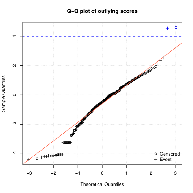
Figure 1: Normal QQ plot of outlying scores with a threshold. The symbols ”o” and ”+” indicate the event and censored observations, respectively. The solid red line passes through the first and third quartiles and the dotted blue line is a threshold to detect outliers. The observations above the threshold are claimed as outliers.

The residual-based algorithm with a coefficient $k_{r}$ of 1.5 can be applied using method = "residual" with k_r = 1.5 as follows:

> fit2 <- odc(Surv(log(time), status) ~ meta, data = ebd, method = "residual", k_r = 1.5)> plot(fit2)> fit2

     Outlier Detection for Censored Data Call: odc(formula = Surv(log(time), status) ~ meta, data = ebd, method = "residual",    k_r = 1.5) Algorithm: Residual-based algorithm (residual) Model: Locally weighted censored quantile regression (Wang) Value for cut-off k_r:  1.5 # of outliers detected:  9 Outliers detected:    times delta (Intercept) meta residual sigma Outlier57   4.80     0           1    2     1.63   1.6       *80   5.04     1           1    0     1.64   1.6       *189  5.38     0           1    0     1.98   1.6       *191  5.20     0           1    0     1.80   1.6       *233  5.29     0           1    1     2.00   1.6       *296  4.86     1           1    4     1.90   1.6       * 6 of all 9 outliers were displayed. Nine observations by k_r = 1.5 were selected as outliers, six of which are shown in the above output. All the outliers detected can be displayed by running fit2@outlier.data.

The boxplot algorithm with a coefficient $k_{b}$ of 1.5 can be applied using method = "boxplot" with k_b = 1.5, as follows:

> fit3 <- odc(Surv(log(time), status) ~ meta, data = ebd, method = "boxplot", k_b = 1.5)> plot(fit3)> fit3

     Outlier Detection for Censored Data Call: odc(formula = Surv(log(time), status) ~ meta, data = ebd, method = "boxplot",    k_b = 1.5) Algorithm: Boxplot algorithm (boxplot) Model: Locally weighted censored quantile regression (Wang) Value for cut-off k_b:  1.5 # of outliers detected:  1 Outliers detected:    times delta (Intercept) meta   UB Outlier346  4.48     0           1    9 4.32       * 1 of all 1 outliers were displayed. The boxplot algorithm with a coefficient $k_{b}$ of 1.5 detected only one outlying point. The 346th observation detected was also detected by both the scoring and residual-based algorithms. The boxplot algorithm with a coefficient $k_{b}$ of 1.0 yielded the same result as the scoring algorithm with a threshold $k_{s}$ of 4.0; that is, the 346th and 327th observations were detected. Lastly, the coef-method function can be used to give the estimated 10th, 25th, 50th, 75th, and 90th quantile coefficients as follows:

> coef(fit)

               q10    q25    q50    q75    q90(Intercept)  1.609  2.549  3.332  4.190  5.037meta        -0.039 -0.064 -0.091 -0.121 -0.138

6 Conclusion

In this paper, we proposed three algorithms to detect outlying observations on the basis of censored quantile regression. The outlier detection algorithms were implemented for censored survival data: residual-based, boxplot, and scoring algorithms. The residual-based algorithm detects outlying observations using constant scale estimates, and therefore, it tends to select relatively many observations to achieve a high level of sensitivity in identifying outliers. Thus, this algorithm is effective when high sensitivity is essential. The results of our simulation study imply that the boxplot and scoring algorithms with censored quantile regression are more effective than the residual-based algorithm when considering sensitivity and specificity together. The residual-based and boxplot algorithms require a pre-specified cut-off to determine whether observations are outliers. Thus, these two algorithms are useful if a cut-off can be provided in advance. Moreover, the boxplot algorithm can be applicable when a single covariate exists. The scoring algorithm is more practical in that it provides the outlying magnitude or deviation of each point from the distribution of observations and enables the determination of a threshold by visualizing the scores; thus, this scoring algorithm is assigned as the default in our package.

All the algorithms were implemented into our developed R package OutlierDC, which is freely available via Comprehensive R Archive Network (CRAN). The odc function yields the result of outlier detection by the residual-based, boxplot, or scoring algorithm. The resulting object can be used for generic functions such as show, update, plot, and coef. The help page for the odc function contains several examples for use in algorithms. These can be easily accessed by the example(odc) command. In our package, there are several options that users need to choose. For convenience, the most effective and practical choice is assigned as the default for each option. Thus, first-time users can run our package easily by following the illustration without a deep understanding of the presented algorithms.

7 Acknowledgements

This research was supported by the Basic Science Research Program through the National Research Foundation of Korea (NRF) funded by the Ministry of Education, Science and Technology (2010-0007936).

References

- Abuzaid et al (2012) Abuzaid AH, Mohamed IB, Hussin AG (2012) Boxplot for circular variables. Computational Statistics 27(3):381–392
- Aggarwal (2013) Aggarwal CC (2013) Outlier Analysis. Springer, New York, NJ
- Alshalalfa et al (2012) Alshalalfa M, Bismar TA, Alhajj R (2012) Detecting cancer outlier genes with potential rearrangement using gene expression data and biological networks. Advances in bioinformatics 2012
- Atkinson et al (2010) Atkinson AC, Riani M, Cerioli A (2010) The forward search: Theory and data analysis. Journal of the Korean Statistical Society 39(2):117–134
- Béguin and Hulliger (2004) Béguin C, Hulliger B (2004) Multivariate outlier detection in incomplete survey data: the epidemic algorithm and transformed rank correlations. Journal of the Royal Statistical Society: Series A (Statistics in Society) 167(2):275–294
- Chaloner and Brant (1988) Chaloner K, Brant R (1988) A bayesian approach to outlier detection and residual analysis. Biometrika 75(4):651–659
- Cho et al (2008) Cho H, Kim Y, Jung H, Lee S, Lee J (2008) OutlierD: an R package for outlier detection using quantile regression on mass spectrometry data. Bioinformatics 24(6):882–884
- Eo et al (2012) Eo S, Pak D, Choi J, Cho H (2012) Outlier detection using projection quantile regression for mass spectrometry data with low replication. BMC Research Notes 5(1):236
- Han (2013) Han J (2013) Outlier detection for temporal data: A survey. IEEE Transactions on Knowledge and Data Engineering 25(1):1
- Hankey et al (1999) Hankey B, Ries L, Edwards B (1999) The surveillance, epidemiology, and end results program a national resource. Cancer Epidemiology Biomarkers & Prevention 8(12):1117–1121
- Hoaglin et al (1986) Hoaglin DC, Iglewicz B, Tukey JW (1986) Performance of some resistant rules for outlier labeling. Journal of the American Statistical Association 81(396):991–999
- Koenker (2013) Koenker R (2013) quantreg: Quantile Regression. R package version 4.98
- Lu et al (2003) Lu CT, Chen D, Kou Y (2003) Algorithms for spatial outlier detection. In: Data Mining, 2003. ICDM 2003. Third IEEE International Conference on, IEEE, pp 597–600
- Nardi and Schemper (1999) Nardi A, Schemper M (1999) New residuals for cox regression and their application to outlier screening. Biometrics 55(2):523–529
- Peng and Huang (2008) Peng L, Huang Y (2008) Survival analysis with quantile regression models. Journal of the American Statistical Association 103(482):637–649
- Portnoy (2003) Portnoy S (2003) Censored regression quantiles. Journal of the American Statistical Association 98(464):1001–1012
- R Core Team (2012) R Core Team (2012) R: A Language and Environment for Statistical Computing. R Foundation for Statistical Computing, Vienna, Austria
- SAS Institute Inc. (2008) SAS Institute Inc (2008) SAS/STAT 9.2 User’s Guide: the QUANTREG Procedure (Book Excerpt). SAS Institute Inc., Cary, NC
- Sawant et al (2012) Sawant P, Billor N, Shin H (2012) Functional outlier detection with robust functional principal component analysis. Computational Statistics 27(1):83–102
- Schwager and Margolin (1982) Schwager SJ, Margolin BH (1982) Detection of multivariate normal outliers. The annals of statistics 10(3):943–954
- Sim et al (2005) Sim CH, Gan FF, Chang TC (2005) Outlier labeling with boxplot procedures. Journal of the American Statistical Association 100(470):642–652
- Sun and Genton (2011) Sun Y, Genton MG (2011) Functional boxplots. Journal of Computational and Graphical Statistics 20(2)
- Therneau (2012) Therneau T (2012) A Package for Survival Analysis in S. R package version 2.36-14
- Tukey (1977) Tukey J (1977) Exploratory data analysis. Addison-Wesley, Reading, MA
- Wang and Wang (2009) Wang H, Wang L (2009) Locally weighted censored quantile regression. Journal of the American Statistical Association 104(487):1117–1128
- Weisberg (2005) Weisberg S (2005) Applied linear regression, 3rd edn. John Wiley & Sons, Hoboken, NJ
- Zeileis and Croissant (2010) Zeileis A, Croissant Y (2010) Extended model formulas in R: Multiple parts and multiple responses. Journal of Statistical Software 34(1):1–13
- Zimek et al (2012) Zimek A, Schubert E, Kriegel HP (2012) A survey on unsupervised outlier detection in high-dimensional numerical data. Statistical Analysis and Data Mining 5(5):363–387