On User Availability Prediction
and Network Applications
Abstract
User connectivity patterns in network applications are known to be heterogeneous, and to follow periodic (daily and weekly) patterns. In many cases, the regularity and the correlation of those patterns is problematic: for network applications, many connected users create peaks of demand; in contrast, in peer-to-peer scenarios, having few users online results in a scarcity of available resources. On the other hand, since connectivity patterns exhibit a periodic behavior, they are to some extent predictable. This work shows how this can be exploited to anticipate future user connectivity and to have applications proactively responding to it. We evaluate the probability that any given user will be online at any given time, and assess the prediction on six-month availability traces from three different Internet applications. Building upon this, we show how our probabilistic approach makes it easy to evaluate and optimize the performance in a number of diverse network application models, and to use them to optimize systems. In particular, we show how this approach can be used in distributed hash tables, friend-to-friend storage, and cache pre-loading for social networks, resulting in substantial gains in data availability and system efficiency at negligible costs.
Index Terms:
Predictive models, peer-to-peer computing, user availabilityI Introduction
Internet application workloads, being direct consequence of human activity, are very often characterized by highly variable patterns of requests; daily, weekly and seasonal patterns are ubiquitous in these applications, and have been recorded in traces of file-sharing, instant messaging, and distributed computing [1, 2, 3, 4, 5, 6]. Despite this fact, in many cases system design and modeling are performed without accounting for periodic request patterns that are often very strong.
The fact that user behavior is often correlated – in the sense that many users will behave similarly at the same time – is especially problematic. “Flash crowds” – i.e., simultaneous requests from many users at the same time – create strains on application resources; on the other hand, the fact that many users can go offline at the same time creates problems in peer-to-peer applications, since sudden and unexpected variations of available resources can happen. Many applications are designed according to simple models of user availability (e.g., modeling availability with a uniform probability for all users [1] or using simple Markovian models [7]) that fall short when modeling the complexity of human behavior; in real world scenarios, then, systems should be largely over-dimensioned in order to avoid potential problems.
Over-dimensioned systems can re-use excess resources in other ways. However, alternative usages (which need to be exploitable at any moment in time) are likely to provide less added value than those for which the system was designed in the first place. In addition, even when elastic resource allocation is possible, it is not necessarily instantaneous. For example, spawning and booting new virtual machines can take some time – in particular in cases of heavy system load. Systems able to predict request spikes can respond proactively to increases in system load – allocating new resources when load is still tolerable – rather than reactively.
In this work, we model user availability, i.e. whether users are online, using past statistics of their uptime in order to capture idiosyncratic behavior characteristics and obtain personalized predictions for each of them. This allows us to design systems that respond proactively to user uptime. We focus on characterizing future user availability with an individualized, long-term, probabilistic statistical model: a (scalable) system which assigns a probability to the event of any user being online at any time in the future.
We evaluate our long-term predictions in different network applications. We use three different datasets (Section III) containing traces of user availability spanning a time frame of about six months in the domains of instant messaging, file sharing, and home gateways.
Our statistical model (Section IV) adopts logistic regression to combine several features capturing different periodic trends of individual and global user availability patterns. By taking a probabilistic approach, we are also able to quantify the uncertainty in the estimation of model parameters and account for it in predicting user availability. This is often useful: for example, evaluating that a user will be online with probability 0.6 while for another user the probability is 0.9 can allow applications to make different decisions for the two users; conversely, a boolean predictor that would just output “online” for both cannot allow for such differentiations.
The scalability of our approach allows us to assess the performance of our predictions on datasets of several weeks and with a large number of users (Section V). The characteristics of the dataset impact the quality of predictions that can be made, but our model remains consistently useful in all cases; moreover, the quality of predictions does not decrease substantially over time, even after several weeks. The most relevant features are those capturing individual and periodic long-term user behavior; this suggests that our approach can be adopted whenever users have a peculiar behavior which is stable over time (e.g., online social networks, accesses to email servers, TV/radio consumption even over IP, etc.).
Metrics for prediction quality, however, are not sufficient to understand the impact that our method could have on system design. We show that in Section VI, by presenting three use cases in which our approach can be adopted to predict system behavior and performance, and can be used to guide system choices. By driving node placement and data placement respectively in a distributed hash table and a friend-to-friend storage application, resource usage can be reduced because it is not necessary to perform excessive data replication to obtain a desired level of data availability; by adopting connectivity predictions in social networks, the efficiency of cache pre-fetching can be significantly improved.
Within all classes of user behavior that can be predicted, in this work we focus on user uptime because i) traces are availabile and ii) as mentioned above, we can provide concrete examples of exploiting availability prediction. In Section VII, we conclude by mentioning other kinds of user behavior and application use cases that could benefit from an approach similar to the one described in this document.
II Related Work
Patterns of user availability are important in a large class of applications since they impact the demand of resources; they are essential in peer-to-peer (P2P) systems, where they also determine the offer of available resources in the system. It is therefore unsurprising that this issue has attracted particular interest in the P2P literature, as we discuss next.
User Availability Modeling and Prediction
Various papers [4, 8, 9] focused on characterizing session length, i.e. the amount of time a user will spend online after connecting. Predicting session length is useful for cases where a node’s disconnection triggers expensive operations, such as data maintenance in distributed hash tables [10]; these techniques do not leverage on periodicity, but rather model session length with a probability distribution which is independent from the moment in which the session begins. Our analysis is complementary to this, since we focus on being able to predict connectivity patterns in the long term.
Daily and weekly periodic behavior is a known feature of essentially any trace of applications whose workloads depend on human factors. This behavior has been reported, for example, in file-sharing applications [1, 2, 5, 9], instant messaging [3], and distributed computing [4]. In addition to merely recognizing the presence of periodicity, in this work we exploit it in order to enhance the quality of our predictions.
Mickens and Noble [5] predict future node uptime on several traces, including cases where availability patterns are dictated mostly by technical reasons such as failures (e.g., availability traces of nodes in PlanetLab). We implemented this approach, and we devote Section V-A to show how our approach outperforms it in terms of prediction accuracy, scalability, and expressivity of the output.
Applications
Understanding availability is fundamental in P2P storage applications, where data is uploaded redundantly to various peers; when enough of them are online, data is accessible by other peers. In several cases, availability is modeled under the assumption that the probability that any node is online at any time is constant. In order to avoid problems due to correlated downtimes, this probability has to be estimated very conservatively, resulting in a dramatic system overprovisioning (e.g., Bhagwan et al. [11] adopt the lowest observed fraction of connected users in the history of the system). In some approaches [5, 12], heterogeneity in availability traces is exploited to increase load on nodes with higher availabilities and optimize system performance. These approaches inevitably result in an imbalance on requested resources, penalizing the most available nodes. Unlike them, we show that better performance can be obtained without requiring additional resources from any node. Pamies-Juarez et al. [13] show how better system performance can be obtained without requiring usage of more resources from more available nodes, but they validate their findings with synthetic experiments that do not account for correlation in uptime, which is extremely problematic for the envisioned storage application. Finally, Kermarrec et al. [14] propose an ad hoc method for data placement accounting for periodic availability patterns. In Section VI, we show two use cases where optimization strategies driven by availability predictions applied to peers can substantially optimize data availability; in our scenario, our method largely outperforms the one by Kermarrec et al.
User request patterns have regularities that can be used to anticipate future user behavior and plan capacity accordingly. Gürsun et al. [15] use a simple model of these regularities to predict the total number of users that will request an individual video file on YouTube the next day. With respect to their work, we perform our predictions on a personalized basis, and several weeks in advance. In Section VI-C we show how our predictions can be used to drive a pre-fetching strategy for newsfeeds in social networks: in this case per-user predictions are needed, and non-personalized predictive approaches [16, 17] cannot be applied.
Regularities of user requests are not limited to temporal patterns: user location and social connectivity can also be used to drive smart caching and pre-fetching strategies [18, 19]. While considering these additional features is not within the scope of this work, these efforts confirm that proactive approaches to system design that anticipate user behavior are feasible and efficient. We think that a probabilistic approach similar to the one we present here could also be applied in the design of systems such as those ones.
III Datasets
We evaluate our predictions on three availability traces (i.e., informations about when users are online) from Internet applications. These traces share three key properties that make them suitable for our study.
First, they comprise thousands of users and they are long enough (at least six months each) to let us test the quality of predictions over several weeks.
Second, uptime depends on which motivations users have to connect: the three datasets we use allow us to examine cases in which the different nature of the application results in different motivations for users to be online. In addition to the simple fact that users have to be connected to use the service, in the Kad dataset there is an incentive mechanism that encourages users to stay online even more.
Third, the traces we use present low or no sampling bias [20, 21], since they are essentially uniform or full samples of the users in each system.
To obtain a uniform duration between datasets, we consider only the first 24 weeks. We use the first 18 weeks to extract our features, and the remaining 6 weeks to test the predictive performance of our model: more details can be found in Section IV. We expressed each trace as an availability matrix by sampling the availability of each user with a period of one hour. We denote if user is available at timeslot , and otherwise.
The GW and Kad datasets are publicly available; since IM may contain potentially sensitive informations about user behavior, we cannot commit on making it public. To help reproducibility and re-use of our experiments, our source code is available in a public GIT repository.111https://bitbucket.org/matteodellamico/uptime-prediction
III-A IM – Instant Messaging
The IM trace is extracted from the server logs of an instant messaging server in Italy; one of the authors is an administrator of the server. The trace contains the complete log of connection/disconnection events on the server in the period between January 10, 2010 and June 27, 2010; distinct users connected to the server in that time-frame. We denote a user as “online” if at least one client software is logged in with the user’s credentials, regardless of the status set in the client (e.g., available, busy, invisible…).
In this system, very strong daily patterns are observable. We attribute this to two reasons: first, most users live in the same timezone; second, they are likely to go online whenever they are in front of their computer, in order to be reachable.
In the period of May 18–20, a large number of accounts was registered by automatic tools; such accounts, being non-human, had connectivity patterns that were fundamentally different from those observed in the rest of the trace. Separating human and non-human behavior with means such as CAPTCHAs and characterizing online behavior of automated tools are both outside the scope of this work. This phenomenon, however, does not affect the results shown in this work: these accounts were registered only after our training period (i.e., in the last six weeks of the trace). Availability predictions for them have therefore neither been generated nor tested.
III-B GW – Gateways
The GW trace has been extracted by Serge Defrance et al. [22]. It comprises traces from residential gateways of the French ISP Free having a fixed IP address, and it was obtained by pinging each gateway every 10 minutes. The set of IP addresses was chosen randomly within the address space allocated for these gateways, and a gateway was included in the trace if it had answered to the ping message at least once. In this work we consider availabilities in the 24-week interval between June 29, 2010 and December 24, 2010; four aberrations where most users appear offline due to measurement artifacts are present in the dataset and are acknowledged by the authors.222http://www.thlab.net/~lemerrere/trace_gateways/
The gateways provided by Free offer access to telephone services, TV and DVR in addition to Internet access; for this reason many users keep their gateways almost always on. As a result, the average percentage of connected users is 86% over the trace. Daily and weekly periodic behavior is still present, with a number of users that disconnect their gateways mostly during the night.
III-C Kad
The Kad trace has been extracted by Steiner et al. [6], measuring the connectivity on nodes on the Kad distributed hash table, which is used by clients of the popular eDonkey2000 network. In Kad, nodes are identified by a randomly generated 128-bit identifier called Kad ID; the trace contains the result of a zone crawl resulting in the availability trace (sampled every 5 minutes) of all the nodes sharing a common 8-bit prefix appearing online in a six-month period. We consider availability data between September 23, 2006 and March 10, 2007.
In the eDonkey2000 network, users are implicitly motivated to stay online when they are downloading files; moreover, there is an elaborate credit-based incentive scheme [23] designed to reward users that stay online and upload data to peers with faster download speeds.
III-D First Observations

In Figure 1, we show the distribution of the per-user average availability in each dataset (i.e., the distribution of the fraction of time each user spends online). Because of the applications’ nature, these values are drastically different. It is interesting to note that, even though an incentive scheme has been devised in order to convince users to stay online more often, the Kad trace is the one with lowest availability values overall. It appears that the incentive mechanism present in the network has a limited impact, and that the very nature of the applications that encourages users to stay online to remain reachable to receive instant messages (IM) or phone calls (Kad) plays a much stronger role.
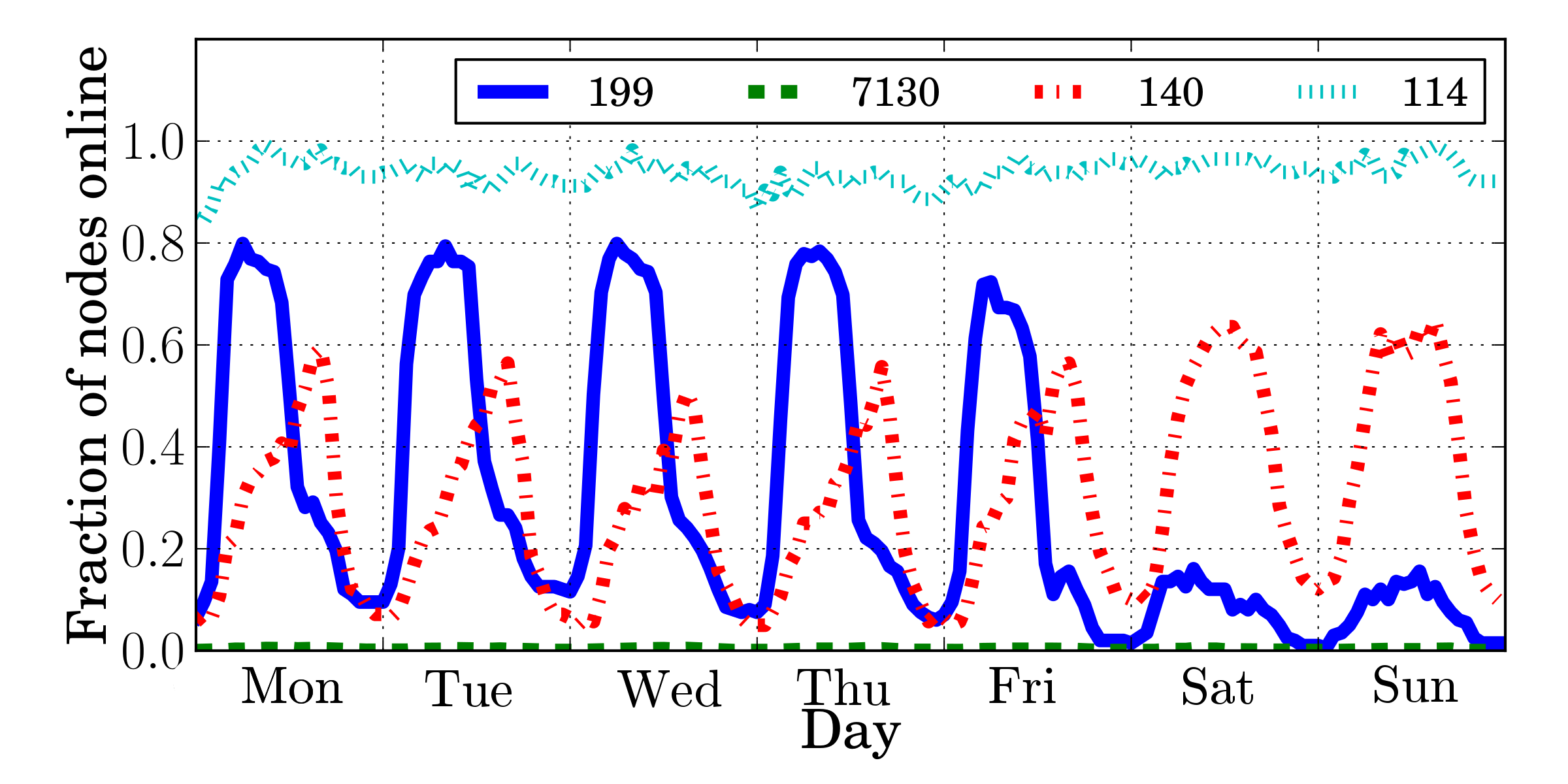
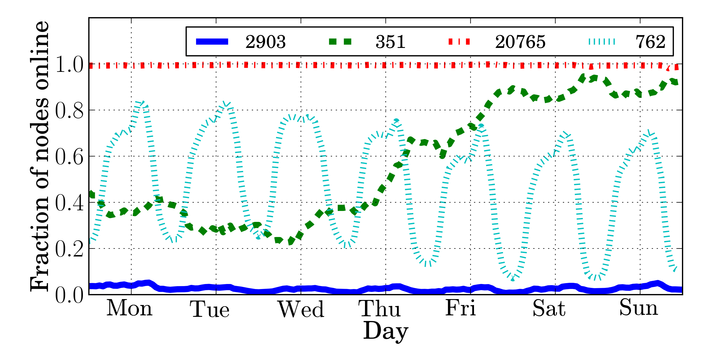
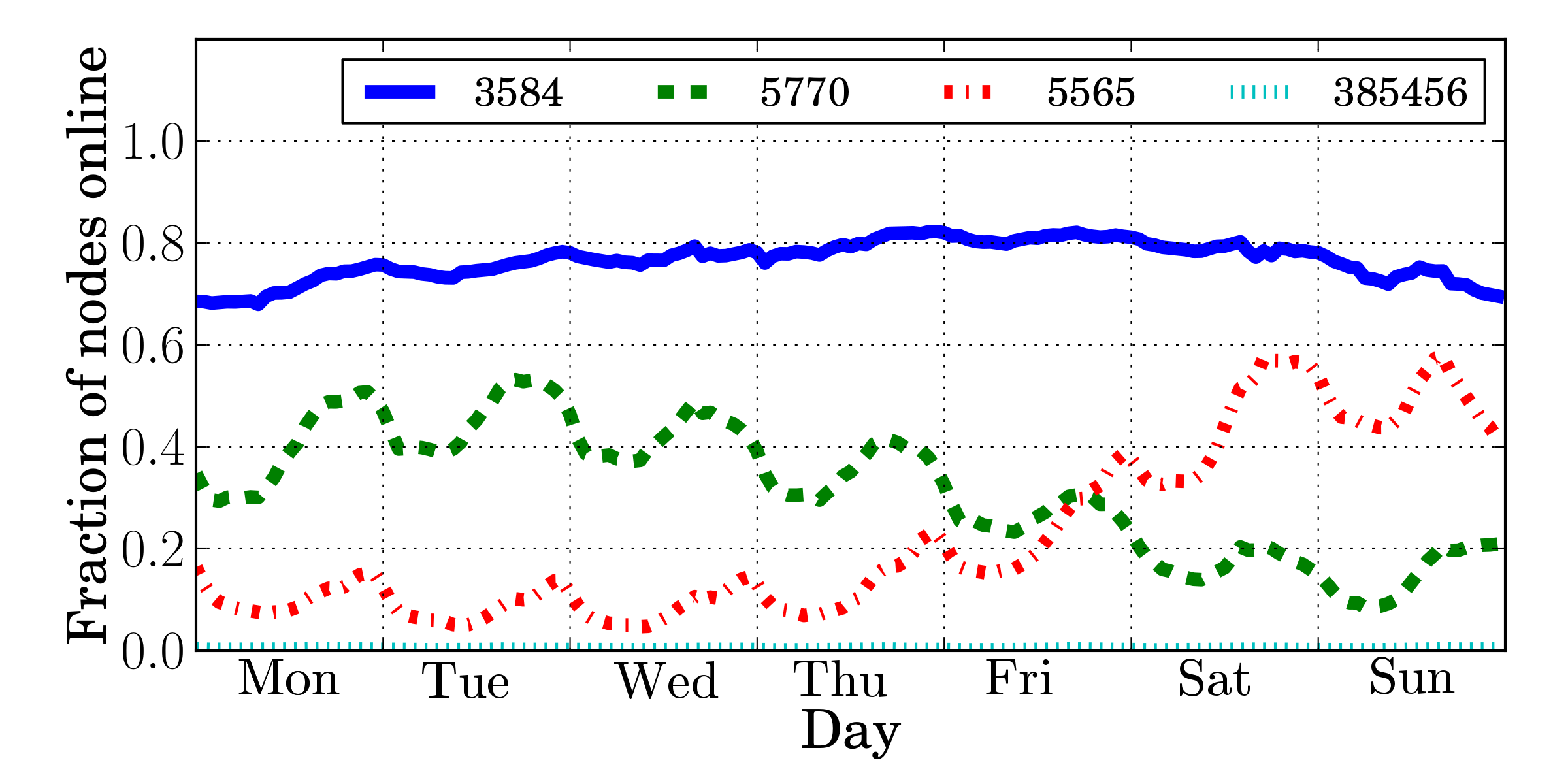
In Figure 2, we highlight the diversity of per-user availability in each dataset. We took a sample week from each trace, and sampled the availability of each user with a granularity of one hour, to obtain a matrix where lines represents users and columns timeslots. Each cell indicates whether the user was online or not at that time.
We performed -means clustering on the lines of this matrix, resulting in a clustering of users (we chose for plot readability), and we plot the average number of per-cluster available users. Each line corresponds to a cluster; in the legend, we report the number of users belonging to each cluster.
From Figure 2, we can obtain an intuitive grasp of the behavior of some representatives groups of users in the cluster. In all cases there are clusters of users who are mostly on and mostly off, and others with different inclinations to connect: mostly during weekdays or mostly during weekends. The size of these clusters (shown in the legend) can explain the distribution of per-user average availability values shown in Figure 1.
In the IM trace, it is interesting to note that some users tend to connect during office hours (blue cluster), and others in free time (early night and weekends, red cluster). The clustering results show that such a phenomenon is less common for GW and Kad, where the -means clustering instead captured groups of users whose availability pattern changed during the week under scrutiny (green cluster for GW, red and green clusters for Kad).
In summary, our datasets represent three different types of network applications with markedly different user behavior; moreover, IM clients [24], home gateways [25, 22], and file-sharing clients [6] are all popular platforms for running peer-to-peer applications, making these datasets ideal to test the peer-to-peer application use cases shown in Sections VI-A and VI-B.
IV Our Model
In this section we introduce the model that we use for predicting user availability. We start with a set of features that identify global and personalized periodic trends, and combine them in a classifier, as we will see shortly. In this work we adopt a fully probabilistic classifier based on logistic regression, as it provides high descriptive power and is quite flexible. We split the data sets in four non-overlapping consecutive periods A, B, C, and D, each of duration of six weeks. Inference on the parameters of the classifier is carried out using A to compute the features and B to obtain the corresponding labels. We use C and D to assess the predictive performance of the probabilistic classifier. Now C is used to construct features and D to obtain labels against which classification performance is assessed.
The proposed procedure avoids any issues with reusing the same data for inference and for assessing the quality of the classifier, and preserves temporal information in the process as if we were to apply this procedure in a real scenario. Although this does not allow to evaluate some sort of cross-validation error, we report results on three different scenarios comprising thousands of users, that substantiate the hypothesis that patterns of availability are largely predictable.
In several cases stemming from P2P applications [26, 24], it is most interesting to consider “superpeers”, which are nodes with a relatively high availability: for example, in the Wua.la distributed storage application [27], data is stored on peers that have spent at least an average of 4 hours per day online in the past week. Mirroring this latter requirement, we created restricted filtered datasets containing nodes that spend on average at least 4 hours per day online. This filtering is performed on period A for both period A and B, and on period C for periods C and D: in other words, a node will appear in the filtered dataset in period B (resp. D) if it has been available on average at least four hours per day in period A (resp. C). This process resulted in selecting 405 users in the IM dataset for the A-B periods, and 408 nodes in the C-D periods. For GW, the selected nodes are 22,620 (A-B periods) and 23,184 (C-D). For Kad, they are 11,472 (A-B) and 12,522 (C-D).
Filtered datasets allow us to evaluate the predictor quality for use cases of interest ignoring easily predictable, mostly-offline users. We use the filtered datasets for our application use cases in Sections VI-A and VI-B.
IV-A Features
User availability follows periodic daily and weekly trends which affect the whole system. Moreover, each user has his/her own particular daily and weekly trends (e.g. being more or less likely to connect on nights and on weekends, as shown in Figure 2), as well as different likelihood to be online at all (see Figure 1). We designed a set of features aimed to capture each of these trends.
We are interested in creating a prediction for each user and each timeslot in the future. For a user and a timeslot , we identify a set of observations that are related to the trend we want to identify with the feature at hand, and we simply count the numbers and of observations in which we find nodes respectively online and offline. We then return as an output of -th feature the value
These values can be seen as the expected value of the posterior of a Bernoulli trial assuming a flat prior . We point out that it is computationally trivial to update these features when new observations become available.
We define five different features, which differ by set of users considered (individual or global) and by periodicity (daily, weekly, and flat). Features differ only by the definition of the set of observations which is taken into account in order to compute :
-
1.
Global daily. Observations of all users, same time of day of (e.g., if is at 9:00 AM, observations taken into account will be at all days at 9:00 AM).
-
2.
Global weekly. All users, same time of day and same day of week of (e.g., if is on a Monday at 9:00 AM, observations taken into account will be at all Mondays at 9:00 AM).
-
3.
Individual flat. Exclusively user , any observation in the training set.
-
4.
Individual daily. User , same time of day of .
-
5.
Individual weekly. User , same time of day and same day of week of .
It is possible to consider additional features accounting for periodic behavior. We observed a sharp decrease in the number of connections in holiday periods (i.e., the month of August and the Christmas period). Unfortunately, our traces are not long enough to allow us taking into account seasonal variations. We consider it more than reasonable to assume, however, that even longer traces would result in increased accuracy.
In addition, we empirically observed that public holidays result in availability patterns that are similar to those of weekends. Unfortunately, since our traces comprise users from different countries, it is difficult to define precisely which days are public holidays.
IV-B Logistic Regression
The five features above are able to capture different aspects of patterns of availability, and we are interested in combining these pieces of information to accurately predict future user availability. Moreover, we aim to assess the relative importance of the five features in doing so. We propose a fully probabilistic logistic regression classifier [28]. Adopting a probabilistic classifier yields a probability of users to be online at a given time. This reflects in the possibility to obtain a degree of how certain the classifier is on the availability of users that can be exploited in network applications.
In logistic regression, and more in general in a classification problem, a set of labels is associated with a set of samples , each described by a set of features so that . In our application the labels represent , that is the availability of user at time , and is the corresponding set of five features . The logistic regression classifier models the labels as conditionally independent, and as draws from a Bernoulli distribution with probability of “success” given by:
where denotes the logistic function . Note that we have introduced an intercept term in the linear combination to allow for a term in the combination independent from the features. In order to keep the notation uncluttered, we define the set of weights of the combination together with the intercept term as , and with abuse of notation we redefine so that the linear combination becomes . Also, we define and similarly . Finally, let be the matrix obtained by stacking the vectors by row.
The goal of a classification approach is to tune or infer the parameters based on past user availability data, and use this to predict future user availability. It is worth noting here that, once the parameters are inferred from data, they offer an interpretation of the relative importance of the different features in discriminating between the classes. We now report the approach that we take to infer the parameters and explain how we predict future user availability.
IV-B1 Bayesian Inference
In this work we take a Bayesian approach to infer the parameters of the logistic regression classifier. The motivation for doing so is that the Bayesian approach offers a sound quantification of uncertainty in parameter estimates and in predictions, as demonstrated in several applications [29]. In a probabilistic setting, the predictive distribution for a new test sample is obtained via the following marginalization:
| (1) |
Equation 1 requires the so called posterior distribution over after observing and . Note that this expression is quite appealing as the uncertainty on the parameters a posteriori is effectively averaged out when predicting future availability. As a result, predictions no longer depend on model parameters. This is in contrast to what would happen if we optimized the parameters, obtaining say , that would lead to predictions of the form that are conditioned on a specific choice of . The core of quantification of uncertainty in parameter estimates and predictions is therefore in the posterior distribution over . By Bayes theorem, is proportional to , namely the product of the likelihood of the observed availability given the parameters, and the prior distribution over the parameters. The log-likelihood of the observations given the parameters is
We assign a Gaussian prior over with mean and features . In this work we assume a rather flat prior over ; in particular, we set and with . Given the amount of data and the variance of the prior, the Gaussian assumption is not restrictive, but has the advantage of being simple to deal with.
Given the form taken by the likelihood in the logistic regression model, it is not possible to obtain the posterior distribution on in closed form, and it is therefore necessary to resort to some approximation. It is possible to approximate the posterior distribution using deterministic approximations [28, 30], or employ a Markov chain Monte Carlo (MCMC) approach to obtain samples from the posterior distribution [31]. Here we employ a deterministic Gaussian approximation technique called Laplace Approximation.
IV-B2 Laplace Approximation
The LA algorithm is a deterministic technique that approximates a function using a Gaussian. This approximation places the approximating Gaussian at the mode of the target distribution and sets its covariance to the covariance of the target distribution [28]. Although it can be argued that a Gaussian approximation can be very poor when the target distribution is far from being Gaussian, in the limit of infinite data the posterior distribution will tend to a Gaussian (see, e.g., [32] for further details). In this application we are dealing with very large amounts of data (in the order of millions) and therefore the LA is appropriate in characterizing the uncertainty on parameter estimates. Moreover, given that the complexity of the whole algorithm is linear in the number of data (see below), it scales well for large data sets.
In this work, we make use of the iterative Newton-Raphson optimization strategy to carry out the Gaussian approximation, as it is commonly employed in logistic regression. The Newton-Raphson optimization iteratively uses gradient and Hessian of the logarithm of the target function to locate its mode. Denoting with the update of the parameters after one iteration, the Newton-Raphson formula is
This update is repeated until the gradient vanishes, which in practice is assessed by checking that the norm of the gradient is less than a given threshold. In the case of logistic regression, the update equation is:
where we have defined as a diagonal matrix with . After convergence, we have an approximation , where is the value of at the end of the optimization and is the covariance of evaluated at . The complexity of each update of is linear in the number of samples , and cubic in the number of parameters due to the inversion of a matrix. Given that in our application , the LA results in a very fast method (reported in Algorithm 1) for inferring the parameters of the model.
Note that the probabilistic framework allows one to carry out the inference by processing data in batches. In particular, this can be accomplished by simply treat the posterior on after processing one batch of data as the prior for before processing a new batch of data. We resorted to this option in the case of the KAD data set only, where the data were split in ten batches of several tens of millions of samples due to limitations in storing all the data into memory.
Input: Data: , - Prior: - stopping criterion
Output: Gaussian posterior:
while
return
IV-B3 Predictions
The predictive distribution is obtained by solving the integral in Eq. 1, where now we have a Gaussian approximation to . Defining and , the predictive distribution results can be approximated by
The complexity of evaluating this expression (in Algorithm 2), once and are available, is linear in the number of parameters.
Input: Data: , - Gaussian posterior: - test data:
Output: Prediction
return
IV-C Scalability
To compute predictions, our method performs two steps: feature extraction and logistic regression. Computation is lightweight: both steps scale linearly and they are dominated by the speed at which input data is read and parsed. The feature extraction component, which is the one dealing with the largest input, can be easily parallelized; the logistic regression component, in our prototype implementation, can handle the around 100 million data points of the GW dataset in around one minute.
V Prediction Accuracy
We report two measures of performance for our classifier, namely the Area Under the Curve (AUC) of the Receiver Operating Characteristic (ROC) and the geometric mean of the likelihood on test data (GM).
AUC measures how well a probabilistic classifier balances true and false positives, with the optimal value of 1 corresponding to the case where all true positives are associated probabilities larger than any true negative.
The GM score, instead, is calculated as
where is the likelihood of the availability observation for user and time given a predicted probability of : if , else . GM is a value between and and it is larger for classifiers that assign correct predictions with high confidence, measured through the predictive probability. GM complements the AUC metric by accounting for the confidence level of the output of the classifier.
| IM | GW | Kad | |||||||
| AUC | GM | (st. dev.) | AUC | GM | (st. dev.) | AUC | GM | (st. dev.) | |
| ALL | .939 | .785 | .916 | .807 | .826 | .933 | |||
| Individual daily | .938 | .779 | 0.47 (.01) | .912 | .806 | 1.04 (.00) | .826 | .933 | 0.38 (.00) |
| Individual flat | .914 | .756 | 0.52 (.01) | .915 | .805 | 0.17 (.00) | .816 | .931 | 0.12 (.00) |
| Individual weekly | .918 | .776 | 0.60 (.01) | .896 | .803 | 0.04 (.00) | .755 | .931 | 0.11 (.00) |
| Global daily | .583 | .617 | -0.06 (.01) | .522 | .659 | 0.02 (.00) | .532 | .914 | -0.06 (.01) |
| Global weekly | .593 | .618 | 0.29 (.01) | .523 | .659 | -0.01 (.00) | .530 | .914 | 0.14 (.01) |
| IM filtered | GW filtered | Kad filtered | |||||||
| AUC | GM | (st. dev.) | AUC | GM | (st. dev.) | AUC | GM | (st. dev.) | |
| ALL | .901 | .666 | .845 | .823 | .730 | .599 | |||
| Individual daily | .890 | .652 | 0.54 (.01) | .834 | .822 | 0.71 (.00) | .728 | .599 | 0.65 (.00) |
| Individual flat | .815 | .611 | 0.28 (.01) | .841 | .821 | 0.18 (.00) | .691 | .589 | 0.05 (.00) |
| Individual weekly | .889 | .653 | 0.69 (.01) | .802 | .819 | 0.02 (.00) | .706 | .592 | 0.20 (.00) |
| Global daily | .612 | .510 | -0.17 (.01) | .539 | .762 | 0.02 (.00) | .532 | .560 | -0.21 (.00) |
| Global weekly | .627 | .513 | 0.32 (.01) | .543 | .760 | -0.01 (.00) | .534 | .560 | 0.23 (.00) |
In Table I, we show our error metrics evaluated on all datasets, for our combination of all features, along with a breakdown – for each of them – of the error metrics achievable by using a single feature in the classifier. We also report the mean and the standard deviation of the posterior over obtained by the logistic regression classifier using all the features normalized to have unit variance.
From Table I, we notice that the combined predictor is consistently better or equivalent to the other ones, showing that the combination effectively integrates information from the five features that capture basic trends. Error metrics are worse on datasets like IM filtered and Kad filtered, because they lack nodes that are mostly offline and that are therefore easier to predict. This effect is stronger on the GM metric, showing that the classifier correctly assigns very low probabilities of connectivity to nodes that are mostly offline, and it is less confident on nodes with more irregular behavior.
Table I also shows that global features consistently perform worse than individual ones: even if global trends can be clearly identified and they are useful in characterizing availability, it is clear that information about individual trends is simply more important. However, the accuracy of the classifier using all the features is higher than the one for the classifiers using a single feature, indicating that combining all the features using logistic regression is beneficial.
 |
 |
 |
 |
 |
 |
As examples of prediction performance, in Figure 3 we show predictions (dotted lines) and availability traces (solid lines) on the six weeks of test data for six typical users, two from each dataset. We selected these users to provide concrete examples of typical per-user availability patterns in the different datasets and of the way our model captures them. Since our predictor has a weekly period, we show a week of predictions and the corresponding average availability (same time of day and day of week) over the six weeks of the test set. In IM filtered, nodes frequently have strong daily periodicity (top left), often accompanied by a different behavior in the weekend (top right). These features can be easily recognized by our classifier, and this explains the particularly good performance of the predictors using only the individual daily and weekly features. In GW, nodes are frequently mostly on, with sporadic disconnections due either to failures or the measurement artifacts mentioned in Section III-B (center left); however, some users turn on their gateways only occasionally and mostly during the day (center right). This explains the good performance of predictors using individual daily and flat features. In Kad filtered, many nodes have availability patterns with varying daily periodicity (bottom): even though predictions using the “individual daily” feature perform best, the confidence level – as expressed by the GM metric – is low.
The values of in Table I are expected to be large when associated to features with high predictive quality, unless some of them convey redundant information. We only observe positive values for individual features; some negative values are instead associated to global features. The net result of this, when associated with higher positive values on the corresponding individual feature, is a case where the deviations of a node from the global trend are essentially given more importance and therefore amplified. In all cases, the standard deviation expressing the level of uncertainty associated to is low due to the amount of data processed, and guarantees that the above considerations on the relative importance of individual features are robust.

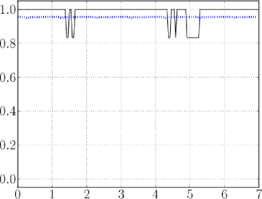
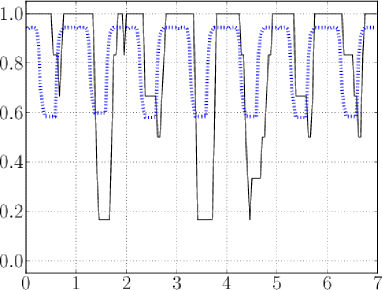
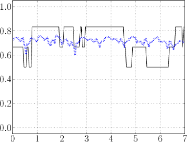
To understand the achievable false positive/false negative rates, we plot in Figure 4 ROC curves for our non-filtered datasets. The classifier has a good overall performance for IM; in contrast, it is difficult to recognize online users in Kad: this is because several users go online only sporadically and rather unpredictably. Conversely, in the GW dataset, for many users it is the downtime which is sporadic and unpredictable.
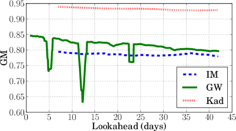
In Figure 5, we show the evolution of our error metrics over the test period, averaged on a running window of one week in order to discount daily and weekly periodic behavior – except for GW, where we use a window of one day since the clearly visible measurement artifacts reported in Section III-B would otherwise make the plot unreadable. While there is a decreasing trend – i.e., prediction quality becomes worse as predictions are made farther into the future – this decrease is only marginal: it is, indeed, possible to predict node availability even on the long run.
To summarize, the main results of this evaluation are two: first, individual periodic availability patterns enable an effective prediction of user availability even in the long term; second, the extent to which user availability is predictable is strongly dependent on the nature of the application, and in particular to the implicit and explicit incentives for availability offered by each application.
V-A Comparison with Mickens and Noble
As discussed in Section II, the method proposed by Mickens and Noble (MN hereafter) [5] is the most closely related piece of work, being the only one that explicitely tries to predict single nodes’ availability.
Before even discussing accuracy, we remark that our method has two advantages:
-
•
Scalability. Our approach is suitable for large amounts of data (e.g., the 1.6 billion data points of the Kad dataset). Conversely, MN requires training and generating predictions for a set of several predictors for each user and at each timeslot; this requires rather expensive operations (e.g., matrix inversion) for each data point. Due to these factors, we found our method to be able to process data at a speed which is faster by 4-5 orders of magnitude.
-
•
Expressivity. The output of our method is a probability of encountering a user online, while MN just outputs predictions without a probability. MN’s prediction of “online” (or “offline”) does not give any estimation over the degree of certainty of that prediction. As such, it would be impossible to use MN in the place of our approach in any of the applications we consider in Section VI.
With these considerations in mind, we proceed describing our experiments and comparing the prediction accuracy of each approach. We implemented the MN approach and used it with the parameters of [5, Section 4.1]. Due to the limited scalability of the MN method, we create a training set for both our proposal and MN where user availability is sampled every 6 hours; we train our model as before, while the training period for MN is the first 18 weeks (corresponding to periods A, B, and C of Section IV). For the smaller IM dataset, we evaluate both approaches on all users and bin them in five availability classes according to the average ratio of time spent online in the test period: . Similarly, for the larger GW and Kad datasets, we create a sample of 100 users for each one of the ten availability class . For our approach, we predict that the user will be online when the predicted probability is greater than 0.5, and offline otherwise.


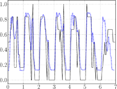
In Figure 6, we show the per-class accuracy for the predictions in each each of the availability classes. Besides noting that extreme (e.g., almost always on or off) cases are easier to predict in both cases, we note that our method obtains in most cases better performance than MN, in particular for the most frequent instances (i.e., mostly-on nodes in GW and mostly-off nodes in Kad). It can be noted that both approaches involve the combination of various features; an analysis of the possible benefits obtained by using the predictors from MN as additional features is in our plans for future work.
VI Applications
In this section, we report three examples of application use cases; they should be regarded as proofs of concept, with the goal of showing how probabilistic availability prediction can easily and effectively be integrated in a large class of realistic systems.
VI-A Node Placement on DHTs
Distributed Hash Tables (DHTs) are data structures for decentralized systems that store key/value pairs and provide an efficient lookup function. We consider a DHT holding a large amount of data (large values and/or very large quantities of key/value pairs), where information is stored on a long-term basis. In this case, data is not erased from nodes between online sessions; hence, data maintenance is required only when peers abandon the system for good. In such a situation, reaching high availability for data is very expensive in terms of resources: it is generally obtained by increasing data redundancy, which is an expensive strategy because it entails increased usage of both bandwidth and storage space on peers. Here, we show how a simple data placement policy informed by our predictions can result in higher data availability without requiring increased resource usage.
Mickens and Noble also proposed using availability prediction to optimize DHTs [5]. They considered a case where each (transient) disconnection triggers data maintenance, and proposed to alleviate the maintenance load by storing data only on the most available peers. This approach has the obvious weakness of overloading the most stable nodes, providing them an incentive to lower their availability. Differently from such approach, we focus on improving data availability without imposing any additional burden on any peer.
As in Chord [33], persistent node identifiers and hash values for keys are placed on a logical ring topology, and each key/value pair is replicated on a neighbor set of nodes, whose identifiers are the closest successors to the hash value of the key in the ring.
In general, node identifiers in DHTs are chosen randomly. We propose instead a smart policy that maximizes data availability, i.e. the fraction of time slots in which at least one peer in a neighbor set is available. For example, it would be wise to distribute two replicas of the same piece of data on a node which is often available during the day and another which is available at night.
For a given neighbor set and a set of time slots , we compute the predicted data availability (i.e., the probability that at least one node holding a replica is online) as a function of the prediction :
| (2) |
It is important to note that, by using the above formula, we are assuming that the probabilities of being available for two nodes in the same timeslot are independent. This assumption is not true when, for example, two nodes are disconnected at the same time for the same reason, such as a network outage or an external event, so this might introduce discrepancies between the predicted and observed availability distributions.
Input: prediction matrix
Output: mapping from nodes to identifiers
-
function :
return average availability on neighbor
sets of using Equation 2
# number of iterations
mapping with a random id per node
for :
for each node :
choose a random node
switching the ids of and
if :
return
Our procedure for assigning node identifiers (Algorithm 3) works by starting with a randomly assigned identifier per node, iteratively considering for each node another random one, and verifying (based on Equation 2) whether exchanging their identifiers would enhance, on average, the average predicted data availability for the involved neighbor sets. If so, their identifiers (and hence positions in the ring) are exchanged.
This policy can be easily implemented in a decentralized network, if each node starts with an availability prediction for itself. Any node can easily find candidates for exchanging positions by performing a lookup of a random key in the DHT; the availability prediction according to Equation 2 can be computed if each node shares its availability predictions with neighbors. To avoid performing too many expensive data exchanges, nodes can start accepting data once their identifier is sufficiently stable. In addition, this method can adapt over time as new nodes join and predictions get updated by continuing to look for candidates for switching positions. We assume that nodes correctly follow the protocol specified here: the design of detection and incentive mechanisms is outside the scope of this work.
Experiments
In this use case, it is recommendable to only store data on nodes with reasonably high availability: because of this, we performed these experiments on the three filtered datasets. We trained our model on the A, B and C periods, and we executed Algorithm 3 to assign node identifiers based on the D period predictions. We then measured predicted and simulated data availability according to the data placement outcome, repeating each instance of the experiment 100 times. The smallest filtered dataset is IM, with 408 users in the C and D periods. To have experiments of the same size, we chose a random sample of 408 nodes for GW and Kad in each instance of the experiment. We set a priori the neighbor set size based on the average availability of nodes in period C (0.488 for IM, 0.377 for Kad and 0.939 for GW), choosing the smallest satisfying . This corresponds to a simple uniform availability model to set redundancy aiming for similar starting conditions in the three datasets, and it results in for GW, for IM, and for Kad.
We note that all three datasets can be representative of systems where a DHT is run: an instant messaging application to look up data about users, a file-sharing application, or a P2P application running on high-availability set-top-boxes [25].
| Dataset | Random | Prediction-based | |
|---|---|---|---|
| IM | [0.77] | [0.11] | 392% |
| GW | [0.20] | [0.12] | 12% |
| Kad | [0.77] | [0.76] | 37% |
In Table II we show predicted and real data availability (i.e., the measured percentage of time slots in which at least a replica is online, averaged over each neighbor set) on the test period D (see Section IV). We report the average availability and standard deviation between instances of the experiment. In square brackets, we show the average difference between predicted and real data availability for the whole system.
From Table II, we note that our optimized data placement strategy consistently performs better than the standard random placement of nodes in a DHT; however, the increase in availability varies between the different datasets: it is most significant in IM, where the average time that a piece of data is unavailable drops from around 3.5 hours to five minutes per week; it is instead less impressive in Kad, where unavailability decreases from around eight to six hours per week. We attribute this to the difference between the datasets: when behavior is strongly periodic and easy to predict, optimized data placement results in much better availability. However, a decrease in unavailability by around a quarter is still desirable, in particular because it is obtained without any extra requirement on any node.
Reaching high availability in online storage is very expensive. Using the common availability model that assumes homogeneous storage nodes and independent failures (e.g., [11]) the required redundancy for replicated storage is directly proportional to the “number of nines” for required data availability. More formally, in that model data availability is computed as , where is the availability of any storage node and is the replication factor. It is easy to derive [34] that in order to increase data availability from to , the replication factor has to increase by a ratio of
In order to help interpreting the results of our evaluation, in Table II we provide the values of , which is determined solely by the availability values observed in our trace-driven simulations, and can be interpreted as an “equivalent redundancy increase”: i.e., the ratio of additional redundancy (and corresponding overhead in terms of bandwidth and storage space) that should be injected in the system in order to obtain an equivalent increase in availability. The improvement in IM can be considered as equivalent to an almost 400% increase in redundancy; even in the less impressive GW and Kad cases, the value of is far from negligible in terms of resource economy.
Based on the numbers in square brackets in Table II, we also notice that there is a reasonable match between predicted and real availability values. This would not happen if there were strong dependencies between availabilities of different nodes (e.g., two users disconnecting at the same time because of the same external event); as such, we believe the hypothesis of independence we used in Equation 2 to be sensible.
VI-B Data Placement for F2F Storage
We now show that our probabilistic classifier can be used to drive data placement in other declinations of P2P storage. We now consider a use case where data is still stored on users’ machines, and we still want to optimize data availability by ensuring that at least one replica of the data is online; however, we have more constraints on data placement.
Friend-to-friend (F2F) storage is an interesting instance of P2P storage. In these systems, nodes are constrained to store data only on machines owned by “friends”, with reciprocal real-world trust bonds. These trust relationships can be leveraged to obtain guarantees of dependability, privacy and security, since trusted users are unlikely to behave maliciously, selfishly or anyway deviating from the expected behavior [35, 36].
Input: prediction matrix , per-node capacity
Output: mapping such that if holds data for
-
function :
return predicted availability
for data stored in friend set
function :
# increase in availability due to
return
# random initialization of
for each node :
random friends of
for each :
# optimization
while true:
false # have changes been made?
for each node :
friends of such that
friends of such that
if :
true
if not : return
In our simplified simulation, each node has to store a data object of unitary size on friend nodes, and has a storage capacity of units, which is not sufficient to store the data for all the friends. Similarly to what we propose for DHTs in Section VI-A, we optimize the choice of nodes for which to store data in order to enhance the overall data availability. The predicted data availability can be computed again from Equation 2, using the set of friends storing replicas of a nodes’ data object as the neighbor set .
Algorithm 4 optimizes data availability as follows: each node starts by storing the pieces of data of a random subset of friends; afterwards, iteratively, each node considers erasing the piece of data that would impact less its predicted availability, and exchanging it with the one that would improve most its predicted availability. If the net effect on system availability is positive, then the switch is performed. The algorithm continues until it stabilizes, when no pieces of data are switched anymore.
Assuming once again that nodes have access to their own availability predictions and share them with friends, this algorithm is simple to implement in a decentralized system. In this case, some level of security is guaranteed by the fact that all communication happens among trusted peers. Exchanges of data can remain virtual until the algorithm has reached convergence, sparing the cost of needless uploads of data that will be subsequently erased.
Kermarrec et al. have proposed an availability-aware data placement policy for peer-to-peer storage systems called “R&A” (Random & Anti-correlated) [14], which aims to store data replicas on sets of nodes whose availability is pairwise anti-correlated. We implemented that policy in our system with constraints on resources and on eligible data holders (Algorithm 5).
Input: availability matrix , per-node capacity
Output: mapping such that if holds data for
-
function : # correlation
return
# free storage per node
mapping s.t. for each node
while :
for each node :
friends of s.t.
if : skip to next
random element of
;
if : skip to next
;
return
Experiments
| Dataset | R&A | Prediction-based | |
|---|---|---|---|
| IM | [0.04] | 23% | |
| GW | [0.13] | 47% | |
| Kad | [0.67] | 4% |
In order to have simulation results that are comparable with the DHT experiments, we have defined parameters that are analogous to the ones described in the previous section. We adopted the three filtered datasets, and samples of 408 nodes for each run of the experiment; the value describing the storage space on each node is set analogously to the redundancy value for the DHT simulation ( for IM, for GW, and for Kad). To create a synthetic model of a social network, we generated a network according to the Watts-Strogatz small-world model [37], with average degree (i.e., number of friends per user) 20 and rewiring probability 0.5.
The results on data availability for this setting are reported in Table III. By comparing it with Table II, we note that without the proposed approach we obtain a slightly lower availability with respect to the DHT after optimization; we attribute this to the lower flexibility in this scenario: while a node can take any position in the DHT, it can only store data for friends in the F2F case.
The R&A placement strategy suffers from the fact that this approach does not allow re-allocating data when poor choices have already been made, in particular for the GW case where a few pieces of data are replicated 0 or 1 times. By adopting a more accurate model of data availability and by reclaiming already allocated space in order to use it better, our proposal obtains noticeably better performance.
Discussion
The two scenarios of DHT node placement and F2F data placement bear strong similarities with each other. In both cases data availability can be modeled as a function of node availability and a design choice (respectively, choice of node identifiers and data placement). Probabilistic availability predictions make it easy to create cost functions such as Equation 2, which is fed to optimization algorithms. We point out that such an approach can be extended in several ways, including for example erasure coding, plus different application settings and storage constraint variants.
We evaluated local optimization algorithms, which optimize for predicted availability by changing only part of the solution at a time; they can get stuck in local optima. The study and evaluation of more elaborate techniques to find better solutions is outside the scope of this work, and a direction for further research.
VI-C Newsfeed Pre-Loading
We now move away from the peer-to-peer use cases, and consider a case in which we predict the availability of users behaving as clients; in this case, we use availability prediction to drive pre-loading of data for users that are most likely to connect shortly.
On social networking websites, users are often presented with some sort of “newsfeed” personalized page including recent updates by friends or followed contacts. Generating such pages involves serious scalability problems, since – due to the sheer size of databases involved – information about contacts is scattered across a large amount of servers in a data center; creating a newsfeed page requires obtaining data from a large fraction thereof. Hence, two approaches have been discussed [38] to address this issue: pull-on-demand and push-on-change.
The pull-on-demand approach queries all the relevant servers when the user requests a page: this approach requires pulling information from a large number of servers concurrently, which may result in congestion and ultimately high latency in returning the result. It could be possible to mitigate this problem with an additional layer of caching, which would however be an expensive solution having cache eviction problems [38].
Alternatively, with the push-on-change approach, a set of servers responsible for serving newsfeeds are sent user updates when they are generated. With push-on-change, information is already in a single place when the newsfeed is requested, making it more efficient to serve. Clearly, this approach entails data duplication, since each update generated by a single user will be sent to the servers responsible for each of its contacts. With push-on-change, newsfeeds are essentially pre-loaded for all users, whether or not they access the system.
Without the pretense of providing a complete system design, we sketch a hybrid solution combining both behaviors. Pull on demand is the default, as many users will connect sparingly to the system and generate few, albeit expensive, requests; the push-on-change approach is enabled for the periods of time in which a user is predicted to be more likely to connect. This approach allows to increase efficiencies for the most predictable accesses, while limiting the data duplication that would be generated by enabling push-on-change for all users.
Since the predicted availability for users varies over time, the set of users who are enabled for push-on-change uploads also varies; when a user becomes enabled for profile pre-loading, old updates by contacts will also need to be sent to them.
Experiments

We consider a system that enables push-on-change mode towards users that are not connected at the moment. For each timeslot in the IM and Kad traces (where there are frequent connections and disconnections in user traces), we enable push-on-change for the disconnected users that are predicted to be most likely to connect in the following one. A higher availability ratio for them in the subsequent timeslot corresponds to better performance for the system. We compare this to a baseline approach that constantly enables push mode for the disconnected users that were most available in the training period C.
The prediction-based approach, by incorporating periodic availability patterns in the choice, outperforms the baseline; the difference is higher in the IM dataset – where user behavior is more regular – than in the Kad dataset. The first few users chosen by both approaches actually have a low probability of coming online. This is because users with very high predicted availability that are offline are likely to be always-on nodes that get disconnected for rather long periods of time, probably due to failures rather than ordinary user behavior. This would be taken into account by an approach that differentiates between ordinary and extraordinary downtimes which is a possible topic for further work.
VII Conclusion
Motivated by the need of a range of Internet applications to address the problem of resource provisioning, the main focus of our work was to design an efficient model to produce probabilistic, long-term forecasts of user uptime. Having realized that user connectivity patterns are regular and correlated, we built a range of features and combined them with logistic regression, to estimate the probability for each individual user to be online in a future time instant. By adopting a probabilistic treatment of logistic regression, we were also able to assess the importance of individual features in predicting user availability.
We have shown that our method is scalable and we validated it with trace-driven experiments for three different Internet applications. In particular, we assessed our predictions on six-month long datasets comprising a large number of users, in order to validate our methods on real scenarios. Our study shows that prediction quality is variable across datasets, and that the best results were obtained for user-traces characterized by strong periodic behavior. Finally, we demonstrate that the prediction accuracy of our model fit our goals: prediction quality decreases only slightly in the long term.
In Section VI we also presented three representative application scenarios and we showed that they all consistently benefit from the ability to predict user online availability. Using simple probabilistic models and trace-driven numerical simulations, we obtained substantial improvements in terms of the most important performance metrics of each application domain. Essentially, we showed that current Internet applications can incorporate and benefit from the predictions of future user availability with little or no cost.
We focused on availability prediction because traces were available to evaluate it; there are, however, other types of user behavior that are very interesting to predict. Scellato et al. [18] and Traverso et al. [19] show that social and location-based features can effectively be used to drive caching and pre-fetching for video serving systems. We conjecture that a predictive and probabilistic approach similar to ours could be applicable to a larger class of use cases where other types of user behavior in addition to connectivity are taken in consideration.
In conclusion, this work shows that the availability of users is predictable to a large extent and with good accuracy, and that applications might benefit from anticipating, rather than reacting to user demand. Human-generated workloads go beyond simple intermittent availability patterns: we believe that the ability to predict what a user will do with an application, in addition to when, is a challenging and useful topic that can enable better system design.
References
- [1] R. Bhagwan, S. Savage, and G. Voelker, “Understanding availability,” in 2nd Int. Workshop Peer-to-Peer Syst. (IPTPS), 2003.
- [2] J. Chu, K. Labonte, and B. N. Levine, “Availability and locality measurements of peer-to-peer file systems,” in Scalability and Traffic Control in IP Networks II, 2002.
- [3] S. Guha, N. Daswani, and R. Jain, “An experimental study of the Skype peer-to-peer VoIP system,” in 5th Int. Workshop Peer-to-Peer Syst. (IPTPS), 2006.
- [4] B. Javadi, D. Kondo, J. M. Vincent, and D. P. Anderson, “Mining for availability models in large-scale distributed systems: A case study of SETI@home,” in Int. Symp. Modelling, Analysis and Simulation of Comput. and Telecommun. Syst. (MASCOTS). IEEE/ACM, 2009.
- [5] J. Mickens and B. Noble, “Exploiting availability prediction in distributed systems,” in 3rd Symp. Networked Syst. Design & Implementation (NSDI). USENIX, 2006.
- [6] M. Steiner, T. E. Najjary, and E. W. Biersack, “A global view of Kad,” in Internet Measurement Conf. (IMC). ACM/USENIX, 2007.
- [7] A. Duminuco, E. Biersack, and T. En-Najjary, “Proactive replication in distributed storage systems using machine availability estimation,” in Int. Conf. emerging Networks EXperiments and Technologies (CoNEXT). ACM, 2007.
- [8] D. Kondo, A. Andrzejak, and D. P. Anderson, “On correlated availability in internet-distributed systems,” in 9th Int. Conf. Grid Computing. IEEE/ACM, 2008.
- [9] D. Stutzbach and R. Rejaie, “Understanding churn in peer-to-peer networks,” in Internet Measurement Conf. (IMC). ACM/USENIX, 2006.
- [10] S. Rhea, D. Geels, T. Roscoe, and J. Kubiatowicz, “Handling churn in a DHT,” in Annu. Tech. Conf. (ATC). USENIX, 2004.
- [11] R. Bhagwan, K. Tati, Y.-C. Cheng, S. Savage, and G. M. Voelker, “Total recall: System support for automated availability management,” in 1st Symp. Networked Syst. Design and Implementation (NSDI). USENIX, 2004.
- [12] L. Pamies-Juarez, P. García-López, M. Sánchez-Artigas, and B. Herrera, “Towards the design of optimal data redundancy schemes for heterogeneous cloud storage infrastructures,” Computer Networks, vol. 55, no. 5, 2011.
- [13] L. Pamies-Juarez, P. Garcia-Lopez, and M. Sanchez-Artigas, “Enforcing fairness in p2p storage systems using asymmetric reciprocal exchanges,” in 11th Int. Conf. Peer-to-Peer Computing (P2P). IEEE, 2011.
- [14] A.-M. Kermarrec, E. L. Merrer, G. Straub, and A. v. Kempen, “Availability-based methods for distributed storage systems,” in 31st Int. Symp. Reliable Distributed Syst. (SRDS). IEEE, 2012.
- [15] G. Gursun, M. Crovella, and I. Matta, “Describing and forecasting video access patterns,” in 30th Int. Conf. Comput. Commun. (INFOCOM). IEEE, 2011.
- [16] R. Lempel and S. Moran, “Predictive caching and prefetching of query results in search engines,” in 12th Int. World Wide Web Conf. (WWW), 2003.
- [17] Y. Wu and A. Chen, “Prediction of web page accesses by proxy server log,” World Wide Web, vol. 5, no. 1, pp. 67–88, 2002.
- [18] S. Scellato, C. Mascolo, M. Musolesi, and J. Crowcroft, “Track globally, deliver locally: improving content delivery networks by tracking geographic social cascades,” in 20th Int. World Wide Web Conf. (WWW), 2011.
- [19] S. Traverso, K. Huguenin, I. Trestian, V. Erramilli, N. Laoutaris, and K. Papagiannaki, “Tailgate: handling long-tail content with a little help from friends,” in 21st Int. World Wide Web Conf. (WWW), 2012.
- [20] D. Stutzbach, R. Rejaie, N. Duffield, S. Sen, and W. Willinger, “On unbiased sampling for unstructured peer-to-peer networks,” IEEE/ACM Trans. Networking (ToN), vol. 17, no. 2, pp. 377–390, 2009.
- [21] M. Gjoka, M. Kurant, C. T. Butts, and A. Markopoulou, “Walking in Facebook: A case study of unbiased sampling of OSNs,” in 29th Conf. Comput. Commun. (INFOCOM). IEEE, 2010.
- [22] S. Defrance, A. Kermarrec, E. Le Merrer, N. Le Scouarnec, G. Straub, and A. Van Kempen, “Efficient peer-to-peer backup services through buffering at the edge,” in Int. Conf. Peer-to-Peer Computing (P2P). IEEE, 2011.
- [23] L. Caviglione, C. Cervellera, F. Davoli, and F. A. Grassia, “Optimization of an eMule-like modifier strategy,” Comput. Commun. (COMCOM), vol. 31, no. 16, 2008.
- [24] D. Bonfiglio, M. Mellia, M. Meo, and D. Rossi, “Detailed analysis of Skype traffic,” IEEE Trans. Multimedia (TMM), 2009.
- [25] V. Valancius, N. Laoutaris, L. Massoulié, C. Diot, and P. Rodriguez, “Greening the internet with nano data centers,” in 5th Int. Conf. emerging Networking EXperiments and Technologies (CoNEXT). ACM, 2009.
- [26] B. Beverly Yang and H. Garcia-Molina, “Designing a super-peer network,” in 19th Int. Conf. Data Eng. (ICDE). IEEE, 2003.
- [27] D. Grolimund, “Wuala - a distributed file system,” Google TechTalks, 2007. [Online]. Available: http://youtu.be/3xKZ4KGkQY8
- [28] C. M. Bishop, Pattern Recognition and Machine Learning (Information Science and Statistics), 1st ed. Springer, Aug. 2007.
- [29] M. Filippone, A. F. Marquand, C. R. V. Blain, S. C. R. Williams, J. Mourão-Miranda, and M. Girolami, “Probabilistic Prediction of Neurological Disorders with a Statistical Assessment of Neuroimaging Data Modalities,” Ann. Applied Stat., vol. 6, no. 4, pp. 1883–1905, 2012.
- [30] M. Filippone and G. Sanguinetti, “Approximate inference of the bandwidth in multivariate kernel density estimation,” Computational Stat. & Data Anal., vol. 55, no. 12, pp. 3104–3122, 2011.
- [31] C. P. Robert and G. Casella, Monte Carlo Statistical Methods. Springer-Verlag, 2005.
- [32] R. E. Kass, “The Geometry of Asymptotic Inference,” Statistical Science, vol. 4, no. 3, pp. 188–219, Aug. 1989.
- [33] I. Stoica, R. Morris, D. Liben-Nowell, D. R. Karger, M. F. Kaashoek, F. Dabek, and H. Balakrishnan, “Chord: a scalable peer-to-peer lookup protocol for internet applications,” IEEE/ACM Trans. Networking (ToN), vol. 11, no. 1, pp. 17–32, 2003.
- [34] R. Rodrigues and B. Liskov, “High availability in DHTs: Erasure coding vs. replication,” in Peer-to-Peer Systems IV. Springer, 2005.
- [35] L. Cutillo, R. Molva, and T. Strufe, “Safebook: A privacy-preserving online social network leveraging on real-life trust,” IEEE Commun., vol. 47, no. 12, pp. 94–101, 2009.
- [36] D. Tran, F. Chiang, and J. Li, “Friendstore: cooperative online backup using trusted nodes,” in 1st Workshop Social Network Syst. (SocialNets). ACM, 2008.
- [37] D. Watts and S. Strogatz, “Collective dynamics of ‘small-world’ networks,” Nature, vol. 393, no. 6684, 1998.
- [38] T. Hoff, “Why are Facebook, Digg, and Twitter so hard to scale?” 2009. [Online]. Available: http://highscalability.com/blog/2009/10/13/why-are-facebook-digg-and-twitter-so-hard-to-scale.html
![[Uncaptioned image]](/html/1404.7688/assets/dellamico.jpg) |
Matteo Dell’Amico is a researcher at EURECOM; his research revolves on the topic of distributed computing. He received his M.S. (2004) and Ph.D. (2008) in Computer Science from the University of Genoa (Italy); during his Ph.D. he also worked at University College London. His research interests include data-intensive scalable computing, peer-to-peer systems, recommender systems, social networks, and computer security. |
![[Uncaptioned image]](/html/1404.7688/assets/maurizio_big.jpeg) |
Maurizio Filippone received a Master’s degree in Physics and a Ph.D. in Computer Science from the University of Genova, Italy, in 2004 and 2008, respectively. In 2007, he was a Research Scholar with George Mason University, Fairfax, VA. From 2008 to 2011, he was a Research Associate with the University of Sheffield, U.K. (2008-2009), with the University of Glasgow, U.K. (2010), and with University College London, U.K (2011). He is currently a Lecturer with the University of Glasgow, U.K. His current research interests include statistical methods for pattern recognition. Dr Filippone serves as an Associate Editor for Pattern Recognition and the IEEE Transactions on Neural Networks and Learning Systems. |
![[Uncaptioned image]](/html/1404.7688/assets/michiardi.jpg) |
Pietro Michiardi received his M.S. in Computer Science from EURECOM and his M.S. in Electrical Engineering from Politecnico di Torino. Pietro received his Ph.D. in Computer Science from Telecom ParisTech (former ENST, Paris), and his HDR (Habilitation) from UNSA. Today, Pietro is an Assistant professor of Computer Science at EURECOM, where he leads the Distributed System Group, which blends theory and system research focusing on large-scale distributed systems (including data processing and data storage), and scalable algorithm design to mine massive amounts of data. Additional research interests are on system, algorithmic, and performance evaluation aspects of computer networks and distributed systems. |
![[Uncaptioned image]](/html/1404.7688/assets/roudier.jpg) |
Yves Roudier is an assistant professor in the Networking and Security department. He received his PhD from the University of Nice Sophia Antipolis in 1996. His expertise relates to network and system security. He has developed an important expertise in various domains of security, notably automotive security, Web Services security, access control mechanisms, mobile code security, ubiquitous computing security, and secure P2P storage. He is also investigating software engineering for security. He has been investigating aspect-oriented programming and binary code instrumentation to introduce security mechanisms into distributed software and security requirements specification. He is also interested in MDE-based approaches to designing secure systems. He has authored more than 80 international publications and was awarded 2 Best Paper awards. |