Distributed Quantization for Measurement of Correlated Sparse Sources over Noisy Channels

Abstract

In this paper, we design and analyze distributed vector quantization (VQ) for compressed measurements of correlated sparse sources over noisy channels. Inspired by the framework of compressed sensing (CS) for acquiring compressed measurements of the sparse sources, we develop optimized quantization schemes that enable distributed encoding and transmission of CS measurements over noisy channels followed by joint decoding at a decoder. The optimality is addressed with respect to minimizing the sum of mean-square error (MSE) distortions between the sparse sources and their reconstruction vectors at the decoder. We propose a VQ encoder-decoder design via an iterative algorithm, and derive a lower-bound on the end-to-end MSE of the studied distributed system. Through several simulation studies, we evaluate the performance of the proposed distributed scheme.

I Introduction

Source compression is one of the most important and contributing factors in developing digital signal processing. Various source compression approaches can be combined together in order to realize a better source compression scheme. In this paper, we endeavour to combine the strength of two standard compression approaches: (1) vector quantization (VQ) [1] and its extension to transmission over noisy channels, and (2) compressed sensing (CS) [2] – a linear dimensionality reduction framework for sources that can be represented by sparse structures. We use VQ since it is theoretically the optimal block (vector) coding strategy [1]. This is because of space-filling advantage (corresponding to dimensionality), shaping advantage (corresponding to probability density function) and memory advantage (corresponding to correlations between components) of VQ [3] over structured quantizers, such as scalar or uniform quantizers. On the other hand, inspired by the CS framework, it is guaranteed to acquire few measurements from a sparse-structured signal vector without losing useful information, and to accurately reconstruct the original signal. We employ the VQ and CS compression approaches within a distributed setup, with correlated sparse sources, for transmission over noisy channels. Distributed source compression approaches (see, e.g., [4, 5, 6, 7, 8, 9, 10, 11, 12, 13, 14, 15, 16, 17]) are of high practical relevance, and in modern applications, multiple remote sensors may observe a physical phenomenon. As a consequence, they are not able to cooperate with each other, and need to accomplish their tasks independently.

So far in literature, there is no attempt to investigate a unified scenario where a distributed channel-robust VQ scheme is applied for compressed sensing of correlated sparse sources. We attempt to deal with such a unified scenario via developing new algorithms and theory. Without loss of generality, we consider two correlated sparse sources. Each source is independently measured via a CS-based sensor. Then each of the two measurement vectors is independently quantized via a channel-robust VQ scheme. Finally, at the decoder, both sources are jointly reconstructed. For such a distributed setup, natural questions are: (1) How to design VQ for CS measurements that is robust against channel noise? (2) What is the theoretical performance limit of such system? We endeavour to answer both questions in this paper.

In a CS setup, quantization of CS measurement vector is an important issue due to the requirement of finite bit digital representation. Attempts have been made in literature to bring quantization and compressed sensing together, but neither to use a distributed quantization setup nor to address robustness of quantizer when transmissions are made over noisy channels. Some examples of existing quantization schemes for compressed sensing are as follows. In [18, 19, 20, 21, 22, 23, 24], new CS reconstruction schemes have been developed in order to mitigate the effect of quantization. On the other hand [25, 26, 27, 28] considered development of new quantization schemes to suit a CS reconstruction algorithm. Considering the aspect of non-linearity in any standard CS reconstruction, we recently developed analysis-by-synthesis-based quantizer in [29]. Also, the work of [30, 21, 31, 28] addressed the trade-off between resources of quantization (quantization bit rate) and CS (number of measurements). Further, [32, 33, 34] considered distributed CS setups, but without any quantization. Some works have studied connection between network coding and CS [35, 36], and between distributed lossless coding and CS [37].

I-A Contributions

We consider a distributed setup comprising two CS-based sensors measuring two correlated sparse source vectors. The low-dimensional, and possibly noisy measurements are quantized using a VQ, and transmitted over independent discrete memoryless channels (DMC’s). The sparse source vectors are reconstructed at the decoder from received noisy symbols. We use sum of mean square error (MSE) distortions between the sparse source vectors and their reconstruction vectors at the decoder as the performance criterion. The performance measure corresponds to the end-to-end MSE which will be described later. Our contributions are as follows:

• Establishing (necessary) conditions for optimality of VQ encoder-decoder pairs.

• Developing a VQ encoder-decoder design algorithm through an iterative algorithm.

• Deriving a lower-bound on the MSE performance.

For optimality of the VQ encoder-decoder pairs, we minimize the end-to-end MSE, and require to use the Bayesian framework of minimum mean square error (MMSE) estimation. Hence, We do not use prevalent CS reconstruction algorithms. We illustrate the performance of the proposed distributed design via simulation studies by varying correlation, compression resources and channel noise, and compare it with the derived lower-bound and centralized schemes.

I-B Outline

The rest of the paper is organized as follows. In Section II, we describe a two-sensor distributed system model that we study; the description involves building blocks, performance criterion and objectives. Section III is devoted to preliminaries and design of encoder-decoder pairs in a distributed fashion. Preliminaries, in Section III-A, include developing optimal estimation of correlated sparse sources from noisy CS measurements which helps us to design optimized encoding schemes, in Section III-B, and decoding schemes, in Section III-C. Thereafter, in Section III-D, we develop an encoder-decoder training algorithm. The end-to-end performance analysis of the studied distributed system is given in Section IV. The performance evaluation is made in Section V, and the conclusions are drawn in Section VI.

Notations: Random variables (RV’s) will be denoted by upper-case letters while their realizations (instants) will be denoted by the respective lower-case letters. Hence, if $\mathbf{Z}$ denotes a random row vector $[Z_{1},\ldots,Z_{n}]$, then $\mathbf{z}=[z_{1},\ldots,z_{n}]$ indicates a realization of $\mathbf{Z}$. Matrices will be represented by boldface characters. The trace of a matrix is shown by $\text{Tr}\{\cdot\}$ and transpose of a vector/matrix by $(\cdot)^{\top}$. Further, cardinality of a set is shown by $|\cdot|$. We will use $\mathbb{E}[\cdot]$ to denote the expectation operator, and conditional expectation $\mathbb{E}[Z|y]$ indicates $\mathbb{E}[Z|Y=y]$. The $\ell_{p}$-norm ($p>0$) of a vector $\mathbf{z}$ will be denoted by $\|\mathbf{z}\|_{p}=(\sum_{n=1}^{N}|z_{n}|^{p})^{1/p}$. Also, $\|\mathbf{z}\|_{0}$ represents $\ell_{0}$-norm which is the number of non-zero coefficients in $\mathbf{z}$.

II System Description and Problem Statement

In this section, we describe the system, depicted in Figure 1, and associated assumptions.

\psfrag{x_1}[0.7]{$\mathbf{X}_{1}$}\psfrag{x_2}[0.7]{$\mathbf{X}_{2}$}\psfrag{A_1}[1]{$\mathbf{\Phi}_{1}$}\psfrag{A_2}[1]{$\mathbf{\Phi}_{2}$}\psfrag{y_1}[0.7]{$\mathbf{Y}_{1}$}\psfrag{y_2}[0.7]{$\mathbf{Y}_{2}$}\psfrag{w_1}[0.6]{$\mathbf{W}_{1}$}\psfrag{w_2}[0.6]{$\mathbf{W}_{2}$}\psfrag{Q_1}[0.85]{$\textsf{E}_{1}$}\psfrag{Q_2}[0.85]{$\textsf{E}_{2}$}\psfrag{i_1}[0.7]{$I_{1}$}\psfrag{i_2}[0.7]{$I_{2}$}\psfrag{j_1}[0.7]{$J_{1}$}\psfrag{j_2}[0.7]{$J_{2}$}\psfrag{DMC_1}[0.75]{$P(j_{1}|i_{1})$}\psfrag{DMC_2}[0.75]{$P(j_{2}|i_{2})$}\psfrag{Channel}[0.75]{Channel}\psfrag{quant}[0.75]{Quantizer}\psfrag{Compressed}[0.75]{Compressed}\psfrag{Sensing}[0.75]{sensing}\psfrag{Enc}[0.75]{Encoder}\psfrag{CS Enc}[0.75]{CS}\psfrag{Dec}[0.75]{Decoder}\psfrag{D_1}[0.85]{$\textsf{D}_{1}$}\psfrag{D_2}[0.85]{$\textsf{D}_{2}$}\psfrag{x_h_1}[0.7]{$\widehat{\mathbf{X}}_{1}$}\psfrag{x_h_2}[0.7]{$\widehat{\mathbf{X}}_{2}$}\includegraphics[width=256.0748pt]{dist_diag.eps}

Figure 1: Distributed vector quantization for CS measurements over noisy channels.

II-A Compressed Sensing, Encoding, Transmission Through Noisy Channel and Decoding

We consider a $K$-sparse (in a known basis) vector $\mathbf{\Theta}\in\mathbb{R}^{N}$ comprised of $K$ random non-zero coefficients ($K\ll N$). We define the support set, i.e., random location of non-zero coefficients, of the vector $\mathbf{\Theta}\triangleq[\Theta_{1},\ldots,\Theta_{N}]^{\top}$ as $\mathcal{S}\triangleq\{n\in\{1,2,\ldots,N\}:\Theta_{n}\neq 0\}$ with $|\mathcal{S}|=\|\mathbf{\Theta}\|_{0}=K$. Further, we assume two correlated sparse sources $\mathbf{X}_{1}\in\mathbb{R}^{N}$ and $\mathbf{X}_{2}\in\mathbb{R}^{N}$ have a common support set in which their correlation is established by the following model

$$\mathbf{X}_{l}=\mathbf{\Theta}+\mathbf{Z}_{l},\hskip 5.69046ptl\in\{1,2\},$$ (1)

where $\mathbf{Z}_{l}\triangleq[Z_{1,l},\ldots,Z_{N,l}]^{\top}\in\mathbb{R}^{N}$ is a random $K$-sparse vector with a common support set $\mathcal{S}$; thus $\|\mathbf{Z}_{l}\|_{0}=K$. We also assume that $\mathbf{Z}_{1}$ and $\mathbf{Z}_{2}$ are uncorrelated with each other and with the common signal vector $\mathbf{\Theta}$. Such a joint sparsity model (JSM), also known as JSM-2, was earlier used for distributed CS in [33]. Interested readers are referred to [38, 39, 33] for application examples of JSM-2.

The correlated sparse sources $\mathbf{X}_{1}$ and $\mathbf{X}_{2}$ are measured by CS-based sensors, leading to measurement vectors $\mathbf{Y}_{1}\in\mathbb{R}^{M_{1}}$ and $\mathbf{Y}_{2}\in\mathbb{R}^{M_{2}}$ described by equations

$$\mathbf{Y}_{l}=\mathbf{\Phi}_{l}\mathbf{X}_{l}+\mathbf{W}_{l},\hskip 5.69046ptl\in\{1,2\},\hskip 2.84544pt\|\mathbf{X}_{l}\|_{0}=K,$$ (2)

where $\mathbf{\Phi}_{l}\in\mathbb{R}^{M_{l}\times N}$ is a fixed sensing matrix of the $l^{th}$ sensor, and there is no specific model is assumed on the sensing matrix. Further, $\mathbf{W}_{l}\in\mathbb{R}^{M_{l}}$ is an additive measurement noise vector independent of other sources. Without loss of generality, we will assume that $M_{1}=M_{2}\triangleq M$, and according to CS requirement $M<N$.

The encoders at the terminals have access to the correlated sparse sources indirectly through the noisy and lower-dimensional CS measurements. The encoder at terminal $l$ ($l\in\{1,2\}$) codes the noisy CS measurement vector $\mathbf{Y}_{l}$ without cooperation with the other encoder. The encoder mapping $\textsf{E}_{l}$ encodes $\mathbf{Y}_{l}$ to a transmission index $i_{l}$, i.e.,

$$\textsf{E}_{l}:\mathbb{R}^{M}\rightarrow\mathcal{I}_{l},\hskip 14.22636ptl\in\{1,2\},$$ (3)

where $i_{l}\in\mathcal{I}_{l}$, and $\mathcal{I}_{l}$ denotes a finite index set defined as $\mathcal{I}_{l}\triangleq\{0,1,\!\ldots\!,2^{R_{l}}-1\}$ with $|\mathcal{I}_{l}|\!\triangleq\!\mathfrak{R}_{l}\!=\!2^{R_{l}}$. Here, $R_{l}$ is the assigned quantization rate for the $l^{th}$ encoder in bits/vector. We fix the total quantization rate at $R_{1}\!+\!R_{2}\triangleq R$ bits/vector. The encoders are specified by the regions $\{\mathcal{R}_{i_{l}}\}_{i_{l}=0}^{\mathfrak{R}_{l}-1}$ where $\bigcup_{i_{l}=0}^{\mathfrak{R}_{l}-1}\mathcal{R}_{i_{l}}\!=\!\mathbb{R}^{M}$ such that when $\mathbf{Y}_{l}\!\in\!\mathcal{R}_{i_{l}}$, the encoder outputs $\textsf{E}_{l}(\mathbf{Y}_{l})\!=\!i_{l}\in\mathcal{I}_{l}$.

For transmission, we consider discrete memoryless channels (DMC’s) consisting of discrete input and output alphabets, and transition probabilities. The DMC’s accept the encoded indexes $i_{l}$, and output noisy symbols $j_{l}\in\mathcal{I}_{l}$, $l\in\{1,2\}$. The channel is defined by a random mapping $\mathcal{I}_{l}\rightarrow\mathcal{I}_{l}$ characterized by known transition probabilities

$$P(j_{l}|i_{l})\triangleq\textrm{Pr}(J_{l}=j_{l}|I_{l}=i_{l}),\hskip 4.26773pti_{l},j_{l}\in\mathcal{I}_{l},\forall l\in\{1,2\}.$$ (4)

Finally, each decoder uses both noisy indexes $j_{1}\in\mathcal{I}_{1}$ and $j_{2}\in\mathcal{I}_{2}$ in order to make the estimate of the sparse source vector, denoted by $\widehat{\mathbf{X}}_{l}\in\mathbb{R}^{N}$, $l\in\{1,2\}$. Given the received indexes $j_{1}$ and $j_{2}$, the decoder $\textsf{D}_{l}$ is characterized by a mapping

$$\textsf{D}_{l}:\mathcal{I}_{1}\times\mathcal{I}_{2}\rightarrow\mathcal{C}_{l},\hskip 5.69046ptl\in\{1,2\},$$ (5)

where $\mathcal{C}_{l}\subseteq\mathbb{R}^{N}\times\mathbb{R}^{N}$, with $|\mathcal{C}_{l}|=2^{R_{1}+R_{2}}$, is a finite discrete codebook set containing all reproduction codevectors. The decoder’s functionality is described by a look-up table; $(J_{1}=j_{1},J_{2}=j_{2})\Rightarrow(\widehat{\mathbf{X}}_{1}=\textsf{D}_{1}(j_{1},j_{2}),\widehat{\mathbf{X}}_{2}=\textsf{D}_{2}(j_{1},j_{2}))$.

II-B Performance Criterion

We use end-to-end MSE as the performance criterion, defined as

$$D\triangleq\frac{1}{2K}\sum_{l=1}^{2}\mathbb{E}[\|\mathbf{X}_{l}-\widehat{\mathbf{X}}_{l}\|_{2}^{2}].$$ (6)

Note that the MSE depends on CS reconstruction distortion, quantization error as well as channel noise. Our goal, stated below, is to design VQ encoder-decoder pairs robust against all these three kinds of error.

Problem 1

Consider the system of Figure 1 for distributed VQ of CS measurements over DMC’s. Given fixed quantization rates $R_{l}$ ($l\in\{1,2\}$) at terminal $l$, known sensing matrices $\mathbf{\Phi}_{l}$, and channel transition probabilities $P(j_{l}|i_{l})$, we aim to find

• encoder mapping $\textsf{E}_{l}$ in (3) to separately encode CS measurements, and

• decoder mapping $\textsf{D}_{l}$ in (5) to jointly decode correlated sparse sources,

such that the end-to-end MSE, in (6), is minimized.

III Design Methodology

In this section, we show how to optimize the encoder and decoder mappings of the system of Figure 1. We are aware that a fully joint design of the encoder and decoder mappings is intractable. Therefore, we optimize each mapping (with respect to minimizing the MSE in (6)) by fixing the other mappings. Therefore, the resulting mappings fulfil necessary conditions for optimality. We first begin with some analytical preliminaries.

III-A Preliminaries

Before proceeding with the design methodology to obtain the optimized encoder-decoder pair in order to minimize MSE, we need to develop some analytical results, discussed below. We first mention our assumptions.

Assumption 1

1. The elements of the support set $\mathcal{S}$ are drawn uniformly at random from the set of all ${N\choose K}$ possibilities, denoted by $\mathbf{\Omega}$.

2. The non-zero coefficients of $\mathbf{\Theta}$ and $\mathbf{Z}_{l}$ ($l\in\{1,2\}$) are iid Gaussian RV’s with zero mean and variance $\sigma_{\theta}^{2}$ and $\sigma_{z_{l}}^{2}$, respectively. Without loss of generality, we assume that $\sigma_{z_{1}}^{2}=\sigma_{z_{2}}^{2}\triangleq\sigma_{z}^{2}$ and $\sigma_{\theta}^{2}+\sigma_{z}^{2}=1$, i.e., the variance of a non-zero component in $\mathbf{X}_{l}$ is normalized to $1$.

3. The measurement noise vector is distributed as $\mathbf{W}_{l}\sim\mathcal{N}(\mathbf{0},\sigma_{w_{l}}^{2}\mathbf{I}_{M})$, $l\in\{1,2\}$, which is uncorrelated with the CS measurements and sources.

To measure the amount of correlation between sources, we define the correlation ratio as

$$\rho\triangleq\sigma_{\theta}^{2}/\sigma_{z}^{2}.$$ (7)

Hence, $\sigma_{\theta}^{2}=\frac{\rho}{1+\rho}$ and $\sigma_{z}^{2}=\frac{1}{1+\rho}$, and $\rho\!\rightarrow\!\infty$ implies that the sources are highly correlated, whereas $\rho\!\rightarrow\!0$ means that they are highly uncorrelated. Next, we define reconstruction distortion of the sparse sources from noisy CS measurements, termed CS distortion, as

$$D_{cs}\triangleq\frac{1}{2K}\sum_{l=1}^{2}\mathbb{E}[\|\mathbf{X}_{l}-\widetilde{\mathbf{X}}_{l}\|_{2}^{2}],$$ (8)

where $\widetilde{\mathbf{X}}_{l}\in\mathbb{R}^{N}$ ($l\in\{1,2\}$) is an estimation vector of the sparse source $\mathbf{X}_{l}$ from noisy CS measurements $\mathbf{Y}_{1}$ and $\mathbf{Y}_{2}$. Further, to minimize $D_{cs}$ in (8), we need to derive MMSE estimator of correlated sparse sources given noisy CS measurements. The following proposition provides an analytical expression for the MMSE estimator, which is also useful in deriving bounds later on the CS distortion (in Proposition 2) and end-to-end distortion (in Theorem 1).

Proposition 1 (MMSE estimation)

Consider the linear noisy CS measurement equations in (2) under Assumption 1. Then, the MMSE estimation of $\mathbf{X}_{l}$ given the noisy CS measurement vector $\mathbf{y}\triangleq[\mathbf{y}_{1}^{\top}\hskip 4.26773pt\mathbf{y}_{2}^{\top}]^{\top}$ that minimizes $D_{cs}$ in (8), is obtained as $\widetilde{\mathbf{x}}_{l}^{\star}(\mathbf{y})=\mathbb{E}[\mathbf{X}_{l}|\mathbf{y}]$ which has the following closed form expression

$$\widetilde{\mathbf{x}}^{\star}(\mathbf{y})\triangleq[\widetilde{\mathbf{x}}_{1}^{\star}(\mathbf{y})^{\top}\hskip 2.84544pt\widetilde{\mathbf{x}}_{2}^{\star}(\mathbf{y})^{\top}]^{\top}=\frac{\sum_{\mathcal{S}\subset\mathbf{\Omega}}\beta_{\mathcal{S}}\cdot\widetilde{\mathbf{x}}^{\star}(\mathbf{y},\mathcal{S})}{\sum_{\mathcal{S}\subset\mathbf{\Omega}}\beta_{\mathcal{S}}},$$ (9)

where $\widetilde{\mathbf{x}}^{\star}(\mathbf{y},\mathcal{S})\triangleq\mathbb{E}[\mathbf{X}|\mathbf{y},\mathcal{S}]$, in which $\mathbf{X}\triangleq[\mathbf{X}_{1}^{\top}\hskip 4.26773pt\mathbf{X}_{2}^{\top}]^{\top}$, and within its support

$$\widetilde{\mathbf{x}}^{\star}(\mathbf{y},\mathcal{S})=\left[\begin{array}[]{c c c}\mathbf{I}_{K}&\mathbf{I}_{K}&\mathbf{0}_{K}\\ \mathbf{I}_{K}&\mathbf{0}_{K}&\mathbf{I}_{K}\\ \end{array}\right]\mathbf{C}^{\top}\mathbf{D}^{-1}\mathbf{y},$$ (10)

and otherwise zero. Further,

$$\beta_{\mathbf{s}} =e^{\frac{1}{2}\left(\mathbf{y}^{\!\top}(\mathbf{N}^{-\!1}\mathbf{F}^{\!\top}(\mathbf{E}^{-\!1}\!+\mathbf{F}^{\!\top}\mathbf{N}^{-\!1}\mathbf{F})^{\!-1}\mathbf{F}\mathbf{N}^{-\!1})\mathbf{y}-\ln\det(\mathbf{E}^{-\!1}\!+\mathbf{F}^{\!\top}\mathbf{N}^{-\!1}\mathbf{F})\right)}$$ (11a)

$$\mathbf{C} =\left[\begin{array}[]{c c c}\frac{\rho}{1+\rho}\mathbf{\Phi}_{1,\mathcal{S}}&\frac{1}{1+\rho}\mathbf{\Phi}_{1,\mathcal{S}}&\mathbf{0}_{M\times K}\\ \frac{\rho}{1+\rho}\mathbf{\Phi}_{2,\mathcal{S}}&\mathbf{0}_{M\times K}&\frac{1}{1+\rho}\mathbf{\Phi}_{2,\mathcal{S}}\\ \end{array}\right],$$ (11d)

$$\mathbf{D} =\left[\begin{array}[]{c c}\mathbf{\Phi}_{1,\mathcal{S}}\mathbf{\Phi}_{1,\mathcal{S}}^{\top}+\sigma_{w_{1}}^{2}\mathbf{I}_{M}&\frac{\rho}{1+\rho}\mathbf{\Phi}_{1,\mathcal{S}}\mathbf{\Phi}_{2,\mathcal{S}}^{\top}\\ \frac{\rho}{1+\rho}\mathbf{\Phi}_{2,\mathcal{S}}\mathbf{\Phi}_{1,\mathcal{S}}^{\top}&\mathbf{\Phi}_{2,\mathcal{S}}\mathbf{\Phi}_{2,\mathcal{S}}^{\top}+\sigma_{w_{2}}^{2}\mathbf{I}_{M}\\ \end{array}\right],$$ (11g)

$$\mathbf{N} =\left[\begin{array}[]{c c}\sigma_{w_{1}}^{2}\mathbf{I}_{M}&\mathbf{0}_{M}\\ \mathbf{0}_{M}&\sigma_{w_{2}}^{2}\mathbf{I}_{M}\\ \end{array}\right],$$ (11j)

$$\mathbf{E} =\left[\begin{array}[]{c c c}\frac{\rho}{1+\rho}\mathbf{I}_{K}&\mathbf{0}_{K}&\mathbf{0}_{K}\\ \mathbf{0}_{K}&\frac{1}{1+\rho}\mathbf{I}_{K}&\mathbf{0}_{K}\\ \mathbf{0}_{K}&\mathbf{0}_{K}&\frac{1}{1+\rho}\mathbf{I}_{K}\\ \end{array}\right],$$ (11n)

$$\mathbf{F} =\left[\begin{array}[]{c c c}\mathbf{\Phi}_{1,\mathcal{S}}&\mathbf{\Phi}_{1,\mathcal{S}}&\mathbf{0}_{M\times K}\\ \mathbf{\Phi}_{2,\mathcal{S}}&\mathbf{0}_{M\times K}&\mathbf{\Phi}_{2,\mathcal{S}}\end{array}\right],$$ (11q)

where $\mathbf{\Phi}_{l,\mathcal{S}}\in\mathbb{R}^{M\times K}$, $l\!\in\!\{1,2\}$, is formed by choosing the columns of $\mathbf{\Phi}_{l}$ indexed by the elements of support set $\mathcal{S}$.

Proof:

The proof is given in Appendix A ∎

Finding an expression for the resulting MSE of the MMSE estimator (9) is analytically intractable, and there is no closed form solution. Alternatively, the resulting MSE can be lower-bounded by that of the oracle estimator – the ideal estimator that knows the true support set a priori. In our studied distributed CS setup, the Bayesian oracle estimator, denoted by $\widetilde{\mathbf{X}}^{(or)}$, is derived from (10) given the a priori known support, denoted by $\mathcal{S}^{(or)}$, i.e., $\widetilde{\mathbf{X}}^{(or)}=\mathbb{E}[\mathbf{X}|\mathbf{Y},\mathcal{S}^{(or)}]$. The MSE of the oracle estimator, denoted by $D_{cs}^{(or)}$, is expressed in the following proposition, which is also useful for deriving a lower-bound on end-to-end distortion shown later in Theorem 1.

Proposition 2 (Oracle lower-bound)

Let $\mathcal{S}^{(or)}$ denote the oracle-known support set for each realization of $\mathbf{X}_{1}$ and $\mathbf{X}_{2}$. Then, under Assumption 1, $D_{cs}$ in (8) is lower-bounded as

$$D_{cs}\geq D_{cs}^{(or)},$$ (12)

where $D_{cs}^{(or)}=$

$$1-\frac{1}{2K}\text{Tr}\left\{\left[\begin{array}[]{c c c}2\mathbf{I}_{K}&\mathbf{I}_{K}&\mathbf{I}_{K}\\ \mathbf{I}_{K}&\mathbf{I}_{K}&\mathbf{0}_{K}\\ \mathbf{I}_{K}&\mathbf{I}_{K}&\mathbf{I}_{K}\\ \end{array}\right]\cdot\frac{1}{{N\choose K}}\sum_{\mathcal{S}^{(or)}\subset\mathbf{\Omega}}\mathbf{C}^{\top}\mathbf{D}^{\!-\!1}\mathbf{C}\right\},$$ (13)

and the matrices $\mathbf{C}$ and $\mathbf{D}$ are determined by (11d) and (11g), respectively.

Proof:

The proof is given in Appendix B ∎

In addition to the MMSE estimator, the conditional probability density functions (pdf’s) $p(\mathbf{y}_{2}|\mathbf{y}_{1})$ and $p(\mathbf{y}_{1}|\mathbf{y}_{2})$ also need to be considered later for optimized encoding/decdoing schemes. For the sake of completeness, we give an expression for $p(\mathbf{y}_{2}|\mathbf{y}_{1})$ in the following proposition.

Proposition 3 (Conditional pdf)

Under Assumption 1, the conditional pdf $p(\mathbf{y}_{2}|\mathbf{y}_{1})$ is

$$p(\mathbf{y}_{2}|\mathbf{y}_{1})=\frac{\sqrt{1+\rho}\sum_{\mathcal{S}\subset\mathbf{\Omega}}\beta_{\mathcal{S}}}{(\sqrt{2\pi}\sigma_{w_{1}})^{M}\sigma_{w_{2}}^{K}\sum_{\mathcal{S}\subset\mathbf{\Omega}}\gamma_{\mathcal{S}}},$$ (14)

where $\beta_{\mathcal{S}}$ is specified by (11a), and using $\mathbf{\Psi}\triangleq[\mathbf{\Phi}_{1,\mathcal{S}}\hskip 4.26773pt\mathbf{\Phi}_{1,\mathcal{S}}]$

$$\gamma_{\mathcal{S}}=e^{\frac{1}{2}\left(\mathbf{y}_{1}^{\top}(\frac{1}{\sigma_{w_{1}}^{2}}\mathbf{\Psi}(\mathbf{\Psi}^{\top}\mathbf{\Psi})^{-1}\mathbf{\Psi}^{\top}-\mathbf{I}_{M})\mathbf{y}_{1}-\ln\det(\mathbf{\Psi}^{\top}\mathbf{\Psi})\right)}.$$ (15)

Proof:

The proof is given in Appendix C ∎

By symmetry, $p(\mathbf{y}_{1}|\mathbf{y}_{2})$ can be obtained from the same expression as in (14) with the only difference that $\mathbf{y}_{1}$ in (15) is replaced by $\mathbf{y}_{2}$ and $\mathbf{\Psi}$ by $[\mathbf{\Phi}_{2,\mathcal{S}}\hskip 4.26773pt\mathbf{\Phi}_{2,\mathcal{S}}]$.

Next, we show the optimization methods for encoder and decoder mappings in the system of Figure 1.

III-B Encoder Design

Let us first optimize $\textsf{E}_{1}$ while keeping $\textsf{E}_{2}$, $\textsf{D}_{1}$ and $\textsf{D}_{2}$ fixed and known. We have that

$$D =\frac{1}{2K}\sum_{i_{1}=0}^{\mathfrak{R}_{1}-1}\int_{\mathbf{y}_{1}\in\mathcal{R}_{i_{1}}}\bigg{\{}\overbrace{\mathbb{E}[\|\mathbf{X}_{1}-\textsf{D}_{1}(J_{1},J_{2})\|_{2}^{2}|\mathbf{y}_{1},i_{1}]}^{\triangleq D_{1}(\mathbf{y}_{1},i_{1})}$$ (16)

$$\hskip 14.22636pt+\underbrace{\mathbb{E}[\|\mathbf{X}_{2}-\textsf{D}_{2}(J_{1},J_{2})\|_{2}^{2}|\mathbf{y}_{1},i_{1}]}_{\triangleq D_{2}(\mathbf{y}_{1},i_{1})}\bigg{\}}p(\mathbf{y}_{1})d\mathbf{y}_{1},$$

where $p(\mathbf{y}_{1})$ is the $M$-fold pdf of the measurement vector $\mathbf{Y}_{1}$. Since $p(\mathbf{y}_{1})$ is a non-negative value, in order to optimize the mapping $\textsf{E}_{1}$ in the sense of minimizing $D$, it suffices to minimize the expression inside the braces in (16). Thus, the optimal encoding index $i_{1}^{\star}$ is obtained by

$$i_{1}^{\star}=\text{arg }\underset{i_{1}\in\mathcal{I}_{1}}{\text{min }}\Big{\{}D_{1}(\mathbf{y}_{1},i_{1})+D_{2}(\mathbf{y}_{1},i_{1})\Big{\}}.$$ (17)

Now, $D_{1}(\mathbf{y}_{1},i_{1})$ can be rewritten as (18), on top of next page, where $(a)$ follows from marginalizing of the conditional expectation over $j_{1}$ and $j_{2}$ and using Markov property $J_{2}\rightarrow\mathbf{Y}_{1}\rightarrow I_{1}\rightarrow J_{1}$. Also, $(b)$ follows by expanding the conditional expectation and the fact that $\mathbf{X}_{1}$ and $\textsf{D}_{1}(J_{1},J_{2})$ are independent conditioned on $\mathbf{y}_{1},i_{1},j_{1},j_{2}$. Further, $(c)$ follows from marginalization of the expression inside the braces in $(b)$ over $i_{2}$ and $\mathbf{y}_{2}$.

$$D_{1}(\mathbf{y}_{1},i_{1}) \triangleq\mathbb{E}[\|\mathbf{X}_{1}-\textsf{D}_{1}(J_{1},J_{2})\|_{2}^{2}|\mathbf{y}_{1},i_{1}]$$ (18)

$$\stackrel{{\scriptstyle(a)}}{{=}}\sum_{j_{1}=0}^{\mathfrak{R}_{1}-1}\sum_{j_{2}=0}^{\mathfrak{R}_{2}-1}P(j_{1}|i_{1})P(j_{2}|\mathbf{y}_{1})\mathbb{E}[\|\mathbf{X}_{1}-\textsf{D}_{1}(J_{1},J_{2})\|_{2}^{2}|\mathbf{y}_{1},i_{1},j_{1},j_{2}]$$

$$\stackrel{{\scriptstyle(b)}}{{=}}\mathbb{E}[\|\mathbf{X}_{1}\|_{2}^{2}|\mathbf{y}_{1}]+\sum_{j_{1}=0}^{\mathfrak{R}_{1}-1}\sum_{j_{2}=0}^{\mathfrak{R}_{2}-1}P(j_{1}|i_{1})\Big{\{}P(j_{2}|\mathbf{y}_{1})\left[\|\textsf{D}_{1}(j_{1},j_{2})\|_{2}^{2}-2\mathbb{E}[\mathbf{X}_{1}^{\top}|\mathbf{y}_{1},j_{2}]\textsf{D}_{1}(j_{1},j_{2})\right]\Big{\}}$$

$$\stackrel{{\scriptstyle(c)}}{{=}}\mathbb{E}[\|\mathbf{X}_{1}\|_{2}^{2}|\mathbf{y}_{1}]+\sum_{j_{1}=0}^{\mathfrak{R}_{1}-1}\sum_{j_{2}=0}^{\mathfrak{R}_{2}-1}P(j_{1}|i_{1})\sum_{i_{2}=0}^{\mathfrak{R}_{2}-1}P(j_{2}|i_{2})\left[\|\textsf{D}_{1}(j_{1},j_{2})\|_{2}^{2}\int_{\mathbf{y}_{2}\in\mathcal{R}^{i_{2}}}p(\mathbf{y}_{2}|\mathbf{y}_{1})d\mathbf{y}_{2}\right.$$

$$\left.-2\int_{\mathbf{y}_{2}\in\mathcal{R}^{i_{2}}}\mathbb{E}[\mathbf{X}_{1}^{\top}|\mathbf{y}_{1},\mathbf{y}_{2}]\textsf{D}_{1}(j_{1},j_{2})p(\mathbf{y}_{2}|\mathbf{y}_{1})d\mathbf{y}_{2}\right]$$

In a same fashion, $D_{2}(\mathbf{y}_{1},i_{1})$ can be parameterized similar to (18) with the only difference that $\mathbf{X}_{1}$ and $\textsf{D}_{1}(j_{1},j_{2})$ are replaced with $\mathbf{X}_{2}$ and $\textsf{D}_{2}(j_{1},j_{2})$, respectively. Following (17) and (18), the MSE-minimizing encoding index, denoted by $i_{1}^{\star}$, is given by (19),

$$i_{1}^{\star} \!=\!\text{arg }\underset{i_{1}\in\mathcal{I}_{1}}{\text{min }}\left\{\sum_{j_{1}=0}^{\mathfrak{R}_{1}-1}\sum_{j_{2}=0}^{\mathfrak{R}_{2}-1}\sum_{i_{2}=0}^{\mathfrak{R}_{2}-1}P(j_{1}|i_{1})P(j_{2}|i_{2})\int_{\mathcal{R}^{i_{2}}}\left[\|\textsf{D}(j_{1},j_{2})\|_{2}^{2}\!-\!2\widetilde{\mathbf{x}}^{\star}(\mathbf{y}_{1},\mathbf{y}_{2})^{\!\top}\textsf{D}(j_{1},j_{2})\right]p(\mathbf{y}_{2}|\mathbf{y}_{1})d\mathbf{y}_{2}\right\},$$ (19)

where $\textsf{D}(j_{1},j_{2})$ and $\widetilde{\mathbf{x}}^{\star}(\mathbf{y}_{1},\mathbf{y}_{2})$ denote

$$\textsf{D}(j_{1},j_{2}) \triangleq \left[\textsf{D}_{1}(j_{1},j_{2})^{\top}\hskip 4.26773pt\textsf{D}_{2}(j_{1},j_{2})^{\top}\right]^{\top}\in\mathbb{R}^{2N},$$

$$\widetilde{\mathbf{x}}^{\star}(\mathbf{y}_{1},\mathbf{y}_{2}) \triangleq \left[\widetilde{\mathbf{x}}_{1}^{\star}(\mathbf{y}_{1},\mathbf{y}_{2})^{\top}\hskip 4.26773pt\widetilde{\mathbf{x}}_{2}^{\star}(\mathbf{y}_{1},\mathbf{y}_{2})^{\top}\right]^{\top}\in\mathbb{R}^{2N}.$$

Note that the codevectors $\textsf{D}_{1}(j_{1},j_{2})$ and $\textsf{D}_{2}(j_{1},j_{2})$ are given, and the vectors $\widetilde{\mathbf{x}}_{1}^{\star}(\mathbf{y}_{1},\mathbf{y}_{2})=\mathbb{E}[\mathbf{X}_{1}|\mathbf{y}_{1},\mathbf{y}_{2}]$ and $\widetilde{\mathbf{x}}_{2}^{\star}(\mathbf{y}_{1},\mathbf{y}_{2})=\mathbb{E}[\mathbf{X}_{2}|\mathbf{y}_{1},\mathbf{y}_{2}]$ denote the MMSE estimators that, under Assumption 1, are derived in Proposition 1. Also, the conditional pdf $p(\mathbf{y}_{2}|\mathbf{y}_{1})$ is given by (14) in Proposition 3 under Assumption 1. It should be mentioned that although the observation at terminal $2$, $\mathbf{y}_{2}$, appears in the formulation of the optimized encoder at terminal $1$, i.e, in (19), it is finally integrated out.

The following remark considers the case in which sources are uncorrelated.

Remark 1

When there is no correlation between sources ($\rho\rightarrow 0$), then $\mathbf{Y}_{1}$ and $\mathbf{Y}_{2}$ become independent of each other. Consequently, $J_{1}$ becomes independent of $J_{2}$, and we have the following Markov chains $\mathbf{X}_{l}\rightarrow\mathbf{Y}_{l}\rightarrow\mathbf{Y}_{l^{\prime}}$ and $\mathbf{X}_{l}\rightarrow I_{l}\rightarrow I_{l^{\prime}}$ ($\forall l,l^{\prime}\in\{1,2\},l\neq l^{\prime}$). Then, it is straightforward to show that the optimized encoding index (19) boils down to

$$i_{1}^{\star}\!\stackrel{{\scriptstyle\rho\!\rightarrow 0}}{{=}}\!\textrm{arg }\underset{i_{1}\in\!\mathcal{I}_{1}}{\textrm{min}}\left\{\!\sum_{j_{1}=0}^{\mathfrak{R}_{1}-1}\!\!\!P(j_{1}|i_{1})\left(\left\|\textsf{D}_{1}(j_{1})\right\|_{2}^{2}\!-\!2\widetilde{\mathbf{x}}_{1}^{\star}(\mathbf{y}_{1})^{\!\top}\textsf{D}_{1}(j_{1})\right)\!\right\}$$ (20)

which is the optimized encoding index for the point-to-point vector quantization of CS measurements over a noisy channel, cf. [40, eq. (7)].

III-C Decoder Design

Assuming all encoders and decoder $l^{\prime}$ $(l^{\prime}\neq l)$ are fixed, the MSE-minimizing decoder is given by

$$\textsf{D}_{l}^{\star}(j_{1},j_{2})=\mathbb{E}[\mathbf{X}_{l}|j_{1},j_{2}],\hskip 2.84544ptj_{l}\in\mathcal{I}_{l},l\in\{1,2\}.$$ (21)

Using the Bayes’ rule, it follows that

$$P(i_{1},i_{2}|j_{1},j_{2})=\frac{P(j_{1}|i_{1})P(j_{2}|i_{2})P(i_{1},i_{2})}{\sum_{i_{1}}\sum_{i_{2}}P(j_{1}|i_{1})P(j_{2}|i_{2})P(i_{1},i_{2})},$$ (22)

where $P(i_{1},i_{2})=\text{Pr}(\mathbf{Y}_{1}\in\mathcal{R}^{i_{1}},\mathbf{Y}_{2}\in\mathcal{R}^{i_{2}})$. Now, marginalizing the conditional expectation (21) over $i_{1}$ and $i_{2}$ and applying (22), we obtain $\textsf{D}_{l}^{\star}(j_{1},j_{2})=$

$$\frac{\sum_{i_{1},i_{2}}P(j_{1}|i_{1})P(j_{2}|i_{2})\int_{\mathcal{R}^{i_{1}}}\int_{\mathcal{R}^{i_{2}}}\widetilde{\mathbf{x}}_{l}^{\star}(\mathbf{y}_{1},\mathbf{y}_{2})p(\mathbf{y}_{1},\mathbf{y}_{2})d\mathbf{y}_{1}d\mathbf{y}_{2}}{\sum_{i_{1},i_{2}}P(j_{1}|i_{1})P(j_{2}|i_{2})\int_{\mathcal{R}^{i_{1}}}\int_{\mathcal{R}^{i_{2}}}p(\mathbf{y}_{1},\mathbf{y}_{2})d\mathbf{y}_{1}d\mathbf{y}_{2}}.$$ (23)

We note the following remark regarding the case where the sources are uncorrelated.

Remark 2

In a scenario where the sources are uncorrelated ($\rho\rightarrow 0$), due to the same reasoning stated in Remark 1, the optimized codevectors in the studied distributed scenario, i.e., (23), boil down to

$$\textsf{D}_{l}^{\star}(j_{l})\stackrel{{\scriptstyle\rho\!\rightarrow 0}}{{=}}\frac{\sum_{i_{l}}P(j_{l}|i_{l})\int_{\mathcal{R}^{i_{l}}}\widetilde{\mathbf{x}}_{l}^{\star}(\mathbf{y}_{l})p(\mathbf{y}_{l})d\mathbf{y}_{l}}{\sum_{i_{l}}P(j_{l}|i_{l})\int_{\mathcal{R}^{i_{l}}}p(\mathbf{y}_{l})d\mathbf{y}_{l}}.$$ (24)

which is the optimized codevectors for the point-to-point vector quantization of CS measurements over a noisy channel, cf. [40, eq. (11)].

III-D Training Algorithm

In this section, we develop a practical VQ encoder-decoder training algorithm for the studied distributed system.

The necessary optimal conditions for the encoder in (19) (and its equivalence $i_{2}^{\star}$) and the decoder in (23) can be combined in an alternate-iterate procedure in order to design distributed VQ encoder-decoder pairs for CS. We choose the order to optimize the mappings as: 1) the first encoder, 2) the first decoder, 3) the second encoder and 4) the second decoder as shown in Algorithm 1.

Algorithm 1 : Training algorithm for distributed vector quantization of CS measurements over noisy channels.

1:  input: measurement vector $\mathbf{y}_{l}$, channel probabilities: $P(j_{l}|i_{l})$, quantization rate: $R_{l}$, $l\in\{1,2\}$

2:  initialize: $\textsf{D}_{l}$ , $l\in\{1,2\}$

3:  repeat

4:     Fix the second encoder and the decoders, and find the optimal index for the first encoder using (19).

5:     Fix the encoders and the second decoder, and find the optimal codevectors for the first decoder using (23).

6:     Fix the first encoder and the decoders, and find the optimal index for the second encoder using equivalence of (19).

7:     Fix the encoders and the first decoder, and find the optimal codevectors for the second decoder using (23).

8:  until convergence

9:  output: $\textsf{D}_{l}$ and $\mathcal{R}_{i_{l}}$, $l\in\{1,2\}$

The following remarks can be taken into consideration for implementation of Algorithm 1.

• In order to initialize Algorithm 1 in step (2), codevectors for the first and the second decoders might be chosen as sparse random vectors (with known statistics) to mimic the behavior of the sources. Furthermore, the convergence of the algorithm in step (8) may be checked by tracking the MSE, and iterations are terminated when the relative improvement is small enough. By construction and ignoring issues such as numerical precision, the iterative design always converges to a local optimum since when the necessary optimal criteria in steps (4)-(7) of Algorithm 1 are invoked, the performance can only leave unchanged or improved, given the updated indexes and codevectors. This is a common rationale behind the proof of convergence for such iterative algorithms (see e.g. [41, Lemma 11.3.1]).

• In step (4) of Algorithm 1, we need to compute the integral in (19) which consists of the MMSE estimator (9) and the conditional probability (14). The expressions for these parameters are derived analytically in Proposition 1 and Proposition 3 under Assumption 1. However, the integral in (19) cannot be solved in closed form, and requires approximation. Let us focus on evaluating the integral in (19). We rewrite the integral as

  $$\int_{\mathcal{R}^{i_{2}}}\!\left[\|\textsf{D}(j_{1},j_{2})\|_{2}^{2}\!-\!2\widetilde{\mathbf{x}}^{\star}(\mathbf{y}_{1},\mathbf{y}_{2})^{\top}\textsf{D}(j_{1},j_{2})\right]p(\mathbf{y}_{2}|\mathbf{y}_{1})d\mathbf{y}_{2}$$ (25)

  $$=\!\|\textsf{D}(j_{1},j_{2})\|_{2}^{2}P(i_{2}|{\mathbf{y}}_{1})\!-\!2P(i_{2}|{\mathbf{y}}_{1})\mathbb{E}[\mathbf{X}^{\top}|{\mathbf{y}}_{1},i_{2}]\textsf{D}(j_{1},j_{2})$$

  $$\approx\!\|\textsf{D}(j_{1},j_{2})\|_{2}^{2}P(i_{2}|\check{\mathbf{y}}_{1})\!-\!2P(i_{2}|\check{\mathbf{y}}_{1})\mathbb{E}[\mathbf{X}^{\top}|\check{\mathbf{y}}_{1},i_{2}]\textsf{D}(j_{1},j_{2})$$

  where we have approximated $\mathbf{y}_{1}$ in $M-$dimensional continuous space with a $M-$dimensional vector $\check{\mathbf{y}}_{1}$ belongs to a discrete space. This is performed by scalar-quantizing each entry of $\mathbf{y}_{1}$ using $r_{y}$-bit nearest-neighbor coding. Here, $r_{y}$ denotes the number of quantization bits per measurement entry, and determines the resolution of the measurements. For simplicity of implementation, we use the codeponits optimized for a Gaussian RV (with zero mean and variance $K/M$) for each measurement entry using the LBG algorithm [42]. Hence, $\mathbf{y}_{1}$ is discretized using this pre-quantization method. Also, $P(i_{2}|\check{\mathbf{y}}_{1})\triangleq\text{Pr}\{I_{2}=i_{2}|\check{\mathbf{Y}}_{1}=\check{\mathbf{y}}_{1}\}$ indicates a transition probability that can be calculated by counting the number of transitions from $\check{\mathbf{y}}_{1}$ to $i_{2}$ over total occurrences of $\check{\mathbf{y}}_{1}$’s. Note that this probability can be computed off-line and be available at the first encoder. In order to evaluate the conditional mean $\mathbb{E}[\mathbf{X}^{\top}|\check{\mathbf{y}}_{1},i_{2}]$ in (25), we generate samples of $\mathbf{X}_{1}$ and $\mathbf{X}_{2}$, and then take average over those samples that have resulted in the quantized value $\check{\mathbf{y}}_{1}$ and the quantization index $i_{2}$. Using this trick, the conditional mean is replaced by a look-up table that can be calculated off-line and stored. Here, we emphasize that the value of $i_{2}$ in online phase of quantization is not required at the first terminal since it is summed out because of the summation over $i_{2}$ in (19). For all practical purpose, the approximation in (25) is used instead of the integral in (19). Also, note that we can use the same modification, discussed above, in step (6) of Algorithm 1.

• Using the discussed modifications, for a encoding given index $i_{l}$ and the pre-quantized value $\check{\mathbf{y}}_{l}$ ($l\in\{1,2\}$), the encoder computational complexity grows at most like $\mathcal{O}(2^{R_{1}+R_{2}})$. We stress that, in this paper, we used VQ at each terminal since it is theoretically the optimal coding strategy for a block (vector). Therefore, we have not sacrificed performance to reduce complexity, which is not the scope of the current work. However, using structured quantizers, such as tree-structured VQ and multi-stage VQ [41, 43], the encoding complexity of VQ can be reduced, but this is achieved at the expense of further performance degradation.

• In steps (5) and (7) of Algorithm 1, we need to compute the codevectors (23). Note that although $\mathbb{E}[\mathbf{X}_{l}|j_{1},j_{2}]$, $l\in\{1,2\}$, can be calculated analytically from (23), it requires massive integrations of non-linear functions. Therefore, we calculate $\mathbb{E}[\mathbf{X}_{l}|j_{1},j_{2}]$ empirically by generating Monte-Carlo samples of $\mathbf{X}_{l}$, and then take average over those samples which have led to the noisy quantized indexes $j_{1}$ and $j_{2}$.

In the next section, we offer insights into the performance characteristics of the distributed system shown in Figure 1.

IV Analysis of MSE

We can rewrite the end-to-end MSE, in (6), as

$$D \stackrel{{\scriptstyle(a)}}{{=}}\!\frac{1}{2K}\sum_{l=1}^{2}\mathbb{E}[\|\mathbf{X}_{l}-\widetilde{\mathbf{X}}_{l}^{\star}\|_{2}^{2}]+\frac{1}{2K}\sum_{l=1}^{2}\mathbb{E}[\|\widetilde{\mathbf{X}}_{l}^{\star}-\widehat{\mathbf{X}}_{l}\|_{2}^{2}]$$ (26)

$$\triangleq D_{cs}+D_{q},$$

where $\widetilde{\mathbf{X}}_{l}^{\star}\triangleq\mathbb{E}[\mathbf{X}_{l}|\mathbf{Y}]$ denotes a RV representing the MMSE estimator, and $D_{cs}$ and $D_{q}$, respectively, denote the CS distortion (MSE) and quantized transmission distortion (MSE). In (26), $(a)$ holds due to orthogonality of CS reconstruction error (i.e., $\mathbf{X}_{l}-\widetilde{\mathbf{X}}_{l}^{\star}$) and quantized transmission error (i.e., $\widetilde{\mathbf{X}}_{l}^{\star}-\widehat{\mathbf{X}}_{l}$). This can be shown based on the definition of the MMSE estimator $\widetilde{\mathbf{X}}_{l}^{\star}$ and the Markov property $\mathbf{X}_{l}\rightarrow(J_{1},J_{2})\rightarrow\widehat{\mathbf{X}}_{l}$, $l\in\{1,2\}$. Next, we use (26) in order to develop a lower-bound on $D$.

Theorem 1 (Lower-bound on end-to-end MSE)

Consider the two-terminal distributed system in Figure 1 under Assumption 1. Let the total quantization rate be $R=R_{1}+R_{2}$ bits/vector, and the correlation ratio between sources be $\rho$. Then the asymptotic (in quantization rate) end-to-end MSE (6) is lower-bounded as

$$D>\max\left\{D_{q}^{(or)},D_{cs}^{(or)}\right\},$$ (27)

where $D_{q}^{(or)}=$

$$\sqrt{\left(1-\frac{\rho^{2}}{(1+\rho)^{2}}\right)2^{\frac{-2\left(R-\log_{2}{N\choose K}\right)}{K}}+\frac{\rho^{2}}{(1+\rho)^{2}}2^{\frac{-4\left(R-\log_{2}{N\choose K}\right)}{K}}},$$ (28)

and $D_{cs}^{(or)}=$

$$1-\frac{1}{2K}\text{Tr}\left\{\left[\begin{array}[]{c c c}2\mathbf{I}_{K}&\mathbf{I}_{K}&\mathbf{I}_{K}\\ \mathbf{I}_{K}&\mathbf{I}_{K}&\mathbf{0}_{K}\\ \mathbf{I}_{K}&\mathbf{I}_{K}&\mathbf{I}_{K}\\ \end{array}\right]\cdot\frac{1}{{N\choose K}}\sum_{\mathcal{S}^{(or)}\subset\mathbf{\Omega}}\mathbf{C}^{\top}\mathbf{D}^{-1}\mathbf{C}\right\},$$ (29)

where $\mathcal{S}^{(or)}$ is an oracle support in the set $\mathbf{\Omega}$, and the matrices $\mathbf{C}$ and $\mathbf{D}$ are specified by (11d) and (11g), respectively.

Proof:

The proof is given in Appendix D ∎

The following remarks can be made with reference to the lower-bound (27) in Theorem 1.

• The term $D_{cs}^{(or)}$ in (27) is the contribution of the CS distortion of the MMSE estimator $\widetilde{\mathbf{x}}_{l}^{\star}(\mathbf{y})$ $(l\in\{1,2\})$ derived in (9). Further, the term $D_{q}^{(or)}$ reflects the contribution of quantized transmission distortion. When the CS measurements are noisy, it can be verified that as the sum rate $R=R_{1}+R_{2}$ increases, the lower-bound in (27) saturates since $D_{q}^{(or)}$ decays exponentially, however, $D_{cs}^{(or)}$ becomes constant by quantization rate (see Figure 4 later in the numerical experiments). Hence, the end-to-end MSE, $D$, can, at most, approaches an MSE floor equivalent to $D_{cs}^{(or)}$.

• When CS measurements are clean, and number of measurements are sufficient such that $D_{cs}=0$ in (26) (that is $\widetilde{\mathbf{X}}_{l}^{\star}=\mathbf{X}_{l}$, $l\in\{1,2\}$), then it can be shown that $D\geq D_{q}^{(or)}$ (see (47) in the proof of Theorem 1). In this case, the end-to-end MSE can asymptotically decay at most $-6/K$ dB per total bit (i.e., $R$) corresponding to the case where $\rho\rightarrow\infty$. However, if $\rho\rightarrow 0$, the end-to-end MSE cannot decay steeper than $-3/K$ dB per total bit.

• The source correlation, in terms of $\rho$, also plays an important role on the level of the lower-bound in (27). It can be shown that increasing $\rho$ improves CS reconstruction performance $D_{cs}^{(or)}$ (see Figure 2 later in the numerical experiments). Further, by taking the first derivative of $D_{q}^{(or)}$ in (28) with respect to $\rho$, it can be verified that the derivative is always negative. This means that as the source correlation $\rho$ increases, the lower-bound would decrease. Therefore, the correlation between sources can be useful in order to reduce the lower-bound and total distortion. This behavior can be also seen from simulation results in the next section.

V Numerical Experiments

In this section, we first give experimental steps, and then show the simulation and analytical results.

V-A Experimental Setups

The sources $\mathbf{X}_{1}$ and $\mathbf{X}_{2}$ are generated randomly according to Assumption 1. The correlation ratio is also adjusted by (7).

For the purpose of reproducible research, and due to the reason that structured deterministic sensing matrices are practically implementable, due to hardware considerations, rather than random sensing matrices, we choose a deterministic construction for the sensing matrices [44]. More specifically, the sensing matrices $\mathbf{\Phi}_{1}$ and $\mathbf{\Phi}_{2}$ are produced by choosing the first (indexed from the first row downwards) and the last (indexed from the last row upwards) $M$ rows of a $N\times N$ discrete cosine transform (DCT) matrix. Then, the columns of the resulting matrices are normalized to unit-norm. Note that once the sensing matrix is generated, it remains fixed. Although the sensing matrices are deterministic, we believe that simulation trends are the same for random matrix generation.

In order to measure the level of under-sampling, we define the measurement rate $0<\alpha<1$ as

$$\alpha\triangleq M/N.$$

Assuming Gaussian measurement noise vector, we define the signal-to-measurement noise ratio (SMNR) at terminal $l\in\{1,2\}$ as

$$\text{SMNR}_{l}\triangleq\frac{\mathbb{E}[\|\mathbf{X}_{l}\|_{2}^{2}]}{\mathbb{E}[\|\mathbf{W}_{l}\|_{2}^{2}]}=\frac{K}{M\sigma_{w_{l}}^{2}}.$$

For the simulation results associated with noisy channels, we implement a binary symmetric channel (BSC) with bit cross-over probability $0\leq\epsilon\leq 0.5$ specified by transition probability

$$P(j|i)=\epsilon^{H_{\mathfrak{R}}(i,j)}(1-\epsilon)^{\mathfrak{R}-H_{\mathfrak{R}}(i,j)},$$ (30)

where $\epsilon$ represents bit cross-over probability (assumed known), and $H_{\mathfrak{R}}(i,j)$ denotes the Hamming distance between $\mathfrak{R}$-bit binary codewords representing the channel input and output indexes $i$ and $j$.

V-B Experimental Results

In the following, through numerical experiments, we first offer insights regarding the impact of correlation between sources $\rho$ and measurement rate $\alpha$ on the CS distortion. Then, using the distributed design, we evaluate the end-to-end performance in terms of correlation ratio $\rho$, compression resources (measurement rate $\alpha$ and quantization rate $R$), and channel bit cross-over probability $\epsilon$.

V-B1 CS Distortion

The performance is tested using the CS distortion criterion, $D_{cs}$ in (8). We set the source dimension to $N=10$, sparsity level $K=2$ and $\text{SMNR}_{l}=10$ dB ($l\in\{1,2\}$). We randomly generate $2\times 10^{4}$ samples of each sparse source vector, and empirically compute $D_{cs}$ in (8) using the MMSE estimator (9). The results are illustrated in Figure 2 as a function of the correlation ratio $\rho$ for different values of measurement rate, i.e., $\alpha=\frac{3}{10},\frac{4}{10},\frac{5}{10},\frac{6}{10}$. The analytical lower-bound in (29) corresponding to the measurement rate $\alpha=\frac{6}{10}$ is also demonstrated. From Figure 2, we observe that increasing number of CS measurements improve the performance which is expected since the sources are estimated from more observations. Another interesting point is that $D_{cs}$ varies significantly by changing the correlation ratio $\rho$; for example, there is $4.5$ dB performance improvement (corresponding to the curve $\alpha=\frac{6}{10}$) from the case where the sources are almost uncorrelated ($\rho=10^{-3}$) to the one that they are highly correlated ($\rho=10^{3}$). This behavior is reflected from the oracle lower-bound as well. This is due to the fact that at low correlation, the measurement vectors become uncorrelated, therefore there is no gain obtained by, e.g., estimation of $\mathbf{X}_{1}$ from observations at the second terminal, i.e., $\mathbf{y}_{2}$. On the other hand, when the sources are highly correlated, the estimation procedure tends to estimating a single source $\mathbf{\Theta}$ from $2M$ number of observations, i.e., $\mathbf{y}_{1}$ and $\mathbf{y}_{2}$. Finally, it should be noted that the gap between the curve corresponding to $\alpha=\frac{6}{10}$ and the oracle lower-bound is due to imperfect knowledge of exact support set.

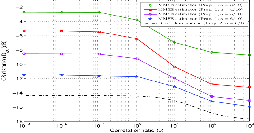
Figure 2: CS distortion $D_{cs}$ (in dB) vs. correlation ratio $\rho$. The parameters are chosen as $N=10$, $K=2$, and $\text{SMNR}_{1}=\text{SMNR}_{2}=10\text{dB}$.

V-B2 End-to-end Distortion

The performance is now tested using the end-to-end MSE, $D$ in (6). It is well-known that VQ is theoretically the optimal block coding strategy, but it suffers in exponential complexity with the dimension of source and bit rate per sample. Therefore, in our simulations, we are compelled to use a low-dimensional setup. All simulations, both in training and in performance evaluation, are performed by using $3\times 10^{5}$ realizations of the source vectors. Further, the vectors $\mathbf{y}_{1}$ and $\mathbf{y}_{2}$ are pre-quantized (as discussed in Section III-D) using $r_{y}=3$ bits per measurement entry in order to obtain $\check{\mathbf{y}}_{1}$ and $\check{\mathbf{y}}_{2}$, respectively.

In our first experiment, we demonstrate the effect of source correlation $\rho$ and measurement rate $\alpha$ on the performance. We use the simulation parameter set ($N=10,K=2,R=R_{1}+R_{2}=10$ bits/vector with $R_{1}=R_{2}$), and assume noiseless communication channels and clean measurements. We vary the correlation ratio from very low $(\rho=10^{-3})$ to very high values $(\rho=10^{3})$, and compare the simulation results with the lower-bound (corresponding to the curve $\alpha=\frac{6}{10}$) derived in (27) of Theorem 1. The results are shown in Figure 3 for various values of measurement rate, i.e., $\alpha=\frac{3}{10},\frac{4}{10},\frac{5}{10},\frac{6}{10}$. From Figure 3, we observe that the higher the correlation (i.e., larger $\rho$) is, the better the performance gets. This behavior was previously observed from the curves in Figure 2 with the objective of CS distortion. As would be expected, at a fixed quantization rate $R$ and correlation ratio $\rho$, increasing $\alpha$ improves the performance, and the curves approach the lower-bound. In this simulation setup, $D_{cs}^{(or)}\ll D_{q}^{(or)}$ (see (27)), hence, the lower-bound mainly shows the contribution of quantization distortion.

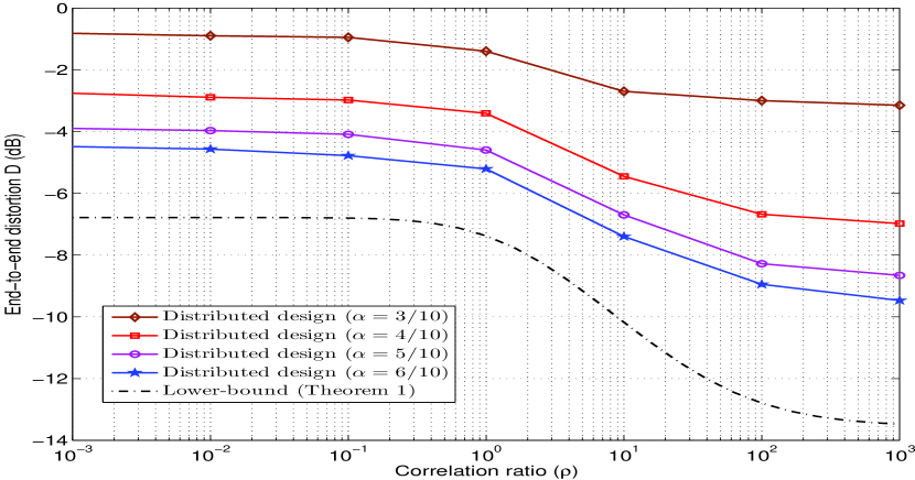
Figure 3: End-to-end distortion ($D$ in dB) vs. correlation ratio $\rho$ using the proposed design scheme along with the lower-bound (27) of Theorem 1 for different values of measurement rate $\alpha$. The parameters are chosen as $N=10$, $K=2$ and $R=R_{1}+R_{2}=10$ bits/vector for clean measurements and noiseless channels.

Next, we investigate how the performance varies by quantization rate. We use the simulation parameter set $(N=10,K=2,M=5,\text{ SMNR}_{1}=\text{SMNR}_{2}=10\text{ dB})$, and assume noiseless communication channels. In Figure 4, we illustrate the end-to-end MSE of the proposed distributed design method as a function of total quantization rate $R=R_{1}+R_{2}$ (with $R_{1}=R_{2}$) for different values of correlation ratios: $\rho=1$ (low-correlated sources), $\rho=10$ (moderately-correlated sources) and $\rho=10^{3}$ (highly-correlated sources). The simulation curves are compared with the lower-bound in (27) corresponding to $\rho=1,10,10^{3}$. From Figure 4, we observe that the performance improves by increasing quantization rate. Moreover, increasing correlation between sources reduces the MSE as observed from the previous experiments too. The gap between the simulation curves and their respective lower-bounds is due to the reason that when CS measurements are noisy, the MMSE estimators $\widetilde{\mathbf{X}}_{l}^{\star}$ $(l\in\{1,2\})$ become far from Gaussian vectors within support. Hence, the simulation curves do not decay as steep as their corresponding lower-bounds which are derived under the optimistic assumption that the source $\mathbf{X}_{l}$ is available for coding. It should be also noted that as quantization rate increases, all the simulation curves will eventually approach to their respective MSE floors, specified by $D_{cs}$. This is reflected from the lower-bounds in Figure 4, where each attains an MSE floor equivalent to $D_{cs}^{(or)}\leq D_{cs}$.

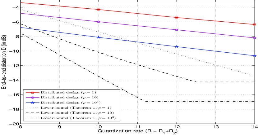
Figure 4: End-to-end distortion ($D$ in dB) vs. quantization rate $R=R_{1}+R_{2}$ (in bits/vector) using the proposed design scheme along with the lower-bound (27) for different values of correlation ratio $\rho$. The parameters are chosen as $N=10$, $K=2$ and $M=5$ for noisy CS measurements, with $\text{SMNR}_{1}=\text{SMNR}_{2}=10$ dB, and noiseless channels.

In our final experiment, we study the impact of channel noise on the performance. In Figure 5, we assess the MSE of the distributed design as a function of channel bit cross-over probability $\epsilon$ (which is the same for channels at both terminals) using the simulation setup $(N=10,K=2,M=5,R=R_{1}+R_{2}=10\text{ bits/vector, with }R_{1}=R_{2})$ and for two values of correlation ratio, $\rho=1,10^{3}$. Further, measurement noise is negligible. In order to demonstrate the efficiency of the distributed design scheme, in Figure 5, we also plot the performance of a centralized design of VQ for CS measurements presented in [40]. A centralized scheme provides benchmark performance where the concatenated measurement vector $\mathbf{Y}=[\mathbf{Y}_{1}^{\top}\hskip 2.84544pt\mathbf{Y}_{1}^{\top}]^{\top}\in\mathbb{R}^{10}$ is encoded using a VQ encoder with $R=10$ bits/vector, and the concatenated source $\mathbf{X}=[\mathbf{X}_{1}^{\top}\hskip 2.84544pt\mathbf{X}_{2}^{\top}]^{\top}\in\mathbb{R}^{20}$ (with $4$ non-zero coefficients) is reconstructed at the decoder. From the simulation curves in Figure 5, it can be observed that degrading channel condition increases MSE. However, the channel-robust VQ design provides robustness against channel noise by considering channel through its design. At high channel noise, the centralized design provides a slightly more robust performance compared to the distributed design, particularly, for the curve corresponding to low correlation. A potential reason is that the centralized design operates on joint source-channel codes of length $10$ bits, while the distributed design has the encoded index of length $5$ bits at each terminal. However, at high correlation ratio, it can be seen that the performance of the distributed design closely follows that of the centralized approach. By comparing the performance of the distributed design at $\rho=1$ and $\rho=10^{3}$, it is revealed that correlation between sources is also useful in providing a better performance in noisy channel scenarios. At very high channel noise level, the performance of the designs for $\rho=1$ and $\rho=10^{3}$ approaches together. To interpret this behavior, let us consider an extreme case where $\epsilon\rightarrow 0.5$. For a BSC with transition probabilities (30), this gives $P(j_{l}|i_{l})\rightarrow\left(1/2\right)^{\mathfrak{R}_{l}}=2^{-2^{R_{l}}},\hskip 7.11317pt\forall i_{l},j_{l},l\in\{1,2\}$, and according to (22), this implies that $P(i_{1},i_{2}|j_{1},j_{2})\rightarrow P(i_{1},i_{2})$, $\forall j_{1},j_{2}$. Studying (21), we get $\textsf{D}_{l}^{\star}(j_{1},j_{2})\rightarrow\mathbb{E}[\mathbf{X}_{l}]$, $\forall j_{l},l\in\{1,2\}$. This means that all the codevectors become equal. Further, studying the expression (19) for the optimized encoding index, we obtain

$$i_{l}^{\star}\!\rightarrow\text{arg }\underset{i_{l}\in\mathcal{I}_{l}}{\text{min }}\left\{\|\mathbb{E}[\mathbf{X}_{l}]\|_{2}^{2}-2\mathbb{E}[\mathbf{X}_{l}^{\top}|\mathbf{y}_{l}]\mathbb{E}[\mathbf{X}_{l}]\right\},\forall j_{l},l\in\{1,2\}.$$

This implies that we have only one non-empty encoding region. Hence, at very high channel noise, only one index is transmitted – irrespective of the input $\mathbf{X}_{l}$ and correlation between sources – and the decoder produces the expected value of the source $\mathbb{E}[\mathbf{X}_{l}]$ for all received indexes from the channel.

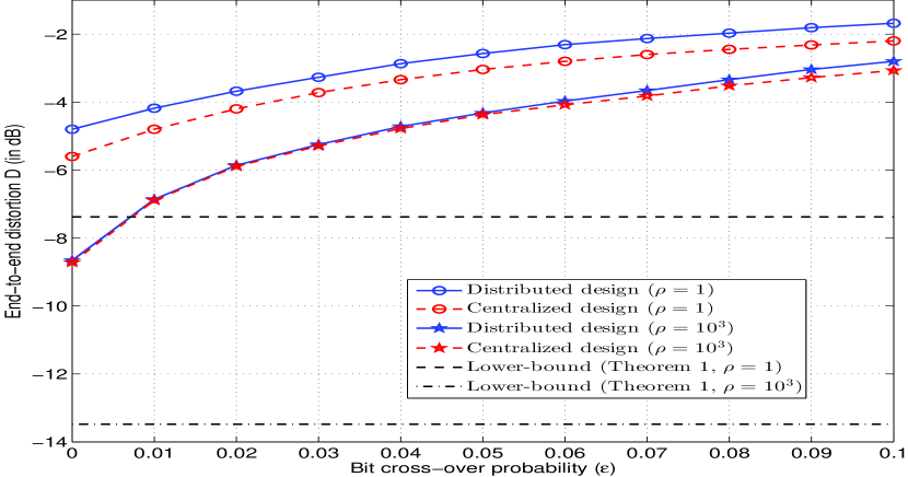
Figure 5: End-to-end MSE ($D$ in dB) vs. channel bit cross-over probability $\epsilon$ using the proposed design scheme along with the lower-bound (27) for different values of correlation ratio $\rho$. The parameters are chosen as $N=10$, $K=2$ and $M=5$ for clean CS measurements, and quantization rate is set to $R=R_{1}+R_{2}=10$ bits/vector, with $R_{1}=R_{2}$.

VI Conclusions and Future Works

We have studied the design and analysis of distributed vector quantization for CS measurements of correlated sparse sources over noisy channels. Necessary conditions for optimality of VQ encoder-decoder pairs have been derived with respect to minimizing end-to-end MSE. We have analyzed the MSE and showed that, without loss of optimality, it is the sum of CS reconstruction MSE and quantized transmission MSE, and we used this fact to derive a lower-bound on the end-to-end MSE. Simulation results have revealed that correlation between sources is an effective factor on the performance in addition to compression resources such as measurement and quantization rates. Further, in noisy channel scenarios, the proposed distributed design method provides robustness against channel noise. In addition, the performance of the distributed design closely follows that of the centralized design.

Finally, we mention that the paper was concerned with full-search VQ schemes suffering from exponential complexity, and hence all experiments were executed with low dimensions. To overcome the complexity issue, a potential future direction is to design sub-optimal structured VQ schemes, such as multistage and tree-structured VQ’s for CS in the distributed setup considered in the paper.

Appendix A Proof of Proposition 1

The MMSE estimator that minimizes $D_{cs}$ in (8) (given noisy CS measurements $\mathbf{y}=[\mathbf{y}_{1}^{\top}\hskip 2.84544pt\mathbf{y}_{2}^{\top}]^{\top}$) is $\widetilde{\mathbf{x}}_{l}^{\star}(\mathbf{y})\triangleq\mathbb{E}[\mathbf{X}_{l}|\mathbf{y}]$ ($l\in\{1,2\}$). Marginalizing over all supports in $\mathbf{\Omega}$, we have

$$\widetilde{\mathbf{x}}_{l}^{\star}(\mathbf{y})=\sum_{\mathcal{S}\subset\mathbf{\Omega}}p(\mathcal{S}|\mathbf{y})\mathbb{E}[\mathbf{X}_{l}|\mathbf{y},\mathcal{S}].$$ (31)

Then, we note the following linear relation

$$\left[\begin{array}[]{c}\mathbf{Y}_{1}\\ \mathbf{Y}_{2}\\ \mathbf{\Theta}_{\mathcal{S}}\\ \mathbf{Z}_{1,\mathcal{S}}\\ \mathbf{Z}_{2,\mathcal{S}}\end{array}\right]=\left[\begin{array}[]{c c c c c}\mathbf{\Phi}_{1,\mathcal{S}}&\mathbf{\Phi}_{1,\mathcal{S}}&\mathbf{0}&\mathbf{I}&\mathbf{0}\\ \mathbf{\Phi}_{2,\mathcal{S}}&\mathbf{0}&\mathbf{\Phi}_{2,\mathcal{S}}&\mathbf{0}&\mathbf{I}\\ \mathbf{I}&\mathbf{0}&\mathbf{0}&\mathbf{0}&\mathbf{0}\\ \mathbf{0}&\mathbf{I}&\mathbf{0}&\mathbf{0}&\mathbf{0}\\ \mathbf{0}&\mathbf{0}&\mathbf{I}&\mathbf{0}&\mathbf{0}\\ \end{array}\right]\cdot\left[\begin{array}[]{c}\mathbf{\Theta}_{\mathcal{S}}\\ \mathbf{Z}_{1,\mathcal{S}}\\ \mathbf{Z}_{2,\mathcal{S}}\\ \mathbf{W}_{1}\\ \mathbf{W}_{2}\end{array}\right],$$ (32)

where for an arbitrary vector or a matrix $\mathbf{A}$, the notation $\mathbf{A}_{\mathcal{S}}$ represents the elements of $\mathbf{A}$ indexed by the support $\mathcal{S}$. Recalling that $\mathbf{\Theta}_{\mathcal{S}}$, $\mathbf{Z}_{l,\mathcal{S}}$ and $\mathbf{W}_{l}$ are all independent Gaussian vectors, the vector on the left-hand-side of (32) is jointly Gaussian. Therefore, based on [45, Theorem 10.2], we have

$$\mathbb{E}\left[[\mathbf{\Theta}_{\mathcal{S}}^{\top}\hskip 2.84544pt\mathbf{Z}_{1,\mathcal{S}}^{\top}\hskip 2.84544pt\mathbf{Z}_{2,\mathcal{S}}^{\top}]^{\top}\hskip 2.84544pt\big{|}\mathbf{y}\right]=\mathbf{C}^{\top}\mathbf{D}^{-1}\mathbf{y},$$ (33)

where $\mathbf{C}$ and $\mathbf{D}$ are covariance matrices specified in (11d) and (11g), respectively. Now, since $\mathbb{E}[\mathbf{X}_{l,\mathcal{S}}|\mathbf{y}]=\mathbb{E}[\mathbf{\Theta}_{\mathcal{S}}|\mathbf{y}]+\mathbb{E}[\mathbf{Z}_{l,\mathcal{S}}|\mathbf{y}]$ ($l\in\{1,2\}$), it follows that within support set $\mathcal{S}$, we obtain

$$\widetilde{\mathbf{x}}^{\star}(\mathbf{y},\mathcal{S})\triangleq\left[\begin{array}[]{c}\widetilde{\mathbf{x}}_{1}^{\star}(\mathbf{y},\mathcal{S})\\ \widetilde{\mathbf{x}}_{2}^{\star}(\mathbf{y},\mathcal{S})\\ \end{array}\right]=\left[\begin{array}[]{c c c}\mathbf{I}&\mathbf{I}&\mathbf{0}\\ \mathbf{I}&\mathbf{0}&\mathbf{I}\\ \end{array}\right]\mathbf{C}^{\top}\mathbf{D}^{-1}\mathbf{y},$$ (34)

and otherwise zero.

Now, it only remains to find an expression for $p(\mathcal{S}|\mathbf{y})$ in (31). Let us first define $\mathbf{q}_{\mathcal{S}}\triangleq[\mathbf{\theta}_{\mathcal{S}}^{\top}\hskip 2.84544pt\mathbf{z}_{1,\mathcal{S}}^{\top}\hskip 2.84544pt\mathbf{z}_{2,\mathcal{S}}^{\top}]^{\top}$, then

$$p(\mathcal{S}|\mathbf{y}) =\frac{p(\mathbf{y}|\mathcal{S})p(\mathcal{S})}{\sum_{\mathcal{S}}p(\mathbf{y}|\mathcal{S})p(\mathcal{S})}$$ (35)

$$=\frac{\int_{\mathbf{q}_{\mathcal{S}}}p(\mathbf{q}_{\mathcal{S}}|\mathcal{S})p(\mathbf{y}|\mathbf{q}_{\mathcal{S}},\mathcal{S})d\mathbf{q}_{\mathcal{S}}}{\sum_{\mathcal{S}}\int_{\mathbf{q}_{\mathcal{S}}}p(\mathbf{q}_{\mathcal{S}}|\mathcal{S})p(\mathbf{y}|\mathbf{q}_{\mathcal{S}},\mathcal{S})d\mathbf{q}_{\mathcal{S}}},$$

where we used the fact that $p(\mathcal{S})=\frac{1}{{N\choose K}}$. It can be verified that $p(\mathbf{q}_{\mathcal{S}}|\mathcal{S})=\mathcal{N}(\mathbf{0},\mathbf{E})$ and $p(\mathbf{y}|\mathbf{q}_{\mathcal{S}},\mathcal{S})=\mathcal{N}(\mathbf{Fq}_{\mathcal{S}},\mathbf{N})$, where the matrices $\mathbf{N}$, $\mathbf{E}$ and $\mathbf{F}$ are specified in (11j), (11n) and (11q), respectively. Therefore, it follows that

$$p(\mathbf{q}_{\mathcal{S}}|\mathcal{S}) =\frac{1}{\sqrt{(2\pi)^{3K}\det(\mathbf{E})}}e^{-\frac{1}{2}\mathbf{q}_{\mathcal{S}}^{\top}\mathbf{E}^{-1}\mathbf{q}_{\mathcal{S}}}$$ (36)

$$p(\mathbf{y}|\mathbf{q}_{\mathcal{S}},\mathcal{S}) =\frac{1}{\sqrt{(2\pi)^{2M}\det(\mathbf{N})}}e^{-\frac{1}{2}(\mathbf{y}-\mathbf{Fq}_{\mathcal{S}})^{\top}\mathbf{N}^{-1}(\mathbf{y}-\mathbf{Fq}_{\mathcal{S}})}.$$

Using the Gaussian distributions in (36), we get

$$p(\mathbf{q}_{\mathcal{S}}|\mathcal{S})p(\mathbf{y}|\mathbf{q}_{\mathcal{S}},\mathcal{S}) \!=\!\frac{e^{-\mathbf{y}^{\top}\mathbf{N}^{-\!1}\mathbf{y}}}{\sqrt{(2\pi)^{3K+\!2M}\det(\mathbf{E})\det(\mathbf{N})}}$$ (37)

$$\times e^{-\frac{1}{2}\left(\mathbf{q}_{\mathcal{S}}^{\top}\left(\mathbf{E}^{-\!1}\!+\!\mathbf{F}^{\top}\mathbf{N}^{-\!1}\mathbf{F}\right)\mathbf{q}_{\mathcal{S}}\!-\!2\mathbf{y}^{\top}\mathbf{N}^{-\!1}\mathbf{F}\mathbf{q}_{\mathcal{S}}\right)}.$$

Now, using [46, eq. (346)], it yields

$$\int_{\mathbf{q}_{\mathcal{S}}}p(\mathbf{q}_{\mathcal{S}}|\mathcal{S})p(\mathbf{y}|\mathbf{q}_{\mathcal{S}},\mathcal{S})d\mathbf{q}_{\mathcal{S}}=$$ (38)

$$\hskip 17.07182pt\frac{e^{\frac{1}{2}\mathbf{y}^{\top}\left(\mathbf{N}^{-1}\mathbf{F}^{\top}\left(\mathbf{E}^{-1}+\mathbf{F}^{\top}\mathbf{N}^{-1}\mathbf{F}\right)^{-1}\mathbf{F}\mathbf{N}^{-1}-\mathbf{N}^{-1}\right)\mathbf{y}}}{\sqrt{(2\pi)^{2M-3K}\det(\mathbf{N})\det(\mathbf{E}^{-1}+\mathbf{F}^{\top}\mathbf{N}^{-1}\mathbf{F})}}.$$

Plugging (38) back into (35) yields $\beta_{\mathcal{S}}$ in (11a), and the proof is concluded. $\hfill\blacksquare$

Appendix B Proof of Proposition 2

The oracle estimator is obtained by (10) given $\mathcal{S}^{(or)}$. Then, it follows from the law of total expectation that

$$D_{cs}^{(or)}=\frac{1}{2K}\mathbb{E}\left[\sum_{l=1}^{2}\mathbb{E}\left[\|\mathbf{X}_{l,\mathcal{S}^{(or)}}-\widetilde{\mathbf{X}}_{l,\mathcal{S}^{(or)}}\|_{2}^{2}\right]\right],$$ (39)

where the inner expectation is taken over the distribution of $\mathbf{X}_{l}$ given the oracle-known support, and the outer expectation is taken over all possibilities of oracle support set. Further, $\widetilde{\mathbf{X}}_{l,\mathcal{S}^{(or)}}\triangleq\mathbb{E}[\mathbf{X}_{l,\mathcal{S}^{(or)}}|\mathbf{Y}]\in\mathbb{R}^{K}$, $l\in\{1,2\}$.

Defining $\mathbf{Q}_{\mathcal{S}}\triangleq[\mathbf{\Theta}_{\mathcal{S}}^{\top}\hskip 2.84544pt\mathbf{Z}_{1,\mathcal{S}}^{\top}\hskip 2.84544pt\mathbf{Z}_{2,\mathcal{S}}^{\top}]^{\top}$, for $l\!=\!1$, we have

$$\mathbb{E}\left[\left(\mathbf{X}_{1,\mathcal{S}^{(or)}}-\widetilde{\mathbf{X}}_{1,\mathcal{S}^{(or)}}\right)\left(\mathbf{X}_{1,\mathcal{S}^{(or)}}-\widetilde{\mathbf{X}}_{1,\mathcal{S}^{(or)}}\right)^{\top}\right]$$ (40)

$$\!\stackrel{{\scriptstyle(a)}}{{=}}\left[\mathbf{I}\hskip 4.26773pt\mathbf{I}\hskip 4.26773pt\mathbf{0}\right]\mathbb{E}\left[\left(\mathbf{Q}_{\mathcal{S}^{(or)}}\!-\!\widetilde{\mathbf{Q}}_{\mathcal{S}^{(or)}}\right)\left(\mathbf{Q}_{\mathcal{S}^{(or)}}\!-\!\widetilde{\mathbf{Q}}_{\mathcal{S}^{(or)}}\right)^{\!\top}\right]\left[\mathbf{I}\hskip 4.26773pt\mathbf{I}\hskip 4.26773pt\mathbf{0}\right]^{\top}$$

$$\!\stackrel{{\scriptstyle(b)}}{{=}}\left[\mathbf{I}\hskip 4.26773pt\mathbf{I}\hskip 4.26773pt\mathbf{0}\right]\left(\mathbf{E}-\mathbf{C}^{\top}\mathbf{D}^{-1}\mathbf{C}\right)\left[\mathbf{I}\hskip 4.26773pt\mathbf{I}\hskip 4.26773pt\mathbf{0}\right]^{\top},$$

where $(a)$ follows from the fact that $\mathbf{X}_{1,\mathcal{S}}=\left[\mathbf{I}\hskip 4.26773pt\mathbf{I}\hskip 4.26773pt\mathbf{0}\right]\mathbf{Q}_{\mathcal{S}}$, and $(b)$ can be shown from [45, Theorem 10.2]. Similarly, for $l=2$, we obtain

$$\mathbb{E}\left[\left(\mathbf{X}_{2,\mathcal{S}^{(or)}}-\widetilde{\mathbf{X}}_{2,\mathcal{S}^{(or)}}\right)\left(\mathbf{X}_{2,\mathcal{S}^{(or)}}-\widetilde{\mathbf{X}}_{2,\mathcal{S}^{(or)}}\right)^{\top}\right]$$ (41)

$$=\left[\mathbf{I}\hskip 4.26773pt\mathbf{0}\hskip 4.26773pt\mathbf{I}\right]\left(\mathbf{E}-\mathbf{C}^{\top}\mathbf{D}^{-1}\mathbf{C}\right)\left[\mathbf{I}\hskip 4.26773pt\mathbf{0}\hskip 4.26773pt\mathbf{I}\right]^{\top}.$$

Combining (40) and (41) with (39), it follows that

$$D_{cs}^{(or)} \stackrel{{\scriptstyle(a)}}{{=}}\frac{1}{2K}\mathbb{E}\left[\text{Tr}\left\{\left[\begin{array}[]{c c c}2\mathbf{I}&\mathbf{I}&\mathbf{I}\\ \mathbf{I}&\mathbf{I}&\mathbf{0}\\ \mathbf{I}&\mathbf{I}&\mathbf{I}\\ \end{array}\right]\left(\mathbf{E}-\mathbf{C}^{\top}\mathbf{D}^{-1}\mathbf{C}\right)\right\}\right]$$ (42)

$$\stackrel{{\scriptstyle(b)}}{{=}}\!1\!-\!\frac{1}{2K}\left[\text{Tr}\left\{\left[\begin{array}[]{c c c}2\mathbf{I}&\mathbf{I}&\mathbf{I}\\ \mathbf{I}&\mathbf{I}&\mathbf{0}\\ \mathbf{I}&\mathbf{I}&\mathbf{I}\\ \end{array}\right]\frac{1}{{N\choose K}}\sum_{\mathcal{S}^{(or)}}\mathbf{C}^{\!\top}\mathbf{D}^{-\!1}\mathbf{C}\right\}\right]$$

where $(a)$ follows from fact that for two matrices $\mathbf{A}$ and $\mathbf{B}$ with appropriate dimensions, we have $\text{Tr}\{\mathbf{A+B}\}=\text{Tr}\{\mathbf{A}\}+\text{Tr}\{\mathbf{B}\}$ and $\text{Tr}\{\mathbf{AB}\}=\text{Tr}\{\mathbf{BA}\}$. Also, $(b)$ follows the uniform distribution of a possible oracle-known support set, and simple matrix algebra. $\hfill\blacksquare$

Appendix C Proof of Proposition 3

The proof follows the same line of arguments in the proof of Proposition 1. Let $\mathbf{q}_{\mathcal{S}}\triangleq[\mathbf{\theta_{s}}^{\top}\hskip 2.84544pt\mathbf{z}_{1,\mathcal{S}}^{\top}\hskip 2.84544pt\mathbf{z}_{2,\mathcal{S}}^{\top}]^{\top}$ and $\mathbf{g}_{\mathcal{S}}\triangleq[\mathbf{\theta_{s}}^{\top}\hskip 2.84544pt\mathbf{z}_{1,\mathcal{S}}^{\top}]^{\top}$, then we rewrite $p(\mathbf{y}_{2}|\mathbf{y}_{1})$ as

$$p(\mathbf{y}_{2}|\mathbf{y}_{1}) =\frac{\sum_{\mathcal{S}}p(\mathbf{y}_{1},\mathbf{y}_{2}|\mathcal{S})P(\mathcal{S})}{\sum_{\mathcal{S}}p(\mathbf{y}_{1}|\mathcal{S})P(\mathcal{S})}$$ (43)

$$=\frac{\sum_{\mathcal{S}}\int_{\mathbf{q}_{\mathcal{S}}}p(\mathbf{q}_{\mathcal{S}}|\mathcal{S})p(\mathbf{y}_{1},\mathbf{y}_{2}|\mathbf{q}_{\mathcal{S}},\mathcal{S})d\mathbf{q}_{\mathcal{S}}}{\sum_{\mathcal{S}}\int_{\mathbf{g}_{\mathcal{S}}}p(\mathbf{g}_{\mathcal{S}}|\mathcal{S})p(\mathbf{y}_{1}|\mathbf{g}_{\mathcal{S}},\mathcal{S})d\mathbf{g}_{\mathcal{S}}}.$$

It was shown in the proof of Proposition 1 that $p(\mathbf{q}_{\mathcal{S}}|\mathcal{S})$ and $p(\mathbf{y}_{1},\mathbf{y}_{2}|\mathbf{q}_{\mathcal{S}},\mathcal{S})$ are Gaussian pdf’s with known mean vectors and covariance matrices. Further, it can be easily shown that $p(\mathbf{g}_{\mathcal{S}}|\mathcal{S})=\mathcal{N}(\mathbf{0},\text{bdiag}(\sigma_{\theta}^{2}\mathbf{I},\sigma_{z}^{2}\mathbf{I}))$, where $\text{bdiag}(\cdot)$ denotes the block diagonal matrix with diagonal matrices $\sigma_{\theta}^{2}\mathbf{I}$ and $\sigma_{z}^{2}\mathbf{I}$ as its blocks. Also, $p(\mathbf{y}_{1}|\mathbf{g}_{\mathcal{S}},\mathcal{S})=\mathcal{N}(\mathbf{\Psi}\mathbf{g}_{\mathcal{S}},\sigma_{w_{1}}^{2}\mathbf{I})$, where $\mathbf{\Psi}\triangleq[\mathbf{\Phi}_{1,\mathcal{S}}\hskip 4.26773pt\mathbf{\Phi}_{1,\mathcal{S}}]$. The integrations in the numerator and denominator of the last equation in (43) can be analytically derived, similar to the ones in the proof of Proposition 1, leading to the expression in (14). $\hfill\blacksquare$

Appendix D Proof of Theorem 1

We start with the decomposition of the end-to-end MSE in (26) as $D=D_{cs}+D_{q}$. Finding expressions for $D_{q}$ is non-trivial due to lack of analytical tractability and unknown probability distribution of sparse sources, and their MMSE reconstructions. Alternatively, we introduce two lower-bounds to $D$. The first relation is

$$D>D_{cs}\geq D_{cs}^{(or)}.$$ (44)

Next, we note that the performance of the studied system is always poorer than that of a system where $\mathbf{X}_{1}$ and $\mathbf{X}_{2}$ are available for coding directly (with oracle known support set $\mathcal{S}^{(or)}$). Hence, we have

$$D\geq\frac{1}{2K}\sum_{l=1}^{2}\mathbb{E}[\|\mathbf{X}_{l}|_{\mathcal{S}^{(or)}}-\widehat{\mathbf{X}}_{l}|_{\mathcal{S}^{(or)}}\|_{2}^{2}],$$ (45)

where we denote by $\mathbf{X}_{l}|_{\mathcal{S}^{(or)}}\in\mathbb{R}^{N}$ the source $\mathbf{X}_{l}$ with oracle known support set $\mathcal{S}^{(or)}$, and $\widehat{\mathbf{X}}_{l}|_{\mathcal{S}^{(or)}}\in\mathbb{R}^{N}$ denotes decoded vector with known support. Since elements of support set are iid and uniformly drawn from all possibilities, a natural approach is to allocate $R_{0}=\log_{2}{N\choose K}$ bits to transmit $\mathcal{S}^{(or)}$ which is received without loss. Then, we only need to find the distortion-rate function for two correlated Gaussian sources using $R_{1}+R_{2}-\log_{2}{N\choose K}$. Let us denote the non-sparse correlated Gaussian sources by $\mathbf{X}_{1,\mathcal{S}},\mathbf{X}_{2,\mathcal{S}}\in\mathbb{R}^{K}$. The rate region for the quadratic Gaussian problem of two-terminal source coding has been developed in [12] so that we can lower-bound the last expression in (45). For this purpose, let us define $D_{l,\mathcal{S}^{(or)}}\triangleq\frac{1}{K}\mathbb{E}[\|\mathbf{X}_{l,\mathcal{S}^{(or)}}-\widehat{\mathbf{X}}_{l,\mathcal{S}^{(or)}}\|_{2}^{2}]$, $l\in\{1,2\}$, then with some mathematical simplifications of the results in [12, Theorem 1], we obtain

$$D_{1,\mathcal{S}^{(or)}}D_{2,\mathcal{S}^{(or)}} \geq\left(1\!-\!\frac{\rho^{2}}{(1-\rho)^{2}}\right)2^{\frac{-2\left(R_{1}+R_{2}-\log_{2}{N\choose K}\right)}{K}}$$ (46)

$$+\frac{\rho^{2}}{(1-\rho)^{2}}2^{\frac{-4\left(R_{1}+R_{2}-\log_{2}{N\choose K}\right)}{K}}.$$

Since $D_{1,\mathcal{S}^{(or)}}$ is inversely proportional to $D_{2,\mathcal{S}^{(or)}}$, then $\frac{1}{2K}\sum_{l=1}^{2}D_{l,\mathcal{S}^{(or)}}$ is minimized by setting $D_{1,\mathcal{S}^{(or)}}=D_{2,\mathcal{S}^{(or)}}$. Combining this fact with (46) and (45), it follows that

$$D \geq\left(\left(1\!-\!\frac{\rho^{2}}{(1-\rho)^{2}}\right)2^{\frac{-2\left(R_{1}+R_{2}-\log_{2}{N\choose K}\right)}{K}}\right.$$ (47)

$$\left.+\frac{\rho^{2}}{(1-\rho)^{2}}2^{\frac{-4\left(R_{1}+R_{2}-\log_{2}{N\choose K}\right)}{K}}\right)^{\frac{1}{2}}\triangleq D_{q}^{(or)}.$$

From the lower-bounds (44) and (47), it can be inferred that the former is tighter when CS measurements are noisy, and the latter is tighter when there is no loss due to CS distortion. Therefore, in order to adaptively consider both regimes, we develop a composite lower-bound by combining them as

$$D>\max\left\{D_{cs}^{(or)},D_{q}^{(or)}\right\},$$ (48)

which concludes the proof.

It can be also seen from (27) that the channel aspects are not considered in developing the lower-bound. This is due to fact that the source-channel separation theorem is not optimal in the case of our studied distributed system, therefore, the minimum MSE (in terms of distortion-rate function over a DMC) cannot be analytically derived (based on channel capacity) in the scenario of noisy channels. As a result, when channel becomes very noisy, the lower-bound is not theoretically attainable. $\hfill\blacksquare$

References

- [1] R. Gray and D. Neuhoff, “Quantization,” IEEE Trans. Inf. Theory, vol. 44, no. 6, pp. 2325–2383, October 1998.
- [2] E. Candes and M. Wakin, “An introduction to compressive sampling,” IEEE Sig. Proc. Magazine, vol. 25, no. 2, pp. 21 –30, Mar. 2008.
- [3] T. Lookabaugh and R. Gray, “High-resolution quantization theory and the vector quantizer advantage,” IEEE Trans. Inf. Theory, vol. 35, no. 5, pp. 1020–1033, September 1989.
- [4] D. Slepian and J. Wolf, “Noiseless coding of correlated information sources,” IEEE Trans. Inf. Theory, vol. 19, no. 4, pp. 471–480, 1973.
- [5] A. Wyner and J. Ziv, “The rate-distortion function for source coding with side information at the decoder,” IEEE Trans. Inf. Theory, vol. 22, no. 1, pp. 1–10, 1976.
- [6] R. Zamir and T. Berger, “Multiterminal source coding with high resolution,” IEEE Trans. Inf. Theory, vol. 45, no. 1, pp. 106–117, 1999.
- [7] Z. Xiong, A. Liveris, and S. Cheng, “Distributed source coding for sensor networks,” IEEE Sig. Proc. Magazine, vol. 21, no. 5, pp. 80–94, 2004.
- [8] J. Chen, X. Zhang, T. Berger, and S. Wicker, “An upper bound on the sum-rate distortion function and its corresponding rate allocation schemes for the CEO problem,” IEEE Journal on Select. Areas in Commun., vol. 22, no. 6, pp. 977–987, 2004.
- [9] Y. Oohama, “Rate-distortion theory for Gaussian multiterminal source coding systems with several side informations at the decoder,” IEEE Trans. Inf. Theory, vol. 51, no. 7, pp. 2577–2593, 2005.
- [10] M. Gastpar, P. L. Dragotti, and M. Vetterli, “The distributed Karhunen-Loève transform,” IEEE Trans. Inf. Theory, vol. 52, no. 12, pp. 5177–5196, 2006.
- [11] D. Rebollo-Monedero, S. Rane, A. Aaron, and B. Girod, “High-rate quantization and transform coding with side information at the decoder,” Signal Processing, vol. 86, no. 11, pp. 3160 – 3179, 2006.
- [12] A. Wagner, S. Tavildar, and P. Viswanath, “Rate region of the quadratic Gaussian two-encoder source-coding problem,” IEEE Trans. Inf. Theory, vol. 54, no. 5, pp. 1938–1961, 2008.
- [13] P. L. Dragotti and M. Gastpar, Distributed Source Coding: Theory, Algorithms and Applications. Academic Press, 2009.
- [14] N. Wernersson, J. Karlsson, and M. Skoglund, “Distributed quantization over noisy channels,” IEEE Trans. Commun., vol. 57, no. 6, pp. 1693–1700, 2009.
- [15] N. Wernersson and M. Skoglund, “Nonlinear coding and estimation for correlated data in wireless sensor networks,” IEEE Trans. Commun., vol. 57, no. 10, pp. 2932–2939, 2009.
- [16] J. Sun, V. Misra, and V. Goyal, “Distributed functional scalar quantization simplified,” IEEE Trans. Sig. Proc., vol. 61, no. 14, pp. 3495–3508, 2013.
- [17] X. Chen and E. Tuncel, “Zero-delay joint source-channel coding using hybrid digital-analog schemes in the Wyner-Ziv setting,” IEEE Trans. Commun., vol. 62, no. 2, pp. 726–735, February 2014.
- [18] E. Candes, J. Romberg, and T. Tao, “Stable signal recovery from incomplete and inaccurate measurements,” Comm. Pure Appl. Math, vol. 59, no. 8, pp. 1207–1223, 2006.
- [19] C. Güntürk, M. Lammers, A. Powell, R. Saab, and O. Ylmaz, “Sigma delta quantization for compressed sensing,” in Annual Conf. Inf. Sciences and Systems, March 2010, pp. 1 –6.
- [20] A. Zymnis, S. Boyd, and E. Candes, “Compressed sensing with quantized measurements,” IEEE Sig. Proc. Lett., vol. 17, no. 2, pp. 149 –152, Feb. 2010.
- [21] W. Dai and O. Milenkovic, “Information theoretical and algorithmic approaches to quantized compressive sensing,” IEEE Trans. Commun., vol. 59, no. 7, pp. 1857 –1866, Jul. 2011.
- [22] L. Jacques, D. Hammond, and J. Fadili, “Dequantizing compressed sensing: When oversampling and non-Gaussian constraints combine,” IEEE Trans. Inf. Theory, vol. 57, no. 1, pp. 559 –571, Jan. 2011.
- [23] M. Yan, Y. Yang, and S. Osher, “Robust 1-bit compressive sensing using adaptive outlier pursuit,” IEEE Trans. Sig. Proc., vol. 60, no. 7, pp. 3868 –3875, Jul. 2012.
- [24] U. S. Kamilov, V. K. Goyal, and S. Rangan, “Message-passing de-quantization with applications to compressed sensing,” IEEE Trans. Sig. Proc., vol. 60, no. 12, pp. 6270 –6281, Dec. 2012.
- [25] J. Sun and V. Goyal, “Optimal quantization of random measurements in compressed sensing,” in IEEE Int. Symp. Inf. Theory, Jul. 2009, pp. 6 –10.
- [26] P. Boufounos, “Universal rate-efficient scalar quantization,” IEEE Trans. Inf. Theory, vol. 58, no. 3, pp. 1861 –1872, March 2012.
- [27] U. Kamilov, V. Goyal, and S. Rangan, “Optimal quantization for compressive sensing under message passing reconstruction,” in IEEE Int. Symp. Inf. Theory, 31 2011-Aug. 5 2011, pp. 459 –463.
- [28] A. Shirazinia, S. Chatterjee, and M. Skoglund, “Performance bounds for vector quantized compressive sensing,” in Int. Symp. Inf. Theory and App., Oct. 2012, pp. 289 –293.
- [29] ——, “Analysis-by-synthesis quantization for compressed sensing measurements,” IEEE Trans. Sig. Proc., vol. 61, no. 22, pp. 5789–5800, 2013.
- [30] V. Goyal, A. Fletcher, and S. Rangan, “Compressive sampling and lossy compression,” IEEE Sig. Proc. Mag., vol. 25, no. 2, pp. 48–56, March 2008.
- [31] J. Laska and R. Baraniuk, “Regime change: Bit-depth versus measurement-rate in compressive sensing,” IEEE Trans. Sig. Proc., vol. 60, no. 7, pp. 3496 –3505, Jul. 2012.
- [32] W. Bajwa, J. Haupt, A. Sayeed, and R. Nowak, “Joint source-channel communication for distributed estimation in sensor networks,” IEEE Trans. Inf. Theory, vol. 53, no. 10, pp. 3629–3653, 2007.
- [33] D. Baron, M. F. Duarte, M. B. Wakin, S. Sarvotham, and R. G. Baraniuk, “Distributed compressive sensing,” CoRR, vol. abs/0901.3403, 2009.
- [34] M. Rambeloarison, S. Feizi, G. Angelopoulos, and M. Medard, “Empirical rate-distortion study of compressive sensing-based joint source-channel coding,” in Asilomar Conference Sig., Systems and Computers, 2012, pp. 1224–1228.
- [35] S. Feizi, M. Medard, and M. Effros, “Compressive sensing over networks,” in Allerton Conf. Commun., Control and Computing, 2010, pp. 1129–1136.
- [36] M. Nabaee and F. Labeau, “Quantized network coding for correlated sources,” CoRR, vol. abs/1212.5288, 2012.
- [37] S. Cheng, V. Stankovic, and L. Stankovic, “An efficient spectrum sensing scheme for cognitive radio,” IEEE Sig. Proc. Lett., vol. 16, no. 6, pp. 501–504, June 2009.
- [38] A. Gilbert and J. Tropp, “Applications of sparse approximation in communications,” in IEEE Int. Symp. Inf. Theory, 2005, pp. 1000–1004.
- [39] J. Tropp, A. Gilbert, and M. Strauss, “Simultaneous sparse approximation via greedy pursuit,” in IEEE Int. Conf. Acoust. Speech, and Sig. Proc., vol. 5, 2005, pp. 721–724.
- [40] A. Shirazinia, S. Chatterjee, and M. Skoglund, “Channel-optimized vector quantizer design for compressed sensing measurements,” in IEEE Int. Conf. Acoust. Speech, and Sig. Proc., 2013, pp. 4648–4652.
- [41] A. Gersho and R. M. Gray, Vector Quantization and Signal Compression. Kluwer Academic Publishers, 1991.
- [42] Y. Linde, A. Buzo, and R. Gray, “An algorithm for vector quantizer design,” IEEE Trans. Commun., vol. 28, no. 1, pp. 84 – 95, Jan 1980.
- [43] N. Phamdo, N. Farvardin, and T. Moriya, “A unified approach to tree-structured and multistage vector quantization for noisy channels,” IEEE Trans. Inf. Theory, vol. 39, no. 3, pp. 835 –850, May 1993.
- [44] M. Duarte and Y. Eldar, “Structured compressed sensing: From theory to applications,” IEEE Trans. Sig. Proc., vol. 59, no. 9, pp. 4053–4085, September 2011.
- [45] S. Kay, Fundamentals of Statistical Signal Processing: Estimation Theory. Englewood Cliffs, NJ: Prentice Hall, 1993.
- [46] K. B. Petersen and M. S. Pedersen, “The matrix cookbook,” nov 2012, version 20121115. [Online]. Available: http://www2.imm.dtu.dk/pubdb/p.php?3274