Testing for shielding of special nuclear weapon materials

Abstract

Nuclear-weapon-material detection via gamma-ray sensing is routinely applied, for example, in monitoring cross-border traffic. Natural or deliberate shielding both attenuates and distorts the shape of the gamma-ray spectra of specific radionuclides, thereby making such routine applications challenging. We develop a Lagrange multiplier (LM) test for shielding. A strong advantage of the LM test is that it only requires fitting a much simpler model that assumes no shielding. We show that, under the null hypothesis and some mild regularity conditions and as the detection time increases, LM test statistic for (composite) shielding is asymptotically Chi-square with the degree of freedom equal to the presumed number of shielding materials. We also derive the local power of the LM test. Extensive simulation studies suggest that the test is robust to the number and nature of the intervening materials, which owes to the fact that common intervening materials have broadly similar attenuation functions.

, , and t1Supported in part by Department of Energy, DE-FG52-09NA29364, PDP08-028.

1 Introduction

A major homeland security issue concerns monitoring cross-border traffic to prevent terrorists from smuggling nuclear weapon materials into the US [Medalia (2009)]. This requires screening cargoes which may contain illegal radioactive materials, for example, special nuclear weapon materials (SNWM). A radioactive material generally gives off alpha, beta and gamma emissions, and some material also gives off neutrons. Gamma ray spectra are often used to detect specific nuclear materials, due to their unique signature and the fact that gamma rays can travel relatively long distances through most objects. Active detection methods [Fetter et al. (1990), Moss et al. (2002)] can detect quite small amounts of radioactive material, but they are generally not preferable because they can be destructive and harmful to humans. Consequently, passive sensing [August and Whitlock (2005)] is the prime detection approach.

In many applications (e.g., cargo screening), gamma-ray signature recognition is plagued by the problem of weak signals, owing to (i) relatively large distances between the radioactive source and the detector (spectrometer) and (ii) natural or deliberate shielding by intervening materials. Furthermore, primary screening uses very low resolution detectors, and higher resolution NaI detectors are used almost exclusively in secondary vehicle screening when an alert is generated in primary screening. Shielding not only attenuates the signal but it also distorts the overall shape of the gamma ray spectrum, as the strength of attenuation is specific to the energy (level) of the gamma ray and increases exponentially with the thickness of the intervening material. Since the nature and the thickness of the shielding materials are generally unknown, shielding makes the problem of nuclide detection via gamma-ray signature recognition challenging.

In the case of strong unshielded sources or long averaging times, radionuclide detection can be carried out by peak finding methods [Jarman et al. (2003)] and the library least-squares approach (LLS) [Marshall and Zumberge (1989), Gardner and Xu (2009)]. The latter approach is based on the principle that the pulse height (gamma ray) spectrum recorded by a detector (the photon counts as a function of photon energy) is, on average, equal to the weighted sum of the detector response functions (DRF) to the gamma rays reaching the detector, plus that of the background radiation, where the weights are the intensities of the gamma rays. Consequently, the problem of deducing which radionuclides are in the source may, in principle, be reduced to a regression problem. Assuming no shielding, the relative intensities of the gamma rays emitted by a radionuclide of interest are known so that their detector response functions can be combined into one single detector response function unique to the radionuclide, which makes the regression problem more manageable.

In the general case of shielding, all gamma rays emitted by radionuclides of interest and all the ways in which they may be attenuated or modified must be included in the regression model. Their DRFs may be modeled semiparametrically [Mitchell, Sanger and Marlow (1989)] or by Monte Carlo techniques as used in the Monte Carlo N-Particle code (MCNP) [Cashwell, Everett and Rechard (1957)] and GEometry ANd Tracking (GEANT) [Allison et al. (2006)]. The library of all relevant DRFs is then quite large, introducing multicollinearity and increasing the number of parameters, which renders this approach not practical. This problem can be solved by (i) grouping the detector response functions nuclide by nuclide, (ii) noting that the coefficients are all positive for a group if the corresponding nuclide is present, and (iii) recognizing that only a few radionuclides may be present in the source so that the regression model is sparse, that is, most of the regression coefficients are zero; see Chan et al. (2012), Bai et al. (2011) and Kump et al. (2012).

In principle, gamma ray recognition may be enhanced by incorporating the physical laws of shielding. However, given the unknown nature of the shielding material(s) of unknown thickness, a model-based approach would require estimating a rather complex and nonlinearly parameterized model. Here, we develop a Lagrange multiplier (LM) test for shielding by known intervening materials which only requires fitting the much simpler model under the null hypothesis of no shielding. Our approach assumes that the mean background radiation (due to naturally occurring radioactive sources, e.g., cosmic rays, granite, etc.) is known and we are interested in detecting the presence of specific radionuclides, a relatively easy task, in the absence of shielding. Thus, the critical problem is to test for the presence of shielding, under the framework of screening for specific radionuclides embedded in background radiation. Solving this problem is pertinent to achieving the real goal of detecting the known sources, as detecting shielding would trigger human inspection. We show that the LM test statistic has an asymptotic Chi-square distribution under the null hypothesis of no shielding, with the degree of freedom equal to the presumed number of shielding materials. The attenuation patterns of commonly used intervening materials (e.g., carbon, lead, concrete and water) are broadly similar. It turns out that this broad similarity results in the pleasant surprising consequence that the power of the LM test appears to be robust to the nature and number of common intervening materials, as suggested by our simulation results.

The paper is organized as follows. In Section 2 we introduce the model for the pulse height spectrum under shielding. In Section 3 we derive the Lagrange multiplier test and its asymptotic null distribution. The asymptotic power of the test is obtained in Section 4. Extensive simulations with shielding by simple or composite intervening materials are reported in Section 5. Our approach focuses on attenuation of the gamma rays by intervening materials but ignores the secondary effects of down scattering of the gamma-ray spectra due to Compton scattering of the gamma rays outside the detector, which introduces errors in the DRFs by changing the relative contributions of each of the emissions from the radionuclide and by changing the shape and intensity of the background radiation. Indeed, background radiation generally varies over time, for example, it is subject to vehicle suppression in cargo screening [Lo Presti et al. (2006)]. See Burr and Hamada (2009) for a review on the difficulties and challenges of isotope identification using fielded NaI detectors. Furthermore, DRF is detector-specific and may be unstable over time. In Section 6 we perform a sensitivity analysis of the proposed method against errors in the DRFs and the background radiation. We conclude in Section 7 by pointing out some future research necessary before field deployment of the proposed methods.

It is desirable to test the proposed method with real data. However, to access real data from any US port of entry, red tape has to be overcome and the process has proved to be much harder than expected due to potential national security issues. The data used in the paper are semi-real in the sense that the background was based on a real background and isotope spectra were synthetically superimposed on the background according to the standard and data published by the National Institute of Standards and Technology (NIST).

2 A Poisson regression model for shielding

Before presenting the statistical model for shielding, we outline the physics underlying shielding of radionuclides; see Bryan (2008), Maher and Wikibooks Contributors (2008), Smith and Lucas (2002) and Cantone and Hoeschen (2011) for further details. Each radionuclide emits a unique finite discrete set of gamma rays, that is, the probability distribution of the emitted photon energy is of a discrete type and unique to the radionuclide. For example, Iodine-131 (¹³¹I) emits five monoenergetic gamma rays at energies 80.185 kiloelectron volt (keV), 284.31 keV, 364.489 keV, 636.99 keV and 722.911 keV, excluding those with branching ratio (probability of emission) less than 0.5%. The presence of a pure intervening material reduces the intensity of a monoenergetic gamma ray exponentially with the mass thickness of the intervening material (the product of the thickness and density of the material), with a multiplicative factor known as the attenuation coefficient, which is specific to the energy of the gamma ray and the intervening material.

A monoenergetic gamma ray that reaches the detector leads to scattering inside the detector, resulting in a distribution of photons. The corresponding mean photon count as a function of the photon energy is known as the detector response function, which is unique to the energy level of the gamma ray entering into the detector. The spectrum includes a response from energies other than that of the photon being detected due to interactions of the photon inside the detector. The upper curves in the bottom panel in Figure 1 display the detector response function (on the logarithmic scale) of the five monoenergetic gamma rays emitted by ¹³¹I.

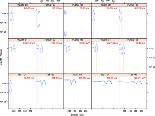
Figure 1: Attenuated subspectra of monoenergetic gamma emissions for ¹³¹I and ²³⁹Pu, on the logarithmic scale, whose branching ratios (probabilities of emission) are greater than $0.5\%$, under lead shielding with $x=0$ (i.e., no shielding, upper curves) and $x=10$ (lower curves).

We now present the statistical model for the pulse height spectrum recorded in a detector. Let $Y_{i}$ represent the photon count at the $i$th energy channel of a spectrometer, where $i=1,\ldots,N$. [For example, $N=1024$ channels over the energy range up to 3 megaelectron volt (MeV).] The photon counts are modeled as independent Poisson random variables, with the mean of $Y_{i}$ given by

$$\mu_{i}=\sum_{j=1}^{J}\sum_{l=1}^{p_{j}}S_{ijl}a_{jl},$$

where $\{S_{ijl},i=1,\ldots,N\}$ is the detector response function to the $l$th monoenergetic gamma ray emitted by the $j$th nuclide, $l=1,\ldots,p_{j},j=1,\ldots,J$. For simplicity, background radiation is included in the library of radionuclides postulated to be in the source, and it is indexed by $J$, so $p_{J}=1$. Here, $a_{jl}$ denotes the (relative) intensity of the $l$th monoenergetic gamma ray of the $j$th nuclide.

Suppose that a slab of known intervening material of a pure type, for example, lead, of thickness $t$ and density $\rho$ stands perpendicular to the path between a radioactive source and the spectrometer. The attenuation of the gamma ray depends on its energy and the intervening material. Let $I_{j0}$ be the initial emission intensity of the $j$th nuclei. The intervening material then attenuates the intensity of its $l$th monoenergetic gamma ray to $I_{jl}=I_{j0}\times e^{{-c_{jl}\times x}}$, where $c_{jl}$ (cm²/g) is the mass attenuation coefficient (see the NIST websites), and $x$ (g/cm²) is the mass thickness, that is, the product of the density $\rho$ and thickness $t$ of the intervening material. The attenuation formula can be extended to the case of multiple intervening materials (e.g., carbon and lead), say, $M$ of them each of mass thickness $x_{m}$, $m=1,\ldots,M$:

$$I_{jl}=I_{j0}\times e^{-\sum_{j=1}^{M}{c_{jlm}\times x_{m}}},$$

where $c_{jlm}$ is the mass attenuation coefficient, due to the $m$th intervening material, for the $l$th monoenergetic gamma ray emitted by the $j$th nuclide. Here, we have omitted possible down scattering of the gamma spectra by shielding materials of low atomic number; see Section 7.

Consequently, in the presence of $M$ known intervening materials of mass thickness $x_{m},m=1,\ldots,M$, the photon counts over the $N$ energy bins, ${\mathbf{Y}}=(Y_{1},\ldots,Y_{N})^{\top}$, are modeled as jointly independent Poisson random variables with the marginal distribution given by

$$Y_{i}\sim\operatorname{Poisson}\Biggl{(}\mu_{i}=\sum_{j=1}^{J}\sum_{l=1}^{p_{j}}S_{ijl}a_{jl}\Biggr{)},$$

where

$$a_{jl}=b_{j}\tau\exp\Biggl{(}-\sum_{m=1}^{M}c_{jlm}x_{m}\Biggr{)},$$

$b_{j}$ is the initial (unshielded) intensity of the $j$th nuclide per unit time, and $\tau$ is the detection time which, for the moment, is fixed. The background radiation (listed as the $J$th “nuclide” in the library) is not shielded, hence, $c_{J1m}\equiv 0$, for all $m=1,\ldots,M$. Note the number of energy bins, $N$, is generally fixed. However, the detection time can be increased without bound. So, the asymptotic properties of the proposed method will be developed in the framework of fixed $N$ but increasing $\tau$.

3 The Lagrange multiplier test

We consider the problem of testing for shielding of a radioactive source that possibly comprises a finite number of known radionuclides by $M$ known intervening materials of unknown mass thickness.The null hypothesis of no shielding is

$$H_{0}\dvtx\ x_{1}=x_{2}=\cdots=x_{M}=0,$$

that is, ${\mathbf{x}}=(x_{1},\ldots,x_{M})^{\top}=\mathbf{0}$, whereas the alternative hypothesis of shielding is

$$H_{1}\dvtx\mbox{ at least one of }x_{m}>0,\qquad m=1,2,\ldots,M.$$

A test for shielding may proceed via a likelihood ratio test which requires fitting the unshielded model under the null hypothesis and the general, shielded model. The fitting of the latter model is quite complex, owing to the nonlinear attenuation function. Thus, it is desirable to develop a test that does not require estimating the general model. Intuitively, under the null hypothesis, the constrained maximum likelihood estimator with $\mathbf{x}=0$ should be close to the unconstrained maximum likelihood estimator, but otherwise they diverge from each other. Hence, under the null (alternative) hypothesis, the partial derivative of the log-likelihood w.r.t. $\mathbf{x}$, evaluated at the constrained estimator, should be close to (diverge from) the zero vector. The Lagrange multiplier test quantifies the evidence against the null hypothesis in terms of some quadratic form of the preceding partial derivative that is designed to be asymptotically $\chi^{2}$-distributed under the null hypothesis.

We now elaborate the Lagrange multiplier (score) test. First, we derive the score, the Hessian matrix and the Fisher information. Write${\bolds{\phi}}=(x_{1},x_{2},\ldots,x_{M},b_{1},b_{2},\ldots,b_{J})^{\top}=({\mathbf{x}}^{\top},\mathbf{b}^{\top})^{\top}$, where ${\mathbf{x}}=(x_{1},\ldots,x_{M})^{\top}$ and $\mathbf{b}=(b_{1},b_{2},\ldots,b_{J})^{\top}$. Let $u_{ijl}=S_{ijl}b_{j}\exp(-\sum_{m=1}^{M}c_{jlm}x_{m})$, $t_{ijl}=\break S_{ijl}\exp(-\sum_{m=1}^{M}c_{jlm}x_{m})$ and $U_{i}=\sum_{j=1}^{J}\sum_{l=1}^{p_{j}}u_{ijl}$. Note that the attenuation coefficients $c_{jlm}$ are known for specified intervening materials. The log likelihood function is given by

$$L({\bolds{\phi}};\mathbf{Y})=-\tau\sum_{i=1}^{N}U_{i}+\sum_{i=1}^{N}Y_{i}\log(\tau U_{i})-\sum_{i=1}^{N}\log(Y_{i}!).$$

The score vector is given by $\mathcal{U}_{\tau}({\bolds{\phi}})=\nabla L({\bolds{\phi}};\mathbf{Y})=\bigl{[}{\mathcal{U}_{1,\tau}\atop\mathcal{U}_{2,\tau}}\bigr{]}$, where

$$\mathcal{U}_{1,\tau}=\biggl{(}\frac{\partial{L({\bolds{\phi}};\mathbf{Y})}}{\partial{x_{m^{\prime}}}},m^{\prime}=1,\ldots,M\biggr{)}^{\top}$$

and

$$\mathcal{U}_{2,\tau}=\biggl{(}\frac{\partial{L({\bolds{\phi}};\mathbf{Y})}}{\partial{b_{k}}},k=1,\ldots,J\biggr{)}^{\top},$$

with

$$\frac{\partial{L({\bolds{\phi}};\mathbf{Y})}}{\partial{x_{m^{\prime}}}} = \tau\sum_{i=1}^{N}\sum_{j=1}^{J}\sum_{l=1}^{p_{j}}u_{ijl}c_{jlm^{\prime}}$$

$${}-\sum_{i=1}^{N}Y_{i}U_{i}^{-1}{\sum_{j=1}^{J}\sum_{l=1}^{p_{j}}u_{ijl}c_{jlm^{\prime}}},\qquad m^{\prime}=1,\ldots,M$$

and

$$\frac{\partial{L({\bolds{\phi}};\mathbf{Y})}}{\partial{b_{k}}} = -\tau\sum_{i=1}^{N}\sum_{l=1}^{p_{k}}t_{ikl}$$

$${}+\sum_{i=1}^{N}Y_{i}U_{i}^{-1}{\sum_{l=1}^{p_{k}}t_{ikl}},\qquad k=1,\ldots,J.$$

The second derivatives equal

$$\frac{\partial^{2}{L({\bolds{\phi}};\mathbf{Y})}}{\partial{x_{m^{\prime\prime}}}\,\partial{x_{m^{\prime}}}} = -\tau\sum_{i=1}^{N}\sum_{j=1}^{J}\sum_{l=1}^{p_{j}}u_{ijl}c_{jlm^{\prime}}c_{jlm^{\prime\prime}}$$

$${}+\sum_{i=1}^{N}Y_{i}\Biggl{\{}U_{i}^{-1}\sum_{j=1}^{J}\sum_{l=1}^{p_{j}}u_{ijl}c_{jlm^{\prime}}c_{jlm^{\prime\prime}}$$

$$\hskip 45.0pt{}-U_{i}^{-2}\Biggl{(}\sum_{j=1}^{J}\sum_{l=1}^{p_{j}}u_{ijl}c_{jlm^{\prime}}\Biggr{)}\sum_{j=1}^{J}\sum_{l=1}^{p_{j}}u_{ijl}c_{jlm^{\prime\prime}}\Biggr{\}}$$

for $m^{\prime},m^{\prime\prime}=1,\ldots,M$,

$$\frac{\partial^{2}{L({\bolds{\phi}};\mathbf{Y})}}{\partial{x_{m^{\prime}}}\,\partial{b_{k}}} = \tau\sum_{i=1}^{N}\sum_{l=1}^{p_{k}}t_{ikl}c_{klm^{\prime}}$$

$${}+\sum_{i=1}^{N}Y_{i}\Biggl{\{}U_{i}^{-2}\Biggl{(}\sum_{j=1}^{J}\sum_{l=1}^{p_{j}}u_{ijl}c_{jlm^{\prime}}\Biggr{)}\sum_{l=1}^{p_{k}}t_{ikl}-U_{i}^{-1}\sum_{l=1}^{p_{k}}t_{ikl}c_{klm^{\prime}}\Biggr{\}}$$

for $m^{\prime}=1,\ldots,M$ and $k=1,\ldots,J$, and

$$\frac{\partial^{2}{L({\bolds{\phi}};\mathbf{Y})}}{\partial{b_{h}}\,\partial{b_{k}}}=-\sum_{i=1}^{N}Y_{i}U_{i}^{-2}{\Biggl{(}\sum_{l=1}^{p_{k}}t_{ikl}\Biggr{)}\Biggl{(}\sum_{l=1}^{p_{h}}t_{ihl}\Biggr{)}}$$

for $k,h=1,\ldots,J$.

Let

$$\mathcal{F}_{\tau}({\bolds{\phi}})=-\nabla^{2}L({\bolds{\phi}};\mathbf{Y})=\left[\matrix{\mathcal{F}_{11}&\mathcal{F}_{12}\vspace*{2pt}\cr\mathcal{F}_{21}&\mathcal{F}_{22}}\right]$$

be partitioned according to $\mathbf{x}$ and $\mathbf{b}$, where

$$\mathcal{F}_{11}=\biggl{(}-\frac{\partial^{2}{L({\bolds{\phi}};\mathbf{Y})}}{\partial{x_{m^{\prime\prime}}}\,\partial{x_{m^{\prime}}}}\biggr{)},\qquad\mathcal{F}_{12}=\biggl{(}-\frac{\partial^{2}{L({\bolds{\phi}};\mathbf{Y})}}{\partial{x_{m^{\prime}}}\,\partial{b_{k}}}\biggr{)},\qquad\mathcal{F}_{22}=\biggl{(}-\frac{\partial^{2}{L({\bolds{\phi}};\mathbf{Y})}}{\partial{b_{h}}\,\partial{b_{k}}}\biggr{)}$$

and $\mathcal{F}_{21}=\mathcal{F}_{21}^{\top}$.

Consequently, the Fisher information matrix equals

$$\mathcal{I}=\left[\matrix{\mathcal{I}_{11}&\mathcal{I}_{12}\vspace*{2pt}\cr\mathcal{I}_{21}&\mathcal{I}_{22}}\right]=\tau\left[\matrix{I_{11}&I_{12}\cr I_{21}&I_{22}}\right]=\tau I,$$

where the arguments $m^{\prime},m^{\prime\prime}$ below range from $1,\ldots,M$ and $k,h=1,\ldots,J$,

$$I_{11} = \biggl{[}E\biggl{(}-\frac{1}{\tau}\frac{\partial^{2}{L({\bolds{\phi}};\mathbf{Y})}}{\partial{x_{m^{\prime\prime}}}\,\partial{x_{m^{\prime}}}}\biggr{)}\biggr{]}$$

$$= \Biggl{[}\sum_{i=1}^{N}U_{i}^{-1}\Biggl{(}\sum_{j=1}^{J}\sum_{l=1}^{p_{j}}u_{ijl}c_{jlm^{\prime}}\Biggr{)}\Biggl{(}\sum_{j=1}^{J}\sum_{l=1}^{p_{j}}u_{ijl}c_{jlm^{\prime\prime}}\Biggr{)}\Biggr{]},$$

$$I_{21}^{\top}=I_{12} = \biggl{[}E\biggl{(}-\frac{1}{\tau}\frac{\partial^{2}{L({\bolds{\phi}};\mathbf{Y})}}{\partial{x_{m^{\prime}}}\,\partial{b_{k}}}\biggr{)}\biggr{]}$$

$$= \Biggl{[}-\sum_{i=1}^{N}U_{i}^{-1}\Biggl{(}\sum_{j=1}^{J}\sum_{l=1}^{p_{j}}u_{ijl}c_{jlm^{\prime}}\Biggr{)}\Biggl{(}\sum_{l=1}^{p_{k}}t_{ikl}\Biggr{)}\Biggr{]}$$

and

$$I_{22}=\biggl{[}E\biggl{(}-\frac{1}{\tau}\frac{\partial^{2}{L({\bolds{\phi}};\mathbf{Y})}}{\partial{b_{h}}\,\partial{b_{k}}}\biggr{)}\biggr{]}=\Biggl{[}\sum_{i=1}^{N}U_{i}^{-1}\Biggl{(}\sum_{l=1}^{p_{k}}t_{ikl}\Biggr{)}\Biggl{(}\sum_{l=1}^{p_{h}}t_{ihl}\Biggr{)}\Biggr{]}.$$

Let $\mathcal{U}_{1,\tau}(\tilde{{\bolds{\phi}}};\mathbf{Y})$ be an $M$-dimensional column vector with its $m$th element equal to $\frac{\partial{L(\tilde{{\bolds{\phi}}};\mathbf{Y})}}{\partial{x_{m}}}$. Let $\tilde{{\bolds{\phi}}}=(\mathbf{0}^{\top},\tilde{\mathbf{b}}^{\top})^{\top}=(0,\ldots,0,\tilde{b}_{1},\ldots\tilde{b}_{J})^{\top}$ be the constrained maximum likelihood estimator of ${\bolds{\phi}}$ under the null hypothesis. Note that $\tilde{\mathbf{b}}$ can be computed via the EM algorithm. Let $I^{11}$ be the $(1,1)$ block of the inverse of the Fisher information matrix $I$. The Lagrange multiplier (LM) test statistic equals

$$\xi_{\mathrm{LM}} = \frac{1}{\tau}{\mathcal{U}_{1,\tau}(\tilde{{\bolds{\phi}}};\mathbf{Y})}^{\top}I^{11}(\tilde{{\bolds{\phi}}})\mathcal{U}_{1,\tau}(\tilde{{\bolds{\phi}}};\mathbf{Y})$$

$$= \frac{1}{\tau}{\mathcal{U}_{1,\tau}(\tilde{{\bolds{\phi}}};\mathbf{Y})}^{\top}{\bigl{\{}I_{11}(\tilde{{\bolds{\phi}}})-I_{12}(\tilde{{\bolds{\phi}}})I^{-1}_{22}(\tilde{{\bolds{\phi}}})I_{21}(\tilde{{\bolds{\phi}}})\bigr{\}}}^{-1}\mathcal{U}_{1,\tau}(\tilde{{\bolds{\phi}}};\mathbf{Y}).$$

Below we show that the LM test statistic is asymptotically $\chi^{2}$ distributed and that the classical result on the asymptotic equivalence between the LM test, the likelihood ratio test and the Wald test holds, under general regularity conditions. Recall the likelihood ratio (LR) test statistic equals

$$\xi_{\mathrm{LR}}=2\bigl{\{}L(\hat{\bolds{\phi}})-L(\tilde{\bolds{\phi}})\bigr{\}},$$

where $\hat{\bolds{\phi}}=(\hat{\mathbf{x}}^{\top},\hat{\mathbf{b}}^{\top})^{\top}$ denotes the unconstrained ML estimator under the general hypothesis, and the Wald test statistic equals

$$\xi_{\mathrm{W}} = \sqrt{\tau}\hat{\mathbf{x}}^{\top}\bigl{\{}I^{11}(\hat{\bolds{\phi}})\bigr{\}}^{-1}\sqrt{\tau}\hat{\mathbf{x}}$$

$$= \tau\hat{\mathbf{x}}^{\top}{\bigl{\{}I_{11}(\hat{\bolds{\phi}})-I_{12}(\hat{\bolds{\phi}})I^{-1}_{22}(\hat{\bolds{\phi}})I_{21}(\hat{\bolds{\phi}})\bigr{\}}}\hat{\mathbf{x}}.$$

The following assumption is required for the asymptotic equivalence of the preceding tests under the null hypothesis: [(A1)]

The true mean unshielded spectrum is a positive function, that is, $\sum_{j=1}^{J}b_{j}S_{ij\bullet}>0$ for every energy channel $i=1,\ldots,N$, where $S_{ij\bullet}=\sum_{l=1}^{p_{j}}S_{ijl}$. Denote the partial derivatives of the mean spectrum w.r.t. $\mathbf{x}$ and $\mathbf{b}$, evaluated at $\mathbf{x}=0$ and at the true $\mathbf{b}$, by

$$\mathbf{v}_{q}=\Biggl{(}-\sum_{j=1}^{J}b_{j}\sum_{l=1}^{p_{j}}S_{ijl}c_{jlq},i=1,\ldots,N\Biggr{)}^{\top}$$

for $q=1,\ldots,M$ and

$$\mathbf{v}_{q+M}=(S_{iq\bullet},i=1,\ldots,N)^{\top}$$

for $q=1,\ldots,J$. Then the $M+J$ $\mathbf{v}$’s are linearly independent.

Note that $U_{i}$ is the mean of $Y_{i}$ at energy channel $i$. Under the null hypothesis of no shielding, $U_{i}=\sum_{j=1}^{J}b_{j}S_{ij\bullet}$, so (A1) states that the mean unshielded gamma-ray spectrum is a positive function. As a function of $i$, $S_{ij\bullet}$ is the overall DRF for the $j$th nuclide in the source, while $-\sum_{j=1}^{J}b_{j}\sum_{l=1}^{p_{j}}S_{ijl}c_{jlq}$ is the instantaneous reduction rate in the mean unshielded gamma-ray spectrum per unit mass thickness of the $q$th intervening material, evaluated under the hypothesis of no shielding. The linear independence assumption in (A1) thus formalizes the requirements that distinct radionuclides have unique gamma-ray signatures and distinct intervening materials admit unique attenuation patterns.

Theorem 3.1

Assuming (A1) and as the detection time $\tau\to\infty$, the LM test statistic, the Wald test statistic and the likelihood ratio test statistic all have asymptotic $\chi^{2}_{M}$ distributions under $H_{0}$: $\mathbf{x}=\mathbf{0}$.

We defer the proofs of all theoretical results to the supplemental article Chan et al. (2013). Arguably, (A1) is a mild assumption even though the second part fails if the attenuation functions (the attenuation coefficient as a function of the energy of the gamma ray) of the $M$ intervening materials are linearly dependent. Indeed, $M$ intervening materials with broadly similar attenuation functions may be practically approximated by one of the intervening materials with a modified mass thickness. Below, we illustrate that common intervening materials have broadly similar attenuation functions. Extensive simulation results reported below suggest that the LM test is robust to the nature and the number of intervening materials.

4 Local power of the LM test

In this section we derive the local power of the Lagrange multiplier test, the likelihood ratio test and the Wald test for testing

$$H_{0}\dvtx\bolds{\phi}=\bolds{\phi}_{0}$$

versus

$$H_{1,\tau}\dvtx\bolds{\phi}=\bolds{\phi}_{0}+\frac{\mathbf{h}}{\sqrt{\tau}},$$

where $\mathbf{h}=(\mathbf{h}_{1}^{\top},\mathbf{h}_{2}^{\top})^{\top}$, with the vector partition being similar to that of $\bolds{\phi}$. The following result shows that the tests reject a fixed alternative with probability approaching 1 as $\tau\to\infty$.

Theorem 4.1

Assume (A1) holds. Then as $\tau\to\infty$, the Lagrange multiplier test statistic, the likelihood ratio test statistic and the Wald test statistic have noncentral $\chi^{2}_{M}$ distributions with the noncentral parameter equal to $\mathbf{h}_{1}^{\top}(I_{11}-I_{12}I_{22}^{-1}I_{21})\mathbf{h}_{1}$ under $H_{1,\tau}\dvtx\bolds{\phi}=\bolds{\phi}_{0}+\frac{\mathbf{h}}{\sqrt{\tau}}$, where $\mathbf{h}=(\mathbf{h}_{1}^{\top},\mathbf{h}_{2}^{\top})^{\top}$.

5 Simulation studies

The modeled detector characteristics are those of a $3\times 3$ inch cylindrical NaI detector whose spectral response is degraded to a resolution at the Cesium 662 keV peak of 80 keV full width half maximum (FWHM) of the peak; consequently, the resolution is smaller at low energies, similar to real measurements. The resolution of the detector is degraded from that of a standard NaI detector to better approximate the response of a larger detector or different scintillation material that may be more appropriate for a drive through a portal system. The unshielded DRFs are constructed by assuming each source to be small and pure, placed at an arbitrary distance from the flat face of the detector with no materials intervening between the source and detector. This ignores the effects of attenuation and matrix effects in the source, but allows one to concentrate on identification in situations with poor detector resolution. The mean of the background signal used for the simulation is based upon a long-duration, measured background using a NaI detector at the US Military Academy Accelerator facility. This background is adjusted to include radiation from terrestrial sources pertaining to the ²³⁸U decay chain (e.g., ²¹⁴Pb, ²¹⁴Bi, ²⁰⁸Tl) that are degraded to the same resolution as the modeled detector; see Mitchell, Borgardt and Kouzes (2009). The data are further adjusted so that the variability of the counts about the long-term mean is consistent with a short duration measurement ($\sim$1 minute). The simulation of the possibly shielded data included this background and further assumed that there are two radionuclides in the source, namely, ¹³¹I and ²³⁹Pu, whose signatures are simulated as described above. ²³⁹Pu is chosen because it is the primary fissile isotope used for the production of nuclear weapons and the emissions from ²³⁹Pu are quite weak and easily attenuated since many of the lines are of relatively low energy. ¹³¹I is chosen because it is fairly common (and thus may not trigger a more extensive search) and has low energy emission lines that might be used to intentionally mask the signature from ²³⁹Pu. This scenario represents a possible method to hide the transport of ²³⁹Pu. The response of the detector is calculated for each emission line for each of the radionuclides separately. These detector response functions will also be referred to as the subspectra for each of the nuclei. The detector response includes such phenomena as photoelectric absorption, pair production, Compton scattering, backscattered photons, escape peaks and detector efficiency. Each of the subspectra is calculated in proportion to the branching ratios of the emission lines. Thus, in the absence of shielding, the mean total response for a given radionuclide is obtained by multiplying all of the constituent subspectra by the same constant and adding the resultant spectra. Notice that all the subspectra of ²³⁹Pu are under 300 keV and so are some subspectra of ¹³¹I.

Four common intervening materials, namely, carbon, concrete, lead and water are of interest. A plot of the mass attenuation coefficients (on log scale) against the energy of the monoenergetic gamma ray, under water, concrete, carbon and lead shielding for the two radionuclides ¹³¹I and ²³⁹Pu are presented in Figure 2. (The mass attenuation coefficients are obtained by spline interpolation based on the tables of mass attenuation coefficients posted on the NIST website.) The curves of mass attenuation coefficients for carbon, water and concrete shielding are quite similar. Lead has higher attenuation than the other three materials, at any energy level of the photon, but it also takes a broadly similar attenuation pattern.

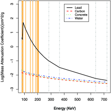
Figure 2: ¹³¹I and ²³⁹Pu mass attenuation coefficients, with vertical lines corresponding to the peak energy of each subspectrum of ²³⁹Pu and vertical dot-dashed lines corresponding to the peak energy of each subspectrum of ¹³¹I.

Simple intervening material

We first consider the case of a single intervening material, in which case simulation is done as follows: [1.]

Let $b_{1}=1$ be the coefficient of ¹³¹I, $b_{2}=0.15$ the coefficient of ²³⁹Pu, and $b_{3}=1$ that of the background.

Determine $c{}_{1l}$ and $c{}_{2l}$ (cm²/g), where $c{}_{1l}$ and $c{}_{2l}$ are the mass attenuation coefficients under the specified intervening material for each monoenergetic gamma ray of ¹³¹I and ²³⁹Pu in the library. Note the background is not attenuated by the shielding material so $c{}_{31}=0$.

Calculate $a_{1l}=b_{1}\tau\exp(-c_{1l}\times x)$ and $a_{2l}=b_{2}\tau\exp(-c_{2l}\times x)$ for each $x$, respectively, where $\tau=1$.

Simulate $Y_{i}$ as independent Poisson random variables with mean$\sum_{j=1}^{J}\sum_{l=1}^{p_{j}}S_{ijl}a_{jl}$. Note $J=3$ since we only have ¹³¹I, ²³⁹Pu and background. The parameter $x$ ranges from 0 to 30 (g/cm²).

Figure 1 shows, on the logarithmic scale, the attenuation of the mean subspectra of monoenergetic gamma emissions for ¹³¹I and ²³⁹Pu whose branching ratios are greater than $0.5\%$, contrasting the case under lead shielding with $x=10$ versus no shielding. In particular, the upper curve in each sub-figure there is the detector response function (on the logarithmic scale) to the monoenergetic gamma emission from the nuclide. Figure 3 shows those under carbon shielding.

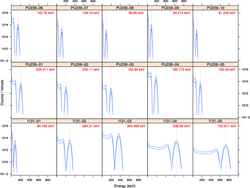
Figure 3: Attenuated subspectra of monoenergetic gamma emissions for ¹³¹I and ²³⁹Pu, on the logarithmic scale, whose branching ratios are greater than $0.5\%$, under carbon shielding with $x=0$ (i.e., no shielding, upper curves) and $x=10$ (lower curves).

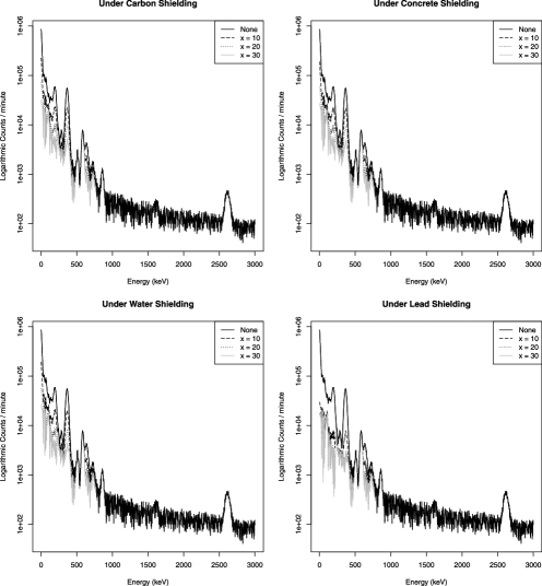
Figure 4: Simulated signals under shielding where the mass thickness $x$ is in g/cm².

A sample of simulated signals is presented in Figure 4 per intervening material. Empirical power and size of both tests are based on 2000 replications, with the empirical size checked against the nominal significance level of 0.05. The LM test statistics were computed with the constrained ML estimators obtained via the EM algorithm with the convergence criterion of the relative maximum change in the $L^{1}$ norm of the parameter estimate being less than $10^{-9}$, in all reported results; see the supplemental article Chan et al. (2013).

We first consider the case of carbon shielding. In practice, the nature of the intervening material is unknown. So we perform the LM test first assuming the intervening material is carbon and then do the same test assuming one of three other misspecified intervening materials, namely, concrete, lead and water. The derived asymptotic $\chi^{2}$ distribution for the LM test allows us to asymptotically calibrate the test, for example, by computing the approximate $p$-value based on the $\chi^{2}$ distribution. Moreover, that the limiting distribution is identical regardless of the true composition of the sources (true $\mathbf{b}$ value) under the null hypothesis justifies using the bootstrap for calibrating the LM test, which may be more accurate for low signal-to-noise cases.

The empirical sizes of the LM test for various settings and under the null hypothesis that $x=0$ at a level of 0.05 are presented in Table 1. All sizes are close to the nominal size of the test. An examination of quantile–quantile (q–q) plots (unreported) of the LM test statistic against the theoretical Chi-square distribution with one degree of freedom confirms the asymptotic Chi-square distribution. Note that the detection time is $\tau=1$ in all simulations, even though the theoretical results are derived under the assumption that $\tau\rightarrow\infty$. This suggests that the results apply even for short times $\tau$.

The empirical power curves for the nominal 0.05 LM test for attenuation due to carbon, water, concrete and lead are shown in Figure 5 when carbon is the true intervening material (top left), when concrete is the true intervening material (top right), when water is the true intervening material (bottom right), and when lead is the true intervening material (bottom left plot). Each plot gives power curves for $x$ ranging from 0 to 0.05 when the LM test is administered at the nominal 0.05 significance level. All power curves increase with increasing mass thickness, because greater mass thickness entails stronger shielding, resulting in higher power. The power curves for carbon, water and concrete shielding are of broadly similar shape. However, the power curve for detecting lead shielding has a different shape, as it approaches 100% power rather quickly. The shape difference in the power curves is due to the much stronger lead attenuation function that has a somewhat different shape; see Figure 2. We notice that the empirical power curves are almost identical for different combinations of true and presumed intervening materials, although the power is slightly decreased if the intervention material is misspecified. In other words, the test is robust to the nature of the intervening material, which likely owes to the fact that the attenuation functions of these four intervening materials have rather similar shapes.

Table 1: Empirical size of the LM test for shielding of Poisson signals from ¹³¹I, 0.15 ²³⁹Pu and background, for each of 4 intervening materials

Test	Carbon	Concrete	Lead	Water
LM	0.046	0.044	0.046	0.045

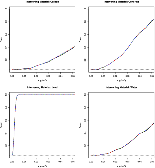
Figure 5: Empirical power curves when the true intervening material is carbon (top left), concrete (top right), water (bottom right) and lead (bottom left) for the LM test with $x$ ranging from 0 to 0.05 g/cm². The horizontal dashed lines show the 0.05 nominal level. The power curves for testing for attenuation by carbon (concrete, lead, water) are drawn as red dashed (green dotted, black solid, blue dot-dashed) lines and nearly coincide in most cases.

Composite intervening materials

Next, we consider the case of two intervening materials. There are six cases: carbon–lead shielding, concrete–lead shielding, water–lead shielding, water–carbon shielding, water–concrete shielding and concrete–carbon shielding. The data simulation scheme is similar to the case of the simple intervening material, with appropriate modifications as follows: [1.]

Determine $c{}_{1lm}$ and $c{}_{2lm}$, where $c{}_{1lm}$ and $c{}_{2lm}$ are the mass attenuation coefficients under the $m$th, $m=1,2$ intervening material for each monoenergetic gamma emission of ¹³¹I and ²³⁹Pu.

Find the mass thickness such that the empirical power is approximately 50% at the nominal 5% LM test for each intervening material alone. For each combination of two shielding materials, let $x_{M}$ denote the vector of their mass thickness so determined. We vary the vector of mass thickness as a multiple of $x_{M}$, with the multiple being 0 to 1 with increment by $1/19$, in total 20 of them.

Calculate $a_{1l}=b_{1}\tau\exp(-\sum_{m=1}^{2}c_{1lm}\times x_{m})$ and $a_{2l}=b_{2}\tau\times\break\exp(-\sum_{m=1}^{2}c_{2lm}\times x_{m})$ for each $x_{m},m=1,2$, respectively, and $\tau=1$.

Simulate $Y_{i}$ as independent Poisson random variables with mean$\sum_{j=1}^{J}\sum_{l=1}^{p_{j}}S_{ijl}a_{jl}$. Note $J=3$ since we only have ¹³¹I, ²³⁹Pu and background.

We performed the LM test for shielding by the two true intervening materials, but of unknown mass thickness. Then we repeated the LM test assuming simple shielding by one of the two shielding materials. The empirical sizes of the LM test for composite shielding by known intervening materials at the nominal level of 0.05 are presented in Table 2. They are close to the nominal size of the test, which is 0.05. In comparison, the empirical size is 0.046 for testing for simple shielding by lead.

Table 2: Empirical sizes for the LM test when the Poisson signals from ¹³¹I, 0.15 ²³⁹Pu and background are shielded by various combinations of intervening materials

Test	Carbon–Lead	Concrete–Lead	Water–Lead	Water–Carbon	Water–Concrete	Concrete–Carbon
LM	0.050	0.046	0.048	0.051	0.051	0.050

Figure 6 together with Figure 7 contrast the empirical power of the test for composite shielding by known intervening materials with those of tests for simple shielding by possibly misspecified materials. These figures suggest that, somewhat paradoxically, the LM test for simple shielding may be more powerful than the LM test for composite shielding by known intervening materials, even for tests for simple shielding by a misspecified material.

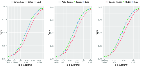
Figure 6: Empirical power when the true intervening materials are carbon and lead (left), water and carbon (middle) and concrete and carbon (right). The power curves for testing for simple shielding by carbon are drawn as green dashed lines, those of testing for simple shielding by lead as blue longdash lines, and those for testing for composite shielding by known materials as red solid lines.

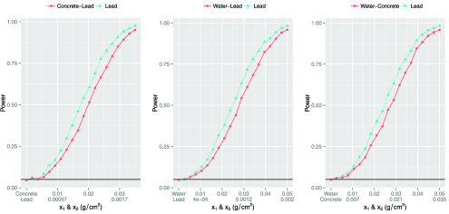
Figure 7: Empirical power when the true intervening materials are concrete and lead (left), water and lead (middle) and water and concrete (right). The power curves for testing for simple shielding by lead are drawn as blue dashed lines, and those for testing for composite shielding by known materials as red solid lines.

Below, we show that this phenomenon arises from the strong collinearity between the attenuation functions of commonly used intervening materials. Physically, the mass attenuation functions of intervening materials are generally decreasing functions of the photon energy, so they tend to be positively correlated. Hence, a nonphysical mass attenuation function is used for illustrating the problem of collinearity. For this purpose, we make up an artificial, nonphysical material whose mass attenuation function is “uncorrelated” with those of the intervening materials considered so far. We set the mass attenuation function of the artificial material to be $\exp(\sin(\mathit{En}))$, where $\mathit{En}$ is the energy level of the photon. The matrix of scatter plots between the mass attenuation functions of the artificial material together with the other four intervening materials is shown in Figure 8, which displays strong positive correlations among the attenuation functions of carbon, concrete, water and lead. However, there appears to be no relationship between the mass attenuation function of the artificial material and those of the other four materials. We then replicate the simulation experiment with signals simulated from ¹³¹I, $0.15^{239}$Pu and background, that are shielded by the artificial material and carbon, while we test for shielding by (i) the artificial material and carbon, and (ii) by one of the 5 possible intervening materials (carbon, lead, water, concrete and the artificial material) alone. The mass thicknesses of the true composite intervening materials are determined as before, with the maximum mass thickness of the artificial material being 0.005. Figure 9 displays the empirical powers of these tests based on 2000 replications, which now reveals that the test for shielding with the correct specification of the composite intervening materials (artificial-material–carbon) has higher power than any test for shielding by a single intervening material.

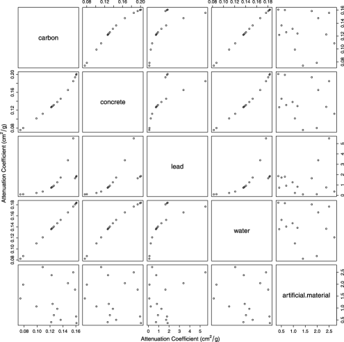
Figure 8: Scatter plot of the mass attenuation functions of carbon, concrete, water, lead and the artificial material.

Multicollinearity can be regarded as a form of ill-conditioning in the covariance matrix of the covariate. The condition number, which is defined as the square root of the ratio of the largest eigenvalue to the smallest eigenvalue of the covariance matrix, is often used to diagnose multicollinearity. A matrix with a high condition number (e.g., $>$30) indicates the presence of ill-conditioning. The severity of the multicollinearity increases with the condition number. The condition number of the Fisher information matrix, ${I_{11}(\tilde{{\bolds{\phi}}})-I_{12}(\tilde{{\bolds{\phi}}})I^{-1}_{22}(\tilde{{\bolds{\phi}}})I_{21}(\tilde{{\bolds{\phi}}})}$, for lead (mass thickness: $9.47\times 10^{-4}$) and carbon (mass thickness: $2.61\times 10^{-2}$) shielding is 185.8, while that of the artificial-material (mass thickness: $2.37\times 10^{-3}$) and carbon (mass thickness: $2.61\times 10^{-2}$) shielding is 12.88. This provides further evidence that the counterintuitive phenomenon arises from strong collinearity between the mass attenuation functions of commonly used intervening materials.

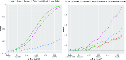
Figure 9: Empirical power curves when the true intervening materials are lead and carbon (left) and artificial material and carbon (right). In both cases, the empirical power curves of testing for simple shielding are almost the same, regardless of which intervening material is assumed in the test.

6 Sensitivity analysis

In order to assess the impacts of errors in the detector response functions (DRF) and background radiation on the proposed methods, we repeat the simulation study on the empirical power of the LM test for shielding of the source (¹³¹I and ²³⁹Pu) by carbon, with a similar setup as in the first simulation study in Section 4, but now with errors added to the DRFs and background radiation. To mimic systematic errors, we generate data with $S_{ijl}$ replaced by $\exp(m_{ijl})\times S_{ijl}$, where, as functions of $i$, $\{m_{ijl},i=1,\ldots,N\}$ are jointly independent integrated random walks. Specifically, $m_{i-2,j,l}-2m_{i-1,j,l}+m_{i,j,l}=c\eta_{i},i=N,N-1,\ldots,1$, with the boundary conditions that $m_{N+1,j,l}=m_{N+2,j,l}=0$, where $c>0$ is some scaling factor to make a certain signal to noise ratio and the $\eta$’s are independent standard normal variables. The integrated random walks are initiated from the high end of the spectrum to mimic the situation that systematic errors are largest in magnitude over the low end of the spectrum. In particular, this approach can account for errors due to neglecting Compton scattering by intervening materials, the modeling of which is complex, as it depends on the unknown geometric configuration encompassing the source, the detector and intervening materials. We use two values of $c$ that make the sample standard deviation of $\{m_{ijl},i=1,2,\ldots,N\}$ equal to $0.00025$ and $0.00035$, respectively, corresponding to roughly a maximum of 0.15% and 0.21% relative change in the pulse height of the 16 DRFs for the two isotopes plus background radiation, at each energy level. Data were simulated with the randomly modulated DRFs and background, but the tests assuming possible carbon shielding and correct source radionuclides are carried out assuming no DRF or background errors. Each experiment is replicated 6000 times.

Figure 10 plots the empirical power curves for $c=0,0.00025$ and $0.00035$, which show that errors in the DRFs and the background radiation inflated the size of the test, increasingly so with the magnitude of $c$. The case of $c=0$ corresponds to no shielding. The size-inflation problem can be corrected by finding the cutoff that makes the size of the test equal to the nominal 0.05. For example, for $c=0.00025$, the 0.05 quantile of the test statistic under the null hypothesis of no shielding, that is, $x=0$, is approximately $0.03234$, so the test can be corrected by rejecting the null hypothesis if the $p$-value of the LM test is less than 0.03504. Figure 10 shows that the size-correction procedure works at the expense of reducing the power of the test, with larger errors resulting in greater loss of power. Nonetheless, for small DFR and background errors, the corrected test still has good power for detecting shielding. An important research problem is to modify the proposed methods to make them powerful and yet robust to errors in the DRFs and background radiation.

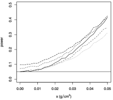
Figure 10: Empirical power of the LM test for shielding ¹³¹I and ²³⁹Pu by carbon with mass thickness $x$, with data generated with the DRFs modulated by independent additive integrated random walk errors on the logarithmic scale. Solid line: $c=0$, that is, no DRF or background errors; dashed line: $c=0.00025$; dotdash line: $c=0.00025$ with the test corrected to make the empirical size equal to the 0.05 nominal size; longdash line: $c=0.00035$; dotted line: $c=0.00035$ with the test corrected to make the empirical size equal to the 0.05 nominal size. Each experiment was replicated 6000 times.

7 Discussion

As noted, the LM test is attractive since only constrained maximum likelihood estimation is needed. Simulation results suggest that the LM test for simple shielding by lead is robust and powerful for testing for simple or composite shielding by four common intervening materials, even if the shielding materials do not contain lead. This result is practically significant, as we generally do not know the number and nature of the intervening materials. The usefulness of this robustness result can be broadened by checking whether or not it continues to hold with other shielding materials.

The problem of testing for shielding may also be addressed by a model selection approach using some information criterion, with the selection of the model with $x=0$ corresponding to no shielding. However, this requires fitting a nonlinear model with positive $x$, which may result in a difficult global optimization problem, especially in the case of composite shielding.

Implementing the proposed method in field applications, for example, cargo screening, requires further work to relax some restrictive assumptions of the proposed methods. A main problem is that besides attenuating gamma rays, intervening materials, especially those with low atomic number, such as carbon, water and concrete, may cause down scattering of the gamma spectrum via single or multiple external Compton scattering into the detector. Mitchell, Sanger and Marlow [(1989), equations (11)–(13)] proposed a semiparametric model for modeling Compton scattering between a monoenergetic gamma ray and materials outside the detector that enter into the spectrometer. However, the full specification of the semiparametric model is specific to the unknown geometry of the configuration encompassing the source, the detector and the shielding materials. Alternatively, down scattering may be studied by Monte Carlo techniques, for example, in MCNP and GEANT, but this does not yield a closed-form solution for the test statistics. Hence, down scattering due to Compton scattering external to the spectrometer cannot be directly incorporated in our proposed testing approach. While the impact of Compton scattering into the detector may be of secondary importance, its omission results in errors in the background radiation and may reduce the power of the test, as demonstrated in Section 6. Given the complexity needed for modeling external Compton scattering, it seems that the problem may be best mitigated by modifying the proposed methods to make them robust to errors in the background and the DRFs.

While our main concern is to detect special nuclear material (SNM) and so it is reasonable to consider only a few Pu isotopes and a few U isotopes, it is imperative to reduce false alarms due to the presence of other isotopes such as Neptunium (Np) and Americium (Am) that can be weaponized, or naturally occurring radioactive materials (NORM) such as granite, litter, etc. These “nuisance” isotopes and/or NORMs are less likely shielded deliberately, the presence of each of which is, hence, characterized by their unique overall DRF signature. The latter signature DRFs can then be additively augmented into the Poisson regression model, with their coefficients treated as nuisance parameters in the tests. The theoretical properties and practical performance of this approach for adjusting for nuisance radioactive materials constitute an interesting future research direction.

The proposed methods assume known sources of SNMs which are, however, generally unknown. One way to deal with this problem is to enumerate a list of interesting combinations of source SNM, perform the test for each such combination of source SNMs, and adjust for the multiplicity of tests, for instance, by the Bonferroni rule or some other schemes [Benjamini (2010)].

Background radiation generally varies over time, so an interesting problem is to devise a real-time updating scheme for background radiation that incorporates concurrent covariate information, for example, the vehicle type that may predict associated background suppression by vehicles in cargo screening [Lo Presti et al. (2006)], and to study the performance of the proposed methods using the background updating procedure.

Another future research problem is to detect shielding in primary screening with very low resolution gamma detectors.

[id=suppA] Proofs of Theorems 3.1 and 4.1 and constrained maximum likelihood estimation via the EM algorithm [doi]10.1214/13-AOAS704SUPP .pdf aoas704_supp.pdf This supplement contains (i) detailed proofs of Theorems 3.1 and 4.1, and (ii) an algorithm for constrained maximum likelihood estimation assuming no shielding.

References

- Allison et al. (2006) {barticle}[author] \bauthor\bsnmAllison, \bfnmJohn\binitsJ., \bauthor\bsnmAmako, \bfnmK.\binitsK., \bauthor\bsnmApostolakis, \bfnmJ.\binitsJ., \bauthor\bsnmAraujo, \bfnmH.\binitsH., \bauthor\bsnmDubois, \bfnmP. Arce\binitsP. A., \bauthor\bsnmAsai, \bfnmMe\binitsM., \bauthor\bsnmBarrand, \bfnmG. A. B. G.\binitsG. A. B. G., \bauthor\bsnmCapra, \bfnmR. A. C. R.\binitsR. A. C. R., \bauthor\bsnmChauvie, \bfnmS. A. C. S.\binitsS. A. C. S., \bauthor\bsnmChytracek, \bfnmR. A. C. R.\binitsR. A. C. R. \betalet al. (\byear2006). \btitleGeant4 developments and applications. \bjournalIEEE Transactions on Nuclear Science \bvolume53 \bpages270–278. \bptokimsref\endbibitem
- August and Whitlock (2005) {bmisc}[author] \bauthor\bsnmAugust, \bfnmR.\binitsR. and \bauthor\bsnmWhitlock, \bfnmR.\binitsR. (\byear2005). \bhowpublishedHELGA II: Autonomous passive detection of nuclear weapons materials. 2005 NRL Review, Naval Research Laboratory, Washington, DC. \bptokimsref\endbibitem
- Bai et al. (2011) {barticle}[author] \bauthor\bsnmBai, \bfnmE.\binitsE., \bauthor\bsnmChan, \bfnmKung-Sik\binitsK.-S., \bauthor\bsnmEichinger, \bfnmW.\binitsW. and \bauthor\bsnmKump, \bfnmP.\binitsP. (\byear2011). \btitleDetection of radionuclides from weak and poorly resolved spectra using Lasso and subsampling techniques. \bjournalRadiation Measurements \bvolume46 \bpages1138–1146. \bptokimsref\endbibitem
- Benjamini (2010) {barticle}[mr] \bauthor\bsnmBenjamini, \bfnmYoav\binitsY. (\byear2010). \btitleSimultaneous and selective inference: Current successes and future challenges. \bjournalBiom. J. \bvolume52 \bpages708–721. \biddoi=10.1002/bimj.200900299, issn=0323-3847, mr=2758547 \bptokimsref\endbibitem
- Bryan (2008) {bbook}[author] \bauthor\bsnmBryan, \bfnmJ. C.\binitsJ. C. (\byear2008). \btitleIntroduction to Nuclear Science. \bpublisherCRC Press, \blocationBoca Raton, FL. \bptokimsref\endbibitem
- Burr and Hamada (2009) {barticle}[author] \bauthor\bsnmBurr, \bfnmT.\binitsT. and \bauthor\bsnmHamada, \bfnmM. S.\binitsM. S. (\byear2009). \btitleRadio-isotope identification algorithms for NaI gamma spectra. \bjournalAlgorithms \bvolume2 \bpages339–360. \bptokimsref\endbibitem
- Cantone and Hoeschen (2011) {bbook}[author] \beditor\bsnmCantone, \bfnmM. C.\binitsM. C. and \beditor\bsnmHoeschen, \bfnmC.\binitsC., eds. (\byear2011). \btitleRadiation Physics for Nuclear Medicine. \bpublisherSpringer, \blocationBerlin. \bptokimsref\endbibitem
- Cashwell, Everett and Rechard (1957) {bmisc}[author] \bauthor\bsnmCashwell, \bfnmE D.\binitsE. D., \bauthor\bsnmEverett, \bfnmCornelius Joseph\binitsC. J. and \bauthor\bsnmRechard, \bfnmO W.\binitsO. W. (\byear1957). \bhowpublishedA practical manual on the Monte Carlo method for random walk problems. Los Alamos Scientific Lab., Los Alamos, New Mexico. Available at http://catalog.hathitrust.org/ Record/012213450. \bptokimsref\endbibitem
- Chan et al. (2012) {barticle}[author] \bauthor\bsnmChan, \bfnmKung-Sik\binitsK.-S., \bauthor\bsnmLi, \bfnmJ.\binitsJ., \bauthor\bsnmEichinger, \bfnmW.\binitsW. and \bauthor\bsnmBai, \bfnmE.\binitsE. (\byear2012). \btitleA new physics-based method for detecting weak nuclear signals via spectral decomposition. \bjournalNuclear Instruments and Methods in Physics Research Section A \bvolume667 \bpages16–25. \bptokimsref\endbibitem
- Chan et al. (2013) {bmisc}[author] \bauthor\bsnmChan, \bfnmKung-Sik\binitsK.-S., \bauthor\bsnmLi, \bfnmJinzheng\binitsJ., \bauthor\bsnmEichinger, \bfnmWilliam\binitsW. and \bauthor\bsnmBai, \bfnmErWei\binitsE. (\byear2013). \btitleSupplement to “Testing for shielding of special nuclear weapon materials.” DOI:\doiurl10.1214/13-AOAS704SUPP. \bptokimsref\endbibitem
- Fetter et al. (1990) {barticle}[pbm] \bauthor\bsnmFetter, \bfnmS.\binitsS., \bauthor\bsnmCochran, \bfnmT. B.\binitsT. B., \bauthor\bsnmGrodzins, \bfnmL.\binitsL., \bauthor\bsnmLynch, \bfnmH. L.\binitsH. L. and \bauthor\bsnmZucker, \bfnmM. S.\binitsM. S. (\byear1990). \btitleGamma-ray measurements of a Soviet cruise-missile warhead. \bjournalScience \bvolume248 \bpages828–834. \biddoi=10.1126/science.248.4957.828, issn=0036-8075, pii=248/4957/828, pmid=17811831 \bptokimsref\endbibitem
- Gardner and Xu (2009) {barticle}[author] \bauthor\bsnmGardner, \bfnmR. P.\binitsR. P. and \bauthor\bsnmXu, \bfnmL.\binitsL. (\byear2009). \btitleStatus of the Monte Carlo library least-squares (MCLLS) approach for nonlinear radiation analyzer problems. \bjournalRadiation Physics and Chemistry \bvolume78 \bpages843–851. \bptokimsref\endbibitem
- Jarman et al. (2003) {barticle}[author] \bauthor\bsnmJarman, \bfnmK. H.\binitsK. H., \bauthor\bsnmDaly, \bfnmD. S.\binitsD. S., \bauthor\bsnmAnderson, \bfnmK. K.\binitsK. K. and \bauthor\bsnmWahl, \bfnmK. L.\binitsK. L. (\byear2003). \btitleA new approach to automated peak detection. \bjournalChemometrics and Intelligent Laboratory Systems \bvolume69 \bpages61–76. \bptokimsref\endbibitem
- Kump et al. (2012) {barticle}[mr] \bauthor\bsnmKump, \bfnmPaul\binitsP., \bauthor\bsnmBai, \bfnmEr-Wei\binitsE.-W., \bauthor\bsnmChan, \bfnmKung-sik\binitsK.-s., \bauthor\bsnmEichinger, \bfnmBill\binitsB. and \bauthor\bsnmLi, \bfnmKang\binitsK. (\byear2012). \btitleVariable selection via RIVAL (removing irrelevant variables amidst Lasso iterations) and its application to nuclear material detection. \bjournalAutomatica J. IFAC \bvolume48 \bpages2107–2115. \biddoi=10.1016/j.automatica.2012.06.051, issn=0005-1098, mr=2956886 \bptokimsref\endbibitem
- Lo Presti et al. (2006) {barticle}[author] \bauthor\bsnmLo Presti, \bfnmC. A.\binitsC. A., \bauthor\bsnmWeier, \bfnmD.\binitsD., \bauthor\bsnmKouzes, \bfnmR.\binitsR. and \bauthor\bsnmSchweppe, \bfnmJ.\binitsJ. (\byear2006). \btitleBaseline suppression of vehicle portal monitor gamma count profiles: A characterization study. \bjournalNuclear Instruments and Methods in Physics Research Section A \bvolume562 \bpages281–297. \bptokimsref\endbibitem
- Maher and Wikibooks Contributors (2008) {bmisc}[author] \bauthor\bsnmMaher, \bfnmK.\binitsK. and \borganizationWikibooks Contributors (\byear2008). \bhowpublishedBasic physics of nuclear medicine. Libronomia company. Available at http://en.wikibooks.org/wiki/Basic_Physics_of_ Nuclear_Medicine. \bptokimsref\endbibitem
- Marshall and Zumberge (1989) {barticle}[author] \bauthor\bsnmMarshall, \bfnmJ. H.\binitsJ. H. and \bauthor\bsnmZumberge, \bfnmJ. F.\binitsJ. F. (\byear1989). \btitleOn-line measurements of bulk coal using prompt gamma neutron activation analysis. \bjournalNuclear Geophysics \bvolume3 \bpages445–459. \bptokimsref\endbibitem
- Medalia (2009) {bmisc}[author] \bauthor\bsnmMedalia, \bfnmJ.\binitsJ. (\byear2009). \bhowpublishedDetection of nuclear weapons and materials: Science, technologies, observations. Technical Report No. R40154, CRS report for Congress. \bptokimsref\endbibitem
- Mitchell, Borgardt and Kouzes (2009) {bmisc}[author] \bauthor\bsnmMitchell, \bfnmAllison L.\binitsA. L., \bauthor\bsnmBorgardt, \bfnmJames D.\binitsJ. D. and \bauthor\bsnmKouzes, \bfnmRichard T.\binitsR. T. (\byear2009). \bhowpublishedSkyshine contribution to gamma ray background between 0 and 4 MeV. Pacific Northwest National Laboratory. Available at http://www.pnl.gov/main/publications/external/ technical_reports/PNNL-18666.pdf. \bptokimsref\endbibitem
- Mitchell, Sanger and Marlow (1989) {barticle}[author] \bauthor\bsnmMitchell, \bfnmDean J.\binitsD. J., \bauthor\bsnmSanger, \bfnmHoward M.\binitsH. M. and \bauthor\bsnmMarlow, \bfnmKeith W.\binitsK. W. (\byear1989). \btitleGamma-ray response functions for scintillation and semiconductor detectors. \bjournalNuclear Instruments and Methods In Physics Research Section A \bvolume276 \bpages574–556. \bptokimsref\endbibitem
- Moss et al. (2002) {bmisc}[author] \bauthor\bsnmMoss, \bfnmJ.\binitsJ., \bauthor\bsnmGeesaman, \bfnmD.\binitsD., \bauthor\bsnmSchroeder, \bfnmL.\binitsL., \bauthor\bsnmSimon-Gillo, \bfnmJ.\binitsJ. and \bauthor\bsnmKeister, \bfnmB.\binitsB. (\byear2002). \bhowpublishedReport on the workshop on the role of the nuclear physics research community in combating terrorism. Report No. DOE/SC-0062, U.S. Department of Energy, Washington, DC. \bptokimsref\endbibitem
- Smith and Lucas (2002) {bmisc}[author] \bauthor\bsnmSmith, \bfnmH. A.\binitsH. A. \bsuffixJr. and \bauthor\bsnmLucas, \bfnmM.\binitsM. (\byear2002). \bhowpublishedGamma-ray detectors. Los Alamos Technical reports, Federation of American Scientists. Available at http://www.lanl.gov/ orgs/n/n1/panda/00326398.pdf. \bptokimsref\endbibitem