Derivation of the Lifshitz-Matsubara sum formula for the Casimir pressure between metallic plane mirrors

Abstract

We carefully re-examine the conditions of validity for the consistent derivation of the Lifshitz-Matsubara sum formula for the Casimir pressure between metallic plane mirrors. We recover the usual expression for the lossy Drude model, but not for the lossless plasma model. We give an interpretation of this new result in terms of the modes associated with the Foucault currents which play a role in the limit of vanishing losses, in contrast to common expectations.

I Introduction

The Casimir force Casimir1948 is a manifestation of vacuum field fluctuations Milton2001 which is now measured with a good experimental precision in various experiments Klimchitskaya2009 ; Lamoreaux2011 ; Capasso2011 ; Decca2011 . However, the comparison of experimental results with theoretical predictions remains a matter of debate Klimchitskaya2006 ; Brevik2006 ; Lambrecht2011 . The original Casimir formula had a universal form, with the pressure between two plane plates being $P=-\hbar c\pi^{2}/240L^{4}$ as a function of the inter-plate distance $L$, because the mirrors were idealized as perfectly reflecting and thermal fluctuations were ignored. But experiments are performed with imperfect reflectors, at room temperature, so that the experimental results have to be compared with the Lifshitz formulas Lifshitz1956 ; Dzyaloshinskii1961 which take these effects into account.

Most experiments are performed with mirrors covered by thick layers of gold, and their optical properties are described by reflection amplitudes calculated from Fresnel equations at the interfaces between vacuum and metallic bulks Jaekel1991 . These reflection amplitudes are deduced from a frequency-dependent dielectric function $\varepsilon(\omega)$, which is the sum of contributions corresponding to bound electrons and conduction electrons. The function $\varepsilon(\omega)$ is deduced from tabulated optical data Lambrecht2000 ; Svetovoy2008 and extrapolated to low frequencies by using the Drude model for describing the conductivity of gold, $\sigma(\omega)=\omega_{\mathrm{p}}^{2}/(\gamma-{i}\omega)$, where $\omega_{\mathrm{p}}$ is the plasma frequency and $\gamma$ the damping parameter. This model incorporates the important fact that gold has a finite static conductivity $\sigma_{0}=\omega_{\mathrm{p}}^{2}/\gamma$.

The limiting case of a lossless plasma of conduction electrons ($\gamma=0$) is also often considered. This model cannot be an accurate description of metallic mirrors as it contradicts the fact that gold has a finite static conductivity while leading to a poor extrapolation of tabulated optical data. However, as $\gamma$ is much smaller than $\omega_{\mathrm{p}}$ for a good metal such as gold and the effect of dissipation is appreciable only at low frequencies $\omega\lesssim\gamma$ where $\varepsilon$ is very large for both models, one might expect that dissipation does not affect significantly the value of the Casimir force. This naive expectation is met at small distances or low temperatures but not in the general case. In fact, dissipation has a significant effect on the value of the Casimir force at room temperature at distances accessible in experiments Bostrom2000 ; Ingold2009 ; Brevik2014 . Furthermore, some experimental results appear to lie closer to the predictions of the lossless plasma model than to that of the dissipative Drude model Decca2007prd ; Decca2007epj ; Chang2012 . Other experiments at larger distances, $L>1\mu$m, have led to a better agreement with the dissipative model Sushkov2011 ; Milton2011 , at the price of a large correction due to the effect of electrostatic patches Kim2010 . This weird status of theory-experiment comparison has led to a large number of contributions, and many references can be found in the lecture notes Reynaud2014 . Among a variety of ideas, it has been suggested that the Lifshitz formulas might not be valid for dissipative media Bordag2011 .

The aim of the present paper is to check carefully the conditions of validity for the whole derivation of the Lifshitz formulas for the Casimir pressure between metallic plane mirrors, in particular for the two cases of the lossy Drude model and lossless plasma model. We focus attention on the questions related to the discontinuities appearing at the limit $\gamma\to 0$ of vanishing dissipation. In particular, we discuss with great care the equivalence of two kinds of Lifshitz formulas. The first one, which we will call the Lifshitz formula in the following, is an integral over all field modes characterized by real frequencies, while the second one, which we will call the Lifshitz-Matsubara formula, is a discrete sum over purely imaginary Matsubara frequencies Matsubara1955 .

We focus the discussion on the case of plane mirrors made of non-magnetic matter. We do not treat the problems associated with experiments performed in the plane-sphere geometry and also disregard the discussion of possible systematic effects in the theory-experiment comparison. References can be found in Lambrecht2011 ; Reynaud2014 for general discussions, in Banishev2012 ; Banishev2013 for experiments with magnetic mirrors, in Behunin2012 and Broer2012 for systematic effects due to electrostatic patches and roughness respectively.

II The Casimir radiation pressure between plane mirrors

We consider two plane and parallel mirrors placed in electromagnetic vacuum and forming a Fabry-Perot cavity. All fields in the outer or inner regions of this cavity can be deduced from the reflection amplitudes of the mirrors. The radiation pressures are different on the inner and outer sides of the mirrors, and the Casimir force is just the result of this difference integrated over all field modes Jaekel1991 . This approach is valid for lossy as well as lossless mirrors Genet2003 ; Lambrecht2006 , provided thermal equilibrium holds for the whole system, so that all input fluctuations, coming from electromagnetic fields, electrons, phonons or any loss mechanism, correspond to the same temperature $T$. The expression, to be written in the next paragraph, is valid and regular for any optical model of mirrors obeying causality and high frequency transparency properties. It reproduces the Lifshitz formulas Lifshitz1956 ; Dzyaloshinskii1961 when the mirrors are described by reflection amplitudes deduced from Fresnel equations, and also goes to the ideal Casimir expression when the mirrors tend to perfect reflection Schwinger1978 .

The expression obtained in this manner for the Casimir pressure $P$ is a sum over all modes, that is, an integral over the field frequency $\omega$ and the transverse components $\mathbf{k}$ of the wavevector and a sum over the polarizations $\varsigma$

$$P=\sum_{\mathbf{k}}\sum_{\varsigma}{\int}_{0}^{\infty}\frac{\mathrm{d}\omega}{2\pi}~{}\hbar k_{z}\left(g_{\mathbf{k}}^{\varsigma}(\omega)-1\right)C(\omega)~{},$$ (1)

$$g_{\mathbf{k}}^{\varsigma}(\omega)\equiv\frac{1-|\rho_{\mathbf{k}}^{\varsigma}(\omega)|^{2}}{|1-\rho_{\mathbf{k}}^{\varsigma}(\omega)|^{2}}~{},\;\rho_{\mathbf{k}}^{\varsigma}(\omega)\equiv\left(r_{\mathbf{k}}^{\varsigma}(\omega)\right)^{2}e^{2{i}k_{z}L}~{},$$

$$C(\omega)\equiv\coth\frac{\hbar\omega}{2k_{\mathrm{B}}T}=1+2n_{\omega}~{},\;n_{\omega}=\frac{1}{\exp\frac{\hbar\omega}{k_{\mathrm{B}}T}-1}~{}.$$

The sum over $\mathbf{k}$ is in fact a double integral over the components $(k_{x},k_{y})$ in the plane of the mirror (with the normal to the cavity along the $z$-direction) $\sum_{\mathbf{k}}\equiv\iint\mathrm{d}k_{x}\mathrm{d}k_{y}/(4\pi^{2})$ while the sum over $\varsigma$ is on TM (transverse magnetic) and TE (transverse electric) polarizations. The function $C(\omega)$ represents the equivalent number of photons per mode corresponding to vacuum and thermal fluctuations which impinge the cavity from its two sides (with $n_{\omega}$ the number of thermal photons in Planck’s law). The function $g_{\mathbf{k}}^{\varsigma}(\omega)$ is the ratio of the energy density inside the cavity to that outside for a given mode. It is deduced from the reflection amplitudes $r_{\mathbf{k}}^{\varsigma}(\omega)$ of the two mirrors, supposed to be identical for the sake of simplicity, and the propagation factor $\exp(2{i}k_{z}L)$, with $k_{z}$ the longitudinal component of the wavevector. The integral over frequencies includes the contributions of propagative ($\omega>c|\mathbf{k}|$) and evanescent ($\omega<c|\mathbf{k}|$) waves, with $k_{z}=\sqrt{\omega^{2}/c^{2}-\mathbf{k}^{2}}$ and $k_{z}={i}\sqrt{\mathbf{k}^{2}-\omega^{2}/c^{2}}$ respectively. Transverse wavevectors and polarizations are preserved in the situation considered in the present paper, and thus remain spectators throughout the discussions.

Resonant modes correspond to an increase of energy in the cavity with $g_{\mathbf{k}}^{\varsigma}(\omega)>1$ and they produce repulsive contributions to the pressure. In contrast, modes out of resonance correspond to a decrease of energy in the cavity with $g_{\mathbf{k}}^{\varsigma}(\omega)<1$ and produce attractive contributions. The net pressure is the balance of all contributions after integration over modes. It is finite for any model of mirrors and attractive between two non-magnetic mirrors. These properties are seen more easily by rewriting the pressure $P$ as a Matsubara sum, which is done in the following by rewriting (1) in terms of an analytic function.

To this end, we introduce the closed loop function $f_{\mathbf{k}}^{\varsigma}(\omega)$ which is a retarded causal function associated with the Fabry-Perot cavity simply expressed Jaekel1991 in terms of the open loop function $\rho_{\mathbf{k}}^{\varsigma}(\omega)$

$$g_{\mathbf{k}}^{\varsigma}(\omega)=1+f_{\mathbf{k}}^{\varsigma}(\omega)+(f_{\mathbf{k}}^{\varsigma}(\omega))^{\ast}=1+f_{\mathbf{k}}^{\varsigma}(\omega)+f_{\mathbf{k}}^{\varsigma}(-\omega)~{},$$

$$f_{\mathbf{k}}^{\varsigma}(\omega)\equiv\frac{\rho_{\mathbf{k}}^{\varsigma}(\omega)}{1-\rho_{\mathbf{k}}^{\varsigma}(\omega)}~{}.$$ (2)

We then use the properties of this function to deduce equivalent expressions of the Casimir pressure

$$P=\sum_{\mathbf{k,\varsigma}}\int_{0}^{\infty}\frac{\mathrm{d}\omega}{2\pi}~{}2\mathrm{Re}[p_{\mathbf{k}}^{\varsigma}]=\sum_{\mathbf{k,\varsigma}}\int_{-\infty}^{\infty}\frac{\mathrm{d}\omega}{2\pi}\mathrm{Re}[p_{\mathbf{k}}^{\varsigma}]~{},$$

$$p_{\mathbf{k}}^{\varsigma}(\omega)\equiv\hbar k_{z}f_{\mathbf{k}}^{\varsigma}(\omega)C(\omega)~{}.$$ (3)

In the following, we will consider the contribution to the Casimir pressure $P$ for given values $\varsigma,\mathbf{k}$ as the integral over the real axis of the function $p_{\mathbf{k}}^{\varsigma}$, and we will use its analyticity properties. To this end, we will add to the integral the contribution from its imaginary part $\mathrm{Im}[p_{\mathbf{k}}^{\varsigma}]$. As the latter shows singularities on the real axis, a proper definition of the integral will require the use of Cauchy’s principal value as discussed further below.

In order to exploit analytic properties, we introduce the complex variable $z=\omega+i\xi$ extending $\omega$ to the complex plane. The function $f_{\mathbf{k}}^{\varsigma}$ is defined from causal reflection amplitudes and propagation factors, and has its poles in the lower half of the complex plane which correspond to resonances of the Fabry-Perot cavity. Meanwhile the function $C$ has its poles at the Matsubara frequencies regularly spaced on the imaginary axis

$$z_{n}={i}\xi_{n}\quad,\;\xi_{n}=n\frac{2\pi k_{\mathrm{B}}T}{\hbar}~{}.$$ (4)

Occasionally, we will also have to take care of the branch cuts in $p_{\mathbf{k}}^{\varsigma}$ arising from the term $k_{z}$.

We then transform the Lifshitz formula (II) into a Lifshitz-Matsubara expression by a proper application of Cauchy’s residue theorem. The new expression is a sum of the residues of $p_{\mathbf{k}}^{\varsigma}$ at the Matsubara poles

$$P=-2k_{\mathrm{B}}T\sum_{\mathbf{k}}\sum_{\varsigma}\sum_{n}^{\prime}\kappa_{n}~{}f_{\mathbf{k}}^{\varsigma}[{i}\xi_{n}]~{},$$ (5)

$$\kappa_{n}=\sqrt{\mathbf{k}^{2}+\frac{\xi_{n}^{2}}{c^{2}}}~{}.$$

The symbol $\kappa_{n}$ corresponds to the continuation of $k_{z}$ to the Matsubara poles on the imaginary axis while the primed sum symbol means that the contribution of the zeroth pole $n=0$ is counted with only one half weight

$$\sum_{n}^{\prime}\varphi(n)\equiv\frac{1}{2}\varphi(0)+\sum_{n=1}^{\infty}\varphi(n)~{}.$$ (6)

The two formulas (II) and (5) are commonly considered as completely equivalent expressions of a single quantity, the Casimir pressure. In the next sections, we check carefully the conditions of validity of this equivalence property and prove that they are indeed met when the Drude model is used, but not when the lossless plasma model is used. We also give an interpretation of the difference.

III The Drude model

We come now to the discussion of mirrors described by the Drude model. To be specific, we model the permittivity of the metallic slab as

$$\varepsilon(\omega)=1-\frac{\omega_{\mathrm{p}}^{2}}{\omega(\omega+i\gamma)}~{}.$$ (7)

We thus disregard the contribution of bound electrons which do not play an important role in discussions focused around zero frequency. Of course, the contribution of bound electrons is taken into account in the comparison of experiment and theory Decca2007prd .

We consider that the slabs are thick enough so that the reflection amplitudes are given by Fresnel equations at the first interface

$$r_{\mathbf{k}}^{\mathrm{TE}}(\omega)=\frac{k_{z}-K_{z}}{k_{z}+K_{z}}~{},\;r_{\mathbf{k}}^{\mathrm{TM}}(\omega)=\frac{\varepsilon k_{z}-K_{z}}{\varepsilon k_{z}+K_{z}}~{},$$ (8)

where $K_{z}$ and $k_{z}$ are the longitudinal wavevectors in matter and vacuum respectively, that is for propagating waves

$$K_{z}=\sqrt{\varepsilon\frac{\omega^{2}}{c^{2}}-\mathbf{k}^{2}}~{},\;k_{z}=\sqrt{\frac{\omega^{2}}{c^{2}}-\mathbf{k}^{2}}~{}.$$ (9)

We now enter into a more detailed discussion of the poles of the functions $f_{\mathbf{k}}^{\varsigma}$, which are the resonances of the Fabry-Perot cavity, and lie in the lower half of the complex plane $\mathrm{Im}z<0$.

In the TM case, there are propagating Fabry-Perot modes quantized thanks to reflection on the mirrors, as well as modes due to hybridization of the surface plasmons living at the interfaces between vacuum and each metallic slab, which are coupled by the evanescent modes between the two slabs Intravaia2005 ; Intravaia2007 . The so-called $\omega_{-}$ mode is always evanescent with an attractive contribution to the pressure (contrary to any other modes whose contributions are always repulsive), while the $\omega_{+}$ mode can also be considered as the first of the set of Fabry-Perot modes, with a transition from the propagative to the evanescent sector as a function of $\mathbf{k}$. Finally, there exists modes associated with Foucault currents which lie on the negative imaginary axis.

In the TE case, the situation is similar for the propagating Fabry-Perot modes, there are no plasmonic modes but there also exist modes arising from the interaction between the Foucault currents living in the two slabs Intravaia2009 ; Intravaia2010 . All poles of $f_{\mathbf{k}}^{\varsigma}$ are represented as the red dots on Fig. 1 for $\varsigma=$ TM and TE on the top and bottom plot respectively. The poles of $C$ are represented as the black dots on the figures and the contours used below for the application of Cauchy’s residue theorem are also shown. The plots are drawn for exaggerated values of the parameter $\gamma$, in order to show that the red dots are below the real axis, thanks to the finite value of $\gamma$.

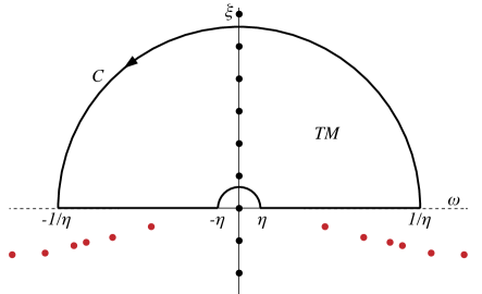
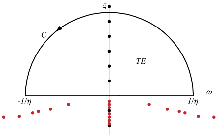
Figure 1: Poles of the function $f_{\mathbf{k}}^{\mathrm{TM}}(z)$ (top plot) and $f_{\mathbf{k}}^{\mathrm{TE}}(z)$ (bottom plot) represented as the red dots for metallic slabs described by the Drude model. Black dots are the poles due to $C(z)$. The contours used for the application of Cauchy’s theorem are also shown. The contours pass above the branch line associated with $k_{z}$ which runs on the real axis for $\omega^{2}>c^{2}\mathbf{k}^{2}$. [Colors online]

The comparison of the two figures shows important differences between the two cases. For the TE polarization, there is no pole at the origin $z=0$, because the behavior of $k_{z}f_{\mathbf{k}}^{\mathrm{TE}}\propto z^{2}$ around this point leads to the disappearance of the pole in $C(z)\propto 1/z$. We note at this point that the Foucault modes have been shown on Fig. 1 as a discrete set of poles, which corresponds to the case of metallic slabs of finite width $d$. This point is discussed in more detail in the next section.

Before going further, we have to study the parity properties of the functions involved in this discussion. We note that the permittivity is a real function in the space-time domain, so that $\left(\varepsilon(\omega)\right)^{\ast}=\varepsilon(-\omega)$. Our choice of definition for the square roots is such that $\left(k_{z}(\omega)\right)^{\ast}=-k_{z}(-\omega)$, and it follows that $\left(p_{\mathbf{k}}^{\varsigma}(\omega)\right)^{\ast}=p_{\mathbf{k}}^{\varsigma}(-\omega)$. Then, the real parts of $p_{\mathbf{k}}^{\varsigma}$ are even functions of $\omega$ and their imaginary parts are odd functions. After a continuation to the complex plane, this property is read as a mirror symmetry property with respect to the imaginary axis $\left(p_{\mathbf{k}}^{\varsigma}(z)\right)^{\ast}=p_{\mathbf{k}}^{\varsigma}(-z^{\ast})$, so that the positions of poles and zeros of these functions are symmetric with respect to the imaginary axis.

Using these parity properties as well as the properties already discussed, we deduce

$$\int_{-\infty}^{\infty}\mathrm{Re}[p_{\mathbf{k}}^{\mathrm{TE}}(\omega)]\frac{\mathrm{d}\omega}{2\pi}=2\int_{0}^{\infty}\mathrm{Re}[p_{\mathbf{k}}^{\mathrm{TE}}(\omega)]\frac{\mathrm{d}\omega}{2\pi}~{},$$

$$\int_{-\infty}^{\infty}\mathrm{Im}[p_{\mathbf{k}}^{\mathrm{TE}}(\omega)]\frac{\mathrm{d}\omega}{2\pi}=0~{},$$

$$\int_{-\infty}^{\infty}\mathrm{Re}[p_{\mathbf{k}}^{\mathrm{TM}}(\omega)]\frac{\mathrm{d}\omega}{2\pi}=2\int_{0}^{\infty}\mathrm{Re}[p_{\mathbf{k}}^{\mathrm{TM}}(\omega)]\frac{\mathrm{d}\omega}{2\pi}~{},$$

$$\mathcal{P}\int_{-\infty}^{\infty}\mathrm{Im}[p_{\mathbf{k}}^{\mathrm{TM}}(\omega)]\frac{\mathrm{d}\omega}{2\pi}=0~{}.$$ (10)

As already mentioned, $\mathrm{Im}[p_{\mathbf{k}}^{\mathrm{TM}}]$ has a $1/\omega$ singularity at the origin from the hyperbolic cotangent so that the proper definition of the last equation above has to be understood as a Cauchy’s principal value $\mathcal{P}$. For the other integrals, the functions are regular at the origin and the principal value is not needed. For a singularity at a point $c$ in the domain of integration $\left[a,b\right]$, Cauchy’s principal value, represented by the symbol $\mathcal{P}$, is defined as

$$\mathcal{P}\int_{a}^{b}\varphi(\omega)\text{d}\omega=\lim_{\epsilon\to 0^{+}}\left[\int_{a}^{c-\epsilon}+\int_{c+\epsilon}^{b}\right]\varphi(\omega)\text{d}\omega$$ (11)

Applying Cauchy’s residue theorem to the function $p_{\mathbf{k}}^{\varsigma}(z)$ over the contours depicted in Figs. 1, we rewrite (II) in terms of residues at the Matsubara poles ${i}\xi_{n}$

$$P=\sum_{\mathbf{k}} \left(\sum_{n=1}^{\infty}\underset{{i}\xi_{n}}{\mathrm{Res}}\left({i}p_{\mathbf{k}}^{\mathrm{TE}}(z)\right)\right.$$

$$\left.+\frac{1}{2}\underset{{i}\xi_{0}}{\mathrm{Res}}\left({i}p_{\mathbf{k}}^{\mathrm{TM}}(z)\right)+\sum_{n=1}^{\infty}\underset{{i}\xi_{n}}{\mathrm{Res}}\left({i}p_{\mathbf{k}}^{\mathrm{TM}}(z)\right)\right)~{}.$$

Substituting for the values of the residues in the last expression leads to the final expression

$$P=-2k_{\mathrm{B}}T\sum_{\mathbf{k}}\sum_{\varsigma,n}^{\prime\prime}\kappa_{n}~{}f_{\mathbf{k}}^{\varsigma}[{i}\xi_{n}]~{},$$ (13)

with the double primed sum defined to match (III) :

$$\sum_{\varsigma,n}^{\prime\prime}\varphi^{\varsigma}(n)\equiv\sum_{n=1}^{\infty}\varphi^{\mathrm{TE}}(n)+\sum_{n}^{\prime}\varphi^{\mathrm{TM}}(n)~{}.$$ (14)

As there is no pole at ${i}\xi_{0}$ for the TE contribution, this matches perfectly the expression (5) for the Casimir force between two thick metallic slabs described by the Drude model. In the next section, we will go through the same derivation for the plasma model and find an expression looking like (13) but differing from (5).

At this point, it is worth emphasizing a few points which have played a role in the derivation of (13). First, we have assumed the function $p_{\mathbf{k}}^{\varsigma}(z)$ to be meromorphic in the domain enclosed by the contour $\mathcal{C}$. This means in particular that a finite number of isolated singularities lie in this domain, so that the temperature $T$ must be strictly positive. Then, the contour has to be closed at infinity with a vanishingly small contribution of the closing half-circle of radius $1/\eta$. This is possible thanks to the so-called transparency condition at high frequencies Jaekel1991 , which eliminates the possibility of considering perfect reflectors. Finally, the Matsubara pole at the origin ${i}\xi_{0}=0$ must remain isolated in order to be able to define a residue. This entails that the Drude dissipation parameter $\gamma$ has to be strictly positive, so that the poles associated with the Foucault currents remain at finite distance from ${i}\xi_{0}$ (more discussions on this point in the next section). Note also that branch cuts due to $k_{z}$ starting at $\pm c|\mathbf{k}|$ approach $z_{0}$ if $|\mathbf{k}|$ is not strictly positive. However, the contribution from the single point $|\mathbf{k}|=0$ has a null weight in the integral over $\mathbf{k}$ and does not contribute to the final expression of the Casimir pressure.

IV Motion of poles to the real axis

In the next section, we will discuss the plasma model which corresponds to setting $\gamma=0$ in the Drude model permittivity (7). It is commonly thought that this limiting case, with a real permittivity function, is easier to handle than the general case. We will show that this is not so, for reasons which can be understood qualitatively from the remarks at the end of the previous section. When moving from the Drude to the plasma model, the poles of the functions $f_{\mathbf{k}}^{\varsigma}$ which were lying strictly in the lower-half of the complex plane approach the real axis when $\gamma\to 0$ and touch it when $\gamma=0$. It follows that the application of Cauchy’s residue theorem is much more delicate for $\gamma=0$ than for $\gamma>0$.

We first discuss the motion of the poles of the functions $f_{\mathbf{k}}^{\varsigma}$, which correspond to propagating Fabry-Perot or surface plasmon modes. For the Drude model, we denote by $z_{m}^{\varsigma}=\omega_{m}^{\varsigma}-{i}\epsilon_{m}^{\varsigma}$ the positions of these poles, which also depend on $|\mathbf{k}|$. When $\gamma\to 0$, the poles approach the real axis with $\epsilon_{m}^{\varsigma}\to 0$. There is a finite number of such poles and they lie in the interval $0>\omega_{m}^{\varsigma}>\sqrt{\omega_{\mathrm{p}}^{2}+c^{2}\mathbf{k}^{2}}$ . For each of these isolated single poles, we may introduce a punctured disk in which the function has a Laurent series expansion

$$p_{\mathbf{k}}^{\varsigma}(z)=\sum_{\ell=-1}^{\infty}a_{\ell}(z-z_{m}^{\varsigma})^{\ell}\equiv\frac{\hat{p}_{m}^{\varsigma}(z)}{z-z_{m}^{\varsigma}}~{},$$

$$z\in\mathcal{D}_{m}^{\varsigma}\quad:\quad 0<|z-z_{m}^{\varsigma}|<R_{m}^{\varsigma}~{}.$$ (15)

The radius $R_{m}^{\varsigma}$ of the disk is chosen so that $p_{\mathbf{k}}^{\varsigma}$ is holomorphic in $\mathcal{D}$. The first term in the Laurent series (IV) is related to the residue at the pole

$$\underset{z_{m}^{\varsigma}}{\mathrm{Res}}\left(p_{\mathbf{k}}^{\varsigma}\right)=a_{-1}=\hat{p}_{m}^{\varsigma}(z_{m}^{\varsigma})~{}.$$ (16)

We will use these properties in the next section in order to calculate the Casimir pressure.

We then consider the poles associated with the Foucault currents which have already been studied for the Drude model Intravaia2009 ; Intravaia2010 , which poles lie in the interval $\mathcal{I}$ on the lower half of the imaginary axis

$$\mathcal{I}\quad:\quad-\tilde{\gamma}<\xi<-\gamma~{}.$$ (17)

Here $\tilde{\gamma}$ is a positive real number defined as the real root of the cubic equation $\left(x^{2}+c^{2}\mathbf{k}^{2}+\omega_{\mathrm{p}}^{2}\right)x=\left(x^{2}+c^{2}\mathbf{k}^{2}\right)\gamma$. In the limit $\gamma\to 0$, it is simply $\tilde{\gamma}\simeq\gamma c^{2}\mathbf{k}^{2}/\left(c^{2}\mathbf{k}^{2}+\omega_{\mathrm{p}}^{2}\right)$. This entails that the Foucault poles remain at finite distance from the origin, except for $|\mathbf{k}|=0$, which, as already said, has a null weight in the sum over $\mathbf{k}$.

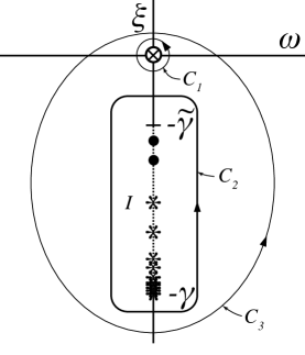
Figure 2: Schematic representation of the poles and zeros of the function $p_{\mathbf{k}}^{\mathrm{TE}}$ in the vicinity of the origin for the Drude model. A zero at the origin is indicated by a cross, while other poles and zeros in the interval $\mathcal{I}$ are shown as black dots and asterisks (interpretation of these symbols in Fig. 3).

Fig. 2 shows a schematic representation of the poles and zeros of the function $p_{\mathbf{k}}^{\mathrm{TE}}$ in the vicinity of the origin for the Drude model. There is one pole due to $C$ and a double zero due to $f_{\mathbf{k}}^{\mathrm{TE}}$, which combine in a zero indicated by the cross at the origin. There then exist a countable infinity of poles and zeros lying in the interval $\mathcal{I}$. Finally, we have to take care of the Matsubara poles which might belong to this interval depending on the respective values of $\gamma$ and $T$. For the case of gold at room temperature, $\xi_{1}$ ($\sim 160$meV) is larger than $\gamma$ ($\sim 35$meV), so that we will consider in the following that there is no Matsubara pole in the interval $\mathcal{I}$. Should this not be the case ($\gamma$ larger than for gold), the Matsubara poles could easily be counted as their positions depend only on $T$, and not on the parameters determining the Foucault poles and zeros.

If the poles in the interval $\mathcal{I}$ were isolated from each other, the functions $p_{\mathbf{k}}^{\mathrm{TE}}$ or $f_{\mathbf{k}}^{\mathrm{TE}}$ would be meromorphic and it would be possible to use Cauchy’s argument principle to obtain information on the number of their poles and zeros. As a matter of fact, the number

$$N\equiv\oint_{\mathcal{C}}\frac{f^{\prime}(z)}{f(z)}\frac{\mathrm{d}z}{2{i}\pi}$$ (18)

would be $N=Z-P$ with $Z$ and $P$ the numbers of zeros and poles of $f$ enclosed in $\mathcal{C}$. In the following, we show how to use an extension of the argument principle to obtain the same kind of information even though the functions $p_{\mathbf{k}}^{\mathrm{TE}}$ or $f_{\mathbf{k}}^{\mathrm{TE}}$ are not meromorphic while the associated $Z$ and $P$ are both infinite.

Numerical evaluations of the number $N$ defined by (18), for the functions $p_{\mathbf{k}}^{\mathrm{TE}}$ and $f_{\mathbf{k}}^{\mathrm{TE}}$ and the contour $\mathcal{C}_{1}$ shown on Fig. 2, confirms the already known fact that $N=1$ for the function $p_{\mathbf{k}}^{\mathrm{TE}}$ on the contour surrounding the origin, with this number being the sum of two zeros for the function $f_{\mathbf{k}}^{\mathrm{TE}}$ and one pole for the function $C$. A new result $N=-2$ is obtained for the contour $\mathcal{C}_{2}$ enclosing the interval $\mathcal{I}$, which means that there are two more poles than zeros there. Finally, for the contour $\mathcal{C}_{3}$ enclosing both the origin and $\mathcal{I}$, we obtain $N=-1$, that is, the sum of results for $\mathcal{C}_{1}$ and $\mathcal{C}_{2}$.

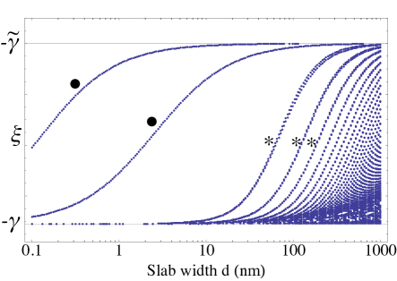
Figure 3: Positions on the imaginary axis of the poles and zeros of the function $p_{\mathbf{k}}^{\mathrm{TE}}$ in the interval $\mathcal{I}$ as a function of the width $d$ of the slabs. Each trajectory marked with a dot follows one single pole whereas each trajectory with an asterisk follows a group of one double zero and two simple poles.

The preceding discussion shows that, even though Cauchy’s argument principle cannot be applied in its common form because $Z$ and $P$ are both infinite, the value of $N=Z-P$ is still well-defined. The same assertion can be understood through a different reasoning, which follows the variation of the poles and zeros when the width $d$ of the slabs is changed. For very thin slabs $d\to 0$, there are essentially two poles whose trajectories as a function of $d$ are marked with dots in Fig. 3. When the value of $d$ is increased, we see the appearance of the infinite number of poles and zeros. Those poles and zeros emerge from the branch point $\xi=-\gamma$ as groups of one zero of order two and two poles of order one, each group marked with an asterisk in Fig. 3. These poles and zeros then fill the whole interval $\mathcal{I}$ when $d\to\infty$. This reasoning explains why we can consider that there are two more Foucault poles than zeros there.

In the limit $\gamma\to 0$, all the poles and zeros converge to the origin, where they collapse into what can be considered as a single pole, according to the discussion just presented in terms of Cauchy’s argument principle. Again these properties will play a key role in the next section for the calculation of the Casimir pressure.

For the sake of completeness, we also discuss the TM case. The function $f_{\mathbf{k}}^{\text{TM}}$ behaves as $z^{0}$ near the origin, and the function $p_{\mathbf{k}}^{\text{TM}}$ has a pole at the origin due to $C$. In the interval $\mathcal{I}$, $p_{\mathbf{k}}^{\text{TM}}$ possesses an equal number of poles and zeros so that we obtain $N=0$ on the contour $\mathcal{C}_{2}$. The result $N=-1$ on the contour $\mathcal{C}_{3}$ is common to both polarizations. The difference in the number of poles and zeros in the interval $\mathcal{I}$ for TE and TM leads to a fundamental difference at the origin in the spectral density $\mathrm{Re}[p_{\mathbf{k}}^{\varsigma}(\omega)]$. These points will be discussed in more detail in the next section.

V The plasma model

We come now to the calculation of the Casimir pressure for mirrors described by the plasma model and, in particular, we carefully discuss the derivation of the Lifshitz-Matsubara sum formula starting from the integral (II) over real frequencies. The application of Cauchy’s residue theorem is much more delicate for $\gamma=0$ than for $\gamma>0$, because the integrand $p_{\mathbf{k}}^{\varsigma}$ has now to be understood in terms of distributions.

We first consider the simplest case of an isolated single pole $z_{m}^{\varsigma}=\omega_{m}^{\varsigma}-{i}\epsilon_{m}^{\varsigma}$ of the function $f_{\mathbf{k}}^{\varsigma}$ corresponding to a propagating Fabry-Perot or plasmonic mode. This single mode lies below the real axis for $\gamma>0$ and comes to touch the real axis with $\epsilon_{m}\to 0$ when $\gamma\to 0$. It is thus clear that the integrand $p_{\mathbf{k}}^{\varsigma}(\omega)$ in (II) contains a Dirac delta distribution associated with this pole. The associated contribution is easily evaluated by applying the so-called Sokhotsky’s formula Vladimirov1971

$$\lim_{\epsilon\rightarrow 0^{+}}\int_{a}^{b}\frac{\varphi(\omega)}{\omega-\omega_{m}\mp{i}\epsilon}\text{d}\omega = \pm i\pi\varphi(\omega_{m})$$

$$+ \mathcal{P}\int_{a}^{b}\frac{\varphi(\omega)}{\omega-\omega_{m}}\text{d}\omega~{}.$$

As the pole is isolated from other ones, we can consider values of $\gamma$ small enough so that the disk $\mathcal{D}_{m}^{\varsigma}$ introduced in (IV) includes a segment $\mathcal{S}_{m}^{\varsigma}$ covering the vicinity of the pole on the real axis. We then apply Sokhotsky’s formula (V) to the function (IV) on this segment to obtain

$$\int_{\mathcal{S}_{m}^{\varsigma}}\frac{\hat{p}_{m}^{\varsigma}(z)}{z-z_{m}^{\varsigma}}\frac{\mathrm{d}\omega}{2\pi}=\mathcal{P}\int_{\mathcal{S}_{m}^{\varsigma}}\frac{\hat{p}_{m}^{\varsigma}(z)}{z-z_{m}^{\varsigma}}\frac{\mathrm{d}\omega}{2\pi}-\frac{{i}}{2}\hat{p}_{m}^{\varsigma}(z_{m}^{\varsigma})~{}.$$ (20)

The real part of the last equation is also

$$\int_{\mathcal{S}_{m}^{\varsigma}}\mathrm{Re}[p_{\mathbf{k}}^{\varsigma}(\omega)]\frac{\mathrm{d}\omega}{2\pi}=\mathcal{P}\int_{\mathcal{S}_{m}^{\varsigma}}\mathrm{Re}[p_{\mathbf{k}}^{\varsigma}(\omega)]\frac{\mathrm{d}\omega}{2\pi}+\frac{1}{2}\mathrm{Im}[\hat{p}_{m}^{\varsigma}(z_{m}^{\varsigma})]~{},$$ (21)

and the last term in (21) is related to the residue (16). This residue is easily seen to be purely imaginary for ordinary as well as evanescent modes.

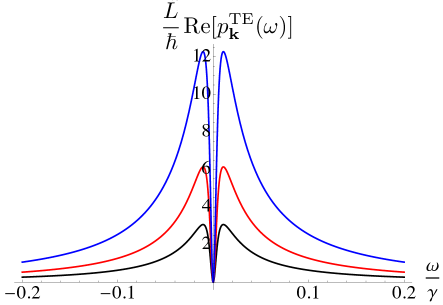
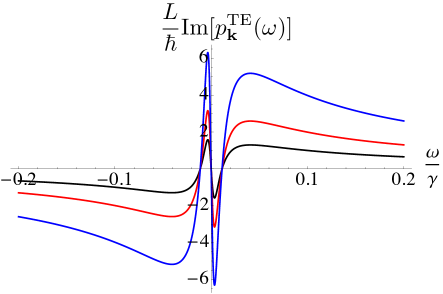
Figure 4: Real (top plot) and imaginary part (bottom plot) of the dimensionless $\frac{L}{\hbar}p_{\mathbf{k}}^{\mathrm{TE}}$ drawn in the vicinity of the origin on the real axis, as a function of the dimensionless parameter $\omega/\gamma$. The curves on each plot with increasing maxima correspond to values of $\gamma$ being 1/4 (blue), 1/2 (red) and 1 (black), respectively, of that of gold. [Colors online]

We then come to the case of modes associated to Foucault current which deserve a specific treatment, as already discussed in section IV. We use the property shown there that all the poles and zeros lying in the vicinity of the origin for the Drude model (see Fig 2) converge in the limit $\gamma\to 0$ to a single pole touching the origin. This idea is confirmed by the drawing in Fig. 4 of the real (top plot) and imaginary (bottom plot) parts of the function $p_{\mathbf{k}}^{\mathrm{TE}}$ as a function of $\omega$ in the vicinity of the origin. For each plot, the bottom curve corresponds to a calculation with the parameters chosen to match gold (with $L=250$ nm), while the middle and top curves correspond to values of $\gamma$ divided respectively by factors 2 and 4.

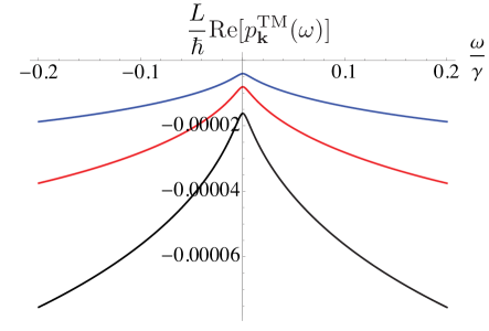
Figure 5: Real part of the dimensionless $\frac{L}{\hbar}p_{\mathbf{k}}^{\mathrm{TM}}$ drawn in the vicinity of the origin on the real axis. Same conventions as for Fig. 4. [Colors online]

The plots on Fig. 4 clearly show that the middle and top curves are identical to the bottom curve multiplied by two and four. As the curves are drawn as a function of the dimensionless quantity $\omega/\gamma$, their integrals tend to a finite limit when $\gamma\to 0$. This scaling property implies that the function $p_{\mathbf{k}}^{\mathrm{TE}}$ has a singularity at the origin, with its real part containing the equivalent of a Dirac delta function $\delta(\omega)$ when $\gamma\to 0$. This Dirac delta function can be treated by Sokhotsky’s formula as in the already discussed case of isolated poles. The situation is clearly different for the TM polarization, as shown by the plots on Fig. 5 (same conventions as for Fig. 4). The function $\mathrm{Re}[p_{\mathbf{k}}^{\mathrm{TM}}]$ tends to 0 when $\gamma\to 0$, so that there is no singularity left at the origin. The difference between TE and TM cases is directly related to the counting of poles and modes in the preceding section.

After this discussion, Sokhotsky’s formula now allows us to write the following relations which are the counterpart of (III) for the plasma model for the contribution to the Casimir pressure for given values of $\mathbf{k}$ and $\varsigma$

$$\int_{-\infty}^{\infty}\mathrm{Re}[p_{\mathbf{k}}^{\varsigma}(\omega)]\frac{\mathrm{d}\omega}{2\pi} = \mathcal{P}\int_{-\infty}^{\infty}\mathrm{Re}[p_{\mathbf{k}}^{\varsigma}(\omega)]\frac{\mathrm{d}\omega}{2\pi}$$ (22)

$$+ \frac{1}{2}\sum_{m}\underset{\omega_{m}^{\varsigma}}{\mathrm{Res}}\left(-{i}p_{\mathbf{k}}^{\varsigma}(z)\right)~{},$$

$$\mathcal{P}\int_{-\infty}^{\infty}\mathrm{Im}[p_{\mathbf{k}}^{\varsigma}(\omega)]\frac{\mathrm{d}\omega}{2\pi} = 0~{}.$$

$\omega_{m}^{\varsigma}$ are the poles on the real axis of $p_{\mathbf{k}}^{\varsigma}$, which come as pairs symmetrically located with respect to the imaginary axis, except for those sitting at the origin. For the TE polarization, the poles are labeled by integers $m\in\mathds{Z}$. The number $m=0$ corresponds to the pole at $\omega_{0}=0$ which collects all the poles and zeros in the vicinity of the origin, as discussed in section IV, while the non-zero integers with opposite signs correspond to poles symmetrically located with respect to the imaginary axis. For the TM polarization, there is no pole of $f_{\mathbf{k}}^{\mathrm{TM}}$ on the imaginary axis, so that the poles are labeled by integers $m\in\mathds{Z}^{\ast}$ (i.e. $m\in\mathds{Z}$ and $m\neq 0$). To repeat, in eq. (22) the Cauchy’s principal value $\mathcal{P}$ is taken at each singularity of the function $\mathrm{Im}[p_{\mathbf{k}}^{\varsigma}(\omega)]$ while the last term originating from the application of Sokhotsky’s formula counts the contributions of Dirac delta distributions in $\mathrm{Re}[p_{\mathbf{k}}^{\varsigma}(\omega)]$.

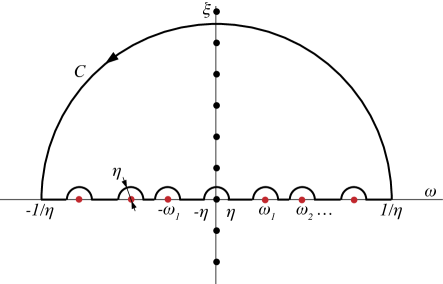
Figure 6: Contour used for the application of Cauchy’s residue theorem for metallic slabs described by the plasma model. The finite number of poles of the function $f_{\mathbf{k}}^{\varsigma}$ are represented as red dots and those due to $C(z)$ by black dots. [Colors online]

As in section III, we now proceed to the derivation of the Lifshitz-Matsubara sum formula by applying Cauchy’s residue theorem to the function $p_{\mathbf{k}}^{\varsigma}(z)$ over the contour shown on Fig. 6, now used for both polarizations. A subtlety arises here, as the branch cut due to $k_{z}$ lying on the real axis for $\omega>c|\mathbf{k}|$ may prevent us to define the punctured disk $\mathcal{D}_{\mathbf{k}}^{\varsigma}$ as previously. A way out of this difficulty is to define a cut with indentations around the poles as was done in Nesterenko2012 . Cauchy’s residue theorem on the contour $\mathcal{C}$ then leads, for both polarizations, to

$$\mathcal{P}\int_{-\infty}^{\infty}p_{\mathbf{k}}^{\varsigma}(\omega)\frac{\mathrm{d}\omega}{2\pi} = \frac{1}{2}\sum_{m\neq 0}\underset{\omega_{m}^{\varsigma}}{\mathrm{Res}}\left({i}p_{\mathbf{k}}^{\varsigma}(z)\right)$$

$$+ \frac{1}{2}\underset{{i}\xi_{0}}{\mathrm{Res}}\left({i}p_{\mathbf{k}}^{\varsigma}(z)\right)+\sum_{n=1}^{\infty}\underset{{i}\xi_{n}^{\varsigma}}{\mathrm{Res}}\left({i}p_{\mathbf{k}}^{\varsigma}(z)\right)~{},$$

where Cauchy’s principal value is again taken at all modes on the real axis, including $\omega_{0}^{\mathrm{TE}}=0$.

Collecting these results with those in (22), we obtain the Casimir pressure between thick metallic slabs described by the plasma model

$$P = -2k_{\mathrm{B}}T\sum_{\mathbf{k}}\left(\sum_{\varsigma}\sum_{n}^{\prime}\kappa_{n}f_{\mathbf{k}}^{\varsigma}({i}\xi_{n})-\frac{1}{2}\kappa_{0}f_{\mathbf{k}}^{\mathrm{TE}}(0)\right)$$ (24)

$$= -2k_{\mathrm{B}}T\sum_{\mathbf{k}}\sum_{\varsigma,n}^{\prime\prime}\kappa_{n}f_{\mathbf{k}}^{\varsigma}({i}\xi_{n})~{},$$

where the primed and double primed sum symbols are respectively defined in (6) and (14). It turns out that (24) has the same form as the final expression (13) obtained for the Drude model in section III. In contrast to the Drude case however, the expression (24) is no longer identical to the commonly used (5). This is obvious in the first line of (24) where the first term matches (5) whereas the last term, comes to cancel the TE contribution at the Matsubara frequency $\xi_{0}$. This cancellation is the main result of the present paper, where it has been deduced through a careful application of Cauchy’s residue theorem to the function $p_{\mathbf{k}}^{\varsigma}$ appearing in the integral expression of the Casimir pressure.

VI Discussion

The Casimir pressure between thick slabs described by a local dielectric function was derived by Lifshitz Lifshitz1956 by using the fluctuations-dissipation theorem Callen1951 and then confirmed by Dzyaloshinskii, Lifshitz and Pitaevskii Dzyaloshinskii1961 . The original derivation by Lifshitz, developed in the spirit of Rytov’s method with fluctuations originating from matter Rytov1953 , is perfectly correct for the case of thick slabs made of dissipative media Polder1971 ; Lifshitz1980 ; Rytov1989 ; Antezza2008 . In such a method, the plasma model can only be considered as the limit $\gamma\to 0$ of the dissipative Drude model.

In the present paper, we have used the derivation of the Casimir pressure as the result of vacuum and thermal radiation pressure on the two mirrors Jaekel1991 . This approach is valid for lossy as well as lossless mirrors Genet2003 ; Lambrecht2006 while reproducing the Lifshitz formula for reflection amplitudes deduced from Fresnel equations (eq.(II) in the present paper). The remark in the preceding paragraph thus has crucial consequences for the derivation of the Lifshitz-Matsubara sum formula (eq. (5.2) in Lifshitz1956 , that is also (5) with the notations of the present paper).

We have confirmed the validity of this formula for dissipative metals as well as dielectrics, for which $r_{\mathbf{k}}^{\mathrm{TE}}(0,k)$ vanishes (eq.(5) is equivalent to eq.(13) in this case). This formula shows the nice property of having a completely symmetrical form for the two polarizations but it also leads to a discontinuity in the calculated thermal Casimir pressure when going from a dissipative model ($\gamma\neq 0$) to a non-dissipative one ($\gamma=0$).

For thick metallic slabs described by the plasma model, we have found the expression (24) for the Casimir pressure, which is not identical to the one commonly used (5). This follows from the fact that the Matsubara pole for the TE mode at $\xi_{0}$ does not contribute for a lossless plasma metal, in spite of a non-vanishing value of $r_{\mathbf{k}}^{\mathrm{TE}}(0,k)$. As a consequence, the discontinuity in the calculated thermal Casimir pressure between dissipative and non-dissipative metals disappears. It has however to be acknowledged that this result does not solve the discrepancy observed between theory and some experiments Klimchitskaya2006 ; Brevik2006 ; Lambrecht2011 .

The interpretation of this result is that the contribution to the pressure corresponding to the non-vanishing value of $r_{\mathbf{k}}^{\mathrm{TE}}(0,k)$ is canceled by an additional contribution originating from the collapse of all poles due to the Foucault modes at the origin of the complex plane. This has been proven by two different but equivalent approaches, first by counting the poles and zeros of the causal function $p_{\mathbf{k}}^{\mathrm{TE}}$ (§ IV), and then by examining the behavior in the vicinity of the origin of the density $\mathrm{Re}[p_{\mathbf{k}}^{\mathrm{TE}}]$ (§ V). We have shown in the present paper that this contribution of Foucault modes, usually ignored in calculations of the Casimir pressure for a lossless plasma model, leaves a finite contribution in the limit $\gamma\to 0$, which is just the difference between the common form of the Lifshitz-Matsubara sum formula and its corrected expression.

- (1) H.B.G. Casimir, Proc. K. Ned. Akad. Wet. (Phys.) 51 79 (1948).
- (2) K.A. Milton, The Casimir effect, physical manifestation of zero-point energy (World Scientific, 2001).
- (3) G.L. Klimchitskaya, U. Mohideen and V.M. Mostepanenko, Rev. Mod. Phys. 81 1827 (2009).
- (4) S. Lamoreaux, in Casimir physics, eds. D.A.R. Dalvit et al, Lecture Notes in Physics 834 (Springer-Verlag, 2011) p.219.
- (5) F. Capasso, J.N. Munday, and H.B. Chan, in Casimir physics, eds. D.A.R. Dalvit et al, Lecture Notes in Physics 834 (Springer-Verlag, 2011) p.249.
- (6) R. Decca, V. Aksyuk, and D. López, in Casimir physics, eds. D.A.R. Dalvit et al, Lecture Notes in Physics 834 (Springer-Verlag, 2011) p.287.
- (7) G.L. Klimchitskaya and V.M. Mostepanenko, Contemp. Phys. 47 131 (2006).
- (8) I. Brevik, S.Å. Ellingsen and K. Milton, New J. Phys. 8 236 (2006).
- (9) A. Lambrecht, A. Canaguier-Durand, R. Guérout and S. Reynaud, in Casimir physics, eds. D.A.R. Dalvit et al, Lecture Notes in Physics 834 (Springer-Verlag, 2011) p.97.
- (10) E.M Lifshitz, Sov. Phys. JETP 2 73 (1956).
- (11) I.E. Dzyaloshinskii, E.M. Lifshitz and L.P. Pitaevskii, Sov. Phys. Uspekhi 4 153 (1961).
- (12) M.-T. Jaekel and S. Reynaud, J. Physique I 1 1395 (1991).
- (13) A. Lambrecht and S. Reynaud, Euro. Phys. J. D 8 309 (2000).
- (14) V.B. Svetovoy, P.J. van Zwol, G. Palasantzas and J.Th.M. De Hosson, Phys. Rev. B 77 035439 (2008).
- (15) M. Boström and B.E. Sernelius, Phys. Rev. Lett. 84 4757 (2000).
- (16) G.-L. Ingold, A. Lambrecht and S. Reynaud, Phys. Rev. E 80 041113 (2009).
- (17) I. Brevik and J.S. Høye, Eur. J. Phys. 35 015012 (2014).
- (18) R.S. Decca, D. López, E. Fischbach et al, Phys. Rev. D 75 077101 (2007).
- (19) R.S. Decca, D. López, E. Fischbach et al, Eur. Phys. J. C 51 963 (2007).
- (20) C.-C. Chang, A. A. Banishev, R. Castillo-Garza et al, Phys. Rev. B 85 165443 (2012).
- (21) A.O. Sushkov, W.J. Kim, D.A.R. Dalvit and S.K. Lamoreaux, Nature Physics 7 230 (2011).
- (22) K. Milton, Nature Physics 7 190 (2011).
- (23) W.J. Kim, A.O. Sushkov, D.A.R. Dalvit and S.K. Lamoreaux, Phys. Rev. A 81 022505 (2010).
- (24) S. Reynaud and A. Lambrecht, in Quantum Optics and Nanophotonics to appear (Oxford University Press, 2014).
- (25) M. Bordag, Eur. Phys. J. C 71 1788 (2011).
- (26) T. Matsubara, Prog. Theor. Phys. 14 351 (1955).
- (27) A.A. Banishev, C.-C. Chang, G. L. Klimchitskaya, V.M. Mostepanenko and U. Mohideen, Phys. Rev. B 85 195422 (2012).
- (28) A.A. Banishev, G.L. Klimchitskaya, V.M. Mostepanenko and U. Mohideen, Phys. Rev. B 88 155410 (2013).
- (29) R.O. Behunin, F. Intravaia, D.A.R. Dalvit, P.A. Maia Neto and S. Reynaud, Phys. Rev. A 85 012504 (2012).
- (30) W. Broer, G. Palasantzas, J. Knoester and V.B. Svetovoy, Phys. Rev. B 85 155410 (2012).
- (31) C. Genet, A. Lambrecht and S. Reynaud, Phys. Rev. A 67 043811 (2003).
- (32) A. Lambrecht, P.A. Maia Neto and S. Reynaud, New J. Phys. 8 243 (2006).
- (33) J. Schwinger, L.L. DeRaad, Jr. and K.A. Milton, Ann. Phys. 115 1 (1978).
- (34) F. Intravaia and A. Lambrecht, Phys. Rev. Lett. 94 110404 (2005).
- (35) F. Intravaia, C. Henkel and A. Lambrecht, Phys. Rev. A 76 033820 (2007).
- (36) F. Intravaia and C. Henkel, Phys. Rev. Lett. 103 130405 (2009).
- (37) F. Intravaia, S.Å. Ellingsen and C. Henkel, Phys. Rev. A 82 032504 (2010).
- (38) V. S. Vladimirov, Equations of Mathematical Physics, (Decker New York, 1971).
- (39) V. Nesterenko and I. Pirozhenko, Phys. Rev. A 86 052503 (2012).
- (40) H.B. Callen and T.A. Welton, Phys. Rev. 83 34 (1951).
- (41) S.M. Rytov, Theory of Electric Fluctuations and Thermal Radiation (The Academy of Sciences, Moscow, 1953).
- (42) D. Polder and M. Van Hove, Phys. Rev. B 4 3303 (1971).
- (43) E.M. Lifshitz and L.P. Pitaevskii, L.D. Landau and E.M. Lifshitz Course of Theoretical Physics, Statistical Physics Part 2 §77 (1980).
- (44) S.M. Rytov, Y.A. Kravtsov and V.I. Tatarskii, Principles of Statistical Radiophysics (Springer, 1989).
- (45) M. Antezza, L.P. Pitaevskii, S. Stringari, and V.B. Svetovoy, Phys. Rev. A 77 022901 (2008).