Maximum mass of stable magnetized highly super-Chandrasekhar white dwarfs: stable solutions with varying magnetic fields

Abstract

We address the issue of stability of recently proposed significantly super-Chandrasekhar white dwarfs. We present stable solutions of magnetostatic equilibrium models for super-Chandrasekhar white dwarfs pertaining to various magnetic field profiles. This has been obtained by self-consistently including the effects of the magnetic pressure gradient and total magnetic density in a general relativistic framework. We estimate that the maximum stable mass of magnetized white dwarfs could be more than $3$ solar mass. This is very useful to explain peculiar, overluminous type Ia supernovae which do not conform to the traditional Chandrasekhar mass-limit.

1 Introduction

Type Ia supernovae are one of the most widely studied astronomical events and rightfully so because of their enormous importance in measuring cosmic distances. Although not everything is understood about these events, the general consensus is that they are produced due to the thermonuclear explosion of a white dwarf having mass very close to the Chandrasekhar limit of $1.44M_{\odot}$, when $M_{\odot}$ being the mass of Sun [1]. However, recent observations of a fast-growing number of several peculiar, overluminous type Ia supernovae, e.g. SN 2006gz, SN 2007if, SN 2009dc, SN 2003fg, bring even this basic idea into serious question, as they are best explained by invoking progenitor white dwarfs with super-Chandrasekhar mass in the range $2.1-2.8M_{\odot}$ [2, 3, 4, 5, 6, 7].

In our previous works [8, 9, 10, 11, 12, 13, 14], we addressed this issue and showed that strongly magnetized white dwarfs can violate the sacrosanct Chandrasekhar limit significantly, thus solving the puzzle posed by these peculiar supernovae. We essentially modeled the central region of the white dwarf having a strong constant magnetic field $B$, which would fall off near the surface. However, a few authors [15, 16] have questioned the stability of our super-Chandrasekhar white dwarfs, to which we have partially responded in our latest work [14] and which we address more rigorously and quantitatively in the current work. On the other hand, Federbush et al. [17] have carried out an extensive mathematical analysis of stable magnetic star solutions including the polytrope describing our super-Chandrasekhar white dwarfs [11]. They have proved that such a polytrope will remain stable, provided the underlying magnetic field profile is constrained appropriately.

We take this opportunity to point out that one of the authors, Dong et al. [15], have argued completely erroneously that our model of super-Chandrasekhar white dwarfs would lead to an unphysical large mass, if the contribution of magnetic density, $\rho_{B}=B^{2}/(8\pi c^{2})$, is included. They have incorrectly calculated a value of $24M_{\odot}$ as the contribution of $\rho_{B}$ to the total mass of the particular white dwarf having central magnetic field $B_{\rm cent}=8.8\times 10^{17}$ G, radius $R=70$ km and mass $M=2.58M_{\odot}$ (computed without $\rho_{B}$) [11]. If, following Dong et al., we indeed consider a constant $B$ throughout the above white dwarf, then to arrive at the $M$ and $R$ correctly in the Newtonian framework, one must solve the following set of equations simultaneously (when magnetic pressure gradient $dP_{B}/dr=0$ and magnetic tension $\vec{B}.\nabla\vec{B}|_{r}=0$, as chosen by Dong et al. and us previously):

$$\frac{dP(r)}{dr}+\frac{dP_{B}}{dr}=-\frac{GM(r)}{r^{2}}(\rho(r)+\rho_{B})+\frac{\vec{B}\cdot\nabla\vec{B}|_{r}}{4\pi},\,\,\,\,\frac{dM(r)}{dr}=4\pi r^{2}(\rho(r)+\rho_{B}),$$ (1.1)

where $r$ is the radial distance from the center of the white dwarf, $P$ the matter pressure, $P_{B}$ the magnetic pressure, $\rho$ the matter density and $G$ Newton’s gravitation constant. Mistake of Dong et al was not considering $\rho_{B}$ in the first equation but considering only in the second equation above. A self-consistent inclusion of $\rho_{B}$, however, shows that both $M$ and $R$ of the white dwarf decrease drastically, due to the increased gravitational force because of the increased total density (see Figure 1 and §5 of [14]). When $B$ decreases away from the center, one must additionally account for the effects of $dP_{B}/dr$ (and $\vec{B}.\nabla\vec{B}|_{r}$), which will lead to an increase of $M$ and $R$, as done in the current work. The point to be emphasized is that if one wants to include the effects of $P_{B}$ and $\rho_{B}$ self-consistently, then they have to be included in both the equations above, which unfortunately Dong et al. did not do. To avoid complicacy, we, earlier, did not include these effects in either of the equations. We shall show here that our earlier solutions [11] are much closer to the exact results compared to that obtained by Dong et al [15].

In this work, we present stable, magnetostatic equilibrium solutions of significantly super-Chandrasekhar white dwarfs in the framework of general relativity, obtained by self-consistently including the effects of the pressure gradient due to a varying $B$ and also $\rho_{B}$. Note that a general relativistic approach is important in order to accurately understand the effects of $\rho_{B}$ and $P_{B}$ for the high density and high $B$ white dwarfs. The current work firmly corroborates the existence of our super-Chandrasekhar white dwarfs.

In the next section, we discuss the constraints imposed on the magnetic field profiles along with the equations to be solved. Subsequently, we describe various solutions of super-Chandrasekhar white dwarfs in section 3. Finally, we end with conclusions in section 4.

2 Magnetic field profiles and basic equations

Since magnetized white dwarfs form the basis of our work, it is important to note that a large number of them have been discovered by the Sloan Digital Sky Survey (SDSS), having high surface fields $10^{5}-10^{9}$G [18, 19]. It is likely that the observed surface field is several orders of magnitude smaller than the central field. Thus, it is important to perform numerical calculations, in the presence of a varying $B$, to self-consistently account for $dP_{B}/dr$ and $\rho_{B}$, in addition to $dP/dr$. Keeping this in mind, we model the variation of $B$ as a function of $\rho$ inside the white dwarf by adopting the profile proposed by Bandyopadhyay et al. [20]. This is very commonly applied to magnetized neutron stars (see, e.g., [21]) given by

$$B\left(\frac{\rho}{\rho_{0}}\right)=B_{s}+B_{0}\left[1-\exp\left(-\eta\left(\frac{\rho}{\rho_{0}}\right)^{\gamma}\right)\right],$$ (2.1)

where $\rho_{0}$, for the present purpose, is chosen to be one-tenth of the central matter density ($\rho_{c}$) of the corresponding white dwarf, $B_{s}$ is the surface magnetic field, $B_{0}$ is a parameter having dimension of $B$, $\eta$ and $\gamma$ are dimensionless parameters which determine how exactly the field decays from the center to the surface. Note that as $\rho\rightarrow 0$ close to the surface of the white dwarf, $B\rightarrow B_{s}$.

In this work, we present the cases with $10^{9}$ G $\leq B_{s}\leq 10^{12}$ G. Note that the lower limit for $B_{s}$ is guided by the aforementioned SDSS observations. However, for $B_{\rm cent}\geq 10^{14}$ G, what we will consider in this work, the result is independent of $B_{s}$ chosen above. Now, it has already been shown in our previous works [9, 11] that for $B>B_{cr}=4.414\times 10^{13}$ G, the effect of Landau quantization becomes important which modifies the equation of state (EoS) of the electron degenerate matter constituting the white dwarf and gives rise to super-Chandrasekhar white dwarfs. Hence, in this work we consider different values of $B_{0}$ such that the resulting $B_{\rm cent}$ of the white dwarf is super-critical, i.e. $B_{\rm cent}>B_{cr}$. We recall that the maximum number of Landau levels ($\nu_{m}$) occupied by the electrons is given by [9]

$$\nu_{m}=\frac{\left(\frac{E_{Fmax}}{m_{e}c^{2}}\right)^{2}-1}{2B/B_{cr}},$$ (2.2)

where $E_{Fmax}$ is the maximum Fermi energy of the system, $m_{e}$ the mass of the electron and $c$ the speed of light. Thus, for a fixed $E_{Fmax}$, as $B$ decreases from the center to the surface of the white dwarf, $\nu_{m}$ increases. Consequently, the underlying EoS is constructed taking this variation of $B$ into account, such that near the center of the white dwarf, it is (strongly) Landau quantized (see, e.g., [9]), while away from the center it approaches Chandrasekhar’s EoS [1].

Now, it is known that in the presence of a strong $B$, the total pressure of the system may become anisotropic [21], such that it is in the direction perpendicular to $B$ given by $P_{\perp}=P+B^{2}/(8\pi)$ (neglecting magnetization, which is much smaller compared to $B^{2}/(8\pi)$ for the $B$ of present interest), while that in the direction parallel to $B$ is given by $P_{||}=P-B^{2}/(8\pi)$. If $B$ becomes too large, then one notices that $P_{||}$ may vanish (and maybe even negative) and this might lead to instabilities in the system. For the present purpose, however, we model our white dwarfs with varying $B$, by adopting the same magnetostatic balance equation as in general relativity, well known as the (magnetized) Tolman-Oppenheimer-Volkoff (TOV) equation [22] (which is applicable for compact objects having an overall isotropic pressure), using isotropic magnetic pressure to be $P_{B}=B^{2}/(24\pi)$. Validity of such a consideration has been already justified earlier [23, 14, 24, 25, 26]. In particular, Cheoun et al. [24] invoked randomly oriented magnetic domains, where the random currents cancel each other, to justify the spherically symmetric magnetic field configuration of the strongly magnetized neutron stars. This corresponds to force free fields in the domain forming region. On the other hand, Herrera & Barreto [26] invoked a general formalism to describe general relativistic polytropes for anisotropic matter, showing the possibility of two different polytropic EoSs. The present work can be treated as an application of this formalism, when the density of the polytropic EoS consists only of the matter density (their Case I) such that $P=K\rho^{1+1/n}$, corresponding to a particular case of the polytropes, where $n$ is the polytropic index and $K$ the polytropic constant. Furthermore, the white dwarfs in the current work are the polytropes for anisotropic fluids described by Herrera & Barreto [26], with appropriate modification of the anisotropic contribution appearing in their Eq. (53) by the magnetic pressure and density. Although they noted that spherical symmetry can be broken in the presence of a very strong magnetic field, when magnetized Fermi fluids may be regarded as anisotropic systems, the choice of spherical white dwarfs in the present work, however, is not expected to change the main conclusions. Hence, the set of equations we solve are

$$\frac{dM(r)}{dr}=4\pi r^{2}(\rho(r)+\rho_{B}),$$ (2.3)

$$\frac{d\rho(r)}{dr}=-\frac{G\left(\rho(r)+\rho_{B}+\frac{(P(r)+P_{B})}{c^{2}}\right)\left(M(r)+\frac{4\pi r^{3}(P(r)+P_{B})}{c^{2}}\right)}{r^{2}\left(1-\frac{2GM(r)}{c^{2}r}\right)\left(\frac{dP(r)}{d\rho}+\frac{dP_{B}}{d\rho}\right)}.$$ (2.4)

Keeping the above consideration of a possible instability due to anisotropic pressure in mind, we propose two plausible constraints on the magnetic field profile in this work, such that: (i) the average parallel pressure, given by $P-P_{B}$, should remain positive throughout the white dwarf, (ii) the parallel pressure given by $P_{||}$ should remain positive throughout the white dwarf (note that (ii) automatically guarantees (i) as well). The two constraints have been illustrated in Figure 1 with an example. Note that an attempt to model magnetized, significantly super-Chandrasekhar white dwarfs was made earlier in the Newtonian framework, however, without imposing realistic constraints on the field [23].

Figure 1(a) represents constraint (i) for a given EoS. Here, $B_{\rm cent}=4.4\times 10^{14}$ G, $E_{Fmax}=20m_{e}c^{2}$, the number of occupied Landau levels at the center $\nu_{mc}=20$ (as calculated from Eq. (2.2)), $\gamma=0.9$ and $\eta=0.843$. Note that Figure 1(a) represents a limiting magnetic profile, such that $P_{B}$ is just equal to $P$ at some point inside the white dwarf. For a fixed $\gamma$, if one varies $\eta$, then one obtains such a limiting profile for a maximum value of $\eta=\eta_{max}$. Only for $\eta<\eta_{max}$, $P_{B}<P$ throughout. Similarly, Figure 1(b) represents constraint (ii) for $B_{\rm cent}=4.22\times 10^{14}$ G, $E_{Fmax}=20m_{e}c^{2}$, $\nu_{mc}=21$, $\gamma=0.9$ and $\eta_{max}=0.403$. Note that the significance of the limiting cases shown in Figures 1(a) and (b) lie in the fact that they correspond to the maximum stable mass of the white dwarf in each case, in the presence of a varying $B$, as we shall see next.

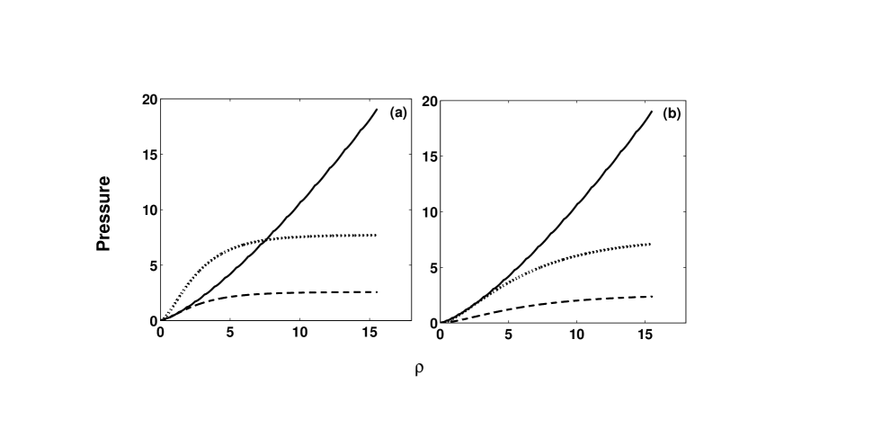
Figure 1: Various pressures as functions of $\rho$ — (a) $P\geq B^{2}/(24\pi)$ throughout (constraint (i)). (b) $P\geq B^{2}/(8\pi)$ throughout (constraint (ii)). The solid, dotted and dashed lines represent $P$, $B^{2}/(8\pi)$ and $B^{2}/(24\pi)$ respectively. Pressure is in units of $10^{27}$ ergs/cc and $\rho$ in units of $10^{9}$ gm/cc.

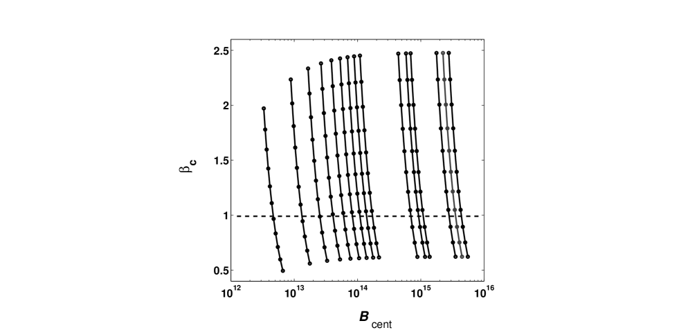
Figure 2: Plasma-$\beta_{c}$ as a function of $B_{\rm cent}$ for various EoSs — from left to right each solid line corresponds to $E_{Fmax}=2,3,4,5,6,7,8,9,10,20,23,25,40,45$ and $50m_{e}c^{2}$ respectively. The filled circles on each solid line correspond to, from top to bottom, $\nu_{mc}=20,19,18,17,16,15,14,13,12,11$ and $10$ respectively. $B_{\rm cent}$ is in units of G.

3 Solutions of super-Chandrasekhar white dwarfs

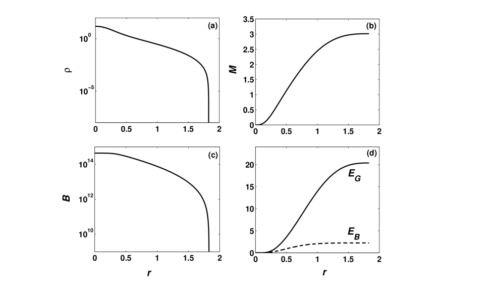
Figure 3: Solutions of a super-Chandrasekhar white dwarf having EoS corresponding to Figure 1(a). (a) $\rho$, (b) $M$, (c) $B$, as functions of $r$ within the white dwarf. (d) $E_{G}$ and $E_{B}$ as functions of $r$. $M$, $\rho$, $r$ and $B$ are in units of $M_{\odot}$, $10^{9}$ gm/cc, 1000 km and G respectively, while $E_{G}$ and $E_{B}$ are in units of $10^{51}$ ergs.

With the magnetic profiles set according to the above constraints, we now solve Eqs. (2.3) and (2.4) subjected to the boundary conditions $\rho(0)=\rho_{c}$ and $M(0)=0$. As an additional criterion for stability, independent of constraints (i) and (ii), $\rho_{c}$ is chosen such that the plasma-$\beta$ at the center, $\beta_{c}=P_{c}/(B_{\rm cent}^{2}/8\pi)>1$ (i.e., central $P_{||}>0$) always, where $P_{c}$ is the central matter pressure. If $P_{c}$ is the maximum possible pressure for a given EoS, which is determined by the choice of $E_{Fmax}$ and $\nu_{mc}$ (see Eq. (17) of [9] for the expression of $P$ for a Landau quantized system), then we arrive at a very interesting result as illustrated in Figure 2. In Figure 2, we compute $\beta_{c}$ for different combinations of $E_{Fmax}$ and $\nu_{mc}$, such that only the region above the $\beta_{c}=1$ line is allowed as per our condition. One observes that as $E_{Fmax}$ increases from 2 to $6m_{e}c^{2}$, the minimum allowed value of $\nu_{mc}$, for which $\beta_{c}\geq 1$ just, decreases from 15 to 13. However, for $E_{Fmax}\gtrsim 6m_{e}c^{2}$, the minimum allowed value of $\nu_{mc}$ saturates at $13$, i.e., $\beta_{c}>1$ is satisfied for all $B_{\rm cent}$ having $\nu_{mc}\geq 13$. This additionally constrains the maximum possible $B_{\rm cent}$ for a given $E_{Fmax}$, which also corresponds to the maximum stable mass of the white dwarf.

Figure 3 depicts the solutions of Eqs. (2.3) and (2.4) for a single white dwarf, having $\rho_{c}=1.55\times 10^{10}$ gm/cc and $B_{\rm cent}=4.4\times 10^{14}$ G, whose EoS and necessary magnetic field constraints are portrayed in Figure 1(a). Figures 3(a), (b) and (c) show the variations of $\rho$, $M$ and $B$ respectively inside the white dwarf. The resulting white dwarf is clearly highly super-Chandrasekhar, having $M=3.01M_{\odot}$ and $R=1828$ km. Figure 3(d) shows the variations of the gravitational energy $E_{G}$ and the magnetic energy $E_{B}$ inside the white dwarf. The total gravitational energy of the white dwarf is given by $E_{GT}=\int_{0}^{R}\phi~{}dM$, where $\phi$ is the gravitational potential in general relativity including magnetic effects, while the total magnetic energy of the white dwarf is given by $E_{BT}=\int_{0}^{R}P_{B}~{}d^{3}r$. Very importantly, we observe that for this white dwarf, $E_{GT}=2.035\times 10^{52}$ ergs, which is almost an order of magnitude larger than $E_{BT}=2.246\times 10^{51}$ ergs, thus firmly establishing it as stable.

Various results obtained by considering different magnetic field profiles, $\nu_{mc}$ and $E_{Fmax}$, are summarized in Figure 4. We further restrict $E_{Fmax}$ to $50m_{e}c^{2}$, in order to avoid possible neutronization of the matter. Figure 4(a) shows the variation of $M$ with $\gamma$ for a fixed $E_{Fmax}$ and $B_{\rm cent}$. We note that as $\gamma$ increases, $M$ also increases, until $\gamma=0.9$ for constraint (i) and $\gamma=0.8$ for constraint (ii), after which $M$ starts decreasing again. The maximum mass ($M_{max}$) for constraint (i) is $3.33M_{\odot}$ while that for constraint (ii) is $2.05M_{\odot}$.

Figure 4(b) shows the variation of $M$ with $E_{Fmax}$ for a fixed $B_{\rm cent}$ and $\gamma$. Since we are interested in the maximum possible mass of the white dwarf, we fix $\gamma$ accordingly. We note that as $E_{Fmax}$ increases, $M$ attains a peak and then decreases very slightly. For constraint (i) $M_{max}=3.33M_{\odot}$ at $E_{Fmax}\sim 21m_{e}c^{2}$, while for constraint (ii) $M_{max}=2.05M_{\odot}$ at $E_{Fmax}\sim 25m_{e}c^{2}$.

Figure 4(c) shows the variation of $M$ with $\nu_{mc}$ for a fixed $E_{Fmax}$ and $\gamma$. We observe that with the decrease in $\nu_{mc}$ or a corresponding increase in $B_{\rm cent}$, $M$ increases, as was also shown in our previous works [9, 11]. For constraint (i) $M_{max}=3.33M_{\odot}$, while for constraint (ii) $M_{max}=2.1M_{\odot}$, both at $B_{\rm cent}=6.77\times 10^{14}$ G (or $\nu_{mc}=13$).

Finally, Figure 4(d) shows the mass-radius relations for the cases in Figure 4(c) along with the corresponding cases with $E_{Fmax}=50m_{e}c^{2}$. We observe that for both constraints (i) and (ii), $R$ decreases as $M$ increases, i.e. a stronger magnetic field makes the star more compact (as argued previously, see, e.g., [9, 11]). Additionally, we note that the radii of the white dwarfs having $E_{Fmax}=50m_{e}c^{2}$ are more than a factor of two smaller than those with $E_{Fmax}=20m_{e}c^{2}$ for roughly the same range of $M$. This is expected because a higher $E_{Fmax}$ implies a higher $\rho_{c}$ and hence more compact objects. For example, for the cases pertaining to constraint (i), $M_{max}=3.33M_{\odot}$ and $R=1605$ km for $E_{Fmax}=20m_{e}c^{2}$ ($\rho_{c}=1.55\times 10^{10}$ gm/cc), while $M_{max}=3.28M_{\odot}$ and $R=670$ km for $E_{Fmax}=50m_{e}c^{2}$ ($\rho_{c}=2.42\times 10^{11}$ gm/cc). Similarly, for the cases pertaining to constraint (ii), $M_{max}=2.1M_{\odot}$ and $R=1237$ km for $E_{Fmax}=20m_{e}c^{2}$, while $M_{max}=2.06M_{\odot}$ and $R=512$ km for $E_{Fmax}=50m_{e}c^{2}$.

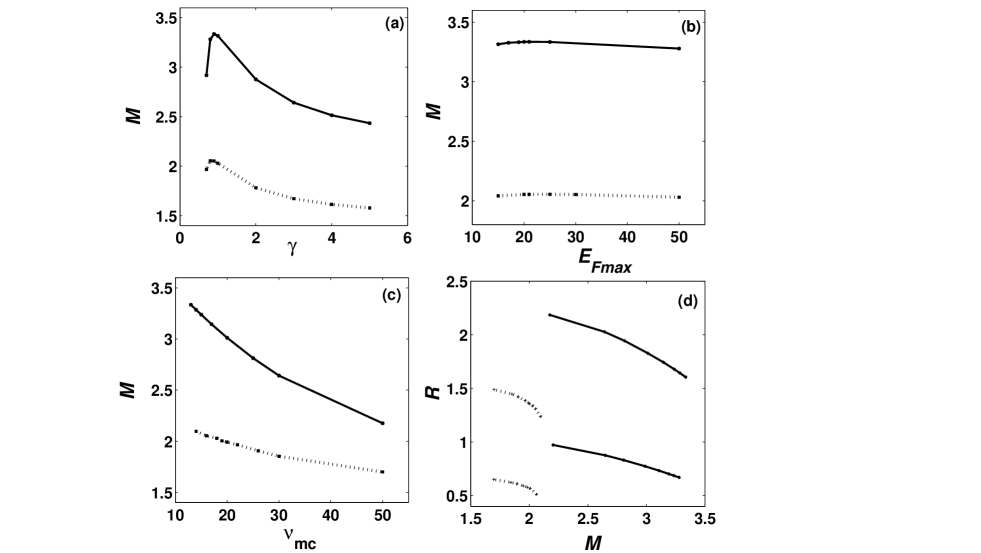
Figure 4: Super-Chandrasekhar white dwarfs with varying $B$ — The solid and dotted lines represent the cases corresponding to constraints (i) and (ii) respectively (see text). (a) $M$ as a function of $\gamma$ for $E_{Fmax}=20m_{e}c^{2}$, $B_{\rm cent}=6.77\times 10^{14}$ G, $\eta=\eta_{max}$ for respective $\gamma$s. (b) $M$ as a function of $E_{Fmax}$ for $B_{\rm cent}=6.77\times 10^{14}$ G, $\gamma=0.9$ for solid line and $B_{\rm cent}=5.18\times 10^{14}$ G, $\gamma=0.8$ for dotted line. (c) $M$ as a function of $\nu_{mc}$ for $E_{Fmax}=20m_{e}c^{2}$, $\gamma=0.9$ for solid line and $\gamma=0.8$ for dotted line. (d) The topmost solid and dotted lines represent the $M$-$R$ relations corresponding to (c), while the solid and dotted lines at the bottom represent the $M$-$R$ relations corresponding to (c) but with $E_{Fmax}=50m_{e}c^{2}$. $M$, $R$ and $E_{Fmax}$ are in units of $M_{\odot}$, 1000 km and $m_{e}c^{2}$ respectively.

In order to confirm the stability of these super-Chandrasekhar white dwarfs, we resort to Table 1, which describes the properties of some of the super-Chandrasekhar white dwarfs having $E_{Fmax}=20m_{e}c^{2}$ shown in Figure 4(d). The seven columns represent respectively: the constraint conditions (i) or (ii) on the magnetic profile; $M$; $R$; $E_{GT}$; $E_{BT}$; the equipartition magnetic field $B_{\rm equi}$ as defined in §2 of [14] (with polytropic index $n\approx 3$, as is true on average for the EoSs of the cases described in Table 1); and the average magnetic field, $B_{\rm avg}=\frac{1}{R}\int_{0}^{R}B(\rho(r))~{}dr$, of the white dwarf. It is evident from Table 1 that for all the cases, $E_{GT}$ significantly dominates over $E_{BT}$, which assures the stability of any magnetized compact object. Although $B_{\rm equi}$ is only a rough estimate, we still note that $B_{\rm avg}$ in all the cases is substantially less than $B_{\rm equi}$, thus ensuring that the corresponding super-Chandrasekhar white dwarfs are highly stable.

4 Conclusions

Constraint	$M$ ($M_{\odot}$)	$R$ (1000 km)	$E_{GT}$ ($10^{51}$ ergs)	$E_{BT}$ ($10^{51}$ ergs)	$B_{\rm equi}$ ($10^{14}$ G)	$B_{\rm avg}$ ($10^{14}$ G)
	2.17	2.18	12.75	0.77	1.22	0.72
(i) $P\geq B^{2}/(24\pi)$	2.64	2.03	17.01	1.46	1.72	1.13
	3.33	1.60	23.41	3.22	3.47	2.41
	1.70	1.49	7.99	0.30	2.06	0.76
(ii) $P\geq B^{2}/(8\pi)$	1.96	1.38	9.94	0.67	2.74	1.41
	2.10	1.24	10.88	0.93	3.67	2.04

Table 1: Properties of super-Chandrasekhar white dwarfs with $E_{Fmax}=20m_{e}c^{2}$ in Figure 4(d).

We have reestablished the existence of stable, significantly super-Chandrasekhar white dwarfs by considering different, varying magnetic field profiles in a general relativistic framework, subjected to certain constraints to ensure stability. The maximum mass of the white dwarf can be as large as $3.33M_{\odot}$, depending on the underlying nature of the variation of $B$ with $\rho$. Note that a violation of the constraints on the magnetic field profile leads to unphysical white dwarfs. For example, for the case shown in Figure 1(a), if $\eta$ is chosen to be 3.5, which violates constraint (i), we obtain an unusually massive white dwarf having $M=28.4M_{\odot}$ and $R=6880$ km (note that even relatively smaller mass white dwarfs also could be unphysical if constraint (i) is violated).

For all the cases described in this work, $E_{GT}\gg E_{BT}$ and also $B_{\rm equi}>B_{\rm avg}$, which show that these magnetized super-Chandrasekhar white dwarfs are highly bound systems. We note that the same calculations, when carried out in a Newtonian framework, also yield stable white dwarfs, but with a slightly higher $M$ and $R$ for each of the cases discussed here.

Note that in our previous works [9, 11], we carried out spherically symmetric calculations in the Newtonian framework, by assuming that the field is constant in a large central region. Let us now assume a very slowly varying field according to Eq. (2.1), such that $B_{s}=8.76\times 10^{15}$ G, $B_{\rm cent}=8.8\times 10^{15}$ G, $\gamma=0.47$ and $\eta=0.00178$ for $E_{Fmax}=20m_{e}c^{2}$. If we repeat the same calculation in the Newtonian framework by including the corresponding $\rho_{B}$ and $dP_{B}/dr$ in the magnetostatic balance and mass equations appropriately, we arrive at $M=2.44M_{\odot}$ and $R=570$ km, practically the same as what we have already reported [9, 11]. Such a super-Chandrasekhar white dwarf would have almost zero $dP_{B}/dr$ compared to $dP/dr$ and hence would be stable. Interestingly, neutron stars under magnetar models with $B_{s}\sim 10^{15}$ G are also generally believed to have little difference between the magnetic fields at center and surface, when the superconducting effect could not allow a large $B_{\rm cent}$, making $dP_{B}/dr$ very small. This is analogous to the aforementioned example of super-Chandrasekhar white dwarfs and, hence, they could be excellent candidates for soft gamma-ray repeaters (SGRs) and anomalous X-ray pulsars (AXPs). Nevertheless, the other stable super-Chandrasekhar white dwarfs, having a smaller $B_{s}$, can also adequately explain SGR/AXP phenomena [27].

References

- [1] S. Chandrasekhar, The highly collapsed configurations of a stellar mass (Second paper), Mon. Not. R. Astron. Soc. 95 (1935) 207.
- [2] D. A. Howell et al., The type Ia supernova SNLS-03D3bb from a super-Chandrasekhar-mass white dwarf star, Nature 443 (2006) 308 [astro-ph/0609616].
- [3] R. A. Scalzo et al., Nearby supernova factory observations of SN 2007if: First total mass measurement of a super-Chandrasekhar-mass progenitor, Astrophys. J. 713 (2010) 1073 [arXiv:1003.2217].
- [4] M. Hicken et al., The luminous and carbon-rich supernova 2006gz: A double degenerate merger?, Astrophys. J. 669 (2007) L17 [arXiv:0709.1501].
- [5] M. Yamanaka et al., Early phase observations of extremely luminous type Ia supernova 2009dc, Astrophys. J. 707 (2009) L118 [arXiv:0908.2059].
- [6] J. M. Silverman et al., Fourteen months of observations of the possible super-Chandrasekhar mass type Ia supernova 2009dc, Mon. Not. R. Astron. Soc. 410 (2011) 585 [arXiv:1003.2417].
- [7] S. Taubenberger et al., High luminosity, slow ejecta and persistent carbon lines: SN 2009dc challenges thermonuclear explosion scenarios, Mon. Not. R. Astron. Soc. 412 (2011) 2735 [arXiv:1011.5665].
- [8] A. Kundu and B. Mukhopadhyay, Mass of highly magnetized white dwarfs exceeding the Chandrasekhar limit: An analytical view, Mod. Phys. Lett. A 27 (2012) 1250084 [arXiv:1204.1463].
- [9] U. Das and B. Mukhopadhyay, Strongly magnetized cold degenerate electron gas: Mass-radius relation of the magnetized white dwarf, Phys. Rev. D 86 (2012) 042001 [arXiv:1204.1262].
- [10] U. Das and B. Mukhopadhyay, Violation of Chandrasekhar mass limit: The exciting potential of strongly magnetized white dwarfs, Int. J. Mod. Phys. D 21 (2012) 1242001 [arXiv:1205.3160].
- [11] U. Das and B. Mukhopadhyay, New mass limit for white dwarfs: Super-Chandrasekhar type Ia supernova as a new standard candle, Phys. Rev. Lett. 110 (2013) 071102 [arXiv:1301.5965].
- [12] U. Das, B. Mukhopadhyay and A. R. Rao, A possible evolutionary scenario of highly magnetized super-Chandrasekhar white dwarfs: Progenitors of peculiar type Ia supernovae, Astrophys. J. 767 (2013) L14 [arXiv:1303.4298].
- [13] U. Das and B. Mukhopadhyay, New mass limit of white dwarfs, Int. J. Mod. Phys. D 22 (2013) 1342004 [arXiv:1305.3987].
- [14] U. Das and B. Mukhopadhyay, Revisiting some physics issues related to the new mass limit for magnetized white dwarfs, Mod. Phys. Lett. A 29 (2014) 1450035 [arXiv:1304.3022].
- [15] J. M. Dong, W. Zuo, P. Yin and J. Z. Gu, Comment on “New mass limit for white dwarfs: Super-Chandrasekhar type Ia supernova as a new standard candle”, Phys. Rev. Lett. 112 (2014) 039001.
- [16] N. Chamel, A. F. Fantina and P. J. Davis, Stability of super-Chandrasekhar magnetic white dwarfs, Phys. Rev. D 88 (2013) 081301 [arXiv:1306.3444].
- [17] P. Federbush, T. Luo and J. Smoller, Existence of magnetic compressible fluid stars, [arXiv:1402.0265].
- [18] G. D. Schmidt et al., Magnetic white dwarfs from the Sloan Digital Sky Survey: The first data release, Astrophys. J. 595 (2003) 1101 [astro-ph/0307121].
- [19] K. M. Vanlandingham et al., Magnetic white dwarfs from the SDSS. II. The second and third data releases, Astron. J. 130 (2005) 734 [astro-ph/0505085].
- [20] D. Bandyopadhyay, S. Chakrabarty and S. Pal, Quantizing magnetic field and quark-hadron phase transition in a neutron star, Phys. Rev. Lett. 79 (1997) 2176 [astro-ph/9703066].
- [21] M. Sinha, B. Mukhopadhyay and A. Sedrakian, Hypernuclear matter in strong magnetic field, Nucl. Phys. A 898 (2013) 43 [arXiv:1209.5611].
- [22] R. M. Wald, General Relativity, University of Chicago Press (1984).
- [23] D. Adam, Models of magnetic white dwarfs, Astron. Astrophys. 160 (1986) 95.
- [24] M.-K. Cheoun et al., Neutron stars in a perturbative f(R) gravity model with strong magnetic fields, JCAP 10 (2013) 021 [arXiv:1304.1871].
- [25] L. Herrera and W. Barreto, Newtonian polytropes for anisotropic matter: General framework and applications, Phys. Rev. D 87 (2013) 087303 [arXiv:1304.2824].
- [26] L. Herrera and W. Barreto, General relativistic polytropes for anisotropic matter: The general formalism and applications, Phys. Rev. D 88 (2013) 084022 [arXiv:1310.1114].
- [27] B. Mukhopadhyay and A. R. Rao, in preparation.