Window measurements of simulations in random systems

Abstract

Numerical studies in random systems are plagued with strong finite-size effects and boundary effects. We introduce a window-measurement method as a practical solution to these difficulties. We observe physical quantities only within a subsystem located in the midst of a whole system and scale them with the correlation length estimated in the subsystem. Both equilibrium data and nonequilibrium data with different system sizes and different window sizes fall onto a single scaling function. It suggests that the correction-to-scaling terms become very small. We confirm the validity in the $\pm J$ Heisenberg spin glass model in three dimensions. The spin-glass and chiral-glass transition temperatures are estimated to be very close to each other.

Introduction- Numerical studies in condensed matter physics have made remarkable progresses in accordance with developments in high-performance computing.MCreview It is now possible to observe a precise logarithmic correction term of the Kosterlitz-Thouless transition in a two-dimensional XY model.komura The thermodynamic limit may be almost at hand in uniform systems. The situation is quite different in random systems. Generally, we need to take an average over many random samples. It takes a very long time to equilibrate a system in Monte Carlo (MC) simulations. These shortcomings restrict us to treat relatively smaller system sizes compared to the uniform systems. However, it should be noted that we need to treat larger lattice sizes in random systems because they possess complex internal structures. Therefore, we are staying much before the thermodynamic limit in a numerical study of random systems.

We explain the situation using an example of spin glasses (SG),SGReview3 ; KawashimaRieger which are disordered magnets characterized by frustration and randomness. Spin glasses are regarded as a prototype of many complex systems. Efficient numerical algorithms that can overcome difficulties in SG simulations have been successfully applied to many complex systems. The temperature-exchange algorithmhukutempexchange is a typical example. Although this efficient algorithm is applied, a linear system size, $L$, equilibrated in three-dimensional spin glass systems is restricted to $L=48$.fernandez ; viet2 ; viet Then, strong finite-size effects appear in the simulation data. Determinations of the phase transition temperature and critical exponents may be influenced by the way how the size effects are treated. In the three-dimensional Heisenberg SG model, the “spin-chirality coupling or decoupling” problem is still under debate.Olive ; KawamuraH1 ; HukushimaH ; matsubara1 ; matsubara2 ; matsubara3 ; matsumoto-huku-taka ; nakamura ; Lee ; berthier-Y ; picco ; HukushimaH2 ; campos ; Lee2 ; viet2 ; viet ; fernandez It argues whether the spin-glass transition and the chiral-glass (CG) transition occur simultaneously or not. There have been reported two opposite conclusionsfernandez ; viet2 ; viet by treating the correction-to-scaling terms in different ways. In the three-dimensional Ising SG model, estimated values of the critical exponent $\nu$ vary from 1.4 to 2.7, and the issue remains unsolved as “big $\nu$ or small $\nu$?”.Bhatt ; Ogielski ; KawashimaY ; palassini ; ballesteros ; maricampbell ; nakamura2 ; campbell-huku-taka ; hasenbusch ; nakamuraxisca Hukushima and Campbell hukushimacampbell noted that finite-size correction terms show a non-monotonic behavior in the three-dimensional Ising SG model. They claimed that there exists a crossover size, $L=24$, where the correction-to-scaling terms change the sign. It may be necessary to perform a finite-size scaling analysis using only larger sizes. It is a very hard task considering our computational environment at present.

Why simulations on random systems encounter such severe finite-size effects? We consider that one possible answer is the boundary conditions. The periodic boundary(PB) conditions have been used in most simulations. It is adopted originally in uniform systems to retrieve the translational invariance. However, its application to random systems is not trivial. It produces an artificial and unexpected symmetry: a translation of $L$ lattice spacings. In principle, random systems must not have any translational symmetry. Alternatively, we may impose the open boundary(OB) conditions in random systems. However, the coordination number differs between bulk spins and surface spins. This has been considered to produce stronger finite-size effects from the simulational experiences in uniform systems. Shirakura and Matsubara shirakuraB studied on two boundary conditions applied to the Heisenberg spin glass model. They observed distribution functions of the spin-glass order parameter in the periodic system and in the open system. Two results are quite different at low temperatures for system sizes up to $L=31$. However, we cannot make a fair judgment of which boundary condition is proper.

In this paper, we introduce a practical solution to the difficulties mentioned above. This is a window measurement scheme. The basic idea is same as a window overlap.newman ; marinari A distribution function of the spin-glass order parameter, $P(q)$, was observed only within a window region located in the midst of a whole system. It has been known that the window overlap is less influenced by the size volume and the boundary conditions. We may regard the window measurement as a compromise between the periodic and the open boundary conditions. Usually, we simulate a size-$L$ periodic system and observe physical quantities for the whole system. In the window measurement scheme, we only observe quantities in an open size-$B$ subsystem ($B<L$) located in the midst of the system. It is also possible to define different window sizes and collect different series of window data at once. However, window measurements for extensive variables such as the susceptibility have not been applied yet. One reason is their complicated finite-size dependences both on $L$ and $B$. We solve this difficulty by the correlation-length scaling.nakamuraxisca

Model and simulation details- We study the $\pm J$ Heisenberg SG model on a simple cubic lattice:

$${\cal H}=-\sum_{\langle i,j\rangle}J_{ij}S_{i}S_{j}.$$ (1)

The summation runs over all the nearest-neighbor spin pairs. The interactions $J_{ij}$ take two values, $\pm J$, with the same probability. The temperature $T$ is scaled by $J$. The lattice is of the form $N=L\times L\times(L+1)$, and $L$ is an odd number. We calculate the SG and CG susceptibility, $\chi_{\mathrm{s}}$ and $\chi_{\mathrm{c}}$, and the SG and CG correlation length, $\xi_{\mathrm{s}}$ and $\xi_{\mathrm{c}}$. We perform both static(equilibrium) simulations and dynamic(nonequilibrium) simulations. A definition for the correlation length in the static simulations is the Ornstein-Zernike formula.ornstein That in the dynamic simulations is a modified version of the Ornstein-Zernike formula proposed previously for the dynamic correlation length.nakamuraxisca

In the static simulations, we focus on the difference between open and periodic boundary conditions, and observe how the difference vanishes as the system/window size increases. One MC step consists of one heat-bath update, one temperature-exchange update, and $L/2$ overrelaxation updates. We present data of the linear size $L=15,31$, and 41. Numbers of MC step are $54000$($L=15$), and $1.8\times 10^{6}$($L=31$ and 41). Sample numbers are 128($L=15$), 96($L=31$), and 16($L=41$). SG and CG order parameters are evaluated using an overlap between two real replicas.

In the dynamic simulations, relaxation functions of the susceptibility and the correlation length are studied. We present data of the liner size $L=19,39,79$, and 159. One MC step consists of one heat-bath update, 1/20 Metropolis update(once in every 20 steps), and 124 overrelaxation updates. Sample numbers are 900($L=19$), 211($L=39$), 65($L=79$), and 20($L=159$). SG and CG order parameters are evaluated using 435 overlaps among thirty real replicas. We apply only the skew-periodic boundary condition. Numerical error bars are estimated in regard to the sample average.

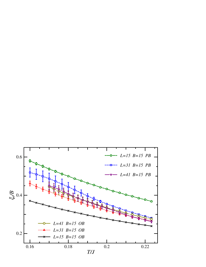
Figure 1: (Color online) Results of window measurements in static simulations. The SG correlation-length ratio, $\xi_{\rm s}/B$, is plotted against the temperature. $B$ is a size of window. PB and OB stand for periodic boundary and open boundary conditions.

Results- First, we show the static simulation data. The equilibrium SG correlation-length ratio, $\xi_{\mathrm{s}}/B$, is plotted against the temperature when $B=15$ in Fig. 1. The equilibrium values depend on the boundary conditions when $B=L$. As $L$ increases, the window-measurement data of PB and OB approach each other. The data of $L=41$ are independent of the boundary conditions. We obtain similar results for the equilibrium CG correlation length ratio and the distribution function of order parameters. We can neglect the boundary effects if we set $B/L<1/3$. So, what we have to do is the following procedures: (i) set the window ratio as $B/L=1/3$; (ii) collect equilibrium data for different $B$; (iii) perform the finite-$B$ scaling analyses. However, this procedure does not sound realistic because the equilibrium simulation up to now is restricted to $L=48$, which gives the upper bound for $B$ is 16. Therefore, we adopt a dynamic scaling approachNerReview ; ozekiito-SG ; nakamura5 ; yamamoto1 ; nakamura4 that can handle larger lattice sizes. We also try to relax the ratio requirement, $B/L<1/3$, which discards most of the simulated spins.

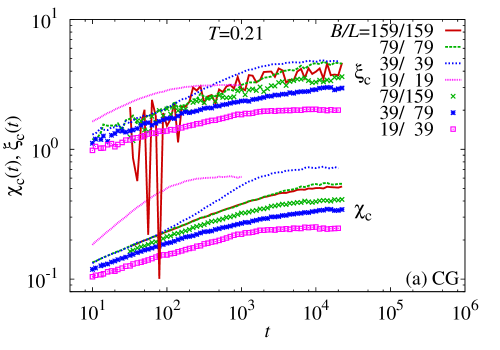
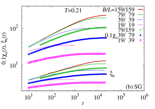
Figure 2: (Color online) Relaxation functions of the susceptibility and the correlation length for whole measurements (lines) and window measurements (symbols). Error bars are smaller than line width for SG data but they are in a same order as data fluctuation for CG data.

Figure  2 shows a dynamic simulation result. We plot relaxation functions of (a) $\chi_{\rm c}$ and $\xi_{\rm c}$, and (b) $\chi_{\rm s}$ and $\xi_{\rm s}$. The temperature, $T=0.21$, is considered as in a paramagnetic phase but close to the transition temperature.nakamura ; HukushimaH2 As was observed in the Ising SG model,hukushimacampbell we find a size-crossover effect in relaxation data of $\chi_{\mathrm{c}}(t)$ when $B=L$, while there is no size crossover when $B<L$. A converging value takes a maximum when $B=L=39$ and it decreases as $L$ increases or decreases. They also deviate to the upper side when the finite-size effects appear. It suggests that the finite-size scaling analyses using data of $L$ smaller than 39 should be carefully performed. It is also noted that an amplitude of each relaxation function depends on $B$, $L$, and $B/L$. If we fix $B$ and compare the window-measurement results and the whole-measurement results (lines and symbols with same color in Fig. 2), we find that the window results always take smaller values than the whole results. Both results for $\chi_{\rm c}$ approach each other as $B$ increases but those for $\chi_{\rm s}$ do not. These dependences are quantitatively complicated. This ambiguity may be a reason why the window measurement scheme has not been applied to the scaling analyses.

We apply the dynamic-correlation-length scaling analysisnakamuraxisca to the window measurements. A relaxation function of the susceptibility is plotted against that of the correlation length. It should show an algebraic divergence as $\chi\sim\xi^{2-\eta}$ at the second-order transition temperature. It is a straight line if we plot it in a log-log scale. It exhibits a downward-bending behavior in the paramagnetic phase and an upward-bending behavior in the ordered phase.

Figure 3 shows finite-time and finite-size relaxation data of $\chi_{\rm s/c}(t,L)$ plotted against $\xi_{\rm s/c}(t,L)$. We also plot equilibrium data with OB conditions. Here, the CG results of $L=159$ are omitted because the $\xi_{\rm c}$ data include large numerical fluctuation as shown in Fig. 2(a). In this figure we find that all the SG window-measurement data (nonequilibrium data of $B/L=4/5$–$1/3$ for $L=19$–$159$ and equilibrium data of $B=10$ and 15 for $L=31$ and 41) ride on a single scaling function. Equilibrium data of small sizes appear on the way of nonequilibrium relaxation data of large sizes. It can be considered that the SG susceptibility increases in accordance with the SG correlation length in a uniform manner. Size and time, which are man-made parameters, do not matter much. This scaling function is expected to continue smoothly to the thermodynamic limit. In other words, the correction-to-scaling terms are considered as very small. This is an advantage of the window measurement and the correlation-length scaling. As a result, the $B/L$ ratios can be set larger than $1/3$ up to $4/5$. This improves the computational efficiency. To the contrary, the whole-measurement data ($B/L=1/1$; $L=19$–$159$) show size dependences. Small-size data deviate to the upper side and only the largest-size data exhibit the downward bending. We may need still larger lattices in the whole-measurement scheme to observe size-independent thermodynamic behaviors.

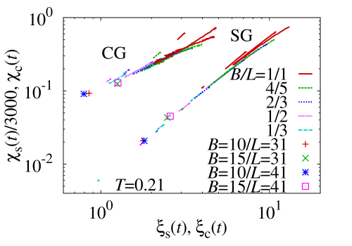
Figure 3: (Color online) Relaxation functions of the susceptibility are plotted against those of the correlation length. Each line type corresponds to each $B/L$ ratio for all the systems sizes, $L=$19, 39, 79 and 159(SG only). Static simulation data of $B=10$ and 15 for $L=31$ and 41 with OB conditions are also plotted with symbols. Error bars are smaller than line width and symbols.

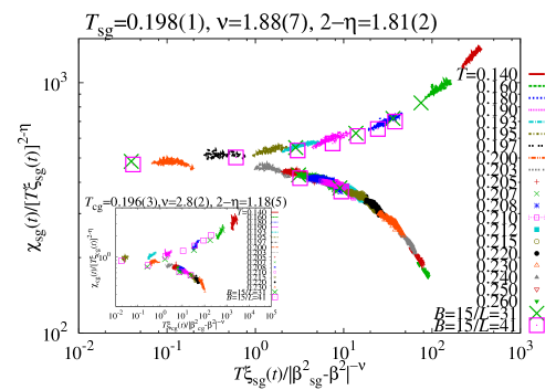
Figure 4: (Color online) A dynamic scaling plot of the SG susceptibility and SG correlation lengths. Nonequilibrium data of $B/L=4/5,2/3,1/2$, $1/3$ with $L=79$ and 159, and equilibrium data of $B=15$ with $L=31$ and 41(OB conditions) are plotted for each temperature. The first 200 steps are discarded for nonequilibrium data. An inset is the scaling plot for CG (up to $L=79$). Error bars are smaller than line width and symbols.

Since the correction-to-scaling terms are considered to be small in the window measurements, we can use all the finite-size and the finite-time relaxation data of $\chi$ and $\xi$ for the dynamic scaling analysis to determine the transition temperature and critical exponents. Figure 4 is the scaling plot. The scaling parameters are estimated by the Bayesian inference introduced by Haradaharada . We randomly choose 600 datasets of $(\chi(t),\xi(t))$ out of 2798 entries for $L=79$ and 159 for SG, and performed the inference for 40 times changing the datasets and initial values of estimated parameters. The $\beta$-scaling method proposed by Campbell et al.campbell-huku-taka is also applied. The estimated SG transition temperature is located between the one obtained by Matsubara et al.matsubara3 ($T_{\rm sg}=0.18$) and the one obtained by Nakamura and Endohnakamura ($T_{\rm sg}=0.21$). We plot equilibrium data of $B=15$ for $L=31$ and 41 using the scaling parameters estimated by the nonequilibrium data. They ride on the same scaling function very well. It is noted that data of $B=10$ systematically deviate to the lower side. We consider that there exists a lower bound size that can be used in the scaling analysis. It may be located between 10 and 15. The scaling plot of CG is similar to that of SG. We performed the scaling inference using only the $L=79$ data. An estimate of $T_{\rm cg}$ is very close to $T_{\rm sg}$. It is also consistent with the one obtained by Hukushima and KawamuraHukushimaH2 , which gave $T_{\rm cg}=0.194$. Therefore, the present results suggest the simultaneous spin-chirality transition.

Summary and Discussion- We have proposed a window measurement scheme, which practically solves severe finite-size and finite-time effects. The correction-to-scaling terms sometimes cause discrepancies in the final result of scaling analyses. They can be made very small by scaling the window data with the window correlation length. We can also combine equilibrium data of small sizes and nonequilibrium data of large sizes into one scaling analysis. It is a great advantage in the slow-dynamic systems.

In exchange for the benefit of the window measurements, we must accept a big waste of computations. Almost a half of total spins are discarded even when $B/L=0.8$ in three dimensions. If $B/L=1/3$, this discard ratio becomes 96%! However, a recent progress in high-performance computers drastically dropped the computational cost and allowed us to accept the waste. We performed the present simulations by CUDA GPGPU environment developed by Nvidia. We could easily achieve 10 times faster simulations by a GPU with a reasonable price (additional $499 per node). A rich man’s algorithm that can accept the waste may be a standard approach in computational physics from now on.

The window measurement scheme can be applied to incommensurate systems and long-range interacting systems, where finite-size effects are also severe. It may be promising to apply it to the two-dimensional frustrated quantum spin systems, where the treated sizes are also limited.kagome As for the Heisenberg SG problem, we observed a simultaneous spin-chirality transition. We also found a size crossoverhukushimacampbell in the CG susceptibility.

- (1) D. P. Landau and K. Binder, A Guide to Monte Carlo Simulations in Statistical Physics (Cambridge University Press, Cambridge, 2005), 2nd ed.
- (2) Y. Komura and Y. Okabe, J. Phys. Soc. Jpn. 81, 113001 (2012).
- (3) Spin Glasses and Random Fields, ed. A. P. Young (World Scientific, Singapore, 1997).
- (4) N. Kawashima and H. Rieger, in Frustrated Spin Systems, ed. H. T. Diep (World Scientific, Sigapore, 2004).
- (5) K. Hukushima and K. Nemoto, J. Phys. Soc. Jpn. 65, 1604 (1996).
- (6) L. A. Fernandez, V. Martin-Mayor, S. Perez-Gaviro, A. Tarancon, and A. P. Young, Phys. Rev. B 80, 024422 (2009).
- (7) D. X. Viet and H. Kawamura, Phys. Rev. Lett. 102, 027202 (2009).
- (8) D. X. Viet and H. Kawamura, Phys. Rev. B 80, 064418 (2009).
- (9) J. A. Olive, A. P. Young, and D. Sherrington, Phys. Rev. B 34, 6341 (1986).
- (10) H. Kawamura, Phys. Rev. Lett. 68, 3785 (1992).
- (11) K. Hukushima and H. Kawamura, Phys. Rev. E 61, R1008 (2000).
- (12) F. Matsubara, S. Endoh, and T. Shirakura, J. Phys. Soc. Jpn. 69, 1927 (2000).
- (13) S. Endoh, F. Matsubara, and T. Shirakura, J. Phys. Soc. Jpn. 70, 1543 (2001).
- (14) F. Matsubara, T. Shirakura, and S. Endoh, Phys. Rev. B 64, 092412 (2001).
- (15) M. Matsumoto, K. Hukushima, and H. Takayama, Phys. Rev. B 66, 104404 (2002).
- (16) T. Nakamura and S. Endoh, J. Phys. Soc. Jpn. 71, 2113 (2002).
- (17) L. W. Lee and A. P. Young, Phys. Rev. Lett. 90, 227203 (2003).
- (18) L. Berthier and A. P. Young, Phys. Rev. B 69, 184423 (2004).
- (19) M. Picco and F. Ritort, Phys. Rev. B 71, 100406(R) (2005).
- (20) K. Hukushima and H. Kawamura, Phys. Rev. B 72, 144416 (2005).
- (21) I. Campos, M. Cotallo-Aban, V. Martin-Mayor, S. Perez-Gaviro, and A. Tarancon, Phys. Rev. Lett. 97, 217204 (2006).
- (22) L. W. Lee and A. P. Young, Phys. Rev. B 76, 024405 (2007).
- (23) R. N. Bhatt and A. P. Young, Phys. Rev. Lett. 54, 924 (1985).
- (24) A. T. Ogielski and I. Morgenstern, Phys. Rev. Lett. 54, 928 (1985).
- (25) N. Kawashima and A. P. Young, Phys. Rev. B 53, R484 (1996).
- (26) M. Palassini and S. Caracciolo, Phys. Rev. Lett. 82 5128 (1999).
- (27) H. G. Ballesteros, A. Cruz, L. A. Fernández, V. Martin-Mayor, J. Pech, J. J. Ruiz-Lorenzo, A. Tarancón, P. Téllez, C. L. Ullod, and C. Ungil, Phys. Rev. B 62, 14 237 (2000).
- (28) P. O. Mari and I. A. Campbell, Phys. Rev. B 65, 184409 (2002).
- (29) T. Nakamura, S. Endoh, and T. Yamamoto, J. Phys. A 36, 10 895 (2003).
- (30) I. A. Campbell, K. Hukushima, and H. Takayama, Phys. Rev. Lett. 97, 117202 (2006).
- (31) M. Hasenbusch, A. Pelissetto, and E. Vicari, Phys. Rev. B 78, 214205 (2008).
- (32) T. Nakamura, Phys. Rev. B 82, 014427 (2010).
- (33) K. Hukushima and I. A. Campbell, arXiv:0903.5026v1.
- (34) T. Shirakura and F. Matsubara, J. Phys. Soc. Jpn. 79, 075001 (2010).
- (35) C. M. Newman and D. L. Stein, Phys. Rev. E 57, 1356 (1998).
- (36) E. Marinari, G. Parisi, F. Ricci-Tersenghi, and J. J. Ruiz-Lorenzo, J. Phys. A: Math. Gen. 31, L481 (1998).
- (37) L. S. Ornstein and F. Zernike, Proc. R. Acad. Sci. Amsterdam 17, 793 (1914).
- (38) Y. Ozeki and N. Ito, J. Phys. A 40, R149 (2007).
- (39) Y. Ozeki and N. Ito, Phys. Rev. B 64, 024416 (2001).
- (40) T. Nakamura, J. Phys. Soc. Jpn. 72, 789 (2003).
- (41) T. Yamamoto, T. Sugashima, and T. Nakamura, Phys. Rev. B 70, 184417 (2004).
- (42) T. Nakamura, Phys. Rev. B 71, 144401 (2005).
- (43) K. Harada, Phys. Rev. E 84, 056704 (2011).
- (44) H. Nakano and T. Sakai, J. Phys. Soc. Jpn. 80, 053704 (2011).