Continuous Matrix Approximation on Distributed Data

Tracking and approximating data matrices in streaming fashion is a fundamental challenge. The problem requires more care and attention when data comes from multiple distributed sites, each receiving a stream of data. This paper considers the problem of “tracking approximations to a matrix” in the distributed streaming model. In this model, there are $m$ distributed sites each observing a distinct stream of data (where each element is a row of a distributed matrix) and has a communication channel with a coordinator, and the goal is to track an $\varepsilon$-approximation to the norm of the matrix along any direction. To that end, we present novel algorithms to address the matrix approximation problem. Our algorithms maintain a smaller matrix $B$, as an approximation to a distributed streaming matrix $A$, such that for any unit vector $x$: $|\|Ax\|^{2}-\|Bx\|^{2}|\leq\varepsilon\|A\|_{F}^{2}$. Our algorithms work in streaming fashion and incur small communication, which is critical for distributed computation. Our best method is deterministic and uses only $O((m/\varepsilon)\log(\beta N))$ communication, where $N$ is the size of stream (at the time of the query) and $\beta$ is an upper-bound on the squared norm of any row of the matrix. In addition to proving all algorithmic properties theoretically, extensive experiments with real large datasets demonstrate the efficiency of these protocols.

1 Introduction

Large data matrices are found in numerous domains, such as scientific computing, multimedia applications, networking systems, server and user logs, and many others [28, 36, 26, 27]. Since such data is huge in size and often generated continuously, it is important to process them in streaming fashion and maintain an approximating summary. Due to its importance, the matrix approximation problem has received careful investigations in the literature; the latest significant effort is represented by Liberty [28] on a centralized stream.

In recent years, distributed streaming model [14] has become popular, in which there are multiple distributed sites, each observing a disjoint stream of data and together attempt to monitor a function at a single coordinator site $C$. Due to its wide applications in practice [14], a flurry of work has been done under this setting. This model is more general than the streaming model [3] that maintains a function at a single site with small space. It is also different from communication model [42] in which data is (already) stored at multiple sites and the goal is to do a one-time computation of a target function. The key resources to optimize in distributed streaming model is not just the space needed at the coordinator or each site, but the communication between the sites and coordinator.

Despite prior works on distributed streaming model, and distributed matrix computations (e.g., the MadLINQ library [38]), little is known on continuously tracking an matrix approximation in the distributed streaming model. This paper considers the important problem of “tracking approximations to matrices” in the distributed streaming model [14].

Motivation.

Our problem is motivated by many applications in distributed databases, wireless sensor networks, cloud computing, etc [34] where data sources are distributed over a network and collecting all data together at a central location is not a viable option. In many such environments queries must be answered continuously, based on the total data that has arrived so far.

For example, in large scale image analysis, each row in the matrix corresponds to one image and contains either pixel values or other derived feature values (e.g, 128-dimensional SIFT features). A search engine company has image data continuously arriving at many data centers, or even within a single data center at many nodes in a massive cluster. This forms a distributed matrix and it is critical to obtain excellent, real-time approximation of the distributed streaming image matrix with little communication overhead.

Yet another example is for large-scale distributed web crawling or server access log monitoring/mining, where data in the bag-of-words model is a matrix whose columns correspond to words or tags/labels (for textual analysis, e.g. LSI, and/or for learning and classification purpose) and rows correspond to documents or log records (which arrive continuously at distributed nodes).

Since data is continuously changing in these applications, query results can also change with time. So the challenge is to minimize the communication between sites and the coordinator while maintaining accuracy of results at all time.

In our case, each site may generate a record in a given time instance, which is a row of a matrix. The goal is to approximate the matrix that is the union of all the rows from all sites until current time instance $t_{\textrm{now}}$ continuously at the coordinator $C$. This problem can be easily found in distributed network monitoring applications [37], distributed data mining, cloud computing [38], stream mining [23], and log analysis from multiple data centers [9].

Distributed streaming matrix approximation.

Formally, assume $A=(a_{1},\ldots,a_{n},\ldots)$ is an unbounded stream of items. At the current time $t_{\textrm{now}}$, let $n$ denote the number of items the system has seen so far; that is at the current time the dataset is $A=(a_{1},\ldots,a_{n})$. And although we do not place a bound on the number of items, we let $N$ denote the total size of the stream at the time when a query $q$ is performed. This allows us to discuss results in terms of $n$ at a given point, and in terms of $N$ for the entire run of the algorithm until the time of a query $q$.

At each time step we assume the item $a_{n}$ appears at exactly one of $m$ sites $S_{1},\ldots,S_{m}$. The goal is to approximately maintain or monitor some function $f(A)$ of $A$ at the coordinator node $C$. Each site can only communicate with the coordinator (which in practice may actually be one of the sites). This model is only off by a factor $2$ in communication with a model where all pairs of sites can communicate, by routing through the coordinator.

Our goal is to maintain a value $\hat{f}(A)$ which is off by some $\varepsilon$-factor from the true value $f(A)$. The function and manner of approximation is specified for a variety of problems [43, 30, 25, 4, 12, 11] included total count, heavy hitters, quantiles, and introduced in this paper, matrix approximation:

Definition 1 (Tracking distributed streaming matrix)

:
Suppose each $a_{n}$ is a record with $d$ attributes, a row from a matrix in an application. Thus, at time $t_{\textrm{now}}$, $A=(a_{1},\ldots,a_{n})$ forms a $n\times d$ distributed streaming matrix. At any time instance, $C$ needs to approximately maintain the norm of matrix $A$ along any arbitrary direction. The goal is to continuously track a small approximation of matrix $A$. Formally, for any time instance $t_{\textrm{now}}$ (i.e., for any $n$), $C$ needs to maintain a smaller matrix $B\in\mathbb{R}^{\ell\times d}$ as an approximation to the distributed streaming matrix $A\in\mathbb{R}^{n\times d}$ such that $\ell\ll n$ and for any unit vector $x$: $|\|Ax\|^{2}-\|Bx\|^{2}|\leq\varepsilon\|A\|_{F}^{2}$.

As required in the distributed streaming model [14], each site $S_{i}$ must process its incoming elements in streaming fashion. The objective is to minimize the total communication between $C$ and all sites $S_{1},\ldots,S_{m}$. ∎

Additional notations.

In the above definition, the Frobenius norm of a matrix $A$ is $\|A\|_{F}=\sqrt{\sum_{i=1}^{n}\|a_{i}\|^{2}}$ where $\|a_{i}\|$ is standard Euclidean norm of row $a_{i}$; the Frobenius norm is a widely used matrix norm. We also let $A_{k}$ be the best rank $k$ approximation of matrix $A$, specifically $A_{k}={\arg\min}_{X:{\textsf{rank}}(X)\leq k}\|A-X\|_{F}$.

Our contributions.

This work makes important contributions in solving the open problem of tracking distributed streaming matrix. Instead of exploring heuristic methods that offer no guarantees on approximation quality, we focus on principled approaches that are built on sound theoretical foundations. Moreover, all methods are simple and efficient to implement as well as effective in practice. Specifically:

• We establish and further the important connection between tracking a matrix approximation and maintaining $\varepsilon$-approximate weighted heavy-hitters in the distributed streaming model in Section 4. Initial insights along this direction were established in very recent work [28, 21]; but the extent of this connection is still limited and not fully understood. This is demonstrated, for instance, by us showing how three approaches for weighted heavy hitters can be adapted to matrix sketching, but a fourth cannot.

• We introduce four new methods for tracking the $\varepsilon$-approximate weighted heavy-hitters in a distributed stream in Section 4, and analyze their behaviors with rigorous theoretical analysis.

• We design three novel algorithms for tracking a good approximation of a distributed streaming matrix in Section 5; these leverage the new insights connecting this problem to solutions in Section 4 for distributed weighted heavy hitters tracking.

• We present thorough experimental evaluations of the proposed methods in Section 6 on a number of large real data sets. Experimental results verify the effectiveness of our methods in practice.

In addition, we provide a thorough review of related works and relevant background material in Section 2. The paper is concluded in Section 7.

2 Related work

There are two main classes of prior work that are relevant to our study: approximating a streaming matrix in a centralized stream, and tracking heavy hitters in either a centralized stream or (the union of) distributed steams.

Matrix approximation in a centralized stream.

Every incoming item in a centralized stream represents a new row of data in a streaming matrix. The goal is to continuously maintain a low rank matrix approximation. It is a special instance of our problem for $m=1$, i.e., there is only a single site. Several results exist in the literature, including streaming PCA (principal component analysis) [33], streaming SVD (singular value decomposition) [39, 7], and matrix sketching [8, 28, 21]. The matrix sketching technique [28] only recently appeared and is the start-of-the-art for low-rank matrix approximation in a single stream. Liberty [28] adapts a well-known streaming algorithm for approximating item frequencies, the MG algorithm [32], to sketching a streaming matrix. The method, Frequent Directions (FD), receives $n$ rows of a matrix $A\in\mathbb{R}^{n\times d}$ one after another, in a centralized streaming fashion. It maintains a sketch $B\in\mathbb{R}^{\ell\times d}$ with only $\ell\ll n$ rows, but guarantees that $A^{T}A\approx B^{T}B$. More precisely, it guarantees that $\forall x\in\mathbb{R}^{d}$, $\|x\|=1$, $0\leq\|Ax\|^{2}-\|Bx\|^{2}\leq 2\|A\|^{2}_{F}/\ell$. FD uses $O(d\ell)$ space, and each item updates the sketch in amortized $O(d\ell)$ time; two such sketches can also be merged in $O(d\ell^{2})$ time.

A bound on $\|Ax\|$ for any unit vector $x$ preserves norm (or length) of a matrix in direction $x$. For instance, when one performs PCA on $A$, it returns the set of the top $k$ orthogonal directions, measured in this length. These are the linear combinations of attributes (here we have $d$ such attributes) which best capture the variation within the data in $A$. Thus by increasing $\ell$, this bound allows one to approximately retain all important linear combinations of attributes.

An extension of FD to derive streaming sketch results with bounds on relative errors, i.e., to ensure that $\|A-A_{k}\|_{F}^{2}\leq\|A\|_{F}^{2}-\|B_{k}\|_{F}^{2}\leq(1+\varepsilon)\|A-A_{k}\|_{F}^{2}$, appeared in [21]. It also gives that $\|A-\pi_{B_{k}}(A)\|_{F}^{2}\leq(1+\varepsilon)\|A-A_{k}\|^{2}_{F}$ where $B_{k}$ is the top $k$ rows of $B$ and $\pi_{B_{k}}(A)$ is the projection of $A$ onto the row-space of $B_{k}$. This latter bound is interesting because, as we will see, it indicates that when most of the variation is captured in the first $k$ principal components, then we can almost recover the entire matrix exactly.

But none of these results can be applied in distributed streaming model without incurring high communication cost. Even though the FD sketches are mergeable, since the coordinator $C$ needs to maintain an approximation matrix continuously for all time instances. One has to either send $m$ sketches to $C$, one from each site, at every time instance and ask $C$ to merge them to a single sketch, or one can send a streaming element to $C$ whenever it is received at a site and ask $C$ to maintain a single sketch using FD at $C$. Either approach will lead to $\Omega(N)$ communication.

Nevertheless, the design of FD has inspired us to explore the connection between distributed matrix approximation and approximation of distributed heavy hitters.

Heavy hitters in distributed streams.

Tracking heavy hitters in distributed streaming model is a fundamental problem [43, 30, 25, 4]. Here we assume each $a_{n}\in A$ is an element of a bounded universe $[u]=\{1,\ldots,u\}$. If we denote the frequency of an element $e\in[u]$ in the stream $A$ as $f_{e}(A)$, the $\phi$-heavy hitters of $A$ (at time instance $t_{\textrm{now}}$) would be those items $e$ with $f_{e}(A)\geq\phi n$ for some parameter $\phi\in[0,1]$. We denote this set as $H_{\phi}(A)$. Since computing exact $\phi$-heavy hitters incurs high cost and is often unnecessary, we allow an $\varepsilon$-approximation, then the returned set of heavy hitters must include $H_{\phi}(A)$, may or may not include items $e$ such that $(\phi-\varepsilon)n\leq f_{e}(A)<\phi n$ and must not include items $e$ with $f_{e}(A)<(\phi-\varepsilon)n$.

Babcock and Olston [4] designed some deterministic heuristics called as top-$k$ monitoring to compute top-$k$ frequent items. Fuller and Kantardzid modified their technique and proposed FIDS [20], a heuristic method, to track the heavy hitters while reducing communication cost and improving overall quality of results. Manjhi et al.[30] studied $\phi$-heavy hitter tracking in a hierarchical communication model.

Cormode and Garofalakis [11] proposed another method by maintaining a summary of the input stream and a prediction sketch at each site. If the summary varies from the prediction sketch by more than a user defined tolerance amount, the summary and (possibly) a new prediction sketch is sent to a coordinator. The coordinator can use the information gathered from each site to continuously report frequent items. Sketches maintained by each site in this method require $O((1/\varepsilon^{2})\log(1/\delta))$ space and $O(\log(1/\delta))$ time per update, where $\delta$ is a probabilistic confidence.

Yi and Zhang [43] provided a deterministic algorithm with communication cost $O((m/\varepsilon)\log N)$ and $O(1/\varepsilon)$ space at each site to continuously track $\phi$-heavy hitters and the $\phi$-quantiles. In their method, every site and the coordinator have as many counters as the type of items plus one more counter for the total items. Every site keeps track of number of items it receives in each round, once this number reaches roughly $\varepsilon/m$ times of the total counter at the coordinator, the site sends the counter to the coordinator. After the coordinator receives $m$ such messages, it updates its counters and broadcasts them to all sites. Sites reset their counter values and continue to next round. To lower space usage at sites, they suggested using space-saving sketch[31]. The authors also gave matching lower bounds on the communication costs for both problems, showing their algorithms are optimal in the deterministic setting.

Later, Huang et al. [22] proposed a randomized algorithm that uses $O(1/(\varepsilon\sqrt{m}))$ space at each site and $O((\sqrt{m}/\varepsilon)\log N)$ total communication and tracks heavy hitters in a distributed stream. For each item $a$ in the stream a site chooses to send a message with a probability $p=\sqrt{m}/(\varepsilon\hat{n})$ where $\hat{n}$ is a $2$-approximation of the total count. It then sends $f_{e}(A_{j})$ the total count of messages at site $j$ where $a=e$, to the coordinator. Again an approximation heavy-hitter count $\hat{f}_{e}(A_{j})$ can be used at each site to reduce space.

The $\varepsilon$-heavy hitters can be maintained from a random sampling of elements of size $s=O(1/\varepsilon^{2})$. This allows one to use the well studied technique of maintaining a random sample of size $s$ from a distributed stream [15, 41], which can be done with roughly $O((m+s)\log(N/s))$ communication.

Other related work.

Lastly, our work falls into the general problem of tracking a function in distributed streaming model. Many existing works have studied this general problem for various specific functions, and we have reviewed the most related ones on heavy hitters. A detailed survey of results on other functions (that are much less relevant to our study) is beyond the scope of this work, and we refer interested readers to [14, 10] and references therein.

Our study is also related to various matrix computations over distributed matrices, for example, the MadLINQ library [38]. However, these results focus on one-time computation over non-streaming data, i.e., in the communication model [42] as reviewed in Section 1. We refer interested readers to [38] and references therein for details.

There are also many studies on low-rank approximations of matrices in centralized, non-streaming setting, e.g., [29, 19, 1, 16] and others, but these methods are not applicable for a distributed streaming setting.

3 Insights, Weights and Rounds

A key contribution of this paper is strengthening the connection between maintaining approximate weighted frequency counts and approximately maintaining matrices.

To review, the Misra-Gries (MG) algorithm [32] is a deterministic, associative sketch to approximate frequency counts, in contrast to, say the popular count-min sketch [13] which is randomized and hash-based. MG maintains an associative array of size $\ell$ whose keys are elements of $e\in[u]$, and values are estimated frequency $\hat{f}_{e}$ such that $0\leq f_{e}-\hat{f}_{e}\leq n/\ell$. Upon processing element $e\in A$, three cases can occur. If $e$ matches a label, it increments the associated counter. If not, and there is an empty counter, it sets the label of the counter to $e$ and sets its counter to $1$. Otherwise, if no empty counters, then it decrements (shrinks) all counters by $1$.

Liberty [28] made this connection between frequency estimates and matrices in a centralized stream through the singular value decomposition (svd). Our approaches avoid the svd or use it in a different way. The svd of an $n\times d$ matrix $A$ returns (among other things) a set of $d$ singular values $\{\sigma_{1}\geq\sigma_{2}\geq\ldots\geq\sigma_{d}\}$ and a corresponding set of orthogonal right singular vectors $\{v_{1},\ldots,v_{d}\}$. It holds that $\|A\|_{F}^{2}=\sum_{i=1}^{d}\sigma_{i}^{2}$ and for any $x$ that $\|Ax\|^{2}=\sum_{i=1}^{d}\sigma_{i}^{2}\langle v_{i},x\rangle^{2}$. The work of Liberty [28] shows that one can run a version of the Misra-Gries [32] sketch for frequency counts using the singular vectors as elements and squared singular values as the corresponding total weights, recomputing the svd when performing the shrinkage step.

To see why this works, let us consider the restricted case where every row of the matrix $A$ is an indicator vector along the standard orthonormal basis. That is, each row $a_{i}\in\{e_{1},\ldots,e_{d}\}$, where $e_{j}=(0,\ldots,0,1,0,\ldots,0)$ is the $j$th standard basis vector. Such a matrix $A$ can encode a stream $S$ of items from a domain $[d]$. If the $i$th element in the stream $S$ is item $j\in\{1,\ldots,d\}$, then the $i$th row of the matrix $A$ is set to $a_{i}=e_{j}$. At time $t_{\textrm{now}}$, the frequency $f_{j}$ from $S$ can be expressed as $f_{j}=\|Ae_{j}\|^{2}$, since $\|Ax\|^{2}=\sum_{i=1}^{n}\langle a_{i},x\rangle^{2}$ and the dot product is only non-zero in this matrix for rows which are along $e_{j}$. A good approximate matrix $B$ would be one such that $g_{j}=\|Be_{j}\|^{2}$ is a good approximation of $f_{j}$. Given $\|A\|_{F}^{2}=n$ (since each row of $A$ is a standard basis vector), we derive that $|f_{j}-g_{j}|\leq\varepsilon n$ is equivalent to $|\|Ae_{j}\|^{2}-\|Be_{j}\|^{2}|\leq\varepsilon\|A\|_{F}^{2}$.

However, general matrices deviate from this simplified example in having non-orthonormal rows. Liberty’s FD algorithm [28] demonstrates how taking svd of a general matrix gets around this deviation and it achieves the same bound $|\|Ax\|^{2}-\|Bx\|^{2}|\leq\varepsilon\|A\|_{F}^{2}$ for any unit vector $x$.

Given the above connection, in this paper, first we propose four novel methods for tracking weighted heavy hitters in a distributed stream of items (note that tracking weighted heavy hitters in the distributed streaming model has not been studied before). Then, we try to extend them to track matrix approximations where elements of the stream are $d$-dimensional vectors. Three extensions are successful, including one based directly on Liberty’s algorithm, and two others establishing new connections between weighted frequency estimation and matrix approximation. We also show why the fourth approach cannot be extended, illustrating that the newly established connections are not obvious.

Upper bound on weights.

As mentioned above, there are two main challenges in extending ideas from frequent items estimation to matrix approximation. While, the second requires delving into matrix decomposition properties, the first one is in dealing with weighted elements. We discuss here some high-level issues and assumptions we make towards this goal.

In the weighted heavy hitters problem (similarly in matrix approximation problem) each item $a_{i}$ in the stream has a weight $w_{i}$ (for matrices this weight will be implicit as $\|a_{i}\|^{2}$). Let $W=\sum_{i=1}^{n}w_{i}$ be the total weight of the problem. However, allowing arbitrary weights can cause problems as demonstrated in the following example.

Suppose we want to maintain a $2$-approximation of the total weight (i.e. a value $\hat{W}$ such that $\hat{W}\leq W\leq 2\hat{W}$). If the weight of each item doubles (i.e. $w_{i}=2^{i}$ for tuple $(a_{i},w_{i})\in A$), every weight needs to be sent to the coordinator. This follows since $W$ more than doubles with every item, so $\hat{W}$ cannot be valid for more than one step. The same issue arises in tracking approximate heavy hitters and matrices.

To make these problems well-posed, often researchers [24] assume weights vary in a finite range, and are then able to bound communication cost. To this end we assume all $w_{i}\in[1,\beta]$ for some constant $\beta\geq 1$.

One option for dealing with weights is to just pretend every item with element $e$ and weight $w_{i}$ is actually a set of $\lceil w_{i}\rceil$ distinct items of element $e$ and weight $1$ (the last one needs to be handled carefully if $w_{i}$ is not an integer). But this can increase the total communication and/or runtime of the algorithm by a factor $\beta$, and is not desirable.

Our methods take great care to only increase the communication by a $\log(\beta N)/\log N$ factor compared to similar unweighted variants. In unweighted version, each protocol proceeds in $O(\log N)$ rounds (sometimes $O(\frac{1}{\varepsilon}\log N)$ rounds); a new round starts roughly when the total count $n$ doubles. In our settings, the rounds will be based on the total weight $W$, and will change roughly when the total weight $W$ doubles. Since the final weight $W\leq\beta N$, this will causes an increase to $O(\log W)=O(\log(\beta N))$ rounds. The actual analysis requires much more subtlety and care than described here, as we will show in this paper. Next we first discuss the weighted heavy-hitters problem, as the matrix tracking problem will directly build on these techniques, and some analysis will also carry over directly.

4 Weighted Heavy Hitters in A Distributed Stream

The input is a distributed weighted data stream $A$, which is a sequence of tuples $(a_{1},w_{1}),(a_{2},w_{2}),\ldots,(a_{n},w_{n}),\ldots$ where $a_{n}$ is an element label and $w_{n}$ is the weight. For any element $e\in[u]$, define $A_{e}=\{(a_{i},w_{i})\mid a_{i}=e\}$ and let $W_{e}=\sum_{(a_{i},w_{i})\in A_{e}}w_{i}$. For notational convenience, we sometimes refer to a tuple $(a_{i},w_{i})\in A$ by just its element $a_{i}$.

There are numerous important motivating scenarios for this extension. For example, instead of just monitoring counts of objects, we can measure a total size associated with an object, such as total number of bytes sent to an IP address, as opposed to just a count of packets. We next describe how to extend four protocols for heavy hitters to the weighted setting. These are extensions of the unweighted protocols described in Section 2.

Estimating total weight.

An important task is to approximate the current total weight $W=\sum_{i=1}^{n}w_{i}$ for all items across all sites. This is a special case of the heavy hitters problem where all items are treated as being the same element. So if we can show a result to estimate the weight of any single element using a protocol within $\varepsilon W$, then we can get a global estimate $\hat{W}$ such that $|W-\hat{W}|\leq\varepsilon W$. All our subsequent protocols can run a separate process in parallel to return this estimate if they do not do so already.

Recall that the heavy hitter problem typically calls to return all elements $e\in[u]$ if $f_{e}(A)/W\geq\phi$, and never if $f_{e}(A)/W<\phi-\varepsilon$. For each protocol we study, the main goal is to ensure that an estimate $\hat{W}_{e}$ satisfies $|f_{e}(A)-\hat{W}_{e}|\leq\varepsilon W$. We show this, along with the $\hat{W}$ bound above, adjusting constants, is sufficient to estimate weighted heavy hitters. We return $e$ as a $\phi$-weighted heavy hitter if $\hat{W}_{e}/\hat{W}>\phi-\varepsilon/2$.

Lemma 1

If $|f_{e}(A)-\hat{W}_{e}|\leq(\varepsilon/6)W$ and $|W-\hat{W}|\leq(\varepsilon/5)W$, we return $e$ if and only if it is a valid weighted heavy hitter.

Proof.

We need $|\frac{\hat{W}_{e}}{\hat{W}}-\frac{f_{e}(A)}{W}|\leq\varepsilon/2$. We show the upper bound, the lower bound argument is symmetric.

$$\frac{\hat{W}_{e}}{\hat{W}} \leq\frac{f_{e}(A)}{\hat{W}}+\frac{\varepsilon}{6}\frac{W}{\hat{W}}\leq\frac{f_{e}(A)}{W}\frac{1}{1-\varepsilon/5}+\frac{\varepsilon}{5}\frac{1+\varepsilon/5}{1-\varepsilon/5}$$

$$\leq\frac{f_{e}(A)}{W}+\frac{\varepsilon}{4}+\frac{\varepsilon}{4}=\frac{f_{e}(A)}{W}+\frac{\varepsilon}{2}.\qed$$

∎

Given this result, we can focus just on approximating the frequency $f_{e}(A)$ of all items.

4.1 Weighted Heavy Hitters, Protocol 1

We start with an intuitive approach to the distributed streaming problem: run a streaming algorithm (for frequency estimation) on each site, and occasionally send the full summary on each site to the coordinator. We next formalize this protocol (P1).

On each site we run the Misha-Gries summary [32] for frequency estimation, modified to handle weights, with $2/\varepsilon=1/\varepsilon^{\prime}$ counters. We also keep track of the total weight $W_{i}$ of all data seen on that site $i$ since the last communication with the coordinator. When $W_{i}$ reaches a threshold $\tau$, site $i$ sends all of its summaries (of size only $O(m/\varepsilon)$) to the coordinator. We set $\tau=(\varepsilon/2m)\hat{W}$, where $\hat{W}$ is an estimate of the total weight across all sites, provided by the coordinator. At this point the site resets its content to empty. This is summarized in Algorithm 1.

The coordinator can merge results from each site into a single summary without increasing its error bound, due to the mergeability of such summaries [2]. It broadcasts the updated total weight estimate $\hat{W}$ when it increases sufficiently since the last broadcast. See details in Algorithm 2.

Algorithm 1 P1: Tracking heavy-hitters (at site $S_{i}$)

  for $(a_{n},w_{n})$ in round $j$ do

     Update $G_{i}\leftarrow\textsf{MG}_{\varepsilon^{\prime}}(G_{i},(a_{n},w_{n}))$.

     Update total weight on site $W_{i}\mathrel{+}=w_{n}$.

     if ($W_{i}\geq\tau=(\varepsilon/2m)\hat{W}$) then

        Send $(G_{i},W_{i})$ to coordinator; make $G_{i},W_{i}$ empty.

Algorithm 2 P1: Tracking heavy-hitters (at $C$)

  On input $(G_{i},W_{i})$:

  Update sketch $S\leftarrow\textsf{Merge}_{\varepsilon^{\prime}}(S,G_{i})$ and $W_{C}\mathrel{+}=W_{i}$.

  if ($W_{C}/\hat{W}>1+\varepsilon/2$) then

     Update $\hat{W}\leftarrow W_{C}$, and broadcast $\hat{W}$ to all sites.

Lemma 2

(P1) Algorithms 1 and 2 maintain that for any item $e\in[u]$ that $|f_{e}(S)-f_{e}(A)|\leq\varepsilon W_{A}$. The total communication cost is $O((m/\varepsilon^{2})\log(\beta N))$ elements.

Proof.

For any item $e\in[u]$, the coordinator’s summary $S$ has error coming from two sources. First is the error as a result of merging all summaries sent by each site. By running these with an error parameter $\varepsilon^{\prime}=\varepsilon/2$, we can guarantee [2] that this leads to at most $\varepsilon^{\prime}W_{C}\leq\varepsilon W_{A}/2$, where $W_{C}$ is the weight represented by all summaries sent to the coordinator, hence less than the total weight $W_{A}$.

The second source is all elements on the sites not yet sent to the coordinator. Since we guarantee that each site has total weight at most $\tau=(\varepsilon/2m)\hat{W}\leq(\varepsilon/2m)W$, then that is also an upper bound on the weight of any element on each site. Summing over all sites, we have that the total weight of any element not communicated to the coordinator is at most $m\cdot(\varepsilon/2m)W=(\varepsilon/2)W$.

Combining these two sources of error implies the total error on each element’s count is always at most $\varepsilon W$, as desired.

The total communication bound can be seen as follows. Each message takes $O(1/\varepsilon)$ space. The coordinator sends out a message to all $m$ sites every (at most) $m$ updates it sees from the coordinators; call this period an epoch. Thus each epoch uses $O(m/\varepsilon)$ communication. In each epoch, the size of $W_{C}$ (and hence $\hat{W}$) increases by an additive $m\cdot(\varepsilon/2m)\hat{W}\geq(\varepsilon/4)W_{A}$, which is at least a relative factor $(1+\varepsilon/4)$. Thus starting from a weight of $1$, there are $k$ epochs until $1\cdot(1+\varepsilon/4)^{k}\geq\beta N$, and thus $k=O(\frac{1}{\varepsilon}\log(\beta N))$. So after all $k$ epochs the total communication is at most $O((m/\varepsilon^{2})\log(\beta N))$. ∎

4.2 Weighted Heavy-Hitters Protocol 2

Next we observe that we can significantly improve the communication cost of protocol P1 (above) using an observation, based on an unweighted frequency estimation protocol by Yi and Zhang [43]. Algorithms 3 and 4 summarize this protocol.

Each site takes an approach similar to Algorithm 1, except that when the weight threshold is reached, it does not send the entire summary it has, but only the weight at the site. It still needs to report heavy elements, so it also sends $e$ whenever any element $e$’s weight has increased by more than $(\varepsilon/m)\hat{W}$ since the last time information was sent for $e$. Note here it only sends that element, not all elements.

After the coordinator has received $m$ messages, then the total weight constraint must have been violated. Since $W\leq\beta N$, at most $O(\log_{(1+\varepsilon)}(\beta N))=O((1/\varepsilon)\log(\beta N))$ rounds are possible, and each round requires $O(m)$ total weight messages. It is a little trickier (but not too hard) to see it requires only a total of $O((m/\varepsilon)\log(\beta N))$ element messages, as follows from the next lemma; it is in general not true that there are $O(m)$ such messages in one round.

Algorithm 3 P2: Tracking heavy-hitters (at site $S_{i}$)

  for each item $(a_{n},w_{n})$ do

     $W_{i}\mathrel{+}=w_{n}$ and $\Delta_{a_{n}}\mathrel{+}=w_{n}$.

     if ($W_{i}\geq(\varepsilon/m)\hat{W}$) then

        Send $(\textsf{total},W_{i})$ to $C$ and reset $W_{i}=0$.

     if ($\Delta_{a_{n}}\geq(\varepsilon/m)\hat{W}$) then

        Send $(a_{n},\Delta_{a_{n}})$ to $C$ and reset $\Delta_{a_{n}}=0$.

Algorithm 4 P2: Tracking heavy-hitters (at $C$)

  On message $(\textsf{total},W_{i})$:

  Set $\hat{W}\mathrel{+}=W_{i}$ and $\#{\textsf{msg}}\mathrel{+}=1$.

  if ($\#{\textsf{msg}}\geq m$) then

     Set $\#{\textsf{msg}}=0$ and broadcast $\hat{W}$ to all sites.

  On message $(a_{n},\Delta_{n})$: set $\hat{W}_{a_{n}}\mathrel{+}=\Delta_{a_{n}}$.

Lemma 3

After $r$ rounds, at most $O(m\cdot r)$ element update messages have been sent.

Proof.

We prove this inductively. Each round gets a budget of $m$ messages, but only uses $t_{i}$ messages in round $i$. We maintain a value $T_{r}=r\cdot m-\sum_{i=1}^{r}t_{i}$. We show inductively that $T_{r}\geq 0$ at all times.

The base case is clear, since there are at most $m$ messages in round $1$, so $t_{1}\leq m$, thus $T_{1}=m-t_{1}\geq 0$. Then since it takes less than $1$ message in round $i$ to account for the weight of a message in a round $i^{\prime}<i$. Thus, if $\sum_{i=1}^{r-1}t_{i}=n_{r}$, so $k_{r}=(r-1)m-n_{r}$, then if round $i$ had more than $m+k_{r}$ messages, the coordinator would have weight larger than having $m$ messages from each round, and it would have at some earlier point ended round $r$. Thus this cannot happen, and the inductive case is proved. ∎

The error bounds follow directly from the unweighted case from [43], and is similar to that for (P1). We can thus state the following theorem.

Theorem 1

Protocol 2 (P2) sends $O(\frac{m}{\varepsilon}\log(\beta N))$ total messages, and approximates all frequencies within $\varepsilon W$.

One can use the space-saving algorithm [31] to reduce the space on each site to $O(m/\varepsilon)$, and the space on the coordinator to $O(1/\varepsilon)$.

4.3 Weighted Heavy-Hitters Protocol 3

The next protocol, labeled (P3), simply samples elements to send to the coordinator, proportional to their weight.

Specifically we combine ideas from priority sampling [18] for without replacement weighted sampling, and distributed sampling on unweighted elements [15]. In total we maintain a random sample $S$ of size at least $s=O(\frac{1}{\varepsilon^{2}}\log\frac{1}{\varepsilon})$ on the coordinator, where the elements are chosen proportional to their weights, unless the weights are large enough (say greater than $W/s$), in which case they are always chosen. By deterministically sending all large enough weighted elements, not only do we reduce the variance of the approach, but it also means the protocol naturally sends the full dataset if the desired sample size $s$ is large enough, such as at the beginning of the stream. Algorithm 5 and Algorithm 6 summarize the protocol.

We denote total weight of sample by $W_{S}$. On receiving a pair $(a_{n},w_{n})$, a site generates a random number $r_{n}\in{\textsf{Unif}}(0,1)$ and assigns a priority $\rho_{n}=w_{n}/r_{n}$ to $a_{n}$. Then the site sends triple $(a_{n},w_{n},\rho_{n})$ to the coordinator if $\rho_{n}\geq\tau$, where $\tau$ is a global threshold provided by the coordinator.

Initially $\tau$ is $1$, so sites simply send any items they receive to the coordinator. At the beginning of further rounds, the coordinator doubles $\tau$ and broadcasts it to all sites. Therefore at round $j$, $\tau=\tau_{j}=2^{j}$. In any round $j$, the coordinator maintains two priority queues $Q_{j}$ and $Q_{j+1}$. On receiving a new tuple $(a_{n},w_{n},\rho_{n})$ sent by a site, the coordinator places it into $Q_{j+1}$ if $\rho_{n}\geq 2\tau$, otherwise it places $a_{n}$ into $Q_{j}$.

Once $|Q_{j+1}|=s$, the round ends. At this time, the coordinator doubles $\tau$ as $\tau=\tau_{j+1}=2\tau_{j}$ and broadcasts it to all sites. Then it discards $Q_{j}$ and examines each item $(a_{n},w_{n},\rho_{n})$ in $Q_{j+1}$, if $\rho_{n}\geq 2\tau$, it goes into $Q_{j+2}$, otherwise it remains in $Q_{j+1}$.

Algorithm 5 P3: Tracking heavy-hitters (at site $S_{i}$)

  for $(a_{n},w_{n})$ in round $j$ do

     choose $r_{n}\in{\textsf{Unif}}(0,1)$ and set $\rho_{n}=w_{n}/r_{n}$.

     if $\rho_{n}\geq\tau$ then send $(a_{n},w_{n},\rho_{n})$ to $C$.

Algorithm 6 P3: Tracking heavy-hitters (at $C$)

  On input of $(a_{n},w_{n},\rho_{n})$ from any site in round $j$:

  if $\rho>2\tau_{j}$ then put $a_{n}$ in $Q_{j+1}$,

               else put $a_{n}$ in $Q_{j}$.

  if $|Q_{j+1}|\geq s$ then

     Set $\tau_{j+1}=2\tau_{j}$; broadcast $\tau_{j+1}$ to all sites.

     for $(a_{n},w_{n},\rho_{n})\in Q_{j+1}$ do

        if $\rho_{n}>2\tau_{j+1}$, put $a_{n}$ in $Q_{j+2}$.

At any time, a sample of size exactly $s$ can be derived by subsampling from $Q_{j}\cup Q_{j+1}$. But it is preferable to use a larger sample $S=Q_{j}\cup Q_{j+1}$ to estimate properties of $A$, so we always use this full sample.

Communication analysis.

The number of messages sent to the coordinator in each round is $O(s)$ with high probability. To see that, consider an arbitrary round $j$. Any item $a_{n}$ being sent to coordinator at this round, has $\rho_{n}\geq\tau$. This item will be added to $Q_{j+1}$ with probability

$$\textbf{{{Pr}}}(\rho_{n}\geq 2\tau\mid\rho_{n}\geq\tau) =\frac{\textbf{{{Pr}}}(\rho_{n}\geq 2\tau)}{\textbf{{{Pr}}}(\rho_{n}\geq\tau)}=\frac{\textbf{{{Pr}}}(r_{n}\leq\frac{w_{n}}{2\tau})}{\textbf{{{Pr}}}(r_{n}\leq\frac{w_{n}}{\tau})}$$

$$=\frac{\min(1,\frac{w_{n}}{2\tau})}{\min(1,\frac{w_{n}}{\tau})}\geq\frac{1}{2}.$$

Thus sending $4s$ items to coordinator, the expected number of items in $Q_{j+1}$ would be greater than or equal to $2s$. Using a Chernoff-Hoeffding bound $\textbf{{{Pr}}}(2s-|Q_{j+1}|>s)\leq\exp(-2s^{2}/4s)=\exp(-s/2)$. So if in each round $4s$ items are sent to coordinator, with high probability (at least $1-\exp(-s/2)$), there would be $s$ elements in $Q_{j+1}$. Hence each round has $O(s)$ items sent with high probability. The next lemma, whose proof is contained in the appendix, bounds the number of rounds. Intuitively, each round requires the total weight of the stream to double, starting at weight $s$, and this can happen $O(\log(\beta N/s))$ times.

Lemma 4

The number of rounds is at most $O(\log(\beta N/s))$ with probability at least $1-e^{-\Omega(s)}$.

Since with probability at least $1-e^{-\Omega(s)}$, in each round the coordinator receives $O(s)$ messages from all sites and broadcasts the threshold to all $m$ sites, we can then combine with Lemma 4 to bound the total messages.

Lemma 5

This protocol sends $O((m+s)\log\frac{\beta N}{s})$ messages with probability at least $1-e^{-\Omega(s)}$. We set $s=\Theta(\frac{1}{\varepsilon^{2}}\log\frac{1}{\varepsilon})$.

Note that each site only requires $O(1)$ space to store the threshold, and the coordinator only requires $O(s)$ space.

Creating estimates.

To estimate $f_{e}(A)$ at the coordinator, we use a set $S^{\prime}=Q_{j}\cup Q_{j+1}$ which is of size $|S^{\prime}|=s^{\prime}>s$. Let $\hat{\rho}$ be the priority of the smallest priority element in $S^{\prime}$. Let $S$ be all elements in $S^{\prime}$ except for this single smallest priority element. For each of the $s^{\prime}-1$ elements in $S$ assign them a weight $\bar{w}_{i}=\max(w_{i},\hat{\rho})$, and we set $W_{S}=\sum_{a_{i}\in S}\bar{w}_{i}$. Then via known priority sampling results [18, 40], it follows that $\textbf{{{E}}}[W_{S}]=W_{A}$ and that $(1-\varepsilon)W_{A}\leq W_{S}\leq(1+\varepsilon)W_{A}$ with large probability (say with probability $1-\varepsilon^{2}$, based on variance bound $\textbf{{{Var}}}[W_{S}]\leq W_{A}^{2}/(s^{\prime}-2)$ [40] and a Chebyshev bound). Define $S_{e}=\{a_{n}\in S\mid a_{n}=e\}$ and $f_{e}(S)=\sum_{a_{n}\in S_{e}}\bar{w}_{n}$.

The following lemma, whose proof is in the appendix, shows that the sample maintained at the coordinator gives a good estimate on item frequencies. At a high-level, we use a special Chernoff-Hoeffding bound for negatively correlated random variables [35] (since the samples are without replacement), and then only need to consider the points selected that have small weights, and thus have values in $\{0,\hat{\rho}\}$.

Lemma 6

With $s=\Theta((1/\varepsilon^{2})\log(1/\varepsilon))$, the coordinator can use the estimate from the sample $S$ such that, with large probability, for each item $e\in[u]$, $\left|f_{e}(S)-f_{e}(A)\right|\leq\varepsilon W_{A}$.

Theorem 2

Protocol 3 (P3) sends $O((m+s)\log\frac{\beta N}{s})$ messages with large probability; It gets a set $S$ of size $s=\Theta(\frac{1}{\varepsilon^{2}}\log\frac{1}{\varepsilon})$ so that $|f_{e}(S)-f_{e}(A)|\leq\varepsilon W$.

4.3.1 Sampling With Replacement

We can show similar results on $s$ samples with replacement, using $s$ independent samplers. In round $j$, for each element $(a_{n},w_{n})$ arriving at a local site, the site generates $s$ independent $r_{n}$ values, and thus $s$ priorities $\rho_{n}$. If any of them is larger than $\tau_{j}$, then the site forwards it to coordinator, along with the index (or indices) of success.

For each of $s$ independent samplers, say for sampler $t\in[s]$, the coordinator maintains the top $2$ priorities $\rho^{(1)}_{t}$ and $\rho^{(2)}_{t}$, $\rho^{(1)}_{t}>\rho^{(2)}_{t}$, among all it received. It also keeps the element information $a_{t}$ associated with $\rho^{(1)}$. For the sampler $i\in[s]$, the coordinator keeps a weight $\bar{w}_{i}=\rho^{(2)}_{i}$. One can show that $\textbf{{{E}}}[\bar{w}_{i}]=W$, the total weight of the entire stream [18]. We improve the global estimate as $\hat{W}=(1/s)\sum_{i=1}^{s}\bar{w}_{i}$, and then assign each element $a_{i}$ the same weight $\hat{w}_{i}=\hat{W}/s$. Now $\textbf{{{E}}}[\sum_{i=1}^{s}\hat{w}_{i}]=W$, and each $a_{i}$ is an independent sample (with replacement) chosen proportional to its weight. Then setting $s=O((1/\varepsilon^{2})\log(1/\varepsilon))$ it is known that these samples can be used to estimate all heavy hitters within $\varepsilon W$ with probability at least $1-e^{-\Omega(s)}$.

The $j$th round terminates when the $\rho^{(2)}_{i}$ for all $i$ is larger than $2\tau_{j}$. At this point, coordinator sets $\tau_{j+1}=2\tau_{j}$, informs all sites of the new threshold and begins the $(j+1)$th round.

Communication analysis.

Since this protocol is an adaptation of existing results [15], its communication is $O((m+s\log s)\log(\beta N)=O((m+\frac{1}{\varepsilon^{2}}\log^{2}\frac{1}{\varepsilon})\log(\beta N))$ messages. This result doesn’t improve the error bounds or communication bounds with respect to the without replacement sampler described above, as is confirmed in Section 6. Also in terms of running time (without parallelism at each site), sampling without replacement will be better.

4.4 Weighted Heavy-Hitters Protocol 4

This protocol is inspired by the unweighted case from Huang et al. [22]. Each site maintains an estimate of the total weight $\hat{W}$ that is provided by the coordinator and always satisfies $\hat{W}\leq W\leq 2\hat{W}$, with high probability. It then sets a probability $p=2\sqrt{m}/(\varepsilon\hat{W})$. Now given a new element $(a,w)$ with some probability $\bar{p}$, it sends to the coordinator $(e,\bar{w}_{e,j}=f_{e}(A_{j}))$ for $a=e\in[u]$; this is the total weight of all items in its stream that equal element $e$. Finally the coordinator needs to adjust each $\bar{w}_{e,j}$ by adding $1/p-1$ (for elements that have been witnessed) since that is the expected number of items with element $e$ in the stream until the next update for $e$.

If $w$ is an integer, then one option is to pretend it is actually $w$ distinct elements with weight $1$. For each of the $w$ elements we create a random variable $Z_{i}$ that is $1$ with probability $p$ and $0$ otherwise. If any $Z_{i}=1$, then we send $f_{e}(A_{j})$. However this is inefficient (say if $w=\beta=1000$), and only works with integer weights.

Instead we notice that at least one $Z_{i}$ is $1$ if none are $0$, with probability $1-(1-p)^{w}\approx 1-e^{-pw}$. So in the integer case, we can set $\bar{p}=1-(1-p)^{w}$, and then since we send a more accurate estimate of $f_{e}$ (as it essentially comes later in the stream) we can directly apply the analysis from Huang et al. [22]. To deal with non integer weights, we set $\bar{p}=1-e^{-pw}$, and describe the approach formally on a site in Algorithm 7.

Notice that the probability of sending an item is asymptotically the same in the case that $w=1$, and it is smaller otherwise (since we send at most one update $\bar{w}_{e,j}$ per batch). Hence the communication bound is asymptotically the same, except for the number of rounds. Since the weight is broadcast to the sites from the coordinator whenever it doubles, and now the total weight can be $\beta N$ instead of $N$, the number of rounds is $O(\log(\beta N))$ and the total communication is $O((\sqrt{m}/\varepsilon)\log(\beta N))$ with high probability.

Algorithm 7 P4: Tracking of heavy-hitters (at site $S_{j}$)

  Given weight $\hat{W}$ from $C$, set $p=2\sqrt{m}/(\varepsilon\hat{W})$.

  for each item $(a,w)$ it receives do

     For $a=e$ update $f_{e}(A_{j}):=f_{e}(A_{j})+w$.

     Set $\bar{p}=1-e^{-pw}$.

     With probability $\bar{p}$ send $\bar{w}_{e,j}=f_{e}(A_{j})$ to $C$.

When the coordinator is sent an estimate $\bar{w}_{e,j}$ of the total weight of element $e$ at site $j$, it needs to update this estimate slightly as in Huang et al., so that it has the right expected value. It sets $\hat{w}_{e,j}=\bar{w}_{e,j}+1/p$, where again $p=2\sqrt{m}/(\varepsilon\hat{W})$; $\hat{w}_{e,j}=0$ if no such messages are sent. The coordinator then estimates each $f_{e}(A)$ as $\hat{W}_{e}=\sum_{j=1}^{m}\hat{w}_{e}$.

We first provide intuition how the analysis works, if we used $\bar{p}=1-(1-p)^{w}$ (i.e. $\approx 1-e^{-pw}$) and $w$ is an integer. In this case, we can consider simulating the process with $w$ items of weight $1$; then it is identical to the unweighted algorithm, except we always send $\bar{w}_{e,j}$ at then end of the batch of $w$ items. This means the expected number until the next update is still $1/p-1$, and the variance of $1/p^{2}$ and error bounds of Huang et al. [22] still hold.

Lemma 7

The above protocol guarantees that $|f_{e}(A)-\hat{W}_{e}|\leq\varepsilon W$ on the coordinator, with probability at least $0.75$.

Proof.

Consider a value of $k$ large enough so that $w\cdot 10^{k}$ is always an integer (i.e., the precision of $w$ in a system is at most $k$ digits past decimal point). Then we can hypothetically simulate the unweighted case using $w_{k}=w\cdot 10^{k}$ points. Since now $\hat{W}$ represents $10^{k}$ times as many unweighted elements, we have $p_{k}=p/10^{k}=\sqrt{m}/(\varepsilon\hat{W}10^{k})$. This means the probability we send an update should be $1-(1-p_{k})^{w_{k}}$ in this setting.

Now use that for any $x$ that $\lim_{n\to\infty}(1-\frac{x}{n})^{n}=e^{-x}$. Thus setting $n=w_{k}$ and $x=p_{k}\cdot w_{k}=(p/10^{k})(w10^{k})=pw$ we have $\lim_{k\to\infty}1-(1-p_{k})^{w_{k}}=1-e^{-pw}$.

Next we need to see how this simulated process affects the error on the coordinator. Using results from Huang et al.[22], where they send an estimate $\bar{w}_{e,j}$, the expected value $\textbf{{{E}}}[\bar{w}_{e,j}]=f_{e}(A_{j})-1/p+1$ at any point afterwards where that was the last update. This estimates the count of weight $1$ objects, so in the case where they are weight $10^{-k}$ objects the estimate of $f_{e}(A_{j})^{(k)}=f_{e}(A_{j})10^{k}$ is using $\bar{w}_{e,j}^{(k)}=\bar{w}_{e,j}10^{k}$. Then, in the limiting case (as $k\to\infty$), we adjust the weights as follows.

$$\textbf{{{E}}}[\bar{w}_{e,j}] =\textbf{{{E}}}[\bar{w}_{e,j}^{(k)}]10^{-k}=(f_{e}(A_{j})^{(k)}-1/p_{k}+1)\cdot 10^{-k}$$

$$=(f_{e}(A_{j})10^{k}-\frac{10^{k}}{p}+1)10^{-k}=f_{e}(A_{j})-\frac{1}{p}+10^{-k},$$

so as $\lim_{k\to\infty}\textbf{{{E}}}[\bar{w}_{e,j}]=f_{e}(A_{j})-1/p$. So our procedure has the right expected value. Furthermore, it also follows that the variance is still $1/p^{2}$, and thus the error bound from [22] that any $|f_{e}(A)-\hat{W}_{e}|\leq\varepsilon W$ with probability at least $0.75$ still holds. ∎

Theorem 3

Protocol 4 (P4) sends $O(\frac{\sqrt{m}}{\varepsilon}\log(\beta N))$ total messages and with probability $0.75$ has $|f_{e}(A)-\hat{W}_{e}|\leq\varepsilon W$.

The bound can be made to hold with probability $1-\delta$ by running $\log(2/\delta)$ copies and taking the median. The space on each site can be reduced to $O(1/\varepsilon)$ by using a weighted variant of the space-saving algorithm [31]; the space on the coordinator can be made $O(m/\varepsilon)$ by just keeping weights for which $\bar{w}_{i,e}\geq 2\varepsilon\hat{W}_{j}$, where $\hat{W}_{j}$ is a $2$-approximation of the weight on site $j$.

5 Distributed Matrix Tracking

We will next extend weighted frequent item estimation protocols to solve the problem of tracking an approximation to a distributed matrix. Each element $a_{n}$ of a stream for any site is now a row of the matrix. As we will show soon in our analysis, it will be convenient to associate a weight with each element defined as the squared norm of the row, i.e., $w_{n}=\|a_{n}\|^{2}$. Hence, for reasons outlined in Section 3, we assume in our analysis that the squared norm of every row is bounded by a value $\beta$. There is a designated coordinator $C$ who has a two-way communication channel with each site and whose job is to maintain a much smaller matrix $B$ as an approximation to $A$ such that for any unit vector $x\in\mathbb{R}^{d\times 1}$ (with $\|x\|=1$) we can ensure that:

$$|\|Ax\|^{2}-\|Bx\|^{2}|\leq\varepsilon\|A\|_{F}^{2}.$$

Note that the covariance of $A$ is captured as $A^{T}A$ (where ^T represents a matrix transpose), and that the above expression is equivalent to

$$\|A^{T}A-B^{T}B\|_{2}\leq\varepsilon\|A\|_{F}^{2}.$$

Thus, the approximation guarantee we preserve shows that the covariance of $A$ is well-approximated by $B$. And the covariance is the critical property of a matrix that needs to be (approximately) preserved as the basis for most downstream data analysis; e.g., for PCA or LSI.

Our measures of complexity will be the communication cost and the space used at each site to process the stream. We measure communication in terms of the number of messages, where each message is a row of length $d$, the same as the input stream. Clearly, the space and computational cost at each site and coordinator is also important, but since we show that all proposed protocols can be run as streaming algorithms at each site, and will thus not be space or computation intensive.

Overview of protocols.

The protocols for matrix tracking mirror those of weighted item frequency tracking. This starts with a similar batched streaming baseline P1. Protocol P2 again reduces the total communication bound, where a global threshold is given for each “direction” instead of the total squared Frobenious norm. Both P1 and P2 are deterministic. Then matrix tracking protocol P3 randomly selects rows with probability proportional to their squared norm and maintains an $\varepsilon$-sample at the coordinator. Using this sample set, we can derive a good approximation.

Given the success of protocols P1, P2, and P3, it is tempting to also extend protocol P4 for item frequency tracking in Section 4.4 to distributed matrix tracking. However, unlike the other protocols, we can show that the approach described in Algorithm 7 cannot be extended to matrices in any straightforward way while still maintaining the same communication advantages it has (in theory) for the weighted heavy-hitters case. Due to lack of space, we defer this explanation, and the related experimental results to the appendix section.

5.1 Distributed Matrix Tracking Protocol 1

We again begin with a batched version of a streaming algorithm, shown as Algorithm 1 and 2. That is we run a streaming algorithm (e.g. Frequent Directions [28], labeled FD, with error $\varepsilon^{\prime}=\varepsilon/2$) on each site, and periodically send the contents of the memory to the coordinator. Again this is triggered when the total weight (in this case squared norm) has increased by $(\varepsilon/2m)W$.

Algorithm 1 P1: Deterministic Matrix Tracking (at $S_{i}$)

  for $(a_{n},w_{n})$ in round $j$ do

     Update $B_{i}\leftarrow\textsf{FD}_{\varepsilon^{\prime}}(B_{i},a_{n})$; and $F_{i}\mathrel{+}=\|a_{n}\|^{2}$.

     if ($F_{i}\geq\tau=(\varepsilon/2m)\hat{F}$) then

        Send $(B_{i},F_{i})$ to coordinator; make $B_{i},F_{i}$ empty.

Algorithm 2 P1: Deterministic Matrix Tracking (at $C$)

  On input $(B_{i},F_{i})$:

  Update sketch $B\leftarrow\textsf{Merge}_{\varepsilon^{\prime}}(B,B_{i})$ and $F_{C}\mathrel{+}=F_{i}$.

  if ($F_{C}/\hat{F}>1+\varepsilon/2$) then

     Update $\hat{F}\leftarrow F_{C}$, and broadcast $\hat{F}$ to all sites.

As with the similar frequency tracking algorithm, based on Frequent Directions [28] satisfying the mergeable property [2], we can show this maintains at most $\varepsilon\|A\|_{F}^{2}$ total error at all times, and requires a total of $O((m/\varepsilon^{2})\log(\beta N))$ total rows of communication.

5.2 Distributed Matrix Tracking Protocol 2

Again, this protocol is based very closely on a weighted heavy-hitters protocol, this time the one from Section 4.2.

Each site $S_{j}$ maintains a matrix $B_{j}$ of the rows seen so far at this site and not sent to coordinator. In addition, it maintains $\hat{F}$, an estimate of $\|A\|_{F}^{2}$, and $F_{j}=\|B_{j}\|_{F}^{2}$, denoting the total squared Frobenius norm received since its last communication to $C$ about $\hat{F}$. The coordinator $C$ maintains a matrix $B$ approximating $A$, and $\hat{F}$, an $\varepsilon$-approximation of $\|A\|_{F}^{2}$.

Initially each $\hat{F}$ is set to zero for all sites. When site $j$ receives a new row, it calls Algorithm 3, which basically sends $\|B_{j}x\|^{2}$ in direction $x$ when it is greater than some threshold provided by the coordinator, if one exists.

Algorithm 3 P2: Deterministic Matrix Tracking (at $S_{j}$)

  $F_{j}\mathrel{+}=\|a_{i}\|^{2}$

  if ($F_{j}\geq\frac{\varepsilon}{m}\hat{F}$) then

     Send $F_{j}$ to coordinator; set $F_{j}=0$.

  Set $B_{j}\leftarrow[B_{j};a_{i}]$

  $[U,\Sigma,V]={\textsf{svd}}(B_{j})$

  for ($(v_{\ell},\sigma_{\ell})$ such that $\sigma_{\ell}^{2}\geq\frac{\varepsilon}{m}\hat{F}$) do

     Send $\sigma_{\ell}v_{\ell}$ to coordinator; set $\sigma_{\ell}=0$.

  $B_{j}=U\Sigma V^{T}$

Algorithm 4 P2: Deterministic Matrix Tracking (at $C$)

  On a scalar message $F_{j}$ from site $S_{j}$

  Set $\hat{F}\mathrel{+}=F_{j}$ and $\#{\textsf{msg}}\mathrel{+}=1$.

  if ($\#{\textsf{msg}}\geq m$) then

     Set $\#{\textsf{msg}}=0$ and broadcast $\hat{F}$ to all sites.

  On a vector message $r=\sigma v$: append $B\leftarrow[B;r]$

On the coordinator side, it either receives a vector form message $\sigma v$, or a scalar message $F_{j}$. For a scalar $F_{j}$, it adds it to $\hat{F}$. After at most $m$ such scalar messages, it broadcasts $\hat{F}$ to all sites. For vector message $r=\sigma v$, the coordinator updates $B$ by appending $r$ to $B\leftarrow[B;r]$. The coordinator’s protocol is summarized in Algorithm 4.

Lemma 8

At all times the coordinator maintains $B$ such that for any unit vector $x$

$$\|Ax\|^{2}-\varepsilon\|A\|_{F}^{2}\leq\|Bx\|^{2}\leq\|Ax\|^{2}$$ (1)

Proof.

To prove this, we also need to show it maintains another property on the total squared Frobenious norm:

$$(1-2\varepsilon)\|A\|_{F}^{2}<\hat{F}\leq\|A\|_{F}^{2}.$$ (2)

This follows from the analysis in Section 4.2 since the squared Frobenius norm is additive, just like weights. The following analysis for the full lemma is also similar, but requires more care in dealing with matrices. First, for any $x$ we have

$$\|Ax\|^{2}=\|Bx\|^{2}+\sum_{j=1}^{m}\|B_{j}x\|^{2}.$$

This follows since $\|Ax\|^{2}=\sum_{i=1}^{n}\langle a_{i},x\rangle^{2}$, so if nothing is sent to the coordinator, the sum can be decomposed like this with $B$ empty. We just need to show the sum is preserved when a message $r=\sigma_{1}v_{1}$ is sent. Because of the orthogonal decomposition of $B_{j}$ by the ${\textsf{svd}}(B_{j})=[U,\Sigma,V]$, then $\|B_{j}x\|^{2}=\sum_{\ell=1}^{d}\langle\sigma_{\ell}v_{\ell},x\rangle^{2}$. Thus if we send any $\sigma_{\ell}v_{\ell}$ to the coordinator, append it to $B$, and remove it from $B_{j}$, the sum is also preserved. Thus, since the norm on $B$ is always less than on $A$, the right side of (1) is proven.

To see the left side of (1) we need to use (2), and show that not too much mass remains on the sites. First we bound $\|B_{j}x\|^{2}$.

$$\|B_{j}x\|^{2}=\sum_{\ell=1}^{d}\sigma_{\ell}^{2}\langle v_{\ell},x\rangle^{2}\leq\sum_{\ell=1}^{d}\frac{\varepsilon}{m}\hat{F}\langle v_{\ell},x\rangle^{2}=\frac{\varepsilon}{m}\hat{F}\leq\frac{\varepsilon}{m}\|A\|_{F}^{2}.$$

And thus $\sum_{j=1}^{m}\|B_{j}x\|^{2}\leq m\frac{\varepsilon}{m}\|A\|_{F}^{2}=\varepsilon\|A\|_{F}^{2}$ and hence

$$\|Ax\|^{2}\leq\|Bx\|^{2}+\sum_{j=1}^{m}\|B_{j}x\|^{2}\leq\|Bx\|^{2}+\varepsilon\|A\|_{F}^{2}.\qed$$

∎

The communication bound follows directly from the analysis of the weighted heavy hitters since the protocols for sending messages and starting new rounds are identical with $\|A\|_{F}^{2}$ in place of $W$, and with the squared norm change along the largest direction (the top right singular value) replacing the weight change for a single element. Thus the total communication is $O(\frac{m}{\varepsilon}\log(\beta N))$.

Theorem 4

For a distributed matrix $A$ whose squared norm of rows are bounded by $\beta$ and for any $0\leq\varepsilon\leq 1$, the above protocol (P2) continuously maintains $\hat{A}$ such that $0\leq\|Ax\|^{2}-\|Bx\|^{2}\leq\varepsilon\|A\|_{F}^{2}$ and incurs a total communication cost of $O((m/\varepsilon)\log(\beta N))$ messages.

Bounding space at sites.

It is possible to also run a small space streaming algorithm on each site $j$, and also maintain the same guarantees. The Frequent Directions algorithm [28], presented a stream of rows $a_{i}$ forming a matrix $A$, maintains a matrix $\tilde{A}$ using $O(1/\varepsilon^{\prime})$ rows such that $0\leq\|Ax\|^{2}-\|\tilde{A}x\|^{2}\leq\varepsilon^{\prime}\|A\|_{F}^{2}$ for any unit vector $x$.

In our setting we run this on two matrices on each site with $\varepsilon^{\prime}=\varepsilon/4m$. (It can actually just be run on $B_{j}$, but then the proof is much less self-contained.) It is run on $A_{j}$, the full matrix. Then instead of maintaining $B_{j}$ that is $A_{j}$ after subtracting all rows sent to the coordinator, we maintain a second matrix $S_{j}$ that contains all rows sent to the coordinator; it appends them one by one, just as in a stream. Now $\|B_{j}x\|^{2}=\|A_{j}x\|^{2}-\|S_{j}x\|^{2}$. Thus if we replace both $A_{j}$ with $\tilde{A}_{j}$ and $S_{j}$ with $\tilde{S}_{j}$, then we have

$$\|B_{j}x\|^{2}=\|A_{j}x\|^{2}-\|S_{j}x\|^{2}\leq\|\tilde{A}_{j}x\|^{2}-\|\tilde{S}_{j}x\|^{2}+\frac{\varepsilon}{4m}\|A_{j}\|_{F}^{2},$$

and similarly $\|B_{j}x\|^{2}\geq\|\tilde{A}_{j}x\|^{2}-\|\tilde{S}_{j}x\|^{2}-\frac{\varepsilon}{4m}\|A_{j}\|_{F}^{2}$ (since $\|S_{j}\|_{F}^{2}\leq\|A_{j}\|_{F}^{2}$). From here we will abuse notation and write $\|\tilde{B}_{j}x\|^{2}$ to represent $\|\tilde{A}_{j}x\|^{2}-\|\tilde{S}_{j}x\|^{2}$.

Now we send the top singular vectors $v_{\ell}$ of $\tilde{B}_{j}$ to the coordinator only if $\|\tilde{B}_{j}v_{\ell}\|^{2}\geq\frac{3\varepsilon}{4m}\hat{F}$. Using our derivation, thus we only send a message if $\|B_{j}v_{\ell}\|^{2}\geq\frac{\varepsilon}{2m}\|A\|_{F}^{2}$, so it only sends at most twice as many as the original algorithm. Also if $\|B_{j}v_{\ell}\|^{2}>\frac{\varepsilon}{m}\|A\|_{F}^{2}$ we always send a message, so we do not violate the requirements of the error bound.

The space requirement per site is then $O(1/\varepsilon^{\prime})=O(m/\varepsilon)$ rows. This also means, as with Frequent Directions [28], we can run Algorithm 3 in batch mode, and only call the svd operation once every $O(1/\varepsilon^{\prime})$ rows.

It is straightforward to see the coordinator can also use Frequent Directions to maintain an approximate sketch, and only keep $O(1/\varepsilon)$ rows.

5.3 Distributed Matrix Tracking Protocol 3

Our next approach is very similar to that discussed in Section 4.3. On each site we run Algorithm 5, the only difference is that for an incoming row $a_{i}$, it treats it as an element $(a_{i},w_{i}=\|a_{i}\|^{2})$. The coordinator’s communication pattern is also the same as Algorithm 6, the only difference is how it interprets the data it receives.

As such, the communication bound follows directly from Section 4.3; we need $O((m+(1/\varepsilon^{2})\log(1/\varepsilon))\log(\beta N\varepsilon))$ messages, and we obtain a set $S$ of at least $s=\Theta((1/\varepsilon)^{2}\log(1/\varepsilon))$ rows chosen proportional to their squared norms; however if the squared norm is large enough, then it is in the set $S$ deterministically. To simplify notation we will say that there are exactly $s$ rows in $S$.

Estimation by coordinator.

The coordinator “stacks” the set of rows $\{a_{1},\ldots,a_{s}\}$ to create an estimate $B=[a_{1};\ldots;a_{s}]$. We will show that for any unit vector $x$ that $|\|Ax\|^{2}-\|Bx\|^{2}|\leq\varepsilon\|A\|_{F}^{2}$.

If we had instead used the weighted sampling with replacement protocol from Section 4.3.1, and retrieved $s=O(1/\varepsilon^{2})$ rows of $A$ onto the coordinator (sampled proportionally to $\|a_{i}\|^{2}$ and then rescaled to have the same weight), we could immediately show the desired bound was achieved using know results on column sampling [17]. However, as is the case with weighted heavy-hitters, we can achieve the same error bound for without replacement sampling in our protocol, and this uses less communication and running time.

Recall for rows $a_{i}$ such that $\|a_{i}\|^{2}\geq\hat{\rho}$, (for a priority $\hat{\rho}<2\tau$) it keeps them as is; for other rows, it rescales them so their squared norm is $\hat{\rho}$. And $\hat{\rho}$ is defined so that $\textbf{{{E}}}[\|B\|_{F}^{2}]=\|A\|_{F}^{2}$, thus $\hat{\rho}\leq W/s$.

Theorem 5

Protocol 3 (P3) uses $O((m+s)\log(\beta N/s))$ messages of communication, with $s=\Theta((1/\varepsilon^{2})\log(1/\varepsilon))$, and for any unit vector $x$ we have $|\|Ax\|^{2}-\|Bx\|^{2}|\leq\varepsilon\|A\|_{F}^{2}$, with probability at least $1-1/s$.

Proof.

The error bound roughly follows that of Lemma 6. We apply the same negatively correlated Chernoff-Hoeffding bound but instead define random variable $X_{i,x}=\langle a_{i},x\rangle^{2}$. Thus $M_{x}=\sum_{i=1}^{s}X_{i,x}=\|Bx\|^{2}$. Again $\Delta=\hat{\rho}$ (since elements with $\|a_{i}\|^{2}>\hat{\rho}$ are not random) and $\textbf{{{E}}}[M_{x}]=\|Ax\|^{2}$. It again follows that

$$\textbf{{{Pr}}}[|\|Bx\|^{2}-\|Ax\|^{2}|\leq\varepsilon\|A\|_{F}^{2}/2]\leq\exp(-\varepsilon^{2}s/32)\leq\delta.$$

Setting $\delta=\Omega(1/s)$ yields that when $s=\Theta((1/\varepsilon^{2})\log(1/\varepsilon))$ this holds with probability at least $1-\delta=1-1/s=1-1/\Theta((1/\varepsilon)^{2}\log(1/\varepsilon))$, for any unit vector $x$. ∎

We need $O(1)$ space per site and $O(s)$ space on coordinator.

6 Experiments

Datasets.

For tracking the distributed weighted heavy hitters, we generated data from Zipfian distribution, and set the skew parameter to 2 in order to get meaningful distributions that produce some heavy hitters per run. The generated dataset contained $10^{7}$ points, in order to assign them weights we fixed the upper bound (default $\beta=1,000$) and assigned each point a uniform random weight in range $[1,\beta]$. Weights are not necessarily integers.

For the distributed matrix tracking problem, we used two large real datasets “PAMAP” and “YearPredictionMSD”, from the machine learning repository of UCI.

PAMAP is a Physical Activity Monitoring dataset and contains data of 18 different physical activities (such as walking, cycling, playing soccer, etc.), performed by 9 subjects wearing 3 inertial measurement units and a heart rate monitor. The dataset contains 54 columns including a timestamp, an activity label (the ground truth) and 52 attributes of raw sensory data. In our experiments, we used a subset with $N=629,250$ rows and $d=44$ columns (removing columns containing missing values), giving a $N\times d$ matrix (when running to the end). This matrix is low-rank.

YearPredictionMSD is a subset from the “Million Songs Dataset" [6] and contains the prediction of the release year of songs from their audio features. It has over 500,000 rows and $d=90$ columns. We used a subset with $N=300,000$ rows, representing a $N\times d$ matrix (when running to the end). This matrix has high rank.

Metrics.

The efficiency and accuracy of the weighted heavy hitters protocols are controlled with input parameter $\varepsilon$ specifying desired error tolerance. We compare them on:

• Recall: The number of true heavy hitters returned by a protocol over the correct number of true heavy hitters.

• Precision: The number of true heavy hitters returned by a protocol over the total number of heavy hitters returned by the protocol.

• err: Average relative error of the frequencies of the true heavy hitters returned by a protocol.

• msg: Number of messages sent during a protocol.

For matrix approximation protocols, we used:

• err: Defined as $\|A^{T}A-B^{T}B\|_{2}/\|A\|_{F}^{2}$, where $A$ is the input matrix and $B$ is the constructed low rank approximation to $A$. It is equivalent to the following: $\max_{\{x,\;\|x\|=1\}}(\|Ax\|^{2}-\|Bx\|^{2})/\|A\|_{F}^{2}$.

• msg: Number of messages (scalar-form and vector-form) sent during a protocol.

We observed that both the approximation errors and communication costs of all methods are very stable with respect to query time, by executing estimations at the coordinator at randomly selected time instances. Hence, we only report the average err from queries in the very end of the stream (i.e., results of our methods on really large streams).

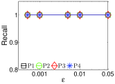
(a) recall vs. $\varepsilon$.

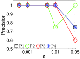
(b) precision vs. $\varepsilon$.

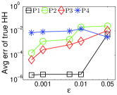
(c) err vs. $\varepsilon$.

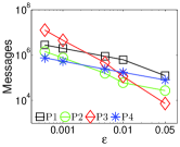
(d) msg vs. $\varepsilon$.

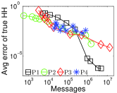
(e) err vs. msg

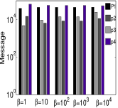
(f) msg vs. $\beta$.

Figure 1: Results for distributed weighted heavy hitters protocols on Zipfian distribution with skew=2.

6.1 Distributed Weighted Heavy Hitters

We denote four protocols for tracking distributed weighted heavy hitters as P1, P2, P3 and P4 respectively. As a baseline, we could send all $10^{7}$ stream elements to the coordinator, this would have no error. All of our heavy hitters protocols return an element $e$ as heavy hitter only if $\hat{W}_{e}/\hat{W}\geq\phi-\varepsilon/2$ while the exact weighted heavy hitter method which our protocols are compared against, returns $e$ as heavy hitter if $f_{e}(A)/W\geq\phi$.

We set the heavy-hitter threshold $\phi$ to $0.05$ and we varied error guarantee $\varepsilon$ in the range $\{5\times 10^{-4},10^{-3},5\times 10^{-3},$ $10^{-2},5\times 10^{-2}\}$. When the plots do not vary $\varepsilon$, we use the default value of $\varepsilon=10^{-3}$. Also we varied number of sites ($m$) from $10$ to $100$, otherwise we have as default $m=50$.

All four algorithms prove to be highly effective in estimating weighted heavy hitters accurately, as shown in recall (Figure 1(a)) and precision (Figure 1(b)) plots. In particular, the recall values for all algorithms are constant $1.0$.

Note that precision values dip, but this is because the true heavy hitters have $f_{e}(A)/W$ above $\phi$ where our algorithms only return a value if $\hat{W}_{e}/\hat{W}\geq\phi-\varepsilon/2$, so they return more false positives as $\varepsilon$ increases. For $\varepsilon$ smaller than $0.01$, all protocols have a precision of $1.0$.

When measuring (the measured) err as seen in Figure 1(c), our protocols consistently outperform the error parameter $\varepsilon$. The only exception is P4, which has slightly larger error than predicted for very small $\varepsilon$; recall this algorithm is randomized and has a constant probability of failure. P1 has almost no error for $\varepsilon=0.01$ and below; this can be explained by improved analysis for Misra-Gries [5] on skewed data, which applies to our Zipfian data. Protocols P2 and P3 also greatly underperform their guaranteed error.

The protocols are quite communication efficient, saving several orders of magnitude in communication as shown in Figure 1(d). For instance, all protocols use roughly $10^{5}$ messages at $\varepsilon=0.01$ out of $10^{7}$ total stream elements. To further understand different protocols, we tried to compare them by making them using (roughly) the same number of messages. This is achieved by using different $\varepsilon$ values. As shown in Figure 1(e); all protocols achieved excellent approximation quality, and the measured error drops quickly as we allocate more budget for the number of messages. In particular, P2 is the best if fewer than $10^{5}$ messages are acceptable with P3 also shown to be quite effective. P1 performs best if $10^{6}$ messages are acceptable.

In another experiment, we tuned all protocols to obtain (roughly) the same measured error of err = $0.1$ to compare their communication cost versus the upper bound on the element weights ($\beta$). Figure 1(f) shows that they are all robust to the parameter $\beta$; P2 or P3 performs the best.

6.2 Distributed Matrix Tracking

The strong results for distributed weighted heavy hitter protocols transfer over empirically to the results for distributed matrix tracking, but with slightly different trade-offs. Again, we denote our three protocols by P1, P2, and P3 in all plots. As a baseline, we consider two algorithms: they both send all data to the coordinator. One calls Frequent-Directions (FD)  [28], and second calls SVD which is optimal but not streaming. In all remaining experiments, we have used default value $\varepsilon=0.1$ and $m=50$, unless specified. Otherwise $\varepsilon$ varied in range $\{5\times 10^{-3},10^{-2},5\times 10^{-2},10^{-1},5\times 10^{-1}\}$, and $m$ varied in range $[10,100]$.

DataSet	PAMAP, $k=30$		MSD, $k=50$
Method	err	msg	err	msg
P1	7.5859e-06	628537	0.0057	300195
P2	0.0265	10178	0.0695	6362
P3wor	0.0057	3962	0.0189	3181
P3wr	0.0323	25555	0.0255	22964
FD	2.1207e-004	629250	0.0976	300000
SVD	1.9552e-006	629250	0.0057	300000

Table 1: Raw numbers of PAMAP and MSD.

Table 1 compares all algorithms, including SVD and FD to compute rank $k$ approximations of the matrices, with $k=30$ and $k=50$ on PAMAP and MSD respectively. Since err values for the two offline algorithms are minuscule for PAMAP, it indicates it is a low rank matrix (less than 30), where as MSD is high rank, since error remains, even with the best rank 50 approximation from the SVD method.

Note that P3wor and P3wr refer to Protocol 3, without replacement and with replacement sampling strategies, respectively. As predicted by the theoretical analysis, we see that P3wor outperforms P3wr in both settings, always having much less error and many fewer messages. Moreover, P3wor will gracefully shift to sending all data deterministically with no error as $\varepsilon$ becomes very small. Hence we only use P3wor elsewhere, labeled as just P3.

Also note that P1 in the matrix scenario is far less effective; although it achieves very small error, it sends as many messages (or more) as the naive algorithms. Little compression is taking place by FD at distributed sites before the squared norm threshold is reached.

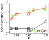
(a) err vs. $\varepsilon$.

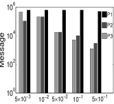
(b) msg vs. $\varepsilon$.

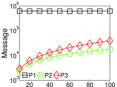
(c) msg vs. site

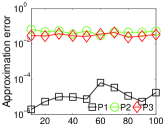
(d) err vs. site

Figure 2: Experiments for PAMAP dataset

Figures 2(a) and 3(a) show as $\varepsilon$ increases, error of protocols increases too. In case of P3  this observation is justified by the fact P3 samples $O((1/\varepsilon^{2})\log(1/\varepsilon))$ elements, and as $\varepsilon$ increases, it samples fewer elements, hence results in a weaker estimation of true heavy directions. In case of P2, as $\varepsilon$ increases, they allocate a larger error slack to each site and sites communicate less with the coordinator, leading to a coarse estimation. Note that again P1 vastly outperforms its error guarantees, this time likely explained via the improved analysis of Frequent-Directions [21].

Figures 2(b) and 3(b) show number of messages of each protocol vs. error guarantee $\varepsilon$. As we see, in large values of $\varepsilon$ (say for $\varepsilon>1/m=0.02$), P2 typically uses slightly more messages than P3. But as $\varepsilon$ decreases, P3 surpasses P2 in number of messages. This confirms the dependency of their asymptotic bound on $\varepsilon$ ($1/\varepsilon^{2}$ vs. $1/\varepsilon$). P1 generally sends much more messages than both P2 and P3.

Next, we examined the number of sites ($m$). Figures 2(c) and 3(c) show that P2 and P3 used more communication as $m$ increases, showing a linear trend with respect to $m$. P1 shows no trend since its communication depends solely on the total weight of the stream. Note that P1 sends its whole sketch, hence fix number of messages, whenever it reaches the threshold. As expected, the number of sites does not have significant impact on the measured approximation error in any protocol; see Figures 2(d) and 3(d).

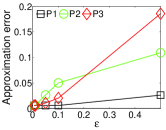
(a) err vs. $\varepsilon$.

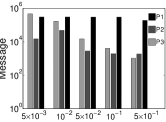
(b) msg vs. $\varepsilon$.

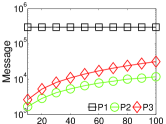
(c) msg vs. site

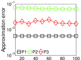
(d) err vs. site

Figure 3: Experiments for MSD dataset

We also compared the performance of protocols by tuning the $\varepsilon$ parameter to achieve (roughly) the same measured error. Figure 4 shows their communication cost (#msg) vs the err. As shown, protocols P1, P2, and P3 incur less error with more communication and each works better in various regimes of the err versus msg trade-off. P1 works the best when the smallest error is required, but more communication is permitted. Even though its communication is the same as the naive algorithms in these examples, it allows each site and the coordinator to run small space algorithms. For smaller communication requirements (several of orders of magnitude smaller than the naive methods), then either P2 or P3 are recommended. P2 is deterministic, but P3 is slightly easier to implement. Note that since MSD is high rank, and even the naive SVD or FD do not achieve really small error (e.g. $10^{-3}$), it is not surprising that our algorithms do not either.

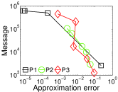
(a) PAMAP

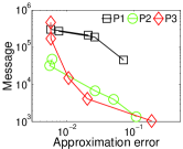
(b) MSD

Figure 4: Comparing the two protocols: msg vs. err

7 Conclusion

We provide the first protocols for monitoring weighted heavy hitters and matrices in a distributed stream. They are backed by theoretical bounds and large-scale experiments. Our results are based on important connections we establish between the two problems. Interesting open problems include, but are not limited to, extending our results to the sliding window model, and investigating distributed matrices that are column-wise distributed (i.e., each site reports values from a fixed column in a matrix).

Appendix A Proof of Lemma 4

Proof.

In order to reach round $j$ we must have $s$ items with priority $\rho_{n}>\tau_{j}=2^{j}$; this happens with probability $\min(1,w_{n}/2^{j})\leq\min(1,\beta/2^{j})\leq\beta/2^{j}$. We assume for now $\beta\leq 2^{j}$ for values of $j$ we consider; the other case is addressed at the end of the proof.

Let $X_{n,j}$ be a random variable that is $1$ if $\rho_{n}\geq\tau_{j}$ and $0$ otherwise. Let $M_{j}=\sum_{n=1}^{N}X_{n,j}$. Thus the expected number of items that have a priority greater than $\tau_{j}$ is $\textbf{{{E}}}[M_{j}]=\sum_{n=1}^{N}w_{n}/2^{j}\leq N\beta/2^{j}$. Setting $j_{N}=\lceil\log_{2}(\beta N/s)\rceil$ then $\textbf{{{E}}}[M_{j_{N}}]\leq s$.

We now want to use the following Chernoff bound on the $N$ independent random variables $X_{n,j}$ with $M=\sum_{n=1}^{N}X_{n,j}$ that bounds $\textbf{{{Pr}}}[M_{j}\geq(1+\alpha)\textbf{{{E}}}[M_{j}]]\leq\exp(-\alpha^{2}\textbf{{{E}}}[M_{j}]/(2+\alpha)).$

Note that $\textbf{{{E}}}[M_{j_{N}+1}]\leq(N\beta)/2^{j_{N}+1}\leq s/2$. Then setting $\alpha=1$ ensures that

$$(1+\alpha)\textbf{{{E}}}[M_{j_{N}+1}]=2\cdot(s/2)\leq s.$$

Thus we can solve

$$\textbf{{{Pr}}}[M_{j_{N}+1}\geq s] \leq\exp\left(-\frac{s/2}{3}\right)=\exp\left(-\frac{-s}{6}\right).$$

Thus since in order to reach round $j_{N}+1=\log_{2}(\beta N/s)+1=O(\log(\beta N/s))$, we need $s$ items to have priority greater than $\tau_{j_{N}+1}$, this happens with probability at most $e^{-\Omega(s)}$. Recall that to be able to ignore the case where $w_{n}>\tau_{j_{N}+1}$ we assumed that $\beta<\tau_{j_{N}+1}$. If this were not true, then $\beta>2^{\log_{2}(\beta N/s)+1}=2\beta N/s$ implies that $s>N$, in which case we would send all elements before the end of the first round, and the number of rounds is $1$. ∎

Appendix B Proof of Lemma 6

Proof.

To prove our claim, we use the following Chernoff-Hoeffding bound [35]. Given a set of negatively-correlated random variables $Y_{1},\ldots,Y_{r}$ and $Y=\sum_{n=1}^{r}Y_{n}$, where each $Y_{n}\in[a_{i},b_{i}]$, where $\Delta=\max_{n}(b_{n}-a_{n})$ then $\textbf{{{Pr}}}[|Y-\textbf{{{E}}}[Y]|\geq\alpha]\leq\exp(-2\alpha^{2}/r\Delta^{2})$.

For a given item $e\in[u]$ and any pair $(a_{n},w_{n})\in S$, we define a random variable $X_{n,e}$ as follows:

$$X_{n,e}=\bar{w}_{n}\textrm{ if }a_{n}=e,\textrm{ }0\textrm{ otherwise}.$$

Define a heavy set $H=\{a_{n}\in A\mid w_{n}\geq\tau_{j}\}$, these items are included in $S$ deterministically in round $j$. Let the light set be defined $L=A\setminus H$. Note that for each $a_{n}\in H$ that $X_{n,e}$ is deterministic, given $e$. For all $a_{n}\in S\cap L$, then $X_{n,e}\in[0,2\tau_{j}]$ and hence using these as random variables in the Chernoff-Hoeffding bound, we can set $\Delta=2\tau_{j}$.

Define $M_{e}=\sum_{a_{n}\in S}X_{n,e}$, and note that $f_{e}(S)=M_{e}$ is the estimate from $S^{\prime}$ of $f_{e}(A)$. Let $W_{L}=\sum_{a_{n}\in L}w_{i}$. Since all light elements are chosen with probability proportionally to their weight, then given an $X_{n,e}$ for $a_{i}\in S\cap L$ it has label $e$ with probability $f_{e}(L)/W_{L}$. And in general $\textbf{{{E}}}[\sum_{a_{n}\in S\cap L}\bar{w}_{n}]=\textbf{{{E}}}[W_{S\cap L}]=W_{L}$. Let $H_{e}=\{a_{n}\in H\mid a_{n}=e\}$. Now we can see

$$\textbf{{{E}}}[f_{e}(S)]=\textbf{{{E}}}\left[\sum_{n=1}^{|S|}X_{n,e}\right] =\sum_{a_{n}\in H_{e}}w_{n}+\textbf{{{E}}}\left[\sum_{a_{n}\in S\cap L}\tau_{j}\right]\cdot\frac{f_{e}(L)}{W_{L}}$$

$$=f_{e}(H)+W_{L}\cdot\frac{f_{e}(L)}{W_{L}}=f_{e}(A).$$

Now we can apply the Chernoff-Hoeffding bound.

$$\textbf{{{Pr}}}\left(\left|f_{e}(S)-f_{e}(A)\right|>\varepsilon W_{A}\right)=\textbf{{{Pr}}}\left(\left|M_{e}-E[M_{e}]\right|>\varepsilon W_{A}\right)$$

$$\leq\exp\left(\frac{-2\varepsilon^{2}W_{A}^{2}}{|S|4\tau_{j}^{2}}\right)\leq\exp\left(-\frac{1}{2}\varepsilon^{2}|S|/(1+\varepsilon)^{2}\right)\leq\delta,$$

where the last line follows since $(1+\varepsilon)W_{A}\geq\sum_{a_{n}\in S}\bar{w}_{n}\geq|S|\tau_{j}$, where the first inequality holds with high probability on $|S|$. Solving for $|S|$ yields $|S|\geq\frac{(1+\varepsilon)^{2}}{2\varepsilon^{2}}\ln(1/\delta)$. Setting $\delta=O(\varepsilon^{2}/\log(1/\varepsilon))=1/|S|$ allows the result to hold with probability at least $1-1/|S|$. ∎

Appendix C Distributed Matrix Tracking Protocol 4

Again treating each row $a_{i}$ as having weight $w_{i}=\|a_{i}\|^{2}$, then to mimic the weighted heavy-hitters protocol 4 we want to select each row with probability $\hat{p}=1-e^{-p\|a_{i}\|^{2}}$. Here $p=2\sqrt{m}/(\varepsilon\hat{F})$ represents the probability to send a weight $1$ item and $\hat{F}$ is a $2$-approximation of $\|A\|_{F}^{2}$ (i.e. $\hat{F}\leq\|A\|_{F}^{2}\leq 2\hat{F}$) and is maintained and provided by the coordinator. We then only want to send a message from the coordinator if that row is selected, and then it follows from the analysis in Section 4.3 that in total $O((\sqrt{m}/\varepsilon)\log(\beta N))$ messages are sent, since $O(\sqrt{m}/\varepsilon)$ messages are sent each round in between $\hat{F}$ doubling and being distributed by the coordinator, and there are $O(\log(\beta N))$ such rounds.

But replicating the approximation guarantees of protocol 4 is hard. In Algorithm 5, on each message a particular element $e$ has its count updated exactly with respect to a site $j$. Because of this, we only need to bound the expected weight of stream elements until another exact update is seen (at $1/p$) and then to compensate for this we increase this weight by $1/p$ so it has the right expected value. It also follows that the variances are bounded by $1/p^{2}$, and thus when $p$ is set $\Theta(\sqrt{m}/(\varepsilon W))$ we get at most $\varepsilon W$ error.

Thus the most critical part is to update the representation (of local matrices from $m$ sites) on the coordinator so it is exact for some query. We show that this can only be done for a limited set of queries (along certain singular vectors), provide an algorithm to do so, and then show that this is not sufficient for any approximation guarantees.

Replicated algorithm for matrices.

Each site can keep track of $A_{j}$ the exact matrix describing all of its data, and an approximate matrix $\hat{A}_{j}$. The matrix $\hat{A}_{j}$ will also be kept on the coordinator for each site. So the coordinator’s full approximation $\hat{A}=[\hat{A}_{1};\hat{A}_{2};\ldots;\hat{A}_{m}]$ is just the stacking of the approximation from each site. Since the coordinator can keep track of the contribution from each site separately, the sites can maintain $\hat{A}_{j}$ under the same process as the coordinator.

In more detail, both the site and the coordinator can maintain the $[U,\Sigma,V]={\textsf{svd}}(\hat{A}_{j})$, where $V=[v_{1},v_{2},\ldots,v_{d}]$ stores the right singular vectors and $\Sigma={\textsf{diag}}(s_{1},s_{2},\ldots,s_{d})$ are the singular values. (Recall, $U$ is just an orthogonal rotation, and does not change the squared norm.) Thus $\|\hat{A}_{j}x\|^{2}=\sum_{i=1}^{d}s_{i}^{2}\langle v_{i},x\rangle^{2}$. Now if we can consider setting $A^{\prime}=[\hat{A}_{j};r]$ where $\|r\|=\langle v_{i^{\prime}},r\rangle$, so it is along the direction of a singular vector $v_{i^{\prime}}$, then

$$\|A^{\prime}x\|^{2}=\|r\|^{2}\langle v_{i^{\prime}},x\rangle^{2}+\sum_{i=1}^{d}s_{i}^{2}\langle v_{i},x\rangle^{2}.$$

Thus if we update the singular value $s_{i^{\prime}}$ to $\bar{s}_{i^{\prime}}=\sqrt{s_{i^{\prime}}^{2}+\|r\|^{2}}$, (and to simplify notation $\bar{s}_{i}=s_{i}$ for $i\neq i^{\prime}$) then $\|A^{\prime}x\|^{2}=\sum_{i=1}^{d}(s^{\prime}_{i})^{2}\langle v_{i},x\rangle^{2}$. Hence, we can update the squared norm of $\hat{A}_{j}$ in a particular direction, as long as that direction is one of its right singular values. But unfortunately, in general, for arbitrary direction $x$ (if not along a right singular vector), we cannot do this update while also preserving or controlling the orthogonal components.

We can now explain how to use this form of update in a full protocol on both the site and the coordinator. The algorithm for the site is outlined in Algorithm 1. On an incoming row $a$, we updated $A_{j}=[A_{j};a]$ and send a message with probability $1-e^{-p\|a\|^{2}}$ where $p=2\sqrt{m}/(\varepsilon\hat{F})$. If we are sending a message, we first set $z_{i}=\sqrt{\|A_{j}v_{i}\|^{2}+1/p}$ for all $i\in[d]$, and send a vector $z=(z_{1},z_{2},\ldots,z_{d})$ to the coordinator. We next produce the new $\hat{A}_{j}$ on both site and coordinator as follows. Set $Z={\textsf{diag}}(z_{1},z_{2},\ldots,z_{d})$ and update $\hat{A}_{j}=ZV^{T}$. Now along any right singular vector $v_{i}$ of $\hat{A}_{j}$ we have $\|\hat{A}_{j}v_{i}\|^{2}=\|A_{j}v_{i}\|^{2}+1/p$. Importantly note that the right singular vectors of $\hat{A}_{j}$ do not change; although their singular values and hence ordering may change, the basis does not.

Algorithm 1 P4: Site $j$ process new row $a$

  Given $\hat{F}$ from coordinator, set $p=2\sqrt{m}/(\varepsilon\hat{F})$.

  The site also has maintained $[U,\Sigma,V]={\textsf{svd}}(\hat{A}_{j})$.

  Update $A_{j}=[A_{j};a]$.

  Set $\hat{p}=1-e^{-p\|a\|^{2}}$. Generate $u\in{\textsf{Unif}}[0,1]$.

  if ($u\leq\hat{p}$) then

     for $i\in[d]$ do $z_{i}=\sqrt{\|A_{j}v_{i}\|^{2}+1/p}$.

     Send vector $z=(z_{1},\ldots,z_{d})$.

     Set $Z={\textsf{diag}}(z_{1},\ldots,z_{d})$; update $\hat{A}_{j}=ZV^{T}$.

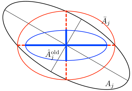
Figure 5: Possible update of $\hat{A}_{j}^{\text{old}}$ to $\bar{A}_{j}$ with respect to $A_{j}$ for $d=2$. Note the norm of a matrix along each direction $x$ is an ellipse, with the axes of the ellipse corresponding to the right singular vectors. Thus $\hat{A}_{j}^{\text{old}}$ and $\bar{A}_{j}$ have the same axes, and along those axes both $\bar{A}_{j}$ and $A_{j}$ have the same norm, but otherwise are incomparable.

Error analysis.

To understand the error analysis, we first consider a similar protocol, except where instead of each $z_{i}$, we set $\bar{z}_{i}=\|A_{j}v_{i}\|$ (without the $1/p$). Let $\bar{Z}={\textsf{diag}}(\bar{z}_{1},\ldots,\bar{z}_{d})$ and $\bar{A}_{j}=\bar{Z}V^{T}$. Now for all right singular vectors $\|A_{j}v_{i}\|^{2}=\|\bar{A}_{j}v_{i}\|^{2}$ (this is not true for general $x$ in place of $v_{i}$), and since $\bar{z}_{i}\geq s_{i}$ for all $i\in[d]$, then for all $x$ we have $\|\bar{A}_{j}x\|^{2}\geq\|\hat{A}_{j}^{\text{old}}x\|^{2}$, where $\hat{A}_{j}^{\text{old}}$ is the approximation before the update. See Figure 5 to illustrate these properties.

For directions $x$ that are right singular values of $\hat{A}_{j}$, this analysis should work, since $\|\bar{A}_{j}x\|^{2}=\|A_{j}x\|^{2}$. But two problems exist in other directions. First in any other direction $x$ the norms $\|A_{j}x\|$ and $\|\bar{A}_{j}x\|$ are incomparable, in some directions each is larger than the other. Second, there is no utility to change the right singular vectors of $\hat{A}_{j}$ to align with those of $A_{j}$. The skew between the two can be arbitrarily large, again see Figure 5, and without being able to adjust these, this error can not be bounded.

One option would be to after every $\sqrt{m}$ rounds send a Frequent Directions sketch $B_{j}$ of $A_{j}$ of size $O(1/\varepsilon)$ rows from each site to the coordinator. Then we use this $B_{j}$ as the new $\hat{A}_{j}$. This has two problems. First it only has $O(1/\varepsilon)$ singular vectors that are well-defined, so if there is increased squared norm in its null space, it is not well-defined how to update it. And second, still in between these updates within a round, there is no way to maintain the error.

One can also try to shorten a round to update when $\hat{F}$ increases by a $(1+\varepsilon)$ factor, to bound the change within a round. But this causes $O((1/\varepsilon)\log(\beta N))$ rounds, as in Section 5.2, and leads to $O((\sqrt{m}/\varepsilon^{2})\log(\beta N))$ total messages, which is as bad as the very conservative and deterministic algorithm P1. Thus, for direction $x$ that is a right singular value as analyzed above, we can get a Protocol 4 with $O((\sqrt{m}/\varepsilon)\log(\beta N))$ communication. But in the general case, how to, or if it is possible at all to, get $O((\sqrt{m}/\varepsilon)\log(\beta N))$ communication, as Protocol 4 does for weighted heavy hitters, in arbitrary distributed matrix tracking is an intriguing open problem.

Experiments with P4.

In order to give a taste on why P4 does not work, we compared it with other protocols. Figures 6 and 7 show the the error this protocol incurs on PAMAP and MSD datasets. Not only does it tend to accumulate error for smaller values of $\varepsilon$, but for the PAMAP dataset and small $\varepsilon$, the returned answer is almost all error.

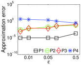
(a) err vs. $\varepsilon$.

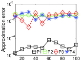
(b) err vs. site

Figure 6: P4 vs. other protocols on PAMAP

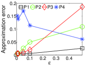
(a) err vs. $\varepsilon$.

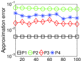
(b) err vs. site

Figure 7: P4 vs. other protocols on MSD

References

- [1] D. Achlioptas and F. McSherry. Fast computation of low rank matrix approximations. In STOC, 2001.
- [2] P. K. Agarwal, G. Cormode, Z. Huang, J. M. Phillips, Z. Wei, and K. Yi. Mergeable summaries. In PODS, 2012.
- [3] B. Babcock, S. Babu, M. Datar, R. Motwani, and J. Widom. Models and issues in data stream systems. In PODS, 2002.
- [4] B. Babcock and C. Olston. Distributed top-k monitoring. In SIGMOD, 2003.
- [5] R. Berinde, G. Cormode, P. Indyk, and M. Strauss. Space-optimal heavy hitters with strong error bounds. ACM Trans. Database Syst., 35(4), 2010.
- [6] T. Bertin-Mahieux, D. P. Ellis, B. Whitman, and P. Lamere. The million song dataset. In ISMIR, 2011.
- [7] M. Brand. Fast low-rank modifications of the thin singular value decomposition. Linear Algebra and its Applications, 415(1):20 – 30, 2006.
- [8] K. L. Clarkson and D. P. Woodruff. Numerical linear algebra in the streaming model. In STOC, 2009.
- [9] J. C. Corbett and et al. Spanner: Google’s globally distributed database. ACM TOCS, 31(3), 2013.
- [10] G. Cormode. The continuous distributed monitoring model. SIGMOD Record, 42, 2013.
- [11] G. Cormode and M. Garofalakis. Sketching streams through the net: Distributed approximate query tracking. In VLDB, 2005.
- [12] G. Cormode, M. Garofalakis, S. Muthukrishnan, and R. Rastogi. Holistic aggregates in a networked world: Distributed tracking of approximate quantiles. In SIGMOD, 2005.
- [13] G. Cormode and S. Muthukrishnan. An improved data stream summary: the count-min sketch and its applications. Journal of Algorithms, 55(1):58–75, 2005.
- [14] G. Cormode, S. Muthukrishnan, and K. Yi. Algorithms for distributed functional monitoring. TALG, 7(2):21, 2011.
- [15] G. Cormode, S. Muthukrishnan, K. Yi, and Q. Zhang. Continuous sampling from distributed streams. JACM, 59(2), 2012.
- [16] P. Drineas and R. Kannan. Pass efficient algorithms for approximating large matrices. In SODA, 2003.
- [17] P. Drineas, R. Kannan, and M. W. Mahoney. Fast Monte Carlo algorithms for matrices II: Computing a low-rank approximation to a matrix. SICOMP, 36(1):158–183, 2006.
- [18] N. Duffield, C. Lund, and M. Thorup. Priority sampling for estimation of arbitrary subset sums. JACM, 54(32), 2007.
- [19] A. Frieze, R. Kannan, and S. Vempala. Fast monte-carlo algorithms for finding low-rank approximations. JACM, 51(6):1025–1041, 2004.
- [20] R. Fuller and M. Kantardzic. FIDS: Monitoring frequent items over distributed data streams. In MLDM. 2007.
- [21] M. Ghashami and J. M. Phillips. Relative errors for deterministic low-rank matrix approximation. In SODA, 2014.
- [22] Z. Huang, K. Yi, and Q. Zhang. Randomized algorithms for tracking distributed count, frequencies, and ranks. In PODS, 2012.
- [23] G. Hulten, L. Spencer, and P. Domingos. Mining time-changing data streams. In KDD, 2001.
- [24] R. Y. Hung and H.-F. Ting. Finding heavy hitters over the sliding window of a weighted data stream. In LATIN. 2008.
- [25] R. Keralapura, G. Cormode, and J. Ramamirtham. Communication-efficient distributed monitoring of thresholded counts. In SIGMOD, 2006.
- [26] A. Lakhina, M. Crovella, and C. Diot. Diagnosing network-wide traffic anomalies. In SIGCOMM, 2004.
- [27] A. Lakhina, K. Papagiannaki, M. Crovella, C. Diot, E. D. Kolaczyk, and N. Taft. Structural analysis of network traffic flows. In SIGMETRICS, 2004.
- [28] E. Liberty. Simple and deterministic matrix sketching. In SIGKDD, 2013.
- [29] E. Liberty, F. Woolfe, P.-G. Martinsson, V. Rokhlin, and M. Tygert. Randomized algorithms for the low-rank approximation of matrices. PNAS, 104:20167–20172, 2007.
- [30] A. Manjhi, V. Shkapenyuk, K. Dhamdhere, and C. Olston. Finding (recently) frequent items in distributed data streams. In ICDE, 2005.
- [31] A. Metwally, D. Agrawal, and A. E. Abbadi. An integrated efficient solution for computing frequent and top-k elements in data streams. ACM TODS, 31(3):1095–1133, 2006.
- [32] J. Misra and D. Gries. Finding repeated elements. Sc. Comp. Prog., 2:143–152, 1982.
- [33] I. Mitliagkas, C. Caramanis, and P. Jain. Memory limited, streaming pca. In NIPS, 2013.
- [34] S. Muthukrishnan. Data streams: Algorithms and applications. Now Publishers Inc, 2005.
- [35] A. Panconesi and A. Srinivasan. Randomized distributed edge coloring via an extension of the chernoff-hoeffding bounds. SICOMP, 26:350–368, 1997.
- [36] S. Papadimitriou, J. Sun, and C. Faloutsos. Streaming pattern discovery in multiple time-series. In VLDB, 2005.
- [37] K. Papagiannaki, N. Taft, and A. Lakhina. A distributed approach to measure ip traffic matrices. In SIGCOMM IMC, 2004.
- [38] Z. Qian, X. Chen, N. Kang, M. Chen, Y. Yu, T. Moscibroda, and Z. Zhang. MadLINQ: large-scale distributed matrix computation for the cloud. In EuroSys, 2012.
- [39] V. Strumpen, H. Hoffmann, and A. Agarwal. A stream algorithm for the svd. Technical report, MIT, 2003.
- [40] M. Szegedy. The DLT priority sampling is essentially optimal. STOC, 2006.
- [41] S. Tirthapura and D. P. Woodruff. Optimal random sampling in distributed streams revisited. In PODC, 2011.
- [42] A. C.-C. Yao. Some complexity questions related to distributive computing. In STOC, 1979.
- [43] K. Yi and Q. Zhang. Optimal tracking of distributed heavy hitters and quantiles. Algorithmica, 65(1):206–223, 2013.