Validating Predictions of Unobserved Quantities

Abstract

The ultimate purpose of most computational models is to make predictions, commonly in support of some decision-making process (e.g., for design or operation of some system). The quantities that need to be predicted (the quantities of interest or QoIs) are generally not experimentally observable before the prediction, since otherwise no prediction would be needed. Assessing the validity of such extrapolative predictions, which is critical to informed decision-making, is challenging. In classical approaches to validation, model outputs for observed quantities are compared to observations to determine if they are consistent. By itself, this consistency only ensures that the model can predict the observed quantities under the conditions of the observations. This limitation dramatically reduces the utility of the validation effort for decision making because it implies nothing about predictions of unobserved QoIs or for scenarios outside of the range of observations. However, there is no agreement in the scientific community today regarding best practices for validation of extrapolative predictions made using computational models. The purpose of this paper is to propose and explore a validation and predictive assessment process that supports extrapolative predictions for models with known sources of error. The process includes stochastic modeling, calibration, validation, and predictive assessment phases where representations of known sources of uncertainty and error are built, informed, and tested. The proposed methodology is applied to an illustrative extrapolation problem involving a misspecified nonlinear oscillator.

1 Introduction and Motivation

Advances in computing hardware and algorithms in recent decades, along with accompanying advances in the fidelity of computational models, enable simulation of physical phenomena and systems of unprecedented complexity. This capability is revolutionizing engineering and science. For example, results of computational simulations are used heavily in the design of nearly all complex engineering systems, from consumer electronics to spacecraft and nuclear power plants. Furthermore, results of computational models are used to inform policy decisions in areas where the consequences of inaccurate predictions and poorly-informed decisions could be catastrophic, such as disaster response and climate change. However, for computational modeling to realize its full potential in such applications, it is critical that the reliability of the results of the models be systematically characterized. In the current paper, an approach to making such reliability assessments is proposed for a broad class of problems in computational science and engineering.

Any reliability assessment of a computational model must necessarily consider the purpose for which the model is to be used. A common use of computational models is to predict the response of some complex system and thereby to inform some decision regarding the system. For example, predictions from computational models might be used to decide which of several competing system designs will be superior, to decide whether a proposed use scenario for a system will meet operational objectives, or to decide how to respond to a system as it evolves. Typically, the decisions are informed by predictions of specific quantities describing the response of the system, these are the so-called quantities of interest (QoIs). An important feature of such uses of computational models is that observational data for the QoIs in the prediction scenario are not available, since otherwise the predictions would not be needed. This is the situation of interest here. There are of course other modes in which computational models are used in science and engineering, and in those cases the reliability issues will be different.

The assessment of reliability of computational models is often divided into three aspects: verification, validation and uncertainty quantification (collectively known as V&V-UQ). Verification is concerned with assessing the discrepancy between the computer simulation and the underlying mathematical model on which it is based. Uncertainty quantification is the process of assessing uncertainties that affect simulation predictions, such as those due to uncertain model inputs or inaccuracies in the model itself, and determining the resulting uncertainty in the QoIs. Finally, following [1, 3, 4], validation is the process of determining whether a mathematical model is a sufficient representation of reality for the purposes for which the model will be used; that is, for predicting specified QoIs to inform a specific decision. Thus, while verification is a purely mathematical process concerned only with the difference between computational and mathematical models, UQ and validation are concerned with the discrepancy between the mathematical model and the real world.

While verification is vitally important and sometimes overlooked in practice, it is largely understood [24, 18], with well developed techniques for estimating and controlling the impact of numerical errors on specified QoIs [2, 22]. In the remainder of this paper, it will be assumed that numerical solutions have been verified to ensure that numerical errors in the predictions are small compared to other sources of uncertainty, and so, verification will not be discussed further. Instead, we focus on the validation of and quantification of uncertainty in predictions of unobserved QoIs.

1.1 Validation Processes

In engineering practice, the “validity” of a computational model is often assessed by simply comparing the output of the model with experimental data. While such comparisons must be a part of any validity assessment, a straightforward process considering only the closeness of this comparison has two important shortcomings when used to assess the reliability of model predictions. First, it does not account for the uncertainties associated with the model or the data. Second, it precludes an assessment of the reliability of predictions in new situations or for unobserved quantities, which as discussed above, is the use we consider here. In essence, predictions are always extrapolations from available information, and the validation question is whether such extrapolation is justified.

In this context then, it is the validity of the prediction that is really of interest. We cannot speak of the validity of a model in general, since a model may produce valid predictions of some quantities in some circumstances, and not of others. This is different from the notion of validity of scientific theories, in which we insist that any inconsistency between a theory and observations falsifies the theory. In computational modeling, models known to be false in this strict scientific sense are used routinely (e.g., Newtonian mechanics), and the resulting predictions can nonetheless be valid, provided the inadequacies of the model have no significant effect on the prediction.

To address the shortcomings of naive comparisons with data as a technique for validating extrapolative predictions, a number of more sophisticated procedures have been proposed [25, 7, 19, 6, 23, 24, 18, 8, 13, 12, 17], and validation guidelines have been developed by professional engineering societies [1, 3, 4]. These have generally been positive developments, but they also have shortcomings. Most commonly, they do not directly address the validity of models to make predictions of unobserved QoIs. For instance, Higdon et al. [13] and Bayarri el al. [8] present similar validation frameworks for computational models, based on the work of Kennedy and O’Hagan on model calibration and model discrepancy representations [16]. These frameworks rely on statistical models—specifically Gaussian process models—to represent the difference between the model outputs and observational data. However, such representations are insufficient for validation of the ability to predict unobserved QoIs, because the discrepancy model is posed only for the observable quantities and there is generally no direct mapping from the observables to the QoIs.

A different approach in addressing the inadequacies in model structure is given by Strong et al. [26]. The main idea is to decompose the model into sub-functions and make judgments about the discrepancy of each sub-function. Strong et al. [26] propose a model refinement strategy based on sensitivity analysis to quantify the relative importance of different structural errors within a health economics model. The strategy of introducing discrepancy terms within the model at the source of the structural error is also embraced in the present paper. We leverage this technique to create a direct mapping between the discrepancy terms and both the observables and the unobserved QoIs. However, a number of challenges need to be addressed in using this approach for extrapolative predictions. First, since the discrepancy representation is a statistical model, it is highly dependent on calibration against observations and, hence, should not be used in situations in which it cannot be trained and tested. Thus, in general, use of this sort of discrepancy model in extrapolative predictions is suspect. Unlike Strong et al. [26] which use this strategy to guide model refinements based solely on building discrepancy models on prior knowledge, for our physics-based extrapolation problem we introduce a systematic calibration, validation and predictive assessment of these discrepancy terms to build confidence in their predictive capability. Furthermore, since there is no unique decomposition of the model, identifying the sources of error remains an issue. In our approach, we leverage the fact that the models are physics-based. Such models are generally constructed from highly reliable physical theories coupled with less reliable models to close the governing equations. This structure gives us a unique view of the modeling error. Since modeling errors are introduced entirely through the empirical models, we only need to introduce discrepancy terms where these embedded empirical models enter the formulation.

In pioneering work by Babuška et al [6], the impact of model discrepancy on unobserved QoIs was accounted for in the validation process. They addressed a structural mechanics problem in which the primary modeling challenge was the statistical representation of the unknown, spatially varying elastic modulus. In this case, it was expected that the statistical model could be calibrated to be consistent with observations from each of several available experimental scenarios, but that these separate calibrations need not be consistent with each other. The validation question in this case, was whether any such calibration discrepancies were important to the prediction of the QoI. This was tested by comparing the predictions arising from the different calibrations. This approach can be generalized to other problems in which the model parameterization is sufficiently rich that the model can always be adjusted to fit data from a single experimental scenario [20, 17, 21]. While this was true for the problem and models investigated by Babuška et al, with many engineering models this is not the case. Indeed, a common symptom of model inadequacy is that a model cannot be calibrated to match experimental data within experimental uncertainty, even for a single experimental scenario. In such cases, the Babuška et al validation approach is not able to account for the impact of these discrepancies on the QoIs, and thus, a more general formulation is needed.

1.2 Predictive Validation

As discussed above, there are currently no established techniques for assessing the validity of predictions of unobserved QoIs. Here we address this problem by proposing a process we call “predictive validation” by which it is possible to test the validity of such extrapolative predictions in a broad class of problems. In defining predictive validation, we will also specify the model characteristics that enable reliable predictions, a set of necessary conditions for extrapolative predictions and processes that allow satisfaction of these necessary conditions to be tested.

The predictive validation process described here was developed to evaluate predictions regarding physical systems. Such systems are commonly described by models based on highly reliable theory (e.g., conservation laws), whose validity is not in question in the context of the predictions to be made. However, these highly reliable theories typically must be augmented with one or more “embedded models,” which are less reliable. The less reliable embedded models may embody various modeling approximations, empirical correlations, or even direct interpolation of data. For example, in continuum mechanics, the embedded models might include constitutive models and boundary conditions, while in molecular dynamics they would include models for interatomic potentials. We will refer to such models—i.e., highly-fidelity models with lower-fidelity embedded components—as composite models.

The fact that the composite models used for prediction are built on highly reliable models is an important ingredient enabling reliable extrapolation in the approach described here, even though less reliable embedded models are also used. Specifically, we require that the less reliable models are not used outside the range where they have been calibrated and tested. This restriction does not necessarily limit our ability to extrapolate using the composite model since the relevant scenario space for each embedded model is specific to that embedded model, not the composite model in which it is embedded.

Another important ingredient is a representation of the uncertainty. We require mathematical representations of existing or prior information, the uncertainty in the observational data that will be used to inform and test the model, and the uncertainty in model predictions resulting from model inadequacy. Since Bayesian probability [11, 15, 27] provides a powerful representation of uncertainty, probabilistic models are used to describe uncertainty in this work, and the development of these probabilistic models is the first step of the predictive validation process. In particular, as in previous work [16, 13, 8], our approach relies heavily on statistical models of model discrepancy. However, unlike previous work, we take advantage of the structure of the composite model described above to introduce discrepancy models that can be used to evaluate uncertainty in unobserved quantities. This advance is accomplished by posing a model for the error in the embedded physical model directly, rather than a model for the discrepancy between observations and the model output for the observables.

Prior information on parameters and experimental uncertainty is also represented using Bayesian probabilistic models. In this way, we strive to account for all significant sources of uncertainty, including uncertainty in model inputs (e.g., parameters and boundary conditions), model errors, and observational data; so that the uncertainties in any model output, whether observed or unobserved, are represented. The original composite model plus these uncertainty models provides a complete model representing both our knowledge of the physics as well as important sources of uncertainty. This complete model is then the subject of the predictive validation process.

Typically, both the embedded physical models and the accompanying uncertainty models have parameters that must be determined from observations through calibration. In our approach, calibration is the first in an integrated, three-step process for assessing the reliability of extrapolative predictions issued by the complete model described above. The three steps—calibration, validation, and predictive assessment—are designed to answer three distinct questions regarding the model and its predictive capability. In calibration, the model is informed by data. Specifically, parameter values and their uncertainties are inferred from available observations by solving an inverse problem. The use of probability to represent uncertainty naturally leads to the formulation of the calibration problem as a Bayesian update.

In validation, outputs from the calibrated model are checked for consistency with available observations. While this consistency is not sufficient for predictive validation, it is necessary. Unlike calibration, the validation step is not naturally expressed in the language of Bayesian hypothesis testing because there are not well-defined alternative hypotheses. Instead, we must assess whether the validation data are plausible according to the model. There are a number of possibilities for quantifying this plausibility. Here we use highest posterior density credible sets.

Finally, predictive assessment determines whether the calibration and validation phases were sufficiently informative and challenging to provide confidence in the reliability of the predictions of the QoIs. Specifically, one must answer a number of questions about what the validation tests imply about the QoI predictions. This assessment relies on sensitivity analysis along with knowledge about the embedded models and their formulation.

Notice that in this approach to predictive validation, calibration and validation are based primarily on statistical analysis. However, all representations of uncertainty (e.g., models of uncertainty due to model discrepancy) depend heavily on the structure of the physical model and knowledge about the physical system being modeled. This knowledge is also crucial to the predictive assessment. It is this reliance on knowledge of and reliable theory about the physical system being modeled that makes extrapolative prediction possible.

The remainder of the paper is organized as follows. Important features of a composite model and associated uncertainty representations that enable predictive validation for unobserved QoIs are described abstractly in §2. Specific procedures used to assess the model and build confidence in its predictive capability is introduced in §3. The main ideas and tools of the predictive validation approach are illustrated using a simple example involving extrapolative predictions made for a spring-mass-damper system in §4. Concluding remarks in §5 address the practical challenges in carrying out the proposed validation processes for real-world applications.

2 Model Inadequacy and Discrepancy Representations in Predictive Validation

In developing the predictive validation process to be described, it is important to be precise about what constitutes a prediction. Here, a prediction is the result of a computational simulation conducted to compute specific QoIs which are to be used to support some decision regarding the system being simulated. Further, there is no observational data available for the QoIs for the scenarios of interest, since otherwise predictions would not be necessary. Thus, the credibility of the prediction must established based on available data for other quantities and/or scenarios, along with any other available information about the system. The fundamental challenge is to make credible predictions, despite the fact that the predictions are extrapolations from available information. Furthermore, in recognition of the fact that observational data have uncertainties, and that models are imperfect, we insist that predictions must be endowed with characterized uncertainties.

In general, the need to extrapolate raises concerns about the reliability of the predictions, and, indeed, we must ask: “what entitles us to make such predictions?” Part of the answer is that, unlike purely empirical models that can be used solely to represent observations, the models used to predict the behavior of physical systems are often based on theories that are known to be highly reliable within well-defined domains of applicability. However, these highly reliable theories are usually augmented with one or more “embedded models,” which are less reliable. Thus, the model as a whole is a composite model, as defined in §1. In the predictive validation approach proposed here, reliable predictions are enabled by the reliable theories that form the foundation of the composite model, whose validity in the prediction scenario is not in doubt.

To make these ideas clear, a simple abstract prediction problem is presented in §2.1. This is the simplest problem that has the characteristics of prediction discussed above. Critical to the prediction validation process is the representation of uncertainty due to the imperfections of the model. Background on such discrepancy representations is provided in §2.2, and discrepancy modeling for predictive validation is described in §2.3. Finally, generalizations of the abstract problem described in §2.1 to encompass predictions in complex physical systems are discussed in §2.4.

2.1 Abstract Problem Statement

Reliable predictions are enabled by the use of reliable physical theory whose validity in the context of the predictions to be made is not in doubt. Let this theory be written mathematically as

$$\mathcal{R}(u,\tau;r)=0,$$ (1)

where $\mathcal{R}$ is an operator expressing the theory. For example, in continuum mechanics, $\mathcal{R}$ would be a partial differential operator expressing conservation of mass, momentum, and energy. In this formulation, $u$ is the solution or state variable, and $r$ is a set of scenario variables needed to precisely define the problem being considered. The scenario variables might include the geometry of the solution domain, boundary conditions, and other parameters that define the problem. The final variable $\tau$ is a quantity that needs to be known to solve (1). For example, in continuum mechanics, $\tau$ could be the strain energy or the stress tensor.

If $\tau$ were known in terms of $u$ and $r$, the system would be closed, and (1) would implicitly define a mapping from the scenario variables $r$ to the solution variables $u$. However, it is often the case that the required relationship between $\tau$ and $u$ and $r$ is unknown or does not exist—i.e., $u$ and $r$ do not fully define $\tau$. In either case, a model, which we call an embedded model, is required, and is written $\tau_{m}$:

$$\tau\approx\tau_{m}(u;s,\theta),$$ (2)

where $\approx$ indicates that the model is imperfect; $s$ is a set of scenario variables for the embedded model; and $\theta$ is a set of parameters required by the model in addition to the scenario. These are the calibration or tuning parameters for the model. Note that the scenario space of the embedded model may be different from that of the global model in which it is embedded, so that $r$ and $s$ are not necessarily the same. In particular, $s$ often includes only a subset of the variables of $r$. Further, in many settings, $\tau_{m}$ is formulated entirely in terms of the local solution $u$ and calibration parameters $\theta$, in which case $s$ is empty. The fact that the scenario spaces of the global composite model and the embedded model are different is an important feature enabling reliable extrapolative predictions.

For the purposes of model calibration and validation, we require that some observable quantities $y$ can be measured experimentally. These observable quantities are different from the prediction QoIs $q$, but both $y$ and $q$ are determined from the model state, the scenario, and possibly the embedded model:

$$y=\mathcal{Y}(u,\tau;r),$$ (3)

$$q=\mathcal{Q}(u,\tau;r),$$ (4)

where, for simplicity of exposition, the theories underlying the operators $\mathcal{Y}$ and $\mathcal{Q}$ are presumed to be as reliable as the models embodied by $\mathcal{R}$.

2.2 Background on Model Discrepancy

In general, the model $\tau_{m}$ is less reliable than the model in which it is embedded either because its dependencies or functional form are incorrect (structural inadequacy/uncertainty) or because the parameters $\theta$ are not perfectly known (parameter error/uncertainty) or both. These errors introduce error in the model and, in turn, in both the solution and the QoI. In their seminal paper, Kennedy and O’Hagan [16] address this fact by introducing a statistical model for “the difference between the true value of the real world process and the code output at the true values of the inputs”. In their approach, which has become very common in the Bayesian literature [13, 8], this statistical model is posed directly for the observable quantities, such that (3) is replaced by

$$y=\mathcal{Y}(u,\tau_{m};r)+\delta_{y}(r;\alpha),$$

where $\delta_{y}$ is the model for the uncertainty in the observables induced by structural inadequacy, and $\alpha$ are a set of hyperparameters for that model, while $u$ is still determined by the original composite model $\mathcal{R}(u,\tau_{m};r)=0$.

In the present context, this treatment of the error is incomplete because it says nothing about the effect of model discrepancy on the QoIs. An analogous formulation for the QoIs is

$$q=\mathcal{Q}(u,\tau_{m};r)+\delta_{q}(r;\beta),$$

and thus, the full model is given by

$$\mathcal{R}(u,\tau_{m};r)=0,$$ (5)

$$y=\mathcal{Y}(u,\tau_{m};r)+\delta_{y}(r;\alpha),$$ (6)

$$q=\mathcal{Q}(u,\tau_{m};r)+\delta_{q}(r;\beta).$$ (7)

Here, the hyperparameters $\alpha$ and $\beta$ need to be calibrated, as well as the parameters of $\tau_{m}$, $\theta$. In the Kennedy and O’Hagan approach, the calibration of $\theta$ and $\alpha$ would be performed together using data for the observable $y$. But, because data for the QoIs $q$ are not available, this approach cannot be used to calibrate the hyperparameters $\beta$. Furthermore, even if one were able to pose a model $\delta_{q}$ that did not require calibration, there would be no way to test this model in the validation process, making it inappropriate for use in predictions. Clearly, a different approach is needed. Here we propose to take advantage of the structure of the composite model to introduce model uncertainty representations that can be informed and tested using data as well as used to quantify the uncertainty in predictions of the QoIs.

2.3 Discrepancy Modeling for Predictive Validation

The point of predictive validation is to assess the predictive capability of the model—i.e., to characterize the accuracy of the predictions of $q$. A key challenge in this process is to determine what the observed discrepancies between the model outputs and observational data imply about the reliability of the QoI predictions. In the formulation of §2.2, one must infer $\delta_{q}$ from observations of $y$. In general, this inference is extremely challenging because there is no direct mapping from the observables to the QoIs—i.e., given only $y$, one cannot evaluate $q$. Thus $\delta_{q}$ cannot be constructed directly from the physical model and the observations alone. Additional modeling assumptions are required.

Alternatively, in the predictive validation process, a mathematical relationship between the observables and the QoIs is constructed by formulating uncertainty models to represent errors at their sources. Such models are able to provide uncertain predictions for both the observables and the QoIs without additional assumptions. Thus, observational data can be used to inform and test these uncertainty models, and that information can directly influence the predictions of the QoIs.

To accomplish this, we recognize that the sole source of the modeling error in the current example is the embedded model $\tau_{m}$. Thus, instead of modeling the effects of this error on the observables and QoIs separately as in §2.2, we enrich the embedded physical model (2) with a model that represents not only the physics of the original model but also the uncertainty introduced by the structural inadequacy of that model. For example, one could write

$$\tau\approx\tau_{m}(u,s;\theta)+\epsilon_{m}(u,s;\alpha),$$

where $\epsilon_{m}$ denotes the uncertainty representation, which may depend on additional parameters $\alpha$. Given our choice to use probability to represent uncertainty, it is natural that $\epsilon_{m}$ is a stochastic model, even when the physical phenomenon being modeled is inherently deterministic. Of course, an additive model is not necessary; other choices are possible. More importantly, the form of $\epsilon_{m}$ must be determined. The specification of a stochastic model $\epsilon_{m}$ is driven by physical knowledge about the nature of error as well as practical considerations necessary to make computations with the model tractable. Although general principles for developing physics-based uncertainty models need to be developed, the specification of such a model is clearly problem-dependent and, thus, will not be discussed further here.

For the current purposes, it is sufficient to observe that the model $\epsilon_{m}$ is posed at the source of the structural inadequacy—i.e., in the embedded model for $\tau$. The combination of the physical and uncertainty models forms an enriched composite model, which takes the following form in the current case:

$$\mathcal{R}(u,\tau_{m}+\epsilon_{m};r)=0,$$ (8a)

$$y=\mathcal{Y}(u,\tau_{m}+\epsilon_{m};r),$$ (8b)

$$q=\mathcal{Q}(u,\tau_{m}+\epsilon_{m};r).$$ (8c)

The inadequacy model, $\epsilon_{m}$, appears naturally in the calculation of both $y$ and $q$, both directly through the possible dependence of $\mathcal{Y}$ and $\mathcal{Q}$ on $\tau$, and indirectly via the dependence of $u$ on $\tau$ through $\mathcal{R}$. The structural uncertainty can therefore be propagated to both the observables and the QoIs. Furthermore, one can learn about $\epsilon_{m}$—i.e., inform and test the model—from data on the observables and then transfer that knowledge to the prediction of the QoIs. The predictive validation process described in §3 is designed to address prediction problems of this type. The process involves training (calibration) embedded models and their inadequacy models, testing (validation) the embedded model and its use in the enriched composite model (8), and assessing (predictive assessment) whether the knowledge gained through these processes can be reliably transferred to the QoI predictions.

2.4 Generalized Problem Abstraction for Complex Systems

The abstract problem statement from §2.1 was designed as a simple illustrative example of a broad class of problems in which validated predictions of unobserved quantities are needed. This simple formulation can be generalized in a number of ways to encompass most computational prediction problems in science and engineering, including predictions in complex physical systems, in which many interacting physical phenomena are at work. These generalizations are discussed here.

The first generalization is that many unreliable embedded models of different phenomena may be required to represent the system being studied. For example, in a combustion problem, models for thermodynamics, molecular transport, radiation transport, and chemical reactions may need to be embedded in the equations for the conservation of mass, momentum and energy. To represent this situation, we introduce a set of $N$ quantities $\tau_{i}$ for $1\leq i\leq N$ which need to be modeled to close the governing equations:

$$\mathcal{R}(u,\tau_{1},\tau_{2},\ldots,\tau_{N};r)=0.$$ (9)

An embedded model for each of these quantities would then be needed, each of which could have a set of calibration parameters $\theta_{i}$, a set of model-specific scenario parameters $s_{i}$, and an inadequacy representation $\epsilon_{im}$ with hyperparameters $\alpha_{i}$:

$$\tau_{i}\approx\tau_{im}(u;\theta_{i},s_{i})+\epsilon_{im}(u;\alpha_{i},s_{i}).$$ (10)

The second generalization is that the experimental situation in which observations are made may be so different from the prediction situation that it is represented by a different reliable model $\cal R$. This experimental scenario might also depend on a number of new quantities $\tau$ that must be modeled. For example, these might represent the response of the measuring instrument or some characteristic of the experimental apparatus. In this case, the experimental scenario may be described by different parameters than the prediction scenario. There will in general be some number $N_{e}$ of different experiments, each of which involves a set of modeled quantities particular to the experiment as well as at least one of the modeled quantities used in predictions. To provide the most direct information regarding the embedded models used in the predictions, each of the experimental scenarios used for calibration would involve only one of the embedded models used for prediction and a minimum number of additional embedded models required to simulate the experiment (ideally none).

This situation can be formalized by introducing $N_{e}$ theoretical descriptions $\mathcal{R}^{i}$, where the superscript is the experiment index. Each of these models depends on a set $\{\tau\}^{i}$ of the embedded models used for prediction, with elements $\tau^{i}_{j}=\tau_{k}$ for some $k$, and a set of additional embedded models necessary for the experiment, denoted by $\{\sigma\}^{i}$ with elements $\sigma^{i}_{j}$. Furthermore, each of the experiments will in general involve a different observation model $\mathcal{Y}^{i}$. The experiments to be used for calibration and validation can therefore be expressed:

$$0 = \mathcal{R}^{i}(u^{i},\{\tau\}^{i},\{\sigma\}^{i};r^{i})\qquad 1\leq i\leq N_{e}$$ (11)

$$y^{i} = \mathcal{Y}^{i}(u^{i},\{\tau\}^{i},\{\sigma\}^{i};r^{i})\qquad 1\leq i\leq N_{e}$$ (12)

where $u^{i}$ denotes the state variables, $y^{i}$ is the vectors of observation data, and $r^{i}$ is the vector of scenario parameters for experiment $i$.

Each of the prediction modeled quantities $\tau_{k}$ has been modeled as $\tau_{km}+\epsilon_{km}$ for use in the prediction, as discussed above, so each vector of prediction modeled quantities $\{\tau\}^{i}$ is associated with a vector of models $\{\tau_{m}\}^{i}$ and a vector of error models $\{\epsilon_{m}\}^{i}$. In addition, models for the experimental modeled quantities $\sigma$ must be posed. For each experiment $i$, there is thus a vector of models $\{\sigma_{m}\}^{i}$, and each such model may have an associated error model, so there is generally a vector of error models $\{\delta_{m}\}^{i}$ for each experiment. These models will in general have parameters which must be determined from data, and their validity will need to be assessed as with the prediction models.

The final generalization arises because the state variables $u^{i}$ associated with model $\mathcal{R}^{i}$ for the various experiments need not be the same, or consistent with the state variables $u$ for the prediction model. For example, in a fluid dynamics problem, the prediction state variables would generally be a three-dimensional vector field, while in the model for the viscometer in which the parameter in the constitutive model for the internal stress (the viscosity) is determined, the state variable is a one-dimension function for the azimuthal velocity. Thus while the same embedded model is applied in both the prediction and the experiment, the dependence of the embedded model on the state must be different. We can express this by defining arguments $v_{k}$ for each embedded model that are consistent for the prediction and all experiments. An operator $\mathcal{V}^{i}_{k}$ is needed that maps the state variable for each scenario to the argument of the model $\tau_{km}$.

With these generalizations, the abstract statement of the prediction problem, analogous to (8) is

$$0 = \mathcal{R}(u,\{\tau_{m}\}^{0}+\{\epsilon_{m}\}^{0},r)$$ (13)

$$q = \mathcal{Q}(u,\{\tau_{m}\}^{0}+\{\epsilon_{m}\}^{0},r)$$ (14)

$$0 = \mathcal{R}^{i}(u^{i},\{\tau_{m}\}^{i}+\{\epsilon_{m}\}^{i},\{\sigma_{m}\}^{i}+\{\delta_{m}\}^{i},r^{i})\qquad\mbox{for $1\leq i\leq N_{e}$}$$ (15)

$$y^{i} = \mathcal{Y}^{i}(u^{i},\{\tau_{m}\}^{i}+\{\epsilon_{m}\}^{i},\{\sigma_{m}\}^{i}+\{\delta_{m}\}^{i},r^{i})\qquad\mbox{for $1\leq i\leq N_{e}$}$$ (16)

where the embedded models appearing in composite model of the prediction have the form:

$$\tau_{k}\approx\tau_{km}(\mathcal{V}_{k}(u),\theta_{k},s_{k})+\epsilon_{km}(\mathcal{V}_{k}(u),\alpha_{k},s_{k})$$ (17)

while when the same models appear in the composite model for experiment $i$ they have the form:

$$\tau_{k}\approx\tau_{km}(\mathcal{V}^{i}_{k}(u),\theta_{k},s_{k})+\epsilon_{km}(\mathcal{V}^{i}_{k}(u),\alpha_{k},s_{k}).$$ (18)

Clearly, if the experiments are to provide any meaningful information about the prediction models, then the errors and uncertainties associated with the embedded models for $\{\sigma\}^{i}$ will have to be sufficiently small, or ideally entirely absent. That is, it is preferable if there are no extra modeled quantities in the composite model for the experiment. Similarly, as mentioned above, experiments in which only one of the embedded models is exercised are particularly valuable for learning about that model, since it avoids confounding uncertainties from other models. Experiments that exercise many embedded models are generally not as useful for calibrating embedded models.

This fact leads to the idea of a validation pyramid[5]. In particular, it is helpful to organize the experimental inputs to the simulation of a complex system hierarchically. At the lowest level of the hierarchy are simple experiments that exercise only one, or few embedded models. Such experiments are generally relatively inexpensive, relatively well controlled and numerous. They therefore can provide abundant well characterized data, which is ideal for the calibration of embedded models. These experiments are at the base of the pyramid. As one ascends the hierarchy, or pyramid, the experiments exercise more of the embedded models; they become increasingly expensive, and they commonly become more difficult to control and instrument. Data from these more complex experiments are thus more limited and are often of lower quality, that is, they have higher uncertainty. For these reasons, the higher experiments are in the hierarchy, the less useful they are for calibrating embedded models. They are, however, critical for validation testing. At the highest level of the pyramid are experiments conducted on systems with complexity similar or identical to the system of interest. Experiments on the system of interest are particularly valuable because they provide an opportunity to detect unanticipated and therefore unmodeled phenomena.

The generalizations discussed above are important to understanding how the predictive validation process discussed here applies to the simulation of complex systems. However, the basic ideas underlying predictive validation are more easily discussed in the context of simpler examples, which are well characterized by the simple abstract problem described in §2.1. Therefore, the generalizations described above will not be discussed further.

3 Predictive Validation Processes

Given a composite model like (8), there are likely to be parameters—e.g., $\theta$ and $\alpha$ in $\tau_{m}$ and $\epsilon_{m}$, respectively, from §2.3—that must be determined from observations (calibration). If the inadequacy model $\epsilon_{m}$ faithfully represents the discrepancies between the model for the observables $\mathcal{Y}$ and the observations (validation), we then use it in the model for the QoIs $\mathcal{Q}$ to predict how the observed discrepancies impact uncertainty in the QoI, and assess the adequacy of the calibration and validation processes for the QoI prediction (predictive assessment). Thus, the process needed to assess the accuracy and credibility of the predictions involves three activities: calibration, validation, and predictive assessment. These activities are described briefly below.

3.1 Model Calibration

The parameters in the embedded models $\tau_{m}$ and inadequacy models $\epsilon_{m}$ need to be specified in some way. Some parameters may be very well known, with either known or negligible uncertainties, and such parameters need not be calibrated (e.g., the speed of light or the acceleration due to gravity on Earth). However, in most cases, at least some of the parameters are not well-known, and so values must be determined that are consistent with existing knowledge about the phenomenon and with observational data. Generally, this can be posed as an inverse problem, where the model inputs are be determined by requiring the from the model outputs to match observations under constraints imposed by prior knowledge. Furthermore, the uncertainties in the data being used and the qualitative and often imprecise nature of existing knowledge about the parameters must be accounted for to yield estimates of the resulting uncertainty in the calibrated parameters.

There are a number of different approaches that might be formulated to solve such inverse problems [9]. Provided they produce consistent estimates and uncertainties for the parameters, they can serve as calibration techniques for the predictive validation approach discussed here. Recall, however, that we have selected Bayesian probability for our mathematical representation of uncertainty. In this context, a very natural and powerful approach to calibration is Bayesian inference, which relies on Bayes’ theorem:

$$p(\theta,\alpha|Y,I)=\frac{p(\theta,\alpha|I)L(\theta,\alpha;Y,I)}{\int p(\theta,\alpha|I)L(\theta,\alpha;Y,I)\,d\theta d\alpha}$$ (19)

where $Y$ represents the calibration data, and $p(\cdot|\cdot)$ is a conditional probability density function (PDF). Here, $p(\theta,\alpha|I)$ is the joint prior PDF of the parameters $\theta$ and $\alpha$, which is conditional on the prior knowledge $I$. The function $L(\theta,\alpha;Y,I)$ is the likelihood, which is given by:

$$L(\theta,\alpha;Y,I)=p(y=Y|\theta,\alpha,I).$$ (20)

It represents the likelihood of observing the data given the model and its uncertainty, the particular values of $\theta$ and $\alpha$, and the uncertainty in the measurements. Finally, $p(\theta,\alpha|Y,I)$ is the posterior PDF, the joint distribution of the parameters, conditioned on both the data and the prior knowledge. This posterior PDF is the Bayesian solution of the inverse problem, representing the desired estimate of the parameters, with uncertainties.

3.2 Validation

Calibrating the model does not guarantee that its outputs will be consistent with the calibration data, much less new data not used for calibration. Indeed, calibration can only ensure that the model matches the calibration data as well as possible, which may not be very well at all. It is therefore necessary that consistency of model outputs with the experimental observations be explicitly checked. This process of comparing models to observations is consistent with the classical notion of validation. However, in making such comparisons, determining how much discrepancy between model and observations is acceptable is subtle and important. The most relevant metric is the implied discrepancy in the QoI (i.e., the difference between the predicted QoI and reality), but this metric is inaccessible in standard validation approaches. Hence, the determination of a tolerance is generally left to expert opinion [18].

However, the consideration of uncertainties provides a natural way to define the acceptable level of discrepancy. It is simply that the data must be a plausible outcome of the model, with all its uncertainties, including those due to the model inputs, observational errors, and model inadequacy. This simply tests whether the uncertainty models, particularly the inadequacy model, can plausibly account for the causes of the discrepancies. If any of the available data, including data used for calibration as well as that intended only for validation, is not a plausible outcome of the model with its uncertainties, then we can conclude that the uncertainty representations are somehow insufficient and should not be used for prediction.

It remains then to define what it means for the data to be a plausible outcome of the model. This clearly depends on how uncertainties are being represented mathematically. If one represents uncertainty using probability, as we do here, then the validation criterion will clearly need to be that the data is not too improbable. To quantify this we require a metric and a tolerance.

Given the probability distributions for the model inputs $\theta$ and $\alpha$ obtained from the calibration process, the model (8) yields a probability density for each individual observable quantity $y_{i}$, $p(y_{i}|Y,I)$. This probability density is formally conditional on all the calibration data and our prior knowledge, due to the calibration process, and it is helpful to explicitly acknowledge this fact, as is done here. Let an observational datum for observable $y_{i}$ be $Y_{i}$, then a useful approach to determine whether the datum is a plausible outcome of the model can be based on Bayesian credible intervals, of which several can be defined.

Particularly appropriate for our use are highest posterior density (HPD) credibility intervals [10]. The $\beta$-HPD $(0\leq\beta\leq 1)$ interval is an interval or a set of intervals for which the probability of belonging to it is $\beta$ and the probability density of all the points in the interval is greater than the density of the points outside the interval. However, because HPD credibility sets are defined in terms of the probability density, they are not invariant to a change of variables. This is particularly undesirable when formulating a validation metric because it means that one’s conclusions about model validity would depend on the arbitrary choice of variables (e.g., whether one considers the observable to be the frequency or the period of an oscilation). To avoid this problem, we introduce a modification of the HPD in which the credible set is defined in terms of the probability density relative to a specified distribution $q$. An appropriate definition of $q$ would be the ignorance distribution [15] on the data space. Using this definition of the highest posterior relative density (HPRD), a credibility metric can be defined as $\gamma=1-\beta_{\rm min}$, where $\beta_{\rm min}$ is the smallest value of $\beta$, for which the observation $Y_{i}$ is in the HPRD-credibility set for $y_{i}$. That is:

$$\gamma(Y_{i})=1-\int_{S}p(y_{i}|Y,X)\,dy_{i},\quad\mbox{where}\quad S=\left\{y_{i}:\frac{p(y_{i}|Y,X)}{q(y_{i})}\geq\frac{p(Y_{i}|Y,X)}{q(Y_{i})}\right\}$$ (21)

When $\gamma$ is smaller than some tolerance, say less than $0.05$ or $0.01$, the data are considered an implausible outcome of the model.

A validation metric based on HPRD credibility sets is proposed here because it seems to be best aligned with intuitive notions of agreement between the model predictions and observations, even for skewed and multi-modal distributions. For example, for multi-modal distributions, an HPRD region may consist of multiple disjoint intervals [14] around the peaks in the distribution, leaving out the low probability density regions between the peaks.

Even if all available data are credible outcomes of the model by an HPRD criterion, this does not imply that the model with its associated uncertainty is valid for predicting the QoIs. Indeed it only implies that we have so far failed to invalidate the model for use in making predictions. To determine the validity of a prediction, it is necessary to assess whether the validation tests have been sufficiently thorough to give confidence in the prediction, and whether, in the prediction scenario, all the embedded models are being used in regimes in which they are expected to be reliable. This is the role of predictive assessment.

3.3 Predictive Assessment

As discussed in §1, assessing the reliability of a prediction is difficult because prediction fundamentally requires extrapolation from available data. Such an extrapolation cannot be justified based on the agreement between the data and the model alone. Knowledge about the structure of the physical and uncertainty models and their potential shortcomings is important to determining whether the validation tests that have been performed are sufficient to warrant confidence in the predictions. There are two primary questions that need to be addressed. The first is whether the QoIs are sensitive to aspects of the embedded models that have not been effectively informed by the calibration and tested through the validation process. The second is whether the embedded models and their accompanying inadequacy models are used outside their “domain of applicability.” Answering these questions is central to assessing the credibility of the prediction process.

Because these credibility assessments rely so heavily on knowledge of the characteristics and pedigree of the embedded models, it is not possible to provide general prescriptions for performing these assessments. Instead, in the following subsections, a number of important considerations will be discussed in the context of examples.

In addition, if a prediction is determined to be credible, there is finally the question of whether the prediction is sufficiently precise; that is, whether it has sufficiently small uncertainty for the purposes for which it is being performed. While this is important, it clearly depends on the nature of the decisions to be informed by the predictions. It is therefore out of scope for the current discussion, and will not be discussed further here.

3.3.1 Adequacy of Calibration & Validation

The fundamental issue in assessing the adequacy of the calibration and validation, is whether QoIs are sensitive to some characteristic of an embedded model while the available data are not. The prediction then depends in some important way on things that have not been informed or constrained by the data. In this case, the prediction can only be credible if there is other reliable information that informs this aspect of the embedded models. To assess this then requires a sensitivity analysis to identify what is important about the embedded models for making the predictions. To make this generic discussion more concrete, it is useful to consider several representative cases.

Sensitivity to a Model Parameter

Suppose that the prediction QoI is highly sensitive to the value of a particular parameter $\theta$ in an embedded model. In this case, it is important to determine whether the value of this parameter is well constrained by reliable information. If, for example, none of the calibration data has informed the value of $\theta$, then only other available information (prior information in the Bayesian context) has determined its value. Further, if none of the validation quantities are sensitive to the value of $\theta$, then the validation process has not tested whether the information used to determine $\theta$ is in fact valid in the current context. The prediction QoI is then being determined to a significant extent by the untested prior information used to determine $\theta$. This should leave us little confidence in the prediction, unless the prior information is itself highly reliable (e.g., $\theta$ is the speed of light). Alternatively, when the available prior information is questionable (e.g., $\theta$ is the reaction rate of a poorly understood chemical reaction), the predictions based on $\theta$ will not be reliable.

Alternatively, the calibration data could have been highly informative of the value of $\theta$ during the calibration process and the validation quantities could have also been very sensitive to the value of $\theta$. This would suggest that the value of the QoI is being substantially determined by the calibration and validation data through the sensitive parameter $\theta$. Provided the data are reliable, the determination of $\theta$ will not cause the prediction to be unreliable.

Sensitivity to an Embedded Model

Suppose that the prediction QoI is highly sensitive to one of the embedded models $\tau_{m}$. In this case, it is important to determine whether the embedded model and its use in the composite model has been well validated. If, for example, none of the validation quantities are sensitive to $\tau_{m}$, then the validation process has not provided a test of the validity of $\tau_{m}$, and a prediction based on $\tau_{m}$ would be unreliable. However, such a clear situation is not likely, especially when $\tau_{m}$ involves parameters that have been calibrated, usually with scenarios low on the validation pyramid (see §2.4), because at least the calibration data would then be expected to be sensitive to $\tau_{m}$. A more common situation would be that validation quantities from scenarios higher on the pyramid are not sensitive to $\tau_{m}$, so that the validity of using $\tau_{m}$ in a composite model similar to that used in the predictions has not been tested.

To see why this could be problematic, consider an embedded model $\tau_{m}$ for a quantity $\tau$, which in the prediction scenario depends on one of the system state variables $u$, and suppose that this dependency has not been recognized so that $u$ is not included as an argument in $\tau_{m}$. In the simplified scenarios near the bottom of the validation pyramid that are used to calibrate and validate $\tau_{m}$, this dependence might be absent or unimportant. So this data could not be used to detect the missing dependence. If the validation quantities in tests that are higher on the pyramid, in which the omitted dependence is important, are insensitive to $\tau_{m}$, then these test will also not detect the omission. To guard against this and similar possible failures of $\tau_{m}$, the predictive assessment process should determine whether validation quantities in scenarios “close enough” to the prediction scenario are sufficiently sensitive to $\tau_{m}$ to provide a good test of its use in the prediction. The determination of what is “close enough” and what constitutes sufficient sensitivity must be made based on knowledge of the model and the approximations that went into it, and of the way the models are embedded into the composite models of the validation and prediction scenarios. If there are no data for sufficiently sensitive quantities on close enough scenarios, then the resulting predictions would be unreliable, unless one had independent information that the model is trustworthy for the prediction.

Sensitivity to an Inadequacy Model

Suppose that uncertainty in the prediction QoI is largely due to the uncertainty model $\epsilon_{m}$ representing the inadequacy of the embedded model $\tau_{m}$. In this case, it is important to ensure that $\epsilon_{m}$ is a valid description of the inadequacy of $\tau_{m}$. As with the embedded model sensitivities discussed above, validation tests from high on the validation pyramid are most valuable for assessing whether the uncertainty model represents inadequacy in the context of a composite model similar to that for the prediction. If however, the available validation data are for quantities that are insensitive to $\epsilon_{m}$, then the veracity of $\epsilon_{m}$ in representing the uncertainty in the QoI will be suspect. Reliable predictions will then be possible only if there is independent information that the inadequacy representation is trustworthy.

3.3.2 Domain of Applicability of Embedded Models

In general, it is expected that the embedded models making up the composite model to be used in a prediction will involve various approximations and/or will have been informed by a limited set of calibration data. This will limit the range of scenarios for which the model can be considered reliable, either because the approximations will become invalid or because the model will be used outside the range for which it was calibrated. It is therefore clearly necessary to ensure that the embedded models are being used in a scenario regime in which they are expected to be reliable.

As discussed in §2.1, reliable extrapolative predictions are possible because the scenario parameters relevant to an embedded model need not be the same as those for the global composite model in which it is embedded. For example, when modeling the structural response of a building, the scenario parameters include the structural configuration and the loads. However, the scenario parameters for the linear elasticity embedded model used for the internal stresses would be the local magnitude of the strain, as well as other local variables such as the temperature. For each embedded model then, we need to identify the scenario parameters that characterize the applicability of the model and the range of those parameters over which the model and its calibration is expected to be reliable. It is then a simple matter of checking the solution of the composite model to see if any of the embedded models are being used “out of range”. For some embedded models, defining the range of applicability in this way is straightforward, but for others this represents a challenging research issue.

3.3.3 Other Issues

There are two other issues that must be considered when performing a predictive assessment and interpreting the results of a prediction. First, the focus of the discussion to now has been on ensuring that the calibration and validation processes have been sufficiently rigorous to warrant confidence in an extrapolative prediction and its uncertainty. However, a prediction with an uncertainty that is too large to inform the decision for which the prediction is being performed is not sufficient, even if that uncertainty has been determined to be a good representation of what can be predicted about the QoI. The requirements for prediction uncertainty to inform a decision based on the prediction depend on the nature of the decision, and determination of this requirement is outside the scope of the current discussion. However, once such a requirement is known, the prediction uncertainties can be checked to determine whether these requirements are met, and therefore whether the prediction is useful.

The second issue is the well-known problem of “unknown unknowns.” If the system being simulated involves an unrecognized phenomenon, then clearly an embedded model to represent it will not be included in the composite model for the system. As with the examples above, the prediction QoI could be particularly sensitive to this phenomenon, while the validation observables are not sensitive. In this situation, one would not be able to detect that anything is missing from the composite model. Further one could not even identify that the validation observables were insufficient; that is, the predictive assessment could not detect the inadequacy of the validation process. The is a special case of a broader issue. The predictive validation process developed here relies explicitly on reliable knowledge about the system and the models used to represent it. This knowledge is considered to not need independent validation, and is thus what allows for extrapolative predictions. However, if this externally supplied information is in fact incorrect, then the predictive validation process may not be able to detect it.

4 Illustrative Example

To illustrate some aspects of the predictive validation process, we apply it here to a simple problem involving a spring-mass-damper system. For this system, Newton’s second law requires that

$$m\ddot{x}=f_{d}+f_{s},$$ (22)

where $m$ is the mass, $x$ is the position of the mass, and $f_{d}$ and $f_{s}$ are the forces acting on the mass due to the damper and the spring, respectively. For this example, other forces acting on the mass (e.g., drag, gravity) are known to have negligible effect. Thus, (22) represents highly reliable theory in the context of the current problem. However, $f_{d}$ and $f_{s}$ must be specified—i.e., potentially inadequate embedded models are required for these forces. For the purposes of this example, a truth system, detailed in Appendix A, is used to make simulated experimental observations but is otherwise unknown to the modeler. The goal of the predictive validation exercise is to evaluate the use of simple linear models for $f_{d}$ and $f_{s}$ to predict the QoI, which is taken to be the maximum velocity of the mass for $m=5$ with an initial condition of $x(0)=4$, $\dot{x}(0)=0$.

Execution of the predictive validation process depends on our “state of knowledge”—that is, the available information about the system. The information used here is described in §4.1. In the current exercise, three different states of knowledge are considered, which lead to different results. In particular, the different states of information lead to different uncertainty representations, which are discussed in §4.2, as well as different validation procedures and conclusions, which are described in §4.3.

4.1 Available Information

In general, the information available in the prediction process is of several types. In the present problem, the available information consists of the high fidelity model (22), the composite physical model which will be specified below, information regarding the inadequacies of the embedded models for the forces, and observational data.

4.1.1 The Composite Model

The standard mathematical representations for both springs and dampers are linear, and since no information is available to suggest a specific nonlinear models, linear models will be used here. This is clearly a modeling assumption, and must be considered provisional. The embedded models are thus

$$f_{s} =-kx,$$

$$f_{d} =-c\dot{x},$$

where the constants $k$ and $c$ are unknown. With these embedded models, the composite model is

$$m\ddot{x}+c\dot{x}+kx=0,$$ (23)

$$x(0)=4,\quad\dot{x}(0)=0.$$

Note that the composite model (23) is not the same as the truth model described in Appendix A. Thus, it is necessary to consider model inadequacy in the predictive validation exercise. Further, information about the model inadequacy that is known independently of the observational data that will be used for calibration and validation will be necessary.

To demonstrate how predictive validation depends on the available information, we postulate three different states of knowledge regarding the inadequacy of the model. These are labeled States of Information 0, 1, and 2 or SI0, SI1, and SI2 for short. In SI0, we are confident that physical model (23) is sufficient for the required prediction—i.e., that the embedded models are highly accurate and that there are no important neglected physics. However, the parameter values $k$ and $c$ are not well-known and must be calibrated from the observational data.

In SI1, it is known that all important forces are represented and that the linear spring model is highly accurate, while the the constant coefficient damping model is suspected to be inadequate. However, no information is available about why the damping model might fail to represent reality.

Finally, in SI2 (as in SI1), the linear spring model is known to be adequate, and the damping model is known to be problematic. Unlike SI1, we have information regarding the cause of the inadequacy. It was noticed that the damper becomes warm when it moves, presumably because of the energy that is being dissipated by the damper. Because the viscosity of the damping fluid in the damper can reasonably be assumed to depend on temperature, this would result in a change in the damping coefficient with time. While the precise form of the model inadequacy—i.e., the temperature variation of the damping fluid or the temperature dependence of the damping coefficient—is not known, this additional information will be essential in building confidence in extrapolative predictions.

4.1.2 Observational Data

To calibrate and validate the composite model, observations of the position of the mass at discrete times for two different masses, $m=1$ and $m=2$, are available. These observations are given in Tables 1 and 2.

Table 1: Observations of the actual system for $m=1$.

Time $(t)$	Position $(x)$	Observation $(x_{\mathrm{obs}}=x+\epsilon)$
0.0	4.0	4.0
1.0	$4.025647\times 10^{-1}$	$4.056287\times 10^{-1}$
2.0	$-1.913556\times 10^{0}$	$-1.917800\times 10^{0}$
3.0	$7.536144\times 10^{-2}$	$7.331597\times 10^{-2}$
4.0	$8.219699\times 10^{-1}$	$8.176825\times 10^{-1}$
5.0	$-1.260000\times 10^{-1}$	$-1.129453\times 10^{-1}$
6.0	$-3.076154\times 10^{-1}$	$-3.011407\times 10^{-1}$
7.0	$8.109402\times 10^{-2}$	$9.303637\times 10^{-2}$
8.0	$1.062484\times 10^{-1}$	$8.884368\times 10^{-2}$

Table 2: Observations of the actual system for $m=2$.

Time $(t)$	Position $(x)$	Observation $(x_{\mathrm{obs}}=x+\epsilon)$
0.0	4.0	4.0
1.0	1.718579	1.705548
2.0	-1.641053	-1.634634
3.0	-2.121425	-2.127946
4.0	$-1.641898\times 10^{-1}$	$-1.818642\times 10^{-1}$
5.0	1.278992	1.269814
6.0	$8.442413\times 10^{-1}$	$8.507498\times 10^{-1}$
7.0	$-3.168699\times 10^{-1}$	$-3.259694\times 10^{-1}$
8.0	$-7.066765\times 10^{-1}$	$-7.080865\times 10^{-1}$

The tables give both the actual position, as determined by solving the truth system (see Appendix A) using Runge-Kutta-Fehlberg (4,5) time marching, and the data used here, which are perturbed by simulated observation noise. The observation noise is such that the $i$th observed value $\hat{x}_{i}$ is given by

$$\hat{x}_{i}=x_{i}+\epsilon_{i},$$

where $x_{i}$ is the actual position and $\epsilon_{i}$ are independent, identically distributed Gaussian random variables with mean zero and standard deviation $0.01$.

4.2 Uncertainty Representations for Calibration and Prediction

The formulation of the uncertainty representation depends on the state of knowledge. Here we develop two different models: one corresponding to SI0 and one corresponding to SI1 and SI2.

In SI0, we are confident that the physical model is adequate. Thus, no model inadequacy representation is required. However, the values of $k$ and $c$ are unknown. Thus, following the standard Bayesian approach, $k$ and $c$ are treated as random variables, which will be calibrated using Bayesian inference, using the data given in Table 1. For this, a joint prior probability of $k$ and $c$ must be specified, and for simplicity they are taken to be independent with $k\sim N(1,1/2)$ and $c\sim\log N(0,1/2)$, where $N(\mu,\sigma^{2})$ denotes the Gaussian with mean $\mu$ and variance $\sigma^{2}$, and $\log N(\mu,\sigma^{2})$ denotes the corresponding log-normal.

Since the composite model is assumed to be perfect except for the parameter uncertainty, the likelihood function is based on the experimental uncertainty alone. Thus,

$$L(k,c;\hat{x}_{1},\ldots\hat{x}_{N})=\prod_{i=1}^{N}\ell(k,c;\hat{x}_{i}),$$

where $\ell$ is the likelihood for a single data point. Specifically,

$$\ell(k,c;\hat{x}_{i})=\frac{1}{\sqrt{2\pi\sigma^{2}}}\exp\left[-\,\frac{1}{2}\frac{(\hat{x}_{i}-x_{m}(t_{i};k,c))^{2}}{\sigma^{2}}\right],$$ (24)

where $\sigma=0.01$ is the standard deviation of the observation error $\epsilon_{i}$ and $x_{m}(t_{i};k,c)$ is the solution of (23) at $t_{i}$ for parameters $k$ and $c$.

In both SI1 and SI2, the damping model is known to be inadequate. There are many possible ways one might represent this inadequacy. Here we adopt a very simple model designed to represent the variability required in the damping coefficient to reproduce the departure from constant coefficient behavior. In particular, the damping coefficient is modeled as a random variable with the randomness intended to describe the variability in the damping needed to encompass the data, not only a lack of knowledge about the true value of $c$. Since the damper coefficient $c$ must be positive, the variability of the damper modeled by a log-normal distribution: $c\sim\log N(c_{\mu},c_{\sigma}^{2})$. The parameters $c_{\mu}$ and $c_{\sigma}$ are uncertain and thus must be learned from the calibration data. Note, however, that this calibration is fundamentally different from that pursued for SI0. For SI0, the assumption is that there is a unique true value of $c$ that is to be determined. In this situation, the posterior PDF for $c$ characterizes uncertainty about this best value due to having only a finite amount of uncertain data. As the number of independent data points increases, all of the probability will converge to a single value of $c$. Alternatively, for SI1 and SI2, the goal is to find both the values of $c$ that are most likely and how much “variation” is necessary to cover the data. Even in the limit of infinite data, $c$ will be characterized by a log-normal distribution with non-zero variance.

Of course, one could pose more complex models that might better describe the actual inadequacy of the embedded damping model. The development of uncertainty representations is highly problem dependent, and developing a more complex model here does not further the goal of illustrating the process. Thus, we consider only this simple inadequacy model.

In the prior, the parameters $k$, $c_{\mu}$, and $c_{\sigma}$ are taken to be independent, and the following marginal prior distributions are chosen:

$$p(k)=\log N(1,0.5),$$

$$p(c_{\mu})=N(0,0.5),$$

$$p(c_{\sigma})=\log N(-1,0.4).$$

To form the likelihood, each data point is considered an independent draw from the random model of the damping coefficient, which is consistent with the ensemble model discussed above. Thus, likelihood for each data point is given by

$$\hat{\ell}(k,c_{\mu},c_{\sigma};\hat{x}_{i})=\int_{0}^{\infty}\ell(k,c;\hat{x}_{i})\,p(c|c_{\mu},c_{\sigma})\,dc,$$

where $p(c|c_{\mu},c_{\sigma})$ is the log-normal PDF and $\ell(k,c;\hat{x}_{i})$ is as given in (24). Since the data points are independent, the full likelihood is given by

$$L(k,c_{\mu},c_{\sigma};\hat{x}_{1},\ldots,\hat{x}_{n})=\prod_{i=1}^{n}\hat{\ell}(k,c_{\mu},c_{\sigma};\hat{x}_{i}).$$

4.3 Numerical Results

Predictive validation is necessarily pursued in the context of our state of information, so each different state of information is considered separately below. In each case, the actions taken as part of the predictive validation process and the results observed are described.

4.3.1 State of Information 0

Figure 1 shows results of calibrating the values of $k$ and $c$ (with no model inadequacy representation) using Bayesian inference and the data for the $m=1$ case given in Table 1.

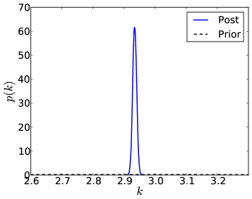
(a) $k$

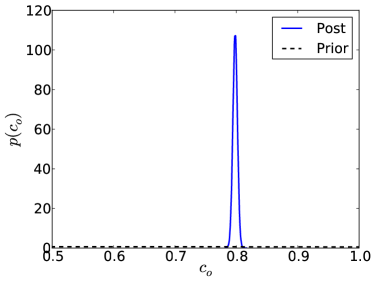
(b) $c$

Figure 1: Marginal distributions for parameters $k$ and $c$. Shown are the posterior PDF resulting from a Bayesian calibration using the $m=1$ data in Table 1 (solid), and the prior (dashed).

Clearly, the marginal posterior PDFs are very narrow, indicating that $k$ and $c$ are highly constrained by the data. The maximum a posteriori (MAP) value of $k$ is roughly $2.95$, which is close the true value of $3.0$. The MAP value of $c$ is approximately 0.8. There is no “true” value of $c$ since the true damping coefficient is changing in time. However, this value is within the range of true values observed for the actual system for $m=1$.

The first validation challenge is to simply compare the output of the calibrated model with the calibration data, as shown in Figure 2.

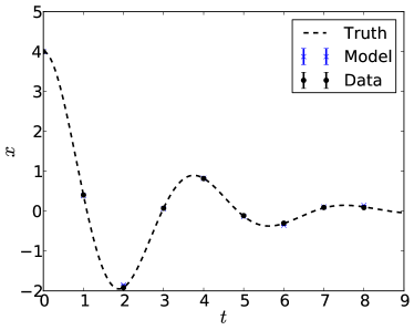
(a) All calibration data.

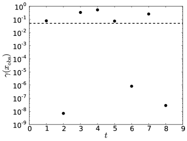
(b) HPRD credibility $\gamma$ at $x_{\mathrm{obs}}$ (21)

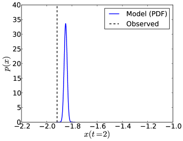
(c) $t=2.$

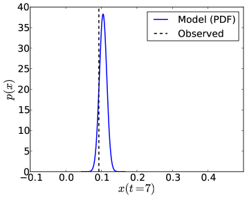
(d) $t=7.$

Figure 2: Comparison of output of calibrated model and observations for $m=1$ for SI0.

The figure shows the comparison in a number of different ways. Figure 2a shows the interval corresponding to the $5^{th}$ and $95^{th}$ percentiles according to both the model prediction and the observation plus its uncertainty. However, the errors are quite small relative to the largest values of $x$, making it difficult to assess the results. Figure 2b shows the HPRD credibility $\gamma$ (21), based on the distribution given by the model plus the observational uncertainty, and measured relative to a uniform distribution. To be clear, the model of the observation is given by

$$x_{\mathrm{obs}}=x_{m}+\epsilon,$$

where the distribution for $x_{m}$ is given by forward propagation of the joint posterior distribution for $k$ and $c$, and $\epsilon\sim N(0,0.01)$ is the observational noise. Figure 2b shows that for several of the observed data points, particularly those at $t=2$, $6$, and $8$, the corresponding $\gamma$ is less than or equal to approximately $10^{-6}$, indicating that the actual observation is far out on the tail of the prediction distribution. This can be clearly seen in Figure 2c, which shows the prediction distribution and the observation for $t=2$. Alternatively, for $t=7$, where $\gamma$ is significantly larger, there is much better agreement between the prediction distribution and the observation, as shown in Figure 2d.

However, the existence of points where the actual observation gives a $\gamma$ that is nearly zero shows that the model developed based on SI0 does not lead to plausible predictions even for the same data that was used to calibrate the model. In this situation, one must conclude that the uncertainty representation is unable to explain the differences between the physical model and the data. This fact contradicts the modeling assertion that the only important uncertainty is that due to measurement error. Since we cannot explain the observed discrepancies, we cannot confidently extrapolate to the prediction scenario using this model, even though the actual errors are not necessarily large. Despite the fact that the observed errors are not large, there is no way to characterize what the expected errors in the prediction scenario might be. Thus, the model is invalid for extrapolative prediction. Note that only the combination of the physical model and its uncertainty representation have been invalidated. It may be possible to improve either to obtain a model valid for use in the prediction. For example, we will see that the same physical model, when equipped with a better uncertainty description, can make valid predictions.

4.3.2 State of Information 1

SI1 does not provide enough information to allow extrapolation, regardless of the calibration and challenge results. Specifically, since we are completely ignorant of the mechanism causing the model inadequacy, we cannot form a plausible hypothesis that would enable extrapolation. This is a specific example of a general result, which is that without concrete hypotheses about the mechanisms causing the misfit between the model output and the data, extrapolation cannot be done with confidence. While the observed misfit can be modeled statistically, if the misfit cannot be explained, the effect of the observed errors cannot be extrapolated to the prediction. The situation is similar to SI0. We do not have a way to assess the effect of model inadequacy at the prediction scenario, and thus, cannot extrapolate with confidence.

4.3.3 State of Information 2

For SI2, at least there is enough information to form a hypothesis that, if correct, enables extrapolation to larger mass. Specifically, our hypothesis is that the range of variation of the damping coefficient $c$ decreases as mass increases. This hypothesis results from the observation that, in the system under study, the rate at which energy is dissipated by the damper is expected to decrease with increasing mass. For example, in the system under study, if the damping is weak, the average over an oscillation of the dissipation rate is given by $2ck/m$. Assuming that the temperature of the damping fluid is governed by a competition between how quickly energy is added to the fluid (by dissipation from the system) and how quickly energy is transferred to the surroundings, one would expect less temperature variation, and hence less variation in the damping coefficient, if energy is dissipated from the system more slowly. If this hypothesis is correct, a prediction made for a mass larger than that used to calibrate the model will be conservative—i.e., the predicted uncertainty should be larger than necessary to include the truth. Thus, the model can be valid in the sense of providing a conservative extrapolative prediction.

Of course, this is a qualitative argument, and any number of phenomena could be present in the real system that would make it invalid. Thus, we must assess this hypothesis—i.e., validate it—using observational data. After calibration, the validation and predictive assessment processes described below will focus on assessing this hypothesis.

Figure 3 shows the marginal PDFs resulting from the Bayesian calibration using the $m=1$ data.

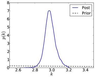
(a) $k$

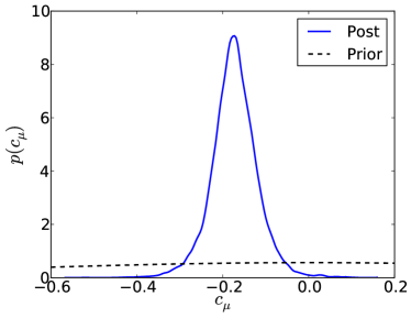
(b) $c_{\mu}$

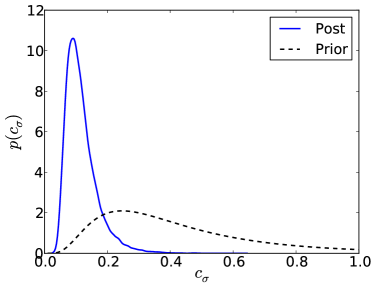
(c) $c_{\sigma}$

Figure 3: Marginal distributions for parameters $k$, $c_{\mu}$, and $c_{\sigma}$. The solid line labeled “Post” shows the marginal posterior PDF resulting from a Bayesian update of the prior (dashed line labeled “Prior”) using the $m=1$ data set (Table 1).

Note that the marginal posterior for $k$ is broader than in the SI0 result and that the (unknown) true value $k=3$ is in the support of the posterior PDF.

In the validation phase, the goal is to check that the model, is capable of representing both the $m=1$ data, on which it was calibrated, and the $m=2$ data. If any data point is highly unlikely according to the model, it is declared invalid, as happened with the SI0 model when it failed to reproduce the calibration data.

Figure 4 shows a comparison between the calibration data and the output of the calibrated model. The quantities shown in Figure 4 are analogous to those shown for SI0 in Figure 2, but unlike SI0, the predictions given are much more uncertain and agree better with the observations. In particular, the HPRD credibility, $\gamma$, shown in 4b are never less than approximately 0.4, indicating that the observations are near the highest probability density regions of the prediction distribution, as shown in Figures 4c and 4d.

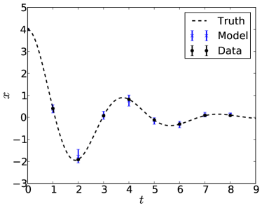
(a) All calibration data.

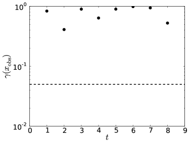
(b) HPRD credibility $\gamma$ at $x_{\mathrm{obs}}$ (21)

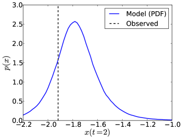
(c) $t=2.$

(d) $t=7.$

Figure 4: Comparison of output of calibrated model and observations for $m=1$ for SI2.

The same statement holds for the $m=2$ data, which was not used in calibration, as shown in Figure 5.

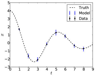
(a) All calibration data.

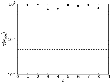
(b) HPRD credibility $\gamma$ at $x_{\mathrm{obs}}$ (21)

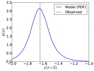
(c) $t=2.$

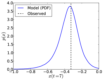
(d) $t=7.$

Figure 5: Comparison of output of calibrated model and observations for $m=2$ for SI2.

Since there is no evidence to invalidate the model after comparing the calibrated model predictions with all the available data, the validation phase is complete, and we may move on to the predictive assessment. To begin, recall that the predictive assessment is necessarily problem specific. In the current context, a reliable prediction is dependent on the hypothesis regarding the dependence of the variability of the damping coefficient on the mass. Thus, as part of predictive assessment, it is necessary to test this hypothesis to the fullest extent possible. Here, we test this hypothesis by performing a separate model calibration using the the $m=2$ data set. If the uncertainty in $c$ required to fit the $m=2$ data is smaller than that required to fit the $m=1$ data, as measured by the posterior results, then $c$ must be varied less to match the larger mass data, and the available data supports the hypothesis.

Figure 6 shows the results of this test.

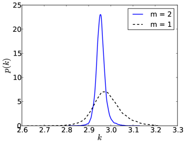
(a) $k_{s}$

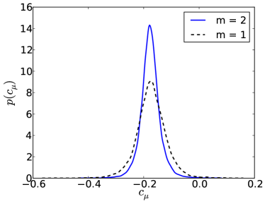
(b) $c_{\mu}$

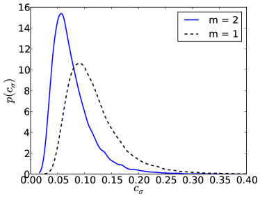
(c) $c_{\sigma}$

Figure 6: Comparison of marginal posterior PDFs obtained from a Bayesian update using the $m=2$ data (solid lines) versus the $m=1$ data (dashed lines).

The marginal posterior PDFs for $k$ and $c_{\mu}$ based on the two data sets are largely consistent, although the $m=2$ data somewhat better informs the parameters. However, $c_{\sigma}$, which is the standard deviation of $\log(c)$, moves significantly to the left. This result implies that the standard deviation of $c$ decreases. This fact is demonstrated in Figure 7, which shows the distribution of $c$ corresponding to the maximum likelihood values of $c_{\mu}$ and $c_{\sigma}$ as well as the PDF for the standard deviation of $c$ implied by the posterior joint distribution of $c_{\mu}$ and $c_{\sigma}$.

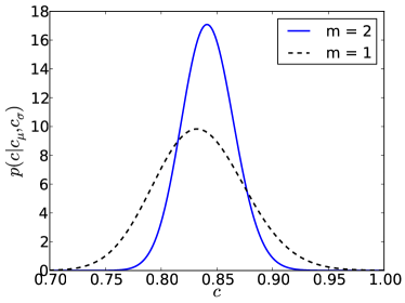
(a) Maximum likelihood result.

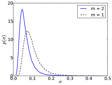
(b) Standard deviation of $c$.

Figure 7: Comparison of maximum likelihood log-normal distribution of $c$ and the PDF for the standard deviation of $c$ for the model calibrated using both the $m=1$ (dashed) and $m=2$ (solid) data.

Clearly the maximum likelihood distribution of $c$ is narrower when using the data from the larger mass. In particular, the standard deviation of the maximum likelihood model decreases from approximately $0.041$ to $0.023$, a decrease of nearly $44\%$. The distribution for $\sigma$ (the standard deviation of $c$) shows a similar result. When using the $m=2$ data, the probability distribution is shifted to lower values than when using the $m=1$ data, indicating that the variability of $c$ required to fit the data is decreasing with $m$. This result is consistent with the hypothesis.

Given this result, we can move to additional predictive assessments. In general, there may be many additional hypotheses to test or sensitivities to check, as discussed in §3.3. In this case we note that the data are quite informative about the parameters of the SI2 model (see Figure 3), indicating that there are no uninformed aspects of the model to which the predictions could be sensitive. Further, the “domain of applicability” of the model is implicitly checked (to the extent possible with the data) by the results of the calibration with the $m=2$ described previously. Thus, we conclude that there is good reason to trust the calibrated SI2 model to make credible predictions for the $m=5$ case.

Having challenged the model and the hypothesis needed to make extrapolation to larger masses possible, we are ready to make the prediction. Recall that the QoI is the maximum velocity for $m=5$. Figure 8 shows the prediction given by the model as well as the true value.

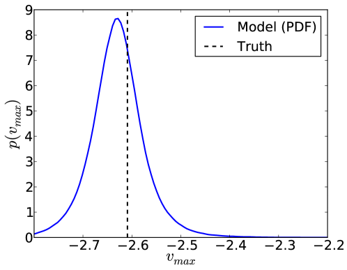
Figure 8: Prediction of maximum velocity for $m=5$.

Of course, in general the true value is unknown. It is given here just to show that the process has led us to the correct conclusion—i.e., the extrapolation is valid in the sense that the truth is assigned reasonable likelihood by the model.

Given this validated prediction, the next step would be to ask whether the predicted uncertainty is small enough to inform the desired decision. Since any tolerance we could specify here would be entirely contrived and artificial, we choose not to pursue this aspect. However, this is the simplest aspect of the predictive validation framework and should not cause significant difficulty. If the uncertainty is deemed too large, one would have to pose a better physical model, pose better uncertainty representations, get more data, or some combination of these, and begin the validation process again.

5 Conclusions

The predictive validation process proposed here provides a framework for building confidence in extrapolative predictions issued by models based on physics. There are two key ingredients enabling reliable extrapolation with such models. First, it is common that such models are based upon highly-reliable theory that is augmented with less-reliable embedded models to form a composite model. Second, the scenario dependence of the embedded models is generally different from the scenario of the full composite model, allowing the full model to be used for extrapolation without extrapolating the lower fidelity aspects. Given these ingredients, the predictive validation process requires the specification of a model inadequacy representation for the low-fidelity embedded models. This representation enables one to connect the QoI with observational data in a way that previous approaches lack. Once a physical model and inadequacy representation have been specified, the model is subjected to a calibration phase, where the observations are used to inform uncertain aspects of the model. Then, in validation, the model is challenged with new observational data. The primary question in this validation test is whether the observations are plausible given the uncertainty in the prediction. That is, the main objective of the validation is to test the combination of physical and uncertainty models. Finally, if the validation is satisfactory, the model is subjected to a predictive assessment to determine if the predictions of the QoIs can be trusted and whether they are sufficient from the point of view of a decision maker.

The full process has been illustrated using a simple spring-mass-damper system where the true physics of the damper are not well-understood by the modeler. Despite this lack of knowledge, the process is able to build confidence in a very simple model. However, this gain in confidence is contingent on the information available at the beginning of the process. With some specific knowledge regarding the cause of the modeling error, one may be able to build confidence in an inadequate model for making a particular prediction. Without this kind of information—i.e., simply knowing that the model does not match reality and nothing more—one will generally be able to do very little.

While the global process presented here is clear, there are several research and development issues that need to be addressed to enable the validation of such predictions in a wide range of applications. These research challenges are outlined briefly below.

1. Inadequacy models: A critical component of the proposed process is a probabilistic model of the errors in the embedded models. Such an inadequacy model should respect all that is known about the approximations and deficiencies of the models, all that is known about the quantities being modeled, and the available data. Broadly applicable techniques for formulating these inadequacy models are needed, especially for situations where the modeled quantity is a field.

2. Data uncertainty models: The uncertainty in experimental data is a critical input to the process, and better characterizations of this uncertainty are needed. Of particular concern are characterizing dependencies among different data points and uncertainties arising from data reduction modeling.

3. Representing qualitative information: In Bayesian analysis, posing priors that faithfully represent what is known about the problem at hand is important to making reliable inference. Once the prior knowledge is expressed mathematically, one often has rigorous tools, e.g., maximum entropy, to construct the needed prior distribution. But, this knowledge is commonly qualitative and difficult to express mathematically. Tools and techniques are needed to formulate the kinds of qualitative knowledge we commonly have regarding physical models based on reliable theory, as discussed here. Representations of qualitative information are also important in characterizing modeling inadequacy and data uncertainty.

4. Domains of applicability: It is critical to predictive validation to identify when an embedded model is being used under conditions for which it has not been calibrated and validated. For many models, an appropriate set of model-specific scenario parameters has not been defined. Determining such scenario parameters is part of physical modeling, and therefore dependent on the phenomena being modeled, and it is in general a significant challenge. However, generally applicable tools and techniques for developing and evaluating such parameterizations are needed.

5. Experimental design: Data is needed for calibration and validation, but it is critical to have data that adequately informs the QoIs in the context of the models. That is, measurements of quantities that are sensitive to the same uncertainties as the QoIs are needed under scenarios that will produce a sufficiently large domain of applicability for the embedded models. Metrics are needed to rank potential validation cases, allowing the best experimental measurements and scenarios to be determined automatically.

6. Computational algorithms: While we have not discussed the computational tools needed to execute the predictive validation process discussed here, there are significant algorithmic challenges associated with high dimensional probability spaces (the curse of dimensionality), with expensive computational models and with stochastic models, which arise naturally from the inadequacy representations discussed here.

As should be clear in the above discussion, research challenges 1-4 essentially require introducing knowledge about the physical phenomena being modeled into the process. Advancing techniques to address these challenges will presumably require pursuing them in the context of a variety of specific physical systems.

Appendix A Truth System

The truth system is similar to the physical model discussed in §4. However, instead of having a constant damping coefficient, the damping coefficient is a function of the temperature of the damper fluid. This situation is inspired by a fluid damper where the viscosity of the damper fluid, and hence the damping coefficient, varies with temperature. Here, the temperature of the fluid damper is determined by an ODE that includes the effect of energy dissipated by the damper and heat transferred from the damper to the surroundings, which are assumed to have constant temperature.

The equations are as follows:

$$m\ddot{x}+c(T)\dot{x}+kx=0$$

$$\dot{T}=c(T)\dot{x}^{2}-\frac{1}{\tau}\left(T-T_{0}\right)$$

where $k$, $T_{0}$, and $\tau$ are constants and

$$c(T)=\exp\left(\frac{T_{0}}{T}-1\right).$$

For all cases, the constants are set to the following values:

$$k=3,\quad T_{0}=20,\quad\tau=1.$$

References

- AIAA Computational Fluid Dynamics Committee on Standards [1998] AIAA Computational Fluid Dynamics Committee on Standards, 1998. AIAA Guide for Verification and Validation of Computational Fluid Dynamics Simulations. AIAA Paper number G-077-1999.
- Ainsworth and Oden [2000] Ainsworth, M., Oden, J., 2000. A posteriori error estimation in finite element analysis. John Wiley and Sons, Inc.
- ASME Committee V&V 10 [2006] ASME Committee V&V 10, 2006. Standard for Verification and Validation in Computational Solid Mechanics. ASME.
- ASME Committee V&V 20 [2009] ASME Committee V&V 20, 2009. Standard for Verification and Validation in Computational Fluid Dynamics and Heat Transfer. ASME.
- Babuška et al. [2007] Babuška, I., Nobile, F., Tempone, R., 2007. Reliability of computational science. Numerical Methods For Partial Differential Equations 23 (4), 753–784.
- Babuška et al. [2008] Babuška, I., Nobile, F., Tempone, R., 2008. A systematic approach to model validation based on Bayesian updates and prediction related rejection criteria. Computer Methods in Applied Mechanics and Engineering. 197, 2517–2539.
-
Balci [1997]
Balci, O., 1997. Verification validation and accreditation of simulation
models. In: Proceedings of the 29th Winter Simulation Conference. WSC ’97.
IEEE Computer Society, Washington, DC, USA, pp. 135–141.
URL http://dx.doi.org/10.1145/268437.268462 -
Bayarri et al. [2007]
Bayarri, M. J., Berger, J. O., Paulo, R., Sacks, J., Cafeo, J. A., Cavendish,
J., Lin, C.-H., Tu, J., 2007. A framework for validation of computer models.
Technometrics 49 (2), 138–154.
URL http://amstat.tandfonline.com/doi/abs/10.1198/004017007000000092 - Biegler et al. [2010] Biegler, L., Biros, G., Ghattas, O., Heinkenschloss, M., Keyes, D., Mallick, B., Marzouk, Y., Tenorio, L., van Bloemen Waanders, B., Willcox, K., 2010. Large-Scale Inverse Problems and Quantification of Uncertainty. John Wiley and Sons, Ltd, Chichester, UK.
- Box and Tiao [1973] Box, G., Tiao, G. C., 1973. Bayesian Inference in Statistical Analysis. New York: Wiley Classics.
- Cox [1961] Cox, R. T., 1961. The Algebra of Probable Inference. Johns Hopkins University Press, Baltimore, MD.
-
Craig et al. [2001]
Craig, P. S., Goldstein, M., Rougier, J. C., Seheult, A. H., 2001. Bayesian
forecasting for complex systems using computer simulators. Journal of the
American Statistical Association 96, 717–729.
URL http://EconPapers.repec.org/RePEc:bes:jnlasa:v:96:y:2001:m:june:p:717-729 -
Higdon et al. [2005]
Higdon, D., Kennedy, M., Cavendish, J. C., Cafeo, J. A., Ryne, R. D., Feb.
2005. Combining field data and computer simulations for calibration and
prediction. SIAM J. Sci. Comput. 26 (2), 448–466.
URL http://dx.doi.org/10.1137/S1064827503426693 - Hyndman [1996] Hyndman, R. J., 1996. Computing and graphing highest density regions. The American Statistician 50 (2), 120–126.
- Jaynes [2003] Jaynes, E. T., 2003. Probability Theory: The Logic of Science. Cambridge University Press.
-
Kennedy and O’Hagan [2001]
Kennedy, M. C., O’Hagan, A., 2001. Bayesian calibration of computer models.
Journal of the Royal Statistical Society: Series B (Statistical Methodology)
63 (3), 425–464.
URL http://dx.doi.org/10.1111/1467-9868.00294 -
Morrison et al. [2013]
Morrison, R. E., Bryant, C. M., Terejanu, G., Prudhomme, S., Miki, K., 2013.
Data partition methodology for validation of predictive models. Computers and
Mathematics with Applications 66 (10), 2114 – 2125.
URL http://dx.doi.org/10.1016/j.camwa.2013.09.006 - Oberkampf and Roy [2010] Oberkampf, W., Roy, C., 2010. Verification and Validation in Scientific Computing. Cambridge University Press.
- Oberkampf and Trucano [2007] Oberkampf, W. L., Trucano, T. G., 2007. Verification and Validation Benchmarks. Tech. Rep. SAND2007-0853, Sandia National Laboratories, Unlimited Release.
-
Oden et al. [2013]
Oden, J. T., Prudencio, E. E., Bauman, P. T., 2013. Virtual model validation of
complex multiscale systems: Applications to nonlinear elastostatics. Computer
Methods in Applied Mechanics and Engineering 266, 162 – 184.
URL http://dx.doi.org/10.1016/j.cma.2013.07.011 -
Panesi et al. [2012]
Panesi, M., Miki, K., Prudhomme, S., Brandis, A., 2012. On the assessment of a
bayesian validation methodology for data reduction models relevant to shock
tube experiments. Computer Methods in Applied Mechanics and Engineering
213–-216, 383–398.
URL http://dx.doi.org/10.1016/j.cma.2011.11.001 -
Prudhomme and Oden [1999]
Prudhomme, S., Oden, J., 1999. On goal-oriented error estimation for elliptic
problems: application to the control of pointwise errors. Computer Methods in
Applied Mechanics and Engineering 176 (1–4), 313 – 331.
URL http://dx.doi.org/10.1016/S0045-7825(98)00343-0 - Roache [2008] Roache, P. J., 2008. Perspective: Validation—What Does it Mean? ASME Journal of Fluids Engineering 131 (3), 1–3.
- Roache [2009] Roache, P. J., 2009. Fundamentals of Verification and Validation. Hermosa Publishers, Albuquerque.
-
Sargent [1998]
Sargent, R. G., 1998. Verification and validation of simulation models. In:
Proceedings of the 30th Winter Simulation Conference. WSC ’98. IEEE Computer
Society Press, Los Alamitos, CA, USA, pp. 121–130.
URL http://dl.acm.org/citation.cfm?id=293172.293216 - Strong et al. [2011] Strong, M., Oakley, J. E., Chilcott, J., 2011. Managing structural uncertainty in health economic decision models: a discrepancy approach. Journal of the Royal Statistical Society: Series C (Applied Statistics).
- Van Horn [2003] Van Horn, K. S., 2003. Constructing a logic of plausible inference: A guide to Cox’s theorem. International Journal of Approximate Reasoning 34 (1), 3–24.