Multiphase lattice Boltzmann simulations for porous media applications

Abstract

Over the last two decades, lattice Boltzmann methods have become an increasingly popular tool to compute the flow in complex geometries such as porous media. In addition to single phase simulations allowing, for example, a precise quantification of the permeability of a porous sample, a number of extensions to the lattice Boltzmann method are available which allow to study multiphase and multicomponent flows on a pore scale level. In this article we give an extensive overview on a number of these diffuse interface models and discuss their advantages and disadvantages. Furthermore, we shortly report on multiphase flows containing solid particles, as well as implementation details and optimization issues.

1 Introduction

Fluid flow in porous media is a topic which is relevant in the context of hydrocarbon production, groundwater flow, catalysis or the gas diffusion layers in fuel cells Hil96 . Oil and gas transport in porous rock PhysRevB.45.7115 , the flow in underground reservoirs and the propagation of chemical contaminants in the vadose zone 2005EG:DN ; citeulike:481254 , permeation of ink in paper koponen:3319 and filtration and sedimentation operations 2003IJMP:GCB are just a few examples from a wealth of possible applications. Most of these examples involve not only single phase flows, but multiple phases or fluid components. As such, a thorough understanding of the underlying physical processes by means of computer simulations requires accurate and reliable numerical tools.

Multiphase flows in porous media are typically modeled using macro-scale simulations, in which the continuity equation together with momentum and species balances are solved and constitutive equations such as Darcy’s law are utilized. These models are based on the validity of the constitutive relationships (e.g. the multiphase extension of Darcy’s Law), require some inputs for semi-empirical parameters (e.g. relative permeability), and have difficulties in accounting for heterogeneity, and complex pore interconnectivity and morphologies Balhoff2008 . As a result, macroscale simulations do not always capture effects associated with the microscale structure in multiphase flows. On the contrary, pore-scale simulations are able to capture heterogeneity, interconnectivity, and non-uniform flow behavior (e.g. various fingerings) that cannot be well resolved at the macroscopic scale. In addition, pore-scale simulations can provide detailed local information on fluid distribution and velocity, and enable the construction and testing of new models or constitutive equations for macroscopic scales.

Pore-network models Blunt1991 ; Bryant1992 ; Al-Gharbi2005 ; Valvatne2005 ; Piri2005 ; Blunt2013 ; Joekar:2008 ; Joekar:2010 ; Raoof:2010 are a viable tool for understanding multiphase flows at the pore scale, and they are computationally efficient. These models, however, are based upon simplified representations of the complex pore geometry Jiang:2007 , which restricts their predictive capability and accuracy.

Traditional CFD methods such as the volume-of-fluid (VOF) method Hirt1981 ; Rider1998 ; Gueyffier1999 ; Ferrari2013 and level set (LS) method Osher1988 ; Sussman1998 ; Osher2003 simulate multiphase flows by solving the macroscopic Navier-Stokes equations together with a proper technique to track/capture the phase interface. It is challenging to use VOF and LS methods for pore-scale simulations of multiphase flows in porous media because of the difficulties in modeling and tracking the dynamic phase interfaces. Also, they have difficulties incorporating fluid-solid interfacial effects (e.g. surface wettability) in complex pore structures, which are consequences of microscopic fluid-solid interactions.

Unlike traditional CFD methods, which are based on the solution of macroscopic variables such as velocity, pressure, and density, the lattice Boltzmann method (LBM) is a pseudo-molecular method that tracks the evolution of the particle distribution function of an assembly of molecules and is built upon microscopic models and mesoscopic kinetic equations bib:benzi-succi-vergassola ; bib:qian-dhumieres-lallemand ; bib:succi-01 . The macroscopic variables are obtained from moment integration of the particle distribution function. Even shortly after its introduction more than twenty years ago, the LBM became an attractive alternative to direct numerical solution of the Stokes equation for single-phase flows in porous media and complex geometries in general 1990PhFl.2.2085C ; bib:qian-dhumieres-lallemand ; bib:ferreol-rothman . In the LBM for multiphase flow simulations, the fluid-fluid interface is not a sharp material line, but a diffuse interface of finite width. The effective slip of the contact line is caused by the relative diffusion of the two fluid components in the vicinity of the contact line. Therefore, there are no singularities in the stress tensor in the lattice Boltzmann simulation of moving contact-line problems while the no-slip condition is satisfied Briant2004 ; Briant2004a ; Chen2000b ; Kang2002 ; Kang2004 ; Kang2005 . In addition, unlike traditional CFD methods, there is no need for complex interface tracking/capturing/resconstruction techniques in the diffuse interface methods. Rather, the formation, deformation, and transport of the interface emerge through the simulation results Chen1998 . Furthermore, in the LBM all computations involve only local variables enabling highly efficient parallel implementations based on simple domain decomposition bib:jens-harvey-chin-venturoli-coveney:2005 . With more powerful computers becoming available it was possible to perform detailed simulations of flow in artificially generated geometries koponen:3319 ; bib:jens-zauner-weeber-hilfer:2008 ; bib:jens-narvaez:2010 ; bib:jens-narvaez-zauner-raischel-hilfer:2010 , tomographic reconstructions of sandstone samples bib:ferreol-rothman ; Martys99largescale ; MAKHT02 ; bib:jens-venturoli-coveney:2004 ; Ahren06 , or fibrous sheets of paper koponen:716 .

The remainder of this article is organised as follows: after a more detailed introduction to the LBM in Sec. 2, we review a number of different diffuse interface multiphase and multicomponent models in Sec. 3. Sec. 3 also introduces how particle suspensions can be simulated using the LBM. Sec. 4 summarizes a few typical details to be taken care of when implementing a lattice Boltzmann code and Sec. 5 is comprised of a collection of possible applications of the several multiphase/multicomponent models available. Sec. 6 summarizes our findings and the advantages and limitations of the various methods.

2 The lattice Boltzmann method

The LBM can be seen as the successor of the lattice gas cellular automaton (LGCA) which was first proposed in 1986 by Frisch, Hasslacher, and Pomeau bib:fhp , as well as by Wolfram bib:wolfram . The LBM overcomes some limitations of the LGCA such as not being Galilei-invariant and numerical noise due to the Boolean nature of the algorithm. In contrast to the LGCA coarse graining of the molecular processes is not obtained by tracking individual discrete mesoscopic fluid packets anymore. Instead, in the LBM the dynamics of the single-particle distribution function $f(\vec{x},\vec{v},t)$ representing the probability to find a fluid particle with position $\vec{x}$ and velocity $\vec{v}$ at time $t$ is tracked mcnamara_use_1988 ; higuera_boltzmann_1989 ; benzi_lattice_1992 ; chen_recovery_1992 ; qian_lattice_1992 . Then, the density and velocity of the macroscopically observable fluid are given by $\rho(\vec{x},t)=\int f{\mathrm{d}}\vec{v}$ and $\vec{u}(\vec{x},t)=\int f\vec{v}{\mathrm{d}}\vec{v}$, respectively. In the non-interacting, long mean free path limit and with no externally applied forces, the evolution of this function is described by the Boltzmann equation,

$$\left(\partial_{t}+\vec{v}\cdot\vec{\nabla}\right)f=\Omega[f].$$ (1)

The left hand side describes changes in the distribution function due to free particle motion. The collision operator $\Omega$ on the right hand side describes changes due to pairwise collisions. In general, this is a complicated integral expression, but it is commonly simplified to the linear Bhatnagar-Gross-Krook, or BGK form bib:bgk ,

$$\Omega[f]\simeq-\frac{1}{\tau}\left[f-f^{\mathrm{(eq)}}\right].$$ (2)

This collision operator describes the relaxation towards a Maxwell-Boltzmann equilibrium distribution $f^{\mathrm{(eq)}}$ at a time scale set by the characteristic relaxation time $\tau$. The distributions governed by the Boltzmann-BGK equation conserve mass, momentum, and energy, and obey a non-equilibrium form of the second law of thermodynamics bib:liboff . Moreover, the Navier-Stokes equations for macroscopic fluid flow are obeyed in the limit of small Knudsen and Mach numbers (see below) bib:chapman-cowling ; bib:liboff .

By discretizing the single-particle distribution in time and space, the lattice Boltzmann formulation is obtained. Here, the positions $\vec{x}$ on which $f$ is defined are restricted to nodes of a lattice, and the velocities are restricted to a set $\vec{e}_{i},i=1,...,N$ joining these nodes. $N$ varies betweeen implementations and we refer to the article of Qian qian_lattice_1992 for an overview. We restrict ourselves to the popular D2Q9 and D3Q19 realizations, which correspond to a 2D lattice with 9 possible velocities and a 3D lattice with 19 possible velocities, respectively. To simplify the notation, $f_{i}(\vec{x},t)=f(\vec{x},\vec{e}_{i},t)$ represents the probability to find particles at a lattice site $\vec{x}$ moving with velocity $\vec{e}_{i}$, at the discrete timestep $t$. The density and momentum of the simulated fluid are calculated as

$$\rho(\vec{x},t)=\rho_{0}\sum_{i}f_{i}(\vec{x},t),$$ (3)

and

$$\rho(\vec{x},t)\vec{u}(\vec{x},t)=\sum_{i}f_{i}(\vec{x},t)\vec{e}_{i},$$ (4)

where $\rho_{0}$ refers to a reference density which is kept at $\rho_{0}=1$ in the remainder of this article. The pressure of the fluid is calculated via an isothermal equation of state,

$$\ p=c_{s}^{2}\rho.$$ (5)

Here, $c_{s}=c/\sqrt{3}$ is the lattice speed of sound and $c=\delta_{x}/\delta_{t}$ is the lattice speed. The lattice must be chosen carefully to ensure isotropic behavior of the simulated fluid bib:qian-dhumieres-lallemand . The lattice Boltzmann formulation can be obtained using alternative routes, including discretizing the continuum Boltzmann equation bib:he-luo , or regarding it as a Boltzmann-level approximation of the LGCA bib:mcnamara-zanetti .

The LBM follows a two-step procedure, namely an advection step followed by a collision step. In the advection step, values of the distribution function are propagated to adjacent lattice sites along their velocity vectors. This corresponds to the left-hand side of the continuum Boltzmann equation. In the collision step, particles at each lattice site are redistributed across the velocity vectors. This process corresponds to the action of the collision operator, and in the most simple case takes the BGK form. The combination of the advection and collision steps results in the lattice Boltzmann equation (LBE),

$$f_{i}(\vec{x}+\vec{e}_{i}\delta_{t},t+\delta_{t})-f_{i}(\vec{x},t)=\Omega_{i}(\vec{x},t).$$ (6)

In most applications and the remainder of this article the reference density, timestep and lattice constant are chosen to be $\rho_{0}=1$, $\delta_{t}=1$ and $\delta_{x}=1$. The discretized local equilibrium distribution is often given by a second order Taylor expansion of the Maxwell-Boltzmann equilibrium distribution,

$$f_{i}^{eq}=w_{i}\rho\left(1+\frac{1}{c_{s}^{2}}\vec{e}_{i}\cdot\vec{u}+\frac{1}{2c_{s}^{4}}(\vec{e}_{i}\cdot\vec{u})^{2}-\frac{1}{2c_{s}^{2}}|\vec{u}|^{2}\right).$$ (7)

Therein, the coefficients including the weights $w_{i}$ associated to the lattice discretisation and the speed of sound $c_{s}$ are determined by a comparison of a first order Chapman-Enskog expansion to the Navier-Stokes equations. The kinematic viscosity of the fluid,

$$\nu={c_{s}^{2}}\left(\tau-\frac{1}{2}\right),$$ (8)

is determined by the relaxation parameter $\tau$.

While the simplicity of the LBGK method has enabled it to be successfully applied to a wide range of problems chen_lattice_1998 ; bib:succi-01 ; aidun_lattice-boltzmann_2010 , it also implies limitations to the formalism. The implicit relationship between fluid properties and discretization parameters in Eq. 8 leads to numerical instability at lower viscosities lallemand_theory_2000 . As indicated by the equation of state in Eq. 5, the LBM approximates the Navier-Stokes equations in the near-incompressible limit. To minimise compressibility errors, and to adhere to the small-velocity assumption, the Mach number, $Ma=u/c_{s}$, has to be kept small (i.e. $Ma\ll 1$).

To address some of these limitations, different approaches and extensions to the formalism have been introduced. At an early stage of the LBM’s development, alternative collision schemes were introduced bib:higuera-succi-benzi ; dhumieres_generalized_1994 . In particular, the multiple relaxation time (MRT) collision operator can be written as ladd_numerical_1994 ; dhumieres_generalized_1994 ; dhumieres_multiplerelaxationtime_2002 ,

$$\Omega_{i}^{MRT}(\vec{x},t)=-\mathcal{M}^{-1}\mathcal{\hat{S}}\mathcal{M}\left[\ket{f(\vec{x},t)}-\ket{f^{eq}(\vec{x},t)}\right].$$ (9)

Herein $\mathcal{M}$ is an invertible transformation matrix, relating the moments of the single particle velocity distribution $f$ to linear combinations of its discrete components $f_{i}$. It can be obtained by a Gram Schmidt orthogonalization of a matrix representation of the stochastical moments. The collision process is performed in the space of moments, where $\mathcal{\hat{S}}$ is a diagonal matrix of the individual relaxation times. Thus, independent transport coefficients are introduced. For example, in addition to the shear viscosity, the bulk viscosity $\xi=c_{s}^{2}\left({\tau_{\mathsf{bulk}}}-\frac{1}{2}\right)$ can be controlled dhumieres_multiplerelaxationtime_2002 .

Starting from this general approach, simplifications and extensions have led to the development of, for example, two relaxation time (TRT) models ginzburg_equilibrium-type_2005 ; ginzburg_optimal_2010 as well as models incorporating thermal fluctuations ladd_short-time_1993 ; dunweg_statistical_2007 ; gross_thermal_2010 ; kaehler_fluctuating_2013 .

Further refinement of the method has been achieved by identifying general formalisms for deriving higher order expansions of the equilibrium distribution and lattice discretisations allowing to include higher order effects into the model shan_kinetic_2006 ; dubois_towards_2009 .

The ease in handling boundaries is one of the reasons for the LBM being well suited to simulating porous media flows. Many boundary condition implementations maintain the locality of LBE operations, which means that tortuous pore network geometries can be modeled on an underlying orthogonal grid, and that parallelization of the method remains straightforward.

The simplest approach to model the interaction of fluid and solid is the bounce-back scheme. It enforces the no-slip condition at solid surfaces by reflecting particle distribution functions from the boundary nodes back in the direction of incidence. Advantages of the bounce-back condition are that the required operations are local to a node and that the orientation of the boundary with respect to the grid is irrelevant. However, the simplicity of the bounce-back scheme is at the expense of accuracy. It has been shown that generally it is only first-order in numerical accuracy Cornubert1991 as opposed to the second order accuracy of the lattice Boltzmann equation at internal fluid nodes bib:chen-doolen . It has also been shown bib:pf.QZoXHe.1997 that the bounce-back condition actually results in a boundary with a finite relaxation time dependent slip narvaez_quantitative_2010 . Nevertheless, the bounce-back scheme is usually suitable for simulating the fluid interaction at stationary boundaries such as the Dolomite rock sample shown in Fig. 1.

Pressure and velocity boundary conditions can be applied in the LBM by assigning particle distribution functions at a node which correspond to the prescribed macroscopic constraint. As an example, Zou and He bib:pf.QZoXHe.1997 proposed a boundary condition based on bouncing-back the non-equilibrium part of the distribution function. It can be applied to velocity, pressure and wall constraints. As with the bounce-back condition, all required operations are local. While the original implementation was limited to two dimensions and boundaries parallel to the orthogonal lattice directions, Hecht and Harting presented how to overcome these limitations HH08b . Periodic and stress-free boundary implementations are also available, and a detailed review of other velocity boundary condition implementations in the LBM can be found in Latt2008 .

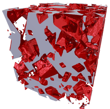
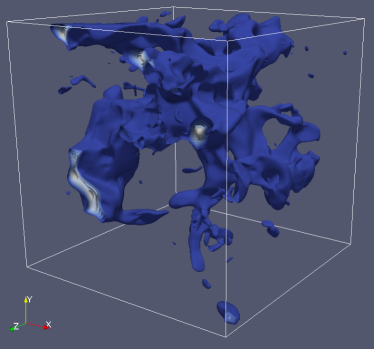
Figure 1: Single phase flow in a segmented, $\mu$CT image of a Dolomite sample including 1 a rendering of the pore volume (i.e. the complement of the rock volume) in the sample and 2 the steady state flow profile in the sample as computed by the LBM with bounce-back boundary conditions.

3 Review of Multiphase$/$Multicomponent LBM Formulations

A number of multiphase LBM models have been proposed in the literature. Among them, five representative models are the color gradient model Gunstensen1991 ; Reis2007 ; Liu2012a , the inter-particle potential model Shan1993 ; Shan1994 ; Shan1995 , the free-energy model Swift1995 ; Swift1996 , the mean-field theory model He1999 , and the stabilized diffuse-interface model Lee2010 . In this section, we review these models with emphasis on some recent improvements and show their advantages and limitations for pore-sale simulation of multiphase flows in porous media.

3.1 The color gradient model

The color gradient model originated from the two-component lattice-gas model proposed by Rothman & Keller Rothman1988 , and was first introduced by Gunstensen et al. Gunstensen1991 for simulating immiscible binary fluids based on a two-dimensional(2D) hexagonal lattice. Later, it was modified by Grunau et al. Grunau1993 to allow variations of density and viscosity. In this model, “Red” and “Blue” distribution functions $f_{i}^{R}$ and $f_{i}^{B}$ were introduced to represent two different fluids. The total particle distribution function is defined as: $f_{i}=f_{i}^{R}+f_{i}^{B}$. Each of the colored fluids undergoes the collision and streaming steps,

$$f_{i}^{k{\dagger}}(\vec{x},t)=f_{i}^{k}(\vec{x},t)+\Omega_{i}^{k}(\vec{x},t),$$ (10)

$$f_{i}^{k}(\vec{x}+\vec{e}_{i}\delta_{t},t+\delta_{t})=f_{i}^{k{\dagger}}(\vec{x},t),$$ (11)

where the superscript $k=R$ or $B$ denotes the color (“Red” or “Blue”), and the collision operator $\Omega_{i}^{k}$ consists of three sub-operators Tolke2002a ; Liu2012a ,

$$\Omega_{i}^{k}=(\Omega_{i}^{k})^{(3)}\left[(\Omega_{i}^{k})^{(1)}+(\Omega_{i}^{k})^{(2)}\right].$$ (12)

In Eq.(12), $(\Omega_{i}^{k})^{(1)}$ is the BGK collision operator, defined as $(\Omega_{i}^{k})^{(1)}=-\frac{1}{\tau_{k}}(f_{i}^{k}-f_{i}^{k,eq})$, where $\tau_{k}$ is the dimensionless relaxation time of fluid $k$, and $f_{i}^{k,eq}$ is the equilibrium distribution function of $f_{i}^{k}$. Conservation of mass for each fluid and total momentum conservation require,

$$\rho_{k}=\sum_{i}f_{i}^{k}=\sum_{i}f_{i}^{k,eq},$$ (13)

$$\rho\vec{u}=\sum_{i}\sum_{k}f_{i}^{k}\vec{e}_{i}=\sum_{i}\sum_{k}f_{i}^{k,eq}\vec{e}_{i},$$ (14)

where $\rho_{k}$ is the density of fluid $k$, $\rho=\rho_{R}+\rho_{B}$ is the total density and $\vec{u}$ the local fluid velocity.

$(\Omega_{i}^{k})^{(2)}$ is a two-phase collision operator (i.e. perturbation step) which contributes to the mixed interfacial region and generates an interfacial tension. For a 2D hexagonal lattice, the perturbation operator is given as Gunstensen1991 ; Grunau1993 ,

$$(\Omega_{i}^{k})^{(2)}=\frac{A_{k}}{2}|\vec{G}|\left[\frac{(\vec{e}_{i}\cdot\vec{G})^{2}}{|\vec{G}|^{2}}-\frac{1}{2}\right],$$ (15)

where $A_{k}$ is a free parameter controlling the interfacial tension, and $\vec{G}$ is the local color gradient which is defined by $\vec{G}(\vec{x},t)=\sum_{i}[\rho_{R}(\vec{x}+\vec{e}_{i},t)-\rho_{B}(\vec{x}+\vec{e}_{i},t)]\vec{e}_{i}$. However, Reis & Phillips Reis2007 and Liu et al. Liu2012a found that, a direct extension of the perturbation operator Eq. (15) to popular D2Q9 and D3Q19 lattices cannot recover the correct Navier-Stokes equations for two-phase flows. To obtain the correct interfacial force term for the D2Q9 lattice, Reis & Phillips proposed an improved perturbation operator Reis2007 ,

$$(\Omega_{i}^{k})^{(2)}=\frac{A_{k}}{2}|\vec{G}|\left[w_{i}\frac{(\vec{e}_{i}\cdot\vec{G})^{2}}{|\vec{G}|^{2}}-B_{i}\right],$$ (16)

where $w_{i}$ is the weight factor, and $B_{0}=-\frac{4}{27}$, $B_{1-4}=\frac{2}{27}$ and $B_{5-8}=\frac{5}{108}$. Using the concept of a continuum surface force (CSF) together with the constraints of mass and momentum conservation, a generalized perturbation operator was derived recently by Liu et al. Liu2012a for the D3Q19 lattice,

$$(\Omega_{i}^{k})^{(2)}=\frac{A_{k}}{2}|\nabla\rho^{N}|\left[w_{i}\frac{(\vec{e}_{i}\cdot\nabla\rho^{N})^{2}}{|\nabla\rho^{N}|^{2}}-B_{i}\right],$$ (17)

where the phase field $\rho^{N}$ is defined as

$$\rho^{N}(\vec{x},t)=\frac{\rho_{R}(\vec{x},t)-\rho_{B}(\vec{x},t)}{\rho_{R}(\vec{x},t)+\rho_{B}(\vec{x},t)},\quad-1\leq\rho^{N}\leq 1,$$ (18)

and

$$B_{0}=-\frac{2+2\chi}{3\chi+12}c^{2},\quad B_{1-6}=\frac{\chi}{6\chi+24}c^{2},\quad B_{7-18}=\frac{1}{6\chi+24}c^{2},$$ (19)

with $\chi$ being a free parameter. In addition, an expression for interfacial tension $\sigma$ was analytically obtained without any additional analysis and assumptions Liu2012a ,

$$\sigma=\frac{2}{9}(A_{R}+A_{B})\tau,$$ (20)

where $\tau$ is the relaxation time of the fluid mixture. Its validity was demonstrated by stationary bubble tests Liu2012a . Eq. (20) suggests that the interfacial tension can be flexibly chosen by controlling $A_{R}$ and $A_{B}$.

To promote phase segregation and maintain the interface, the recoloring operator $(\Omega_{i}^{k})^{(3)}$ is applied, which enables the interface to be sharp, and at the same time prevents the two fluids from mixing with each other. There are two recoloring algorithms widely used in the literature, namely the recoloring algorithm of Gunstensen et al. Gunstensen1991 and the recoloring algorithm of Latva-Kokko and Rothman Latva-Kokko2005 , which are hereafter referred to as A1 and A2, respectively. In A1, the distribution functions $f_{i}^{R{\dagger}}(\vec{x},t)$ and $f_{i}^{B{\dagger}}(\vec{x},t)$ are found by maximizing the work done by the color gradient,

$$\sum_{i}[f_{i}^{R{\dagger}}(\vec{x},t)-f_{i}^{B{\dagger}}(\vec{x},t)]\vec{e}_{i}\cdot\vec{G},$$ (21)

subject to the constraints of local conservation of the individual fluid densities of the two components, and local conservation of the total distribution function in each direction. This recoloring algorithm can produce a very thin interface, but generates velocity fluctuations even for a non-inclined planar interface Tolke2002a . In addition, when applied to creeping flows, this recoloring algorithm can produce lattice pinning, a phenomenon where the interface can be pinned or attached to the simulation lattice rendering an effective loss of Galilean invariance Latva-Kokko2005 . It was also identified that there is an increasing tendency for lattice pinning as both the Capillary and Reynolds numbers decrease Halliday2006 . Therefore, this algorithm is not effective for simulating multiphase flows in porous media, especially when the capillary force is dominant. In A2, the recoloring operator is defined as Liu2012a ,

$$(\Omega_{i}^{R})^{(3)}(f_{i}^{R})=\frac{\rho_{R}}{\rho}f_{i}^{*}+\beta\frac{\rho_{R}\rho_{B}}{\rho^{2}}\cos(\varphi_{i})f_{i}^{eq}|_{\vec{u}=0},$$ (22)

$$(\Omega_{i}^{B})^{(3)}(f_{i}^{B})=\frac{\rho_{B}}{\rho}f_{i}^{*}-\beta\frac{\rho_{R}\rho_{B}}{\rho^{2}}\cos(\varphi_{i})f_{i}^{eq}|_{\vec{u}=0},$$ (23)

where $f_{i}^{*}$ denotes the post-perturbation, pre-segregation value of the total distribution function along the $i$-th lattice direction, and $f_{i}^{eq}=\sum_{k}f_{i}^{k,eq}$ is the total equilibrium distribution function. $\beta$ is the segregation parameter related to the interface thickness, and its value must be between 0 and 1 to ensure positive particle distribution functions. $\varphi$ is the angle between the color gradient $\vec{G}$ and the lattice vector $\vec{e}_{i}$, which is defined by,

$$\cos(\varphi_{i})=\frac{\vec{e}_{i}\cdot\nabla\vec{G}}{|\vec{e}_{i}||\nabla\vec{G}|}.$$ (24)

Note that $\vec{G}$ should be replaced by the phase field gradient $\nabla\rho^{N}$ when the perturbation operator Eq. (17) is applied. Leclaire et al. Leclaire2012 conducted a numerical comparison of the recoloring operators A1 and A2 for an immiscible two-phase flow by a series of benchmark cases and concluded that the recoloring operator A2 greatly increases the rate of convergence, improves the numerical stability and accuracy of the solutions over a broad range of model parameters, and significantly reduces spurious velocities and relieves the lattice pinning problem. Several recent numerical studies Leclaire2011 ; Liu2012a indicated that, for a combination of Eq. (17) and the recoloring algorithm A2, the simulated density ratio and viscosity ratio can be up to $O(10^{3})$ for stationary bubble/droplet tests, whereas for dynamic problems the simulated density ratio is restricted to $O(10)$ due to numerical instability.

3.2 Inter-particle potential model

Shan and Chen Shan1993 developed an inter-particle potential model (also known as Shan-Chen model) through introducing microscopic interactions among nearest-neighboring particles. The mean field force is incorporated by using a modified equilibrium velocity in the collision operator. This force ensures phase separation and introduces interfacial tension. The inter-particle potential model includes two types, namely the single-component multiphase (SCMP) model Shan1993 ; Shan1994 and the multicomponent multiphase (MCMP) model Shan1993 ; Shan1995 . In this section, we only introduce the MCMP inter-particle potential model in the model description for the sake of conciseness, while the capability of SCMP model and several relevant studies are still reviewed.

The LBE for the $k$th fluid is given by,

$$f_{i}^{k}(\vec{x}+\vec{e}_{i}\delta_{t},t+\delta_{t})=f_{i}^{k}(\vec{x},t)-\frac{1}{\tau_{k}}\left[f_{i}^{k}(\vec{x},t)-f_{i}^{k,eq}(\vec{x},t)\right],$$ (25)

where the equilibrium distribution function $f_{i}^{k,eq}$ is written as,

$$f_{i}^{k,eq}=\rho_{k}w_{i}\left[1+\frac{3}{c^{2}}\vec{e}_{i}\cdot\vec{u}_{k}^{eq}+\frac{9}{2c^{4}}(\vec{e}_{i}\cdot\vec{u}_{k}^{eq})^{2}-\frac{3}{2c^{2}}|\vec{u}_{k}^{eq}|^{2}\right].$$ (26)

The macroscopic density and momentum of the $k$th fluid are defined by $\rho_{k}=\sum_{i}f_{i}^{k}$ and $\rho_{k}\vec{u}_{k}=\sum_{i}f_{i}^{k}\vec{e}_{i}$. The equilibrium velocity of the $k$th fluid is modified to carry the effect of the interactive force Shan1995 ; huang:066701 ,

$$\vec{u}_{k}^{eq}=\vec{u}^{\prime}+\frac{\tau_{k}\vec{F}_{k}}{\rho_{k}},$$ (27)

where $\vec{u}^{\prime}$ is a common velocity, which is taken as $\vec{u}^{\prime}=(\sum_{k}\frac{\rho_{k}\vec{u}_{k}}{\tau_{k}})/(\sum_{k}\frac{\rho_{k}}{\tau_{k}})$ to conserve the momentum in the absence of forces. $\vec{F}_{k}$ is the net force exerted on the $k$th fluid which includes both the fluid-fluid cohesion ($\vec{F}_{k}^{f-f}$) and the fluid-solid adhesion $\vec{F}_{k}^{f-s}$, so that $\vec{F}_{k}=\vec{F}_{k}^{f-f}+\vec{F}_{k}^{f-s}$.

In the inter-particle potential model, nearest neighbor interactions are used to model the fluid-fluid cohesive force Shan1995 ; huang:066701 ,

$$\vec{F}_{k}^{f-f}(\vec{x},t)=-G_{c}\psi_{k}(\vec{x},t)\sum_{i}w_{i}\psi_{\bar{k}}(\vec{x}+\vec{e}_{i}\delta_{t},t)\vec{e}_{i},$$ (28)

where is $G_{c}$ a parameter that controls the strength of the cohesive force, $k$ and $\bar{k}$ denote two different fluid components, and $\psi_{k}$ is the interaction potential (or “effective mass”) which is a function of local density. Analysis has shown that the interaction potential function has to be monotonically increasing and bounded Shan1993 . Several forms of the interaction potential are commonly utilized in the literature and include, for example $\psi_{k}=\rho_{k}$ Martys1996 ; huang:066701 and $\psi_{k}=1-\mathrm{e}^{-\rho_{k}}$ Shan1993 ; Schmieschek2011 . The force $\vec{F}_{k}^{f-f}$ allows the generation of interface between the different fluids and the equation of state is given by $p=\frac{1}{3}c_{s}^{2}\sum_{k}\rho_{k}+\frac{1}{6}G_{c}\sum_{k\bar{k}}\psi_{k}\psi_{\bar{k}}$ huang:066701 , where the first term corresponds to the ideal gas and the second term is the non-ideal part.

Repulsive interactions between two components ($G_{c}>0$) are utilised to model systems of partly miscible or immiscible fluid mixtures. While the input parameters are determined strictly phenomenologically, this approach has recently been shown equivalent to the explicit adjustment of the free energy of the system PhysRevE.84.036703 .

In the context of multiphase flow in oil reservoirs, surfactants are employed in enhanced oil recovery processes to alter the relative wettability of oil and water. Amphiphiles (i.e. surfactants) are comprised of a hydrophilic head group and a hydrophobic tail. Amphiphilic behaviour is modeled by a dipolar moment $\mathbf{d}$ with orientation $\theta$ defined for each lattice site. The relaxation is a BGK-like process, where the equilibrium moment is dependent on the surrounding fluid densities bib:nekovee-coveney-chen-boghosian . The introduction of the dipole vector accounts for three additional Shan-Chen type interactions, namely an additional force term,

$$\mathbf{F}^{k,s}=-2\psi^{k}(\mathbf{x},t)G_{k,s}\sum_{i\neq 0}\mathbf{\tilde{d}}(\mathbf{x}+\mathbf{e}_{i}\delta_{t},t)\cdot\mathbf{\Theta}_{i}\psi^{s}(\mathbf{x}+\mathbf{e}_{i}\delta_{t},t),$$ (29)

for the regular fluid components $k$ imposed by the surfactant species s. Therein, the tilde denotes post-collision values and the second rank tensor $\mathbf{\Theta}_{i}\equiv\mathbb{I}-3\frac{\mathbf{e}_{i}\mathbf{e}_{i}}{\delta_{x}^{2}}$, with the identity operator $\mathbb{I}$ weights the dipole force contribution according to the orientation relative to the density gradient. The surfactant species is subject to forcing as well, where the contribution of the regular components $k$ is given by,

$$\mathbf{F}^{k,s}=2\psi^{s}(\mathbf{x},t)\mathbf{\tilde{d}}(\mathbf{x},t)\cdot\sum_{k}G_{k,s}\sum_{i\neq 0}\mathbf{\Theta}_{i}\psi^{k}(\mathbf{x}+\mathbf{e}_{i}\delta_{t},t),$$ (30)

and,

$$\mathbf{F}^{ss}= -\frac{12}{\parallel\mathbf{c}_{s}\parallel^{2}}\psi^{s}(\mathbf{x},t)G_{s,s}\cdot\sum_{i\neq 0}\psi^{s}(\mathbf{x}+\mathbf{e}_{i}\delta_{t},t)\cdot\bigg{(}\mathbf{\tilde{d}}(\mathbf{x}+\mathbf{e}_{i}\delta_{t},t)\cdot\mathbf{\Theta}_{i}$$

$$\cdot\mathbf{\tilde{d}}(\mathbf{x},t)\mathbf{e}_{i}+\left[\mathbf{\tilde{d}}(\mathbf{x}+\mathbf{e}_{i}\delta_{t})\mathbf{\tilde{d}}(\mathbf{x},t)+\mathbf{\tilde{d}}(\mathbf{x},t)\mathbf{\tilde{d}}(\mathbf{x}+\mathbf{e}_{i}\delta_{t},t)\right]\cdot\mathbf{e}_{i}\bigg{)},$$

is the force due to self-interaction of the amphiphilic species bib:nekovee-coveney-chen-boghosian . The amphiphilic lattice Boltzmann model has been used successfully to describe domain growth in mixtures of simple liquids and surfactants bib:gonzalez-nekovee-coveney ; bib:emerton-coveney-boghosian ; bib:gonzalez-coveney-2 , the formation of mesophases such as the so-called primitive, diamond, and gyroid phases bib:jens-gonzalez-giupponi-coveney:2005 ; bib:jens-giupponi-coveney:2006 ; bib:jens-harvey-chin-venturoli-coveney:2005 ; bib:saksena-coveney-2009 , and to investigate the behaviour of amphiphilic mixtures in complex geometries such as microchannels and porous media bib:jens-kunert:2008b ; bib:jens-kunert-jari:2010 ; SNH12b .

Furthermore, a force exerted by a surface interaction can be introduced as bib:jens-kunert-herrmann:2006 ; Martys1996 ; huang:066701 ,

$$\vec{F}_{k}^{f-s}(\vec{x},t)=-G_{ads,k}\psi_{k}(\vec{x},t)\sum_{i}w_{i}s(\vec{x}+\vec{e}_{i}\delta_{t})\vec{e}_{i},$$ (32)

where $G_{ads,k}$ represents the strength of interaction between the fluid $k$ and the solid, and $s(\vec{x}+\vec{e}_{i}\delta_{t})$ is an indicator function which is equal to 1 for a solid node or 0 for a fluid node, respectively. When $\psi_{k}$ is chosen as $\rho_{k}$, Huang et al. huang:066701 proposed the following estimate for the contact angle $\theta$ (which is measured in fluid 1),

$$\cos(\theta)=\frac{G_{ads,2}-G_{ads,1}}{G_{c}\frac{\rho_{1}-\rho_{2}}{2}},$$ (33)

which suggests that different contact angles can be achieved by adjusting the parameters $G_{ads,k}$.

Recently, several methods have been developed to alleviate the limitations of the original inter-particle potential model and improve its performance. These techniques include incorporating a realistic equation of state into the model Yuan2006 ; Zhang2008 , increasing the isotropy order of the interactive force Shan2006 ; Sbragaglia2007 , improving the force scheme Kupershtokh2009 ; Huang2011 ; Li2012a ; Sun2012 , and using the Multi-Relaxation Time (MRT) scheme Yu2010 ; SNH12b instead of the BGK approximation. These techniques have been demonstrated to be effective in reducing the magnitude of spurious velocities, eliminating the unphysical dependence of equilibrium density and interfacial tension on viscosity (relaxation time), and increasing the viscosity and denstiy ratios in simple systems Porter2012 ; Bao2013 ; Yu2009 ; Kamali2012 ; Kamali2013 . As shown by Porter et al. Porter2012 , the 4th-order isotropy in the interactive force results in stable bubble simulations for a viscosity ratio of up to 300, whereas the 10th-order isotropy resultis in stable bubble simulations for a viscosity ratio of up to 1050. However, the effectiveness of these improved models in dealing with multiphase flow in complex porous media has not been fully investigated and is an active research topic. In a recent study it was found that the interfacial width associated with the interparticle potential model is significantly larger than for the colour gradient model or the free-energy model introduced below Yang:2013 . However, this finding could not be confirmed by the authors of the current paper. We find an interfacial width which is comparable to the free-energy model (about five lattice units).

3.3 Free-energy model

The free-energy model proposed by Swift et al. Swift1995 ; Swift1996 is built upon the phase-field theory, in which a free-energy functional is used to account for the interfacial tension effects and describe the evolution of interface dynamics in a thermodynamically consistent manner. Similar to the inter-particle potential model Shan1993 , the free-energy model also includes both SCMP model and MCMP models Swift1996 . The SCMP free-energy model can satisfy the local conservation of mass and momentum, but it suffers from a lack of Galilean invariance since density (pressure) gradients are of order $O(1)$ at liquid-gas interfaces. However, errors due to violation of Galilean invariance are insignificant for the MCMP free-energy model, which uses binary fluids with similar density so that the pressure gradients in the interfacial regions are much smaller Sman2008 . Therefore, the MCMP free-energy model has been applied to understand multiphase flows in porous media especially in the situation where inertial effects can be neglected Hao2010 ; Niu2007 .

In the MCMP free-energy model for two-phase system such as fluids ‘1’ and ‘2’ which have density of $\rho_{1}$ and $\rho_{2}$, respectively, two distribution functions $f_{i}(\vec{x},t)$ and $g_{i}(\vec{x},t)$ are used to model density $\rho=\rho_{1}+\rho_{2}$, velocity $\vec{u}$ and the order parameter $\phi$ which represents the different phases, respectively. The time evolution equations for the distribution functions, using the standard BGK approximation, can be written as,

$$f_{i}(\vec{x}+\vec{e}_{i}\delta_{t},t+\delta_{t})-f_{i}(\vec{x},t) = \frac{1}{\tau_{f}}[f_{i}^{eq}(\vec{x},t)-f_{i}(\vec{x},t)],$$ (34)

$$g_{i}(\vec{x}+\vec{e}_{i}\delta_{t},t+\delta_{t})-g_{i}(\vec{x},t) = \frac{1}{\tau_{g}}[g_{i}^{eq}(\vec{x},t)-g_{i}(\vec{x},t)],$$ (35)

where $\tau_{f}$ and $\tau_{g}$ are two independent relaxation parameters; $f_{i}^{eq}$ and $g_{i}^{eq}$ are the equilibrium distributions of $f_{i}$ and $g_{i}$.

The underlying physical properties of lattice Boltzmann schemes are determined via the hydrodynamic moments of the equilibrium distribution functions. The moments of the distribution functions should satisfy Swift1996

$$\sum_{i}f_{i}=\sum_{i}f_{i}^{eq}=\rho;\quad\sum_{i}g_{i}=\sum_{i}g_{i}^{eq}=\phi,$$ (36)

$$\sum_{i}f_{i}\vec{e}_{i}=\sum_{i}f_{i}^{eq}\vec{e}_{i}=\rho\vec{u};\quad\sum_{i}g_{i}^{eq}\vec{e}_{i}=\phi\vec{u},$$ (37)

$$\sum_{i}f_{i}\vec{e}_{i}\vec{e}_{i}^{T}=\vec{P}+\rho\vec{u}\vec{u}^{T};\quad\sum_{i}g_{i}\vec{e}_{i}\vec{e}_{i}^{T}=\Gamma\mu\vec{I}+\phi\vec{u}\vec{u}^{T},$$ (38)

where $\vec{P}$ is the pressure tensor, and $\Gamma$ is a coefficient which controls the phase interface diffusion and is related to the mobility $M$ of the fluid as follows Swift1996 ; Liu2009a ,

$$M=\Gamma\left(\tau_{g}-\frac{1}{2}\right)\delta_{t}.$$ (39)

Following the constraints of Eqs. (36)-(38), the equilibrium distributions $f_{i}^{eq}$ and $g_{i}^{eq}$, which are assumed to be a power series in terms of the local velocity, can be written as Liu2010 ,

$$f_{i}^{eq}=F_{i}+\rho w_{i}\left(\frac{3}{c^{2}}\vec{e}_{i}\cdot\vec{u}+\frac{9}{2c^{4}}(\vec{e}_{i}\cdot\vec{u})^{2}-\frac{3}{2c^{2}}|\vec{u}|^{2}\right),$$ (40)

$$g_{i}^{eq}=w_{i}\left[\frac{\Gamma\mu}{c_{s}^{2}}+\phi\left(\frac{3}{c^{2}}\vec{e}_{i}\cdot\vec{u}+\frac{9}{2c^{4}}(\vec{e}_{i}\cdot\vec{u})^{2}-\frac{3}{2c^{2}}|\vec{u}|^{2}\right)\right],$$ (41)

for a D2Q9 lattice with $i=1,...,8$, where the coefficient $F_{i}$ is given by,

$$F_{i}=\left\{\begin{array}[]{ll}\vec{e}_{i}^{T}\vec{P}\,\vec{e}_{i}/2c^{4}-(P_{xx}+P_{yy})/12c^{2}&\mbox{$i=1-4$},\\ \vec{e}_{i}^{T}\vec{P}\,\vec{e}_{i}/8c^{4}-(P_{xx}+P_{yy})/6c^{2}&\mbox{$i=5-8$}.\end{array}\right.$$ (42)

In addition, the equilibrium distributions for the rest particles are chosen to ensure mass conservation, $f_{0}^{eq}=\rho-\sum_{i>0}f_{i}^{eq}$ and $g_{0}^{eq}=\phi-\sum_{i>0}g_{i}^{eq}$.

The pressure tensor $\vec{P}$ and the interfacial tension in a two-phase system, as well as the wetting boundary condition at solid walls can be derived from the free-energy functional of the system, which is defined as a function of the order parameter $\phi$ as follows Briant2004a ,

$$\mathscr{F}(\phi)=\int_{V}\left(\Psi(\phi)+\frac{\kappa}{2}|\nabla\phi|^{2}+\rho c_{s}^{2}\ln\rho\right)dV+\int_{S}f_{w}(\phi_{S})dS,$$ (43)

where $\Psi(\phi)$ is the bulk free energy density and takes a double-well form, $\Psi(\phi)=\frac{A}{4}(\phi^{2}-1)^{2}$, with $A$ being a positive constant controlling the interaction energy between two fluids. The term $\frac{\kappa}{2}|\nabla\phi|^{2}$ accounts for the excess free energy in the interfacial region. The surface energy density is $f_{w}(\phi_{S})=-\omega\phi_{S}$, with $\phi_{S}$ being the order parameter on the solid surface and $\omega$ being a constant depending on the contact angle, as will be discussed later. The fluid volume and fluid wall interface are denoted as $V$ and $S$, respectively. Note that the final term in the first integral does not affect the phase behavior, and is introduced to enforce incompressibility in the LBM.

The chemical potential $\mu$ is defined as the variational derivative of the free energy functional with respect to the order parameter,

$$\mu=\frac{\delta\mathscr{F}}{\delta\phi}=\Psi^{\prime}(\phi)-\kappa\nabla^{2}\phi=A\phi(\phi^{2}-1)-\kappa\nabla^{2}\phi.$$ (44)

The pressure tensor is responsible for generation of interfacial tension, and should follow the Gibbs-Duhem relation Liu2011a ,

$$\nabla\cdot\vec{P}=\nabla\rho c_{s}^{2}+\phi\nabla\mu.$$ (45)

A suitable choice of pressure tensor, which fulfils Eq. (45) and reduces to the usual bulk pressure if no gradients of the order parameter are present, is Liu2011a ,

$$\vec{P}=[p_{b}-\frac{\kappa}{2}(\nabla\phi)^{2}-\kappa\phi\nabla^{2}\phi]\vec{I}+\kappa(\nabla\phi)(\nabla\phi)^{T},$$ (46)

where $p_{b}$ is the bulk pressure and given by $p_{b}=\rho c_{s}^{2}+A(-\frac{1}{2}\phi^{2}+\frac{3}{4}\phi^{4})$.

For a flat interface with $x$ being its normal direction, the order parameter profile across the interface can be given by $\phi=\tanh(x/\xi)$, where $\xi$ is a measure of the interface thickness, which is given by $\xi=\sqrt{2\kappa/A}$. The interfacial tension is evaluated according to thermodynamic theory as $\sigma=\int_{-\infty}^{+\infty}\kappa(\frac{d\phi}{dx})^{2}dx=\frac{4\kappa}{3\xi}$.

Using the Chapman-Enskog multiscale analysis Swift1996 , the evolution functions Eqs. (34) and (35) can lead to the Navier-Stokes equations for a two-phase system and the Cahn-Hilliard equation for interface evolution under the low Mach number assumption,

$$\frac{\partial\rho}{\partial t}+\nabla\cdot(\rho\vec{u})=0,$$ (47)

$$\frac{\partial(\rho\vec{u})}{\partial t}+\nabla\cdot(\rho\vec{u}\vec{u})=-\nabla\cdot\vec{P}+\nabla\cdot(\eta\nabla\vec{u}),$$ (48)

$$\frac{\partial\phi}{\partial t}+\nabla\cdot(\phi\vec{u})=M\nabla^{2}\mu,$$ (49)

where the dynamic viscosity $\eta$ is related to the relaxation time $\tau_{f}$ in Eq. (34) by $\eta=\rho(\tau_{f}-0.5)c_{s}^{2}\delta_{t}$. To account for unequal viscosities of the two fluids, the viscosity at the phase interface can be evaluated by Liu2011a ; Graaf2006 ,

$$\eta(\phi)=\frac{1+\phi}{2}\eta_{1}+\frac{1-\phi}{2}\eta_{2}\quad\mathrm{or}\quad\frac{1}{\eta(\phi)}=\frac{1+\phi}{2\eta_{1}}+\frac{1-\phi}{2\eta_{2}},$$ (50)

where $\eta_{1}$ and $\eta_{2}$ denote the viscosities of fluid 1 and 2 with the equilibrium order parameter of 1 and $-1$, respectively.

Minimizing the free-energy functional $\mathscr{F}$ at equilibrium condition results in the following natural boundary condition at the wall Briant2004a ,

$$\kappa\frac{\partial\phi}{\partial n}=-\omega,$$ (51)

where $\vec{n}$ is the local normal direction of the wall pointing into the fluid. The static contact angle $\theta$ (measured in the fluid 1) can be shown to satisfy the following equation,

$$\cos(\theta)=\frac{(1+\Theta)^{3/2}-(1-\Theta)^{3/2}}{2},$$ (52)

where the wetting potential $\Theta$ is given by,

$$\Theta=\omega/\sqrt{\kappa A/2}.$$ (53)

From Eq. (52), the wetting potential can be obtained explicitly as,

$$\Theta=2\mathrm{sign}\left(\frac{\pi}{2}-\theta\right)\left[\cos{\frac{\beta}{3}}\left(1-\cos{\frac{\beta}{3}}\right)\right]^{1/2},$$ (54)

where $\beta=\arccos(\sin^{2}\theta)$ and sign(.) is the sign function.

The wetting boundary condition at the solid wall can be implemented following the method proposed by Niu et al. Niu2007 . In this method, the order parameter derivative in Eq. (51) is evaluated by the first-order finite difference as $\partial\phi/\partial n=(\phi_{f}-\phi_{S})/\delta_{x}$ with $\phi_{S}$ being the order parameter of the solid and $\phi_{f}$ the order parameter of the fluid lattices adjacent to the solid wall. By substituting the finite differences into Eq. (51) and averaging them over all fluid nodes adjacent to the solid wall, the order parameter $\phi_{S}$ can be approximated by,

$$\phi_{S}=\frac{\sum_{N}(\phi_{f}-\frac{\omega}{\kappa}\delta_{x})}{N}.$$ (55)

Here $N$ is the total number of the fluid sites which are nearest to the solid walls. Note that Eq. (55) can be easily applied to complex solid boundaries as in porous media.

In the MCMP free-energy model developed by Swift et al. Swift1996 , which introduces the interfacial tension force by imposing additional constraints on the equilibrium distribution function, the unphysical spurious velocities, caused by a slight imbalance between the stresses in the interfacial region, are pronounced near the interfaces and solid surfaces. Pooley et al. Pooley2008 identified that the strong spurious velocities in the steady state lead to an incorrect equilibrium contact angle for binary fluids with different viscosities. The key to reducing spurious velocities lies in the formulation of treating the interfacial tension force Lee2006 . Jacqmin Jacqmin1999 suggested the chemical potential form of the interfacial tension force, guaranteed to generate motionless equilibrium states without spurious velocities. Jamet et al. Jamet2002 later showed that the chemical potential form can ensure the correct energy transfer between the kinetic energy and the interfacial tension energy. In the free-energy model of potential form, Eq. (45) is often rewritten as Huang2009 ; Liu2011a ,

$$\nabla\cdot\vec{P}=\nabla\tilde{p}-\mu\nabla\phi,$$ (56)

where $\tilde{p}=\rho c_{s}^{2}+\phi\mu$ is the modified pressure. Once the pressure tensor is expressed as Eq. (56) in the Navier-Stokes equations, $\tilde{p}$ can be simply incorporated in the modified equilibrium distribution function and the interfacial force term, $\vec{F}_{S}=-\mu\nabla\phi$, can be treated as an external force in the lattice Boltzmann implementation. Following the work of Liu and Zhang Liu2011a , the time evolution equation for $f_{i}$ can be replaced by,

$$f_{i}(\vec{x}+\vec{e}_{i}\delta_{t},t+\delta_{t})-f_{i}(\vec{x},t)=\frac{1}{\tau_{f}}[f_{i}^{eq}(\vec{x},t)-f_{i}(\vec{x},t)]+H_{i},$$ (57)

when the chemical potential form is employed. In order to recover the correct Navier-Stokes equations, the moments of $f_{i}^{eq}$ and $H_{i}$ should satisfy,

$$\sum_{i}f_{i}^{eq}=\rho;\quad\sum_{i}f_{i}^{eq}\vec{e}_{i}=\rho\vec{u};\quad\sum_{i}f_{i}^{eq}\vec{e}_{i}\vec{e}_{i}^{T}=\tilde{p}\vec{I}+\rho\vec{u}\vec{u}^{T},$$ (58)

$$\sum_{i}H_{i}=0;\quad\sum_{i}H_{i}\vec{e}_{i}=\delta_{t}(1-\frac{1}{2\tau_{f}})\vec{F}_{S};$$

$$\sum_{i}H_{i}\vec{e}_{i}\vec{e}_{i}^{T}=\delta_{t}(1-\frac{1}{2\tau_{f}})(\vec{u}\vec{F}_{S}^{T}+\vec{F}_{S}\vec{u}^{T}),$$ (59)

which leads to,

$$f_{i}^{eq}=w_{i}\left[A_{i}+\rho\left(\frac{3}{c^{2}}\vec{e}_{i}\cdot\vec{u}+\frac{9}{2c^{4}}(\vec{e}_{i}\cdot\vec{u})^{2}-\frac{3}{2c^{2}}|\vec{u}|^{2}\right)\right],$$ (60)

$$H_{i}=\left(1-\frac{1}{2\tau_{f}}\right)w_{i}\left[\frac{\vec{e}_{i}-\vec{u}}{c_{s}^{2}}+\frac{\vec{e}_{i}\cdot\vec{u}}{c_{s}^{4}}\vec{e}_{i}\right]\cdot\vec{F}_{S}\delta_{t},$$ (61)

where the coefficient $A_{i}$ is given by,

$$A_{i}=\left\{\begin{array}[]{ll}\tilde{p}/c_{s}^{2}&\mbox{$i>0$},\\ \left[\tilde{p}-(1-w_{0})\tilde{p}/c_{s}^{2}\right]/w_{0}&\mbox{$i=0$}.\end{array}\right.$$ (62)

Note that the fluid velocity is re-defined as $\rho\vec{u}=\sum_{i}f_{i}\vec{e}_{i}+\frac{1}{2}\vec{F}_{S}\delta_{t}$ to carry some effects of the external force. Although the free-energy model proposed by Swift et al. Swift1996 and its potential form are completely equivalent mathematically, they produce different discretization errors for the calculation of the interfacial tension force, leading to the difference in magnitude of spurious velocities. It can be observed that the free-energy model of potential form is able to produce much smaller spurious velocity than the other two models due to the smaller discretization error introduced in the treatment of interfacial tension force. Since spurious velocities are effectively suppressed, the free-energy model of potential form with SRT and bounce-back boundary condition is also capable of capturing the correct equilibrium contact angle for both fluids with different viscosities.

3.4 Mean-field theory model

In the mean-field theory model He1999 , interfacial dynamics, such as phase segregation and interfacial tension, are modeled by incorporating molecular interactions. Using the mean-field approximation for intermolecular interaction and following the treatment of the excluded volume effect by Enskog, the effective intermolecular force can be expressed as,

$$\vec{F}=-\nabla\psi+\vec{F}_{S}=-\nabla\psi+\kappa\rho\nabla\nabla^{2}\rho,$$ (63)

where $\psi(\rho)$ is a function of the density, and is related to the pressure by $\psi(\rho)=p-\rho c_{s}^{2}$. The pressure $p$ is chosen to satisfy the Carnahan-Starling equation of state,

$$p(\phi)=\phi RT\left[\frac{1+\phi+\phi^{2}-\phi^{3}}{(1-\phi)^{3}}\right]-a\phi^{2},$$ (64)

where $R$ is the gas constant, $T$ is the temperature, and the parameter $a$ determines the attraction strength.

The lattice Boltzmann equations are derived from the continuous Boltzmann equation with appropriate approximations suitable for incompressible flow. The stability is improved by reducing the effect of numerical errors in calculation of molecular interactions. Specifically, two distribution functions, an index distribution function $f_{i}$ and a pressure distribution function $g_{i}$, are employed to describe the evolution of the order parameter and the velocity/pressure field, respectively, and the LBEs for the two distributions are He1999 ,

$$f_{i}(\vec{x}+\vec{e}_{i}\delta_{t},t+\delta_{t})-f_{i}(\vec{x},t)=-\frac{f_{i}(\vec{x},t)-f_{i}^{eq}(\vec{x},t)}{\tau}$$ (66)

$$-\left(1-\frac{1}{2\tau}\right)\frac{(\vec{e}_{i}-\vec{u})\cdot\nabla\psi(\phi)}{c_{s}^{2}}\Gamma_{i}(\vec{u})\delta_{t},$$

$$g_{i}(\vec{x}+\vec{e}_{i}\delta_{t},t+\delta_{t})-g_{i}(\vec{x},t)=-\frac{g_{i}(\vec{x},t)-g_{i}^{eq}(\vec{x},t)}{\tau}$$

$$-\left(1-\frac{1}{2\tau}\right)\left(\vec{e}_{i}-\vec{u}\right)\cdot\{\Gamma_{i}(\vec{u})\vec{F}_{S}-(\Gamma_{i}(\vec{u})-\Gamma_{i}(\vec{0}))\nabla\psi(\rho)\}\delta_{t},$$

where $\tau$ is the relaxation time that is related to the kinematic viscosity by $\nu=c_{s}^{2}(\tau-0.5)\delta_{t}$ and the function $\Gamma_{i}$ is defined by,

$$\Gamma_{i}(\vec{u})=w_{i}\left(1+\frac{\vec{e}_{i}\cdot\vec{u}}{c_{s}^{2}}+\frac{(\vec{e}_{i}\cdot\vec{u})^{2}}{2c_{s}^{4}}-\frac{|\vec{u}|^{2}}{2c_{s}^{2}}\right).$$ (67)

The equilibrium distribution functions $f_{i}^{eq}$ and $g_{i}^{eq}$ are taken as,

$$f_{i}^{eq} = w_{i}\phi\left[1+\frac{\vec{e}_{i}\cdot\vec{u}}{c_{s}^{2}}+\frac{(\vec{e}_{i}\cdot\vec{u})^{2}}{2c_{s}^{4}}-\frac{|\vec{u}|^{2}}{2c_{s}^{2}}\right],$$ (68)

$$g_{i}^{eq} = w_{i}\left\{p+\rho c_{s}^{2}\left[\frac{\vec{e}_{i}\cdot\vec{u}}{c_{s}^{2}}+\frac{(\vec{e}_{i}\cdot\vec{u})^{2}}{2c_{s}^{4}}-\frac{|\vec{u}|^{2}}{2c_{s}^{2}}\right]\right\}.$$ (69)

The macroscopic variables are calculated through,

$$\phi=\sum_{i}f_{i};\quad p=\sum_{i}g_{i}-\frac{1}{2}\vec{u}\nabla\psi(\rho)\delta_{t};\quad\rho\vec{u}=\frac{1}{c_{s}^{2}}\sum_{i}g_{i}\vec{e}_{i}+\frac{1}{2}\vec{F}_{S}\delta_{t}.$$ (70)

The density and kinematic viscosity of the fluid mixture are calculated from the index function,

$$\rho(\phi)=\rho_{V}+\frac{\phi-\phi_{V}}{\phi_{L}-\phi_{V}}(\rho_{L}-\rho_{V});\quad\nu(\phi)=\nu_{V}+\frac{\phi-\phi_{V}}{\phi_{L}-\phi_{V}}(\nu_{L}-\nu_{V}),$$ (71)

where $\rho_{L}$ and $\rho_{V}$ are the densities of the liquid and vapor phase, respectively, $\nu_{L}$ and $\nu_{V}$ are the corresponding kinematic viscosities, and $\phi_{L}$ and $\phi_{V}$ are the minimum and maximum values of the index function, respectively, which can be obtained through Maxwell’s equal area construction. For $a=12RT$, one can obtain $\phi_{G}=0.02283$ and $\phi_{L}=0.25029$. By the transformation of the particle distribution function for mass and momentum into that for hydrodynamic pressure and momentum, the numerical stability is enhanced in Eq. (66) due to reduction of discretization error of the forcing term (i.e. the leading order of the intermolecular forcing terms was reduced from $O(1)$ to $O(\vec{u})$ He1999 ). Although this model is more robust than most of the previous LBMs, it is restricted to density ratios up to approximately 15 Fakhari2010 . The derivation and more details of the mean-field theory model can be found in He1999 . In the mean-field theory model, the interfacial tension is controlled by the parameter $\kappa$ in $\vec{F}_{S}$, which plays a similar role as the interaction parameter $G_{c}$ in the inter-particle potential model, and therefore stationary bubble tests are required to obtain the value of interfacial tension in practical applications. In addition, in order to introduce wetting properties at the solid surface, Yiotis et al. Yiotis2007 proposed imposing $\rho=\rho_{S}$ on lattice nodes within the solid phase. By choosing $\rho_{S}$, different contact angles can be achieved on the solid surface.

3.5 Stabilized diffuse-interface model

Lattice Boltzmann simulation of multiphase flows with high density ratios (HDRs) is a challenging task Meakin2009 . There has been an ongoing effort to improve the stability of LBM for HDR multiphase flows. To date, the most commonly used HDR multiphase LBMs include the free-energy approach of Inamuro et al. Inamuro2004 , the HDR model of Lee & Lin Lee2005 , and the stabilized diffuse-interface model Lee2010 . However, the former two have exposed some deficiencies. In the free-energy approach of Inamuro et al. Inamuro2004 , a projection step is applied to enforce the continuity condition after every collision-stream step, which would reduce greatly the efficiency of the method. Also, this approach needs to specify the cut-off value of the order parameter in order to avoid numerical instability, which can give rise to some non-physical disturbances even though the divergence of the velocity field is zero, and it is therefore inaccurate for many incompressible flows although the projection step is employed to secure the incompressible condition. As pointed out by Zheng et al. Zheng2006 , the HDR model of Lee & Lin Lee2005 cannot lead to the correct governing equation for interface evolution (i.e. the Cahn-Hilliard equation). In addition, some additional efforts are still required for this model to account for the wetting of fluid-solid interfaces. The stabilized diffuse-interface model has great potential to simulate HDR multiphase flows at the pore scale in porous media, and can simulate a density ratio as high as 1000 with negligible spurious velocities and correctly model contact-line dynamics. Essentially, this model possesses an identical theoretical basis (i.e. Cahn-Hilliard theory) with the CFD-based phase-field (PF) method. It can be regarded as the PF method solved by the LBEs with a stable discretization technique Liu2013 .

In the stabilized diffuse-interface model, the two-phase fluids, e.g., a gas and liquid, are assumed to be incompressible, immiscible, and have different densities and viscosities. The order parameter $C$ is defined as the volume fraction of one of the two phases. Thus, $C$ is assumed to be constant in the bulk phases (e.g. $C=0$ for the gas phase while $C=1$ for the liquid phase). Assuming that interactions between the fluids and the solid surface are of short-range and appear in a surface integral, the total free energy of a system is taken as the following form Lee2010 ,

$$\Psi_{b}+\Psi_{s}=\int_{V}\left(E_{0}(C)+\frac{\kappa}{2}|\nabla C|^{2}\right)dV+\int_{S}\left(\phi_{0}-\phi_{1}C_{s}+\phi_{2}C_{s}^{2}-\phi_{3}C_{s}^{3}+\cdots\right)dS,$$ (72)

where the bulk energy is taken as $E_{0}=\beta C^{2}(1-C)^{2}$ with $\beta$ being a constant, $\kappa$ is the gradient parameter, $C_{s}$ is the order parameter at a solid surface, and $\phi_{i}$ with $i=0,1,2,\cdots$ are constant coefficients. The chemical potential $\mu$ is defined as the variational derivative of the volume-integral term in Eq. (72) with respect to $C$,

$$\mu=\frac{\partial E_{0}}{\partial C}-\kappa\nabla^{2}\phi=2\beta C(C-1)(2C-1)-\kappa\nabla^{2}\phi.$$ (73)

For a planar interface at equilibrium, the interfacial profile can be obtained through $\mu=0$,

$$C(x)=\frac{1}{2}+\frac{1}{2}\tanh\left(\frac{2x}{\xi}\right),$$ (74)

where $\xi$ is the interface thickness defined by,

$$\xi=\sqrt{8\kappa/\beta}.$$ (75)

The interfacial tension between liquid and gas is defined as the excess of free energy at the interface,

$$\sigma=\int_{0}^{1}\sqrt{2\kappa E_{0}(C)}dC=\frac{\sqrt{2\kappa\beta}}{6}.$$ (76)

Eqs. (75) and (76) suggest that the interfacial tension and the interface thickness are easily controlled through the parameters $\kappa$ and $\beta$.

In order to prevent the negative equilibrium density on a non-wetting surface, it is necessary to retain the higher-order terms in $\Psi_{S}$. By choosing $\phi_{0}=\phi_{1}=0$, $\phi_{2}=\frac{1}{2}\phi_{c}$, and $\phi_{3}=\frac{1}{3}\phi_{c}$, a cubic boundary condition for $\nabla^{2}C$ is established Lee2010 ,

$$\frac{\partial C}{\partial n}|_{s}=\frac{\phi_{c}}{\kappa}\left(C_{s}-C_{s}^{2}\right),$$ (77)

where $\phi_{c}$ is related to the equilibrium contact angle $\theta$ via Young’s law,

$$\phi_{c}=-\sqrt{2\kappa\beta}\cos(\theta).$$ (78)

Note that the cubic boundary condition has been widely used to simulate two-phase flows with moving contact lines JACQMIN2000 ; KHATAVKAR2007a ; Wiklunda2011 ; liu2014 . It was demonstrated numerically that such a boundary condition can eliminate the spurious variation of the order parameter at solid boundaries, thereby facilitating the better capturing of the correct physics than its lower-order counterparts (e.g. Eq. (51)) Wiklunda2011 .

Considering the second order derivative term of the chemical potential in the Cahn-Hilliard equation, a zero-flux boundary condition should be imposed at the solid boundary to ensure no diffuse flux across the boundary,

$$\frac{\partial\mu}{\partial n}|_{S}=0.$$ (79)

Similar to the mean-field theory model, two particle distribution functions (PDFs) are employed in the stabilized diffuse-interface model. One is the order parameter distribution function, which is used to capture the interface between different phases, and the other is the pressure distribution function for solving the hydrodynamic pressure and fluid momentum. The evolution equations of the PDFs can be derived through the discrete Boltzmann equation (DBE) with the trapezoidal rule applied along characteristics over the time interval ($t,t+\delta_{t}$) Lee2010 . To ensure numerical stability in solving HDR problems, the second-order biased difference scheme is applied to discretize the gradient operators involved in forcing terms at the time $t$ while the standard central difference scheme is applied at the time $t+\delta_{t}$ Lee2005 ; Lee2010 . The resulting evolution equations are Liu2013 ,

$$g_{\alpha}(\vec{x}+\vec{e}_{\alpha}\delta_{t},t+\delta_{t})-g_{\alpha}(\vec{x},t)=\frac{1}{\tau+1/2}\left[g_{\alpha}^{eq}(\vec{x},t)-g_{\alpha}(\vec{x},t)\right]$$

$$\left.+\delta_{t}(\vec{e}_{\alpha}-\vec{u})\cdot\left[\nabla^{\mathrm{MD}}\rho c_{s}^{2}(\Gamma_{\alpha}-w_{\alpha})-(C\nabla^{\mathrm{MD}}\mu-\rho\vec{g})\Gamma_{\alpha}\right]\right|_{(\vec{x},t)},$$ (80)

$$h_{\alpha}(\vec{x}+\vec{e}_{\alpha}\delta_{t},t+\delta_{t})=h_{\alpha}^{eq}(\vec{x},t)+\frac{\delta_{t}}{2}M_{c}\nabla^{2}\mu\Gamma_{\alpha}|_{(\vec{x},t)}+\frac{\delta_{t}}{2}M_{c}\nabla^{2}\mu\Gamma_{\alpha}|_{(\vec{x}+\vec{e}_{\alpha}\delta_{t},t)}$$

$$\left.+\delta_{t}(\vec{e}_{\alpha}-\vec{u})\cdot\left[\nabla^{\mathrm{MD}}C-\frac{C}{\rho c_{s}^{2}}(\nabla^{\mathrm{MD}}p+C\nabla^{\mathrm{MD}}\mu-\rho\vec{g})\right]\Gamma_{\alpha}\right|_{(\vec{x},t)},$$ (81)

where $\vec{g}$ is the gravitational acceleration, $g_{\alpha}$ and $h_{\alpha}$ are the PDFs for the momentum and the order parameter, respectively, and $g_{\alpha}^{eq}$ and $h_{\alpha}^{eq}$ are the corresponding equilibrium PDFs. The superscript ‘MD’ on gradient denotes the second-order mixed difference, which is an average of the central difference (denoted by the superscript ‘CD’) and the biased difference (denoted by the superscript ‘BD’). As suggested in Ref. Lee2010 , the directional derivatives (of a variable $\varphi$) are evaluated by,

$$\left.\delta_{t}\vec{e}_{\alpha}\cdot\nabla^{\mathrm{CD}}\varphi\right|_{(\vec{x})} = \frac{1}{2}\left[\varphi(\vec{x}+\vec{e}_{\alpha}\delta_{t})-\varphi(\vec{x}-\vec{e}_{\alpha}\delta_{t})\right],$$ (82)

$$\left.\delta_{t}\vec{e}_{\alpha}\cdot\nabla^{\mathrm{BD}}\varphi\right|_{(\vec{x})} = \frac{1}{2}\left[4\varphi(\vec{x}+\vec{e}_{\alpha}\delta_{t})-\varphi(\vec{x}+2\vec{e}_{\alpha}\delta_{t})-3\varphi(\vec{x}))\right],$$ (83)

$$\left.\delta_{t}\vec{e}_{\alpha}\cdot\nabla^{\mathrm{MD}}\varphi\right|_{(\vec{x})} = \frac{1}{2}\left(\left.\delta_{t}\vec{e}_{\alpha}\cdot\nabla^{\mathrm{CD}}\varphi\right|_{(\vec{x})}+\left.\delta_{t}\vec{e}_{\alpha}\cdot\nabla^{\mathrm{BD}}\varphi\right|_{(\vec{x})}\right).$$ (84)

Derivatives other than the directional derivatives can be obtained by taking moments of the directional derivatives with appropriate weights. The first- and second-order derivatives are calculated as Lee2010 ,

$$\left.\nabla^{\mathrm{CD}}\varphi\right|_{(\vec{x})} = \frac{1}{2c_{s}^{2}\delta_{t}}\sum_{\alpha}w_{\alpha}\vec{e}_{\alpha}\left[\varphi(\vec{x}+\vec{e}_{\alpha}\delta_{t})-\varphi(\vec{x}-\vec{e}_{\alpha}\delta_{t})\right],$$ (85)

$$\left.\nabla^{\mathrm{BD}}\varphi\right|_{(\vec{x})} = \frac{1}{2c_{s}^{2}\delta_{t}}\sum_{\alpha}w_{\alpha}\vec{e}_{\alpha}\left[4\varphi(\vec{x}+\vec{e}_{\alpha}\delta_{t})-\varphi(\vec{x}+2\vec{e}_{\alpha}\delta_{t})-3\varphi(\vec{x}))\right],$$ (86)

$$\left.\nabla^{\mathrm{MD}}\varphi\right|_{(\vec{x})} = \frac{1}{2}\left(\left.\nabla^{\mathrm{CD}}\varphi\right|_{(\vec{x})}+\left.\nabla^{\mathrm{BD}}\varphi\right|_{(\vec{x})}\right),$$ (87)

$$\left.\nabla^{2}\varphi\right|_{(\vec{x})} = \frac{1}{c_{s}^{2}\delta_{t}^{2}}\sum_{\alpha}w_{\alpha}\left[\varphi(\vec{x}+\vec{e}_{\alpha}\delta_{t})-2\varphi(\vec{x})+\varphi(\vec{x}-\vec{e}_{\alpha}\delta_{t})\right].$$ (88)

The equilibrium PDFs $g_{\alpha}^{eq}$ and $h_{\alpha}^{eq}$ are given by,

$$g_{\alpha}^{eq}=w_{\alpha}(p-\rho c_{s}^{2})+\rho c_{s}^{2}\Gamma_{\alpha}-\frac{\delta_{t}}{2}(\vec{e}_{\alpha}-\vec{u})\cdot\left[\nabla^{\mathrm{CD}}\rho c_{s}^{2}(\Gamma_{\alpha}-w_{\alpha})-(C\nabla^{\mathrm{CD}}\mu-\rho\vec{g})\Gamma_{\alpha}\right],$$ (89)

$$h_{\alpha}^{eq}=C\Gamma_{\alpha}-\frac{\delta_{t}}{2}(\vec{e}_{\alpha}-\vec{u})\cdot\left[\nabla^{\mathrm{CD}}C-\frac{C}{\rho c_{s}^{2}}(\nabla^{\mathrm{CD}}p+C\nabla^{\mathrm{CD}}\mu-\rho\vec{g})\right]\Gamma_{\alpha}.$$ (90)

Through the Chapman-Enskog analysis Li2012 ; Liu2013a , the following macroscopic equations can be derived from Eqs.(3.5) and (81) in the low Mach number limit,

$$\frac{1}{\rho c_{s}^{2}}\left(\frac{\partial p}{\partial t}+\vec{u}\cdot\nabla p\right)+\nabla\cdot\vec{u}=0,$$ (91)

$$\frac{\partial(\rho\vec{u})}{\partial t}+\nabla\cdot(\rho\vec{u}\vec{u})=-\nabla p+\nabla\cdot\left[\eta(\nabla\vec{u}+\nabla\vec{u}^{T})\right]-C\nabla\mu+\rho\vec{g},$$ (92)

$$\frac{\partial\phi}{\partial t}+\vec{u}\cdot\nabla\phi=M\nabla^{2}\mu,$$ (93)

where the dynamic viscosity is given by $\eta=\rho\tau c_{s}^{2}\delta_{t}$. For incompressible flows, $\partial_{t}p$ is negligibly small and $\vec{u}\cdot\nabla p$ is of the order of $O(Ma^{3})$. Thus, the divergence-free condition can be approximately satisfied. However, Eq. (92) is inconsistent with the target momentum equation in the phase-field model due to the error term $\vec{u}(\partial_{t}\rho+\vec{u}\cdot\nabla\rho)\neq\vec{0}$. To eliminate the error term and recover the correct momentum equation, Li et al. Li2012 and Liu et al. Liu2013a proposed to introduce an additional force term, $\frac{d\rho}{dC}M\nabla^{2}\mu\vec{u}$ to the LBEs. Considering that the Reynolds number is typically very small, the additional force term is believed to have only a slight effect on multiphase flows in porous media Li2012 . Hence, the additional force term is not involved in the above evolution equations of PDFs for the sake of simplicity.

Finally, the order parameter, the hydrodynamic pressure and the fluid velocity are calculated by taking the zeroth- and the first-order moments of the PDFs,

$$C=\sum_{\alpha}h_{\alpha},~{}\rho\vec{u}=\frac{1}{c_{s}^{2}}\sum_{\alpha}g_{\alpha}\vec{e}_{\alpha}-\frac{\delta_{t}}{2}(C\nabla^{\mathrm{CD}}\mu-\rho\vec{g}),~{}p=\sum_{\alpha}g_{\alpha}+\frac{\delta_{t}}{2}\vec{u}\cdot\nabla^{\mathrm{CD}}\rho c_{s}^{2}.$$ (94)

and the density and the relaxation time of the fluid mixture are calculated by Lee2010 ,

$$\rho = \rho_{L}C+\rho_{G}(1-C),$$ (95)

$$\frac{1}{\tau} = \frac{C}{\tau_{L}}+\frac{1-C}{\tau_{G}},$$ (96)

where $\tau_{L}$ ($\tau_{G}$) is the relaxation time of liquid (gas) phase. It was shown Lee2010 that Eq. (96) can produce monotonically varying dynamic viscosity, whereas a popular choice with $\tau$ calculated by $\tau=\tau_{L}C+\tau_{G}(1-C)$ shows a peak of dynamic viscosity in the interface region with a magnitude several times larger than the bulk viscosities.

This model’s capability for HDR multiphase flows has been validated by several benchmark cases including the test of Laplace’s law, simulation of static contact angles, as well as droplet deformation and breakup in a simple shear flow Lee2010 ; Zheng2013 . It was found that this model can simulate two-phase flows with a liquid to gas density ratio approaching 1000. An addition, spurious velocities produced by the model are small, which is attributed to the interfacial force of potential form and the stable numerical discretization for estimating various derivatives. However, compared with other multiphase LBMs, the stabilized diffuse-interface model is quite complex and the computational efficiency is very low since the numerical implementation involves the discretization of many directional derivatives which need to be evaluated in every lattice direction. Liu et al. Liu2012a recently presented a quantitative comparison of the required computational time between the color gradient model and the stabilized diffuse-interface model. Both models were used to simulate the stationary bubble case with a density ratio of 100. The required CPU time per timestep is roughly twice as long for the stabilized diffuse-interface model as compared to the color gradient model. In addition, the stabilized diffuse-interface model needs 23 times more timesteps to achieve the same stopping criterion. Similar to the free-energy model, this model is also built upon the phase-field theory, so that small droplets/bubbles also tend to dissolve as the system evolves towards an equilibrium state. Previous numerical experiments have demonstrated Zhang2010 ; Liu2013a that a feasible approach for reducing the droplet dissolution is to replace the constant mobility with a variable one, which depends on the order parameter through, for example, $M=M_{c}\sqrt{C^{2}(1-C)^{2}}$ with $M_{c}$ being a constant.

3.6 Particle suspensions

The terms “multiphase” or “multicomponent” flow might not only describe mixtures of different fluids or fluid phases, but are also adequate to classify fluid flows with floating objects such as suspensions or polymer solutions. In porous media applications suspension flows are relevant in the context of, for example, underground transport of liberated sand, clay or contaminants, filter applications, or the development of highly efficient catalysts. The individual particles are usually treated by a particle-based method, such as the discrete element method (DEM) or molecular dynamics (MD), and momentum is transferred between them and the fluid after a sufficiently small number of timesteps.

The available coupling algorithms can be distinguished in two classes. If the particles are smaller than the lattice Boltzmann grid spacing, they can be treated as point particles exchanging a Stokes drag force and eventually friction forces with the fluid. This so-called friction coupling was first introduced by Ahlrichs and Dünweg and became particularly popular for the simulation of polymers made of bead-spring chains or compound particles Ahlrichs99 ; Ahlrichs01 ; Lobaskin04b .

If the hydrodynamic flow around the individual particles becomes important, particles are generally discretized on the LBM lattice and at every discretization point, the local momentum exchange between particle and fluid is computed at every timestep. This method was pioneered by Ladd and colleagues and is mostly used for suspension flows Ladd94a ; Ladd94b ; Ladd01 ; bib:nguyen-ladd-02 . The method has been applied to suspensions of spherical and non-spherical particles by various authors bib:jfm.CAiYLuEDi.1998 ; bib:jens-komnik-herrmann:2004 ; bib:jens-janoschek-toschi-2010b . Recently, it has been extended to particle suspensions involving multiple fluid components bib:jens-jansen-2011 ; bib:jens-frijters-2012a ; bib:stratford-adhikari-pagonabarraga-desplat-cates-2005 ; bib:joshi-sun .

The coupling of particles to the LBM can also be achieved through an immersed moving boundary (IMB) scheme Noble1998 ; Cook2004 ; Owen2011 . This sub-grid-scale condition maintains the locality of LBM computations, addresses the momentum discontinuity of binary bounce back schemes and provides reasonable accuracy for obstacles mapped at low resolution.

To simulate the hydrodynamic interactions between solid particles in suspensions, the lattice Boltzmann model has to be modified to incorporate the boundary conditions imposed on the fluid by the solid particles. Stationary solid objects are introduced into the model by replacing the usual collision rules at a specified set of boundary nodes by the “link-bounce-back” collision rule bib:nguyen-ladd-02 . When placed on the lattice, the boundary surface cuts some of the links between lattice nodes. The fluid particles moving along these links interact with the solid surface at boundary nodes placed halfway along the links. Thus, a discrete representation of the surface is obtained, which becomes more and more precise as the surface curvature gets smaller and which is exact for surfaces parallel to lattice planes. Since the velocities in the LBM are discrete, boundary conditions for moving suspended particles cannot be implemented directly. Instead, one modifies the density of returning particles in a way that the momentum transferred to the solid is the same as in the continuous velocity case. This is implemented by introducing an additional term,

$$\Delta_{b,i}=\frac{2\omega^{c_{i}}\rho\vec{u}_{b}\cdot\vec{c}_{i}}{c_{s}^{2}}$$ (97)

in the discrete Boltzmann equation Ladd94a , with $\vec{u}_{b}$ being the velocity of the boundary. To avoid redistributing fluid mass from lattice nodes being covered or uncovered by solids, one can allow interior fluid within closed surfaces. Its movement relaxes to the movement of the solid body on much shorter time scales than the characteristic hydrodynamic interaction Ladd94a ; bib:nguyen-ladd-02 ; bib:heemels-hagen-lowe .

4 Implementation Strategies

A number of features of the LBM facilitate straightforward distribution on massively parallel systems Satofuka1999 . In particular, the method is typically implemented on a regular, orthogonal grid, and the collision operator and many boundary implementations are local processes meaning that each lattice node only requires information from its own location to be relaxed. However, it should be noted that some extensions of the method require the calculation of velocity and strain gradients from non-local information, and this complicates parallelization somewhat.

Given the current state of computational hardware, in particular the relative speed and capacity of processors and memory, the LBM is a memory-bound numerical method. This means that the time required to read and write data from and to memory, not floating point operations, is the critical bottleneck to performance. This has a number of implications for the implementation of the method, be it on shared-memory multicore nodes, distributed memory clusters, or graphical processing units (GPUs). Each of these parallelization strategies is discussed as follows.

4.1 Pore-list versus pore-matrix implementations

In typical lattice Boltzmann codes used for the simulation of flow in porous media, the pore space and the solid nodes are represented by an array including the distribution functions $f_{i}$ and a Boolean variable to distinguish between a pore and a matrix node (“pore-matrix” or “direct addressing” implementation). At every timestep the loop covering the domain includes the fluid and the solid nodes and if-statements are used to distinguish whether the collision and streaming steps or bounary conditions need to be applied. The advantage of this data structure is its straightforward implementation. However, for the simulation of fluid flow in porous media with low porosity the drawbacks are high memory demands and inefficient loops through the whole simulation domain bib:jens-narvaez:2010 .

Alternatively, a data structure known as “pore-list” or “indirect addressing” can be used 2005ASIM:DXHHW . Here, the array comprising the lattice structure contains the position (pore-position-list) and connectivity (pore-neighbor-list) of the fluid nodes only. It can be generated from the original lattice before the first timestep of the simulation. Then, only loops through the list of pore nodes not comprising any if-statements for the lattice Boltzmann algorithm are required. The CPU time needed to generate and save the pore-list data is comparable to the computational time required for a single timestep of the usual lattice Boltzmann algorithm based on the pore-matrix data structure. This alternative approach is slightly more complicated to implement, but allows highly efficient simulations of flows in geometries with a low porosity. If the porosity becomes too large, however, the additional overhead due to the connection matrix reduces the benefits and at some point renders the method less efficient than a standard implementation. For representative 3D simulation codes it was found that the transition porosity where one of the two implementations becomes more efficient is around 40% bib:jens-narvaez:2010 . In addition, if the microstructure of a porous medium is not static, but evolving due to processes like dissolution/precipitation Chen2013 , the operation to generate and save the pore-list data needs to be included in the time loop. In this case, the “pore-matrix” or “direct addressing” implementation will be preferred.

Ma et al. Ma:2010 have proposed the SHIFT algorithm where the distribution functions and the geometry of the porous medium are stored in a single array following the “pore-list” idea. Smart arrangement of the data in one-dimensional arrays allows to implement highly optimized and efficient codes making use of the vectorization capabilities of modern CPUs.

4.2 Asynchronous parallelization on shared-memory, multicore nodes

Historically, the parallel processing of numerical methods utilized a distributed memory cluster as the underlying hardware. In this approach the computational domain is decomposed into the same number of sub-domains as there are nodes available in the cluster. A single sub-domain is processed on each cluster node at each time step and when all sub-domains have been processed, global solution data is synchronized.

The synchronization of solution data requires the creation of, and communication between, domain ghost regions. These regions correspond to neighboring sections of the problem domain which are stored in memory on other cluster nodes but are required on a cluster node for the processing of its own sub-domain. In the LBM this is typically a ’layer’ of grid points that encapsulates the local sub-domain. As a consequence of Amdahl’s Law, this can significantly degrade the scalability of the implementation.

Another challenge with distributed memory parallelism can be sub-optimal load balancing, which also degrades parallel efficiency, however some strategies to address this problem are discussed in Sec. 4.3.

The issues of data communication and load balancing in parallel LBM implementations can be addressed by employing shared-memory, multicore hardware, fine-grained domain decomposition, and asynchronous task distribution. Access to a single memory address space removes the need for ghost regions and the subsequent transfer of data over comparatively slow node connections. Instead, all data is accessible from either local caches or global memory. Access times for these data stores are many orders of magnitude shorter than cross-machine communication Pohl2003 and when used with an optimum cache-blocking strategy can significantly reduce the latency associated with data reads and writes.

Cache-blocking in this LBM implementation is optimized by utilizing fine-grained domain decomposition. Instead of partitioning the domain into one sub-domain per core, a collection of significantly smaller sub-domains is created. These sub-domains, or computational tasks, are sized to fit in the low-level cache of a processing core, which minimizes the time spent reading and writing data as a task is processed. In the LBM, cubic nodal bundles are used to realise fine-grained domain decomposition and on a multicore server with a core count on the order of $10^{1}$ the number of tasks could be in the order of $10^{4}$.

Parallel distribution of computational tasks requires the use of a coordination tool to manage them onto processing cores in a load balanced way. Instead of using a traditional scatter-gather approach, here the H-Dispatch distribution model Holmes2010 is used because of the demonstrated advantages for performance and memory efficiency. Rather than scatter or push tasks from the domain data structure to threads, here threads request tasks when free. H-Dispatch manages these asynchronous requests using event handlers and distributes tasks to the requesting threads accordingly. When all tasks in the problem space have been dispatched and processed, H-Dispatch identifies step completion and the process can begin again. By using many more tasks than cores, and events-based distribution of these tasks, the computational workload of the numerical method is naturally balanced.

The shared-memory aspect of this implementation requires the consideration of race conditions. Conveniently, this can be addressed in the LBM by storing two copies of the particle distribution functions at each node (which is often done anyway) and using a pull rather than push streaming operation. In the pull-collide sequence, incoming functions are read from neighbor nodes (non-local read) and collided, and then written to the future set of functions for the current node (local write). On cache-sensitive multicore hardware, this sequence of operations outperforms collide-push, which requires local reads and non-local writes Pohl2003 .

The benefit of optimized cache blocking is found by varying the bundle size and measuring the speed-up of the implementation. For example in Ref. Leonardi2011 and for a simple $200^{3}$ problem, the optimal performance point (92% speed-up efficiency) was found at a side length of 20 Leonardi2011 . Additionally, it was found that this optimal side length could be applied to larger domains and still yield maximum speed-up efficiency. This suggests that the optimum bundle size for the LBM can be determined in an a priori fashion for specific hardware.

4.3 Synchronous parallelization on distributed memory clusters

A number of well established and highly scalable multiphase lattice Boltzmann implementations exist. A very limited list of examples highlighting possible implementation differences includes Ludwig bib:ludwig , LB3D bib:jens-harvey-chin-venturoli-coveney:2005 , walBerla bib:walberla , MUPHY bib:muphy , and Taxila LBM Coon2014 . Interestingly, the first four example implementations are able to handle solid objects suspended in fluids. The first three are even able to combine this with multiple fluid components or phases by using different LBMs. All five codes demonstrated excellent scaling on hundreds of thousand CPUs available on state of the art supercomputers.

Ludwig is a feature-rich implementation which was developed at the University of Edinburgh. It is based on the free-energy model bib:swift-osborn-yeomans . Recently, algorithms for interacting colloidal particles, following the method given in Sec. 3.6, have been added bib:stratford-adhikari-pagonabarraga-desplat-cates-2005 . Similar in functionality, but based on the ternary Shan-Chen multicomponent model is lb3d, which was developed at University College London, University of Stuttgart and Eindhoven University of Technology. In addition to simulating solid objects suspended in multiphase flow, it has the ability to describe deformable particles using an immersed boundary algorithm bib:jens-jansen-2011 ; bib:jens-frijters-2012a ; KFGKH13 . Both codes are matrix based and follow the classical domain decomposition strategy utilizing the Message Passing Interface (MPI), where every CPU core is responsible for a cuboid chunk of the total simulation volume. A refactored version of lb3d with limited functionality that focuses mainly on multiphase fluid simulation functionalities, has recently been released under the LGPL MTPlb3dSite . Taxila LBM is an open source LBM code recently developed at LANL. It is based on PETSc, Portable, Extensible Toolkit for Scientific computation (http://www.mcs.anl.gov/petsc/). Taxila LBM solves both single and multiphase fluid flows on regular lattices in both two and three dimensions, and the multiphase module is also based on the Shan-Chen model, but includes many advances including higher-order isotropy in the fluid-fluid interfacial terms, an explicit forcing scheme, and multiple relaxation times. Very recently, a 3D fully parallel code based on the color gradient model Liu2012a , CFLBM, has been developed jointly by UIUC and LANL. Like Ludwig and LB3D, the CFLBM code is matrix based and follows the classical domain decomposition strategy utilizing MPI. CFLBM has been run on LANL’s Mustang and UIUC’s Blue Waters using up to 32,768 cores, and exhibited nearly ideal scaling. MUPHY was developed by scientists in Rome, at Harvard university and at NVidia and focuses on the simulation of blood flow in complex geometries using a single phase lattice Boltzmann solver. To model red blood cells, interacting point-like particles have been introduced. The code has demonstrated excellent performance on classical and GPU based supercomputing platforms and was among the finalists for several Gordon Bell prizes. In contrast to Ludwig and lb3d it uses indirect addressing in order to accommodate the complex geometrical structures observed in blood vessels in the most efficient way. The code from the University of Erlangen, walBerla, combines a free surface multiphase lattice Boltzmann implementation with a solver for almost arbitrarily shaped solid objects. As an alternative to direct or indirect addressing techniques, it is based on a “patch and block design”, where the simulation domain is divided into a hierarchical collection of sub-cuboids which are the building blocks for massively parallel simulations with load balancing bib:walberla .

Some implementation details relevant to massively parallel simulations using the LBM are given with lb3d as an example. The software is written in Fortran 90 and parallelized using MPI. To perform long-running simulations on massively parallel architectures requires parallel I/O strategies and checkpoint and restart facilities. lb3d uses the parallel HDF5 formats for I/O which has proven to be highly robust and performant on many supercomputing platforms worldwide. Recently lb3d has been shown to scale almost linearly on up to 262,144 cores on the European Blue Gene/P systems Jugene and Juqueen based at the Jülich Supercomputing Centre in Germany bib:jens-groen-henrich-janoschek-coveney:2011 . However, to obtain such excellent scaling, some optimizations of the code were required. The importance of these implementation details is depicted by strong scaling measurements based on a system of $1\,024^{2}\times 2\,048$ lattice sites carrying only one fluid species (Fig. 2) and a similarly sized system containing two fluid species and $4\,112\,895$ uniformly distributed particles with a radius of five lattice units (Fig. 2). Initially, LB3D showed only low efficiency in strong scaling beyond $65\,536$ cores of the BlueGene/P system. This problem could be related to a mismatch of the network topology of the domain decomposition in the code and the network actually employed for point-to-point communication. The Blue Gene/P provides direct links only between direct neighbors in a three-dimensional torus, so a mismatch can cause severe performance losses. Allowing MPI to reorder process ranks and manually choose a domain decomposition based on the known hardware topology, efficiency can be brought close to ideal. See Fig. 2 for a comparison of the speedup before and after this optimization. Systems containing particles and two fluid species were known to slowly degrade in parallel efficiency when the number of cores was increased. This degradation was not visible for a pure lattice Boltzmann system, and could be attributed to a non-parallelized loop over all particles in one of the subroutines implementing the coupling of the colloidal particles and the two fluids. Due to the low computational cost per iteration compared to the overall coupling costs for colloids and fluids, at smaller numbers of particles or CPU cores this part of the code was not recognized as a possible bottleneck. A complete parallelization of the respective parts of the code produced a nearly ideal speedup up to $262\,144$ cores also for this system. Both strong scaling curves are depicted in Fig. 2.

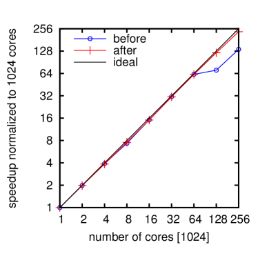
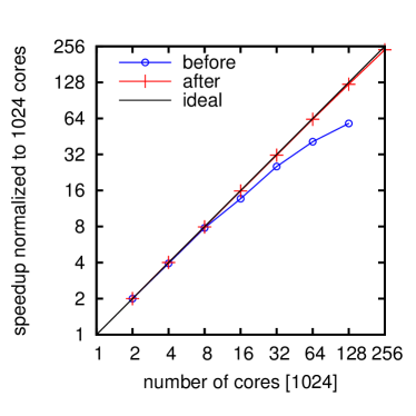
Figure 2: Strong scaling of lb3d on a Blue Gene/P machine before and after optimizations. 2 relates to a system with only one fluid component. 2 refers to a system with two fluid species and suspended particles (from Ref. bib:jens-groen-henrich-janoschek-coveney:2011 ).

In order to improve the accuracy and numerical stability of lb3d with respect to the application to the simulation of multiphase flows in porous media, recently a MRT collision model was integrated with the software. While the MRT collision algorithm is more complex than the BGK collision scheme and can cause significant performance loss when implemented naively, the increase in calculation cost can be dramatically reduced. We take advantage of two properties of the system to minimize the impact of the additional MRT operations on the code performance. First, the symmetry of the lattice allows prior calculation of the sum and difference of discrete velocities which are linear dependent, thus saving at least half of the calculation steps PhysRevE.75.066705 . Second, the equilibrium stochastical moments can be expressed as functions of the conserved properties density and velocity, thus saving the transformation of the equilibrium distributions bib:dhumieres-ginzburg-krafczyk-lallemand-luo . As such, the performance penalty could be reduced below 17%, which is close to the minimal additional cost reported in bib:dhumieres-ginzburg-krafczyk-lallemand-luo . Since in multiphase systems the relative cost of the collision scheme is further reduced, the use of the MRT scheme has even less impact on the performance and for ternary amphiphilic simulations we find a performance penalty of only 5.8%.

4.4 Parallelization on general purpose GPU arrays

The introduction of application programming interfaces such as CUDA, OpenCL, DirectCompute, and the addition of compute shaders in OpenGL, has enabled implementation of numerical methods on graphics processing hardware. When used for scientific computing, there are two primary advantages of a GPU over a CPU. Firstly, a GPU typically has a far greater number of cores. The current generation nVidia Tesla K20x has 2688 cores, while a high end Intel Xeon E-2690v2 has only 10. Second, GPUs also have a much higher memory bandwidth, with a theoretical maximum of 250 GB/s versus 59.7 GB/s for the Tesla and Xeon, respectively. It is therefore reasonable to expect that implementation of the LBM on a GPU architecture will yield significant performance improvements when compared with an equivalent multicore or cluster-based CPU implementation.

As with many CPU implementations, GPU parallelism requires the LBM domain to be decomposed into a number of equal sized blocks of lattice sites. The GPU hardware is partitioned into streaming multiprocessors (SM), each consisting of a number of cores. Each domain block is assigned to a single SM, where the lattice sites are assigned to a core and computed in parallel. The LBM computations are implemented as a kernel function which is executed on the GPU.

The performance benefits of using GPUs with the LBM are well reported. Mawson & Revell’s implementation on a single Tesla GPU achieved a peak performance of 1036 million lattice updates per second (MLUPS) Mawson2013 . Implementation of the method by Obrecht et. al. on a GPU cluster, with an older generation of GPUs, yielded speeds in excess of 8,000 MLUPS Obrecht2013259 . The work detailed by these authors reveals that writing an efficient kernel function is, however, non-trivial. Indeed, a number of issues, such as branching code, memory access, and memory consumption, must be considered when writing an efficient LBM kernel.

Branching code refers to the use of conditional statements to direct the logic of an algorithm. When a conditional statement (e.g. if statement) is executed on a CPU only the valid branch of code will be computed. This is not the case with a GPU. GPU’s are designed to be Same Instruction Multiple Data machines. This means that all cores in an SM must execute the same code which leads to two possible outcomes. In the case that all cores evaluate the statement and require the same branch of the conditional statement, only one branch is actually computed. If some cores require the first branch of the statement, and the rest require the second branch, then all cores execute both branches of the conditional statement. In the latter case, the redundant branch is computed as a null pointer operation.

There are a two situations where this branching problem is particularly relevant to the implementation of a general LBM code, namely the collision operator and boundary conditions. It is common for a general code to implement a variety of collision operators. However, the use of multiple collision operators within a single model is uncommon. In this instance it is acceptable for the collision operator selection logic to appear within the kernel. As in this case, all threads will only execute a single branch. The selection of boundary conditions at a node is also done through conditional logic. The naive approach to avoiding code branching in this scenario is to simply use two separate kernels for boundary and regular lattice sites. However, this approach requires the development of more code, and the spatial locality of lattice sites is not preserved in memory.

As was mentioned in Sec. 4.2, many LBM implementations use two data structures to store particle distribution functions. This is not optimal when using GPU hardware, as even the most recent Tesla GPUs are limited to 6GB of memory, which corresponds to approximately 34 million lattice sites when using a D3Q19 lattice. Fortunately, a number of approaches exist to remove the dual-lattice requirement. These include the Compressed Grid or Shift algorithm proposed by Pohl et al. Pohl2003 , the Swap algorithm proposed by Latt Latt2007a , and the AA Pattern algorithm proposed by Bailey et al. Bailey2009 . These approaches have been reviewed by Wittmann et al. who found that of the algorithms available, the AA Pattern algorithm proved to be the most beneficial both in terms of memory consumption and computational efficiency Wittmann2011 .

In order to achieve the maximum theoretical memory bandwidth of a GPU, memory access must be coalesced. An access pattern which is coalesced is one where, for double precision, accesses fit into segments of 128 bytes resulting in threads that read data from the same segment of the array. Various authors have presented methods to mitigate the impact of uncoalesced memory access. Toelke et al. presented a method where the streaming operation was split into two stages for a $D2Q9$ lattice, where variables are streamed first in the X-direction, and subsequently in the Y-direction Tolke2008 . Rinaldi et al. noted that uncoalesced memory reads are faster than uncoalesced writes, so they carried out propagation of the particle distribution functions in the reading step Rinaldi2012 . Streaming on read is a straightforward approach that mitigates the effect of coalesced access at no extra cost. However, recent work by Mawson & Revell has shown that techniques like the one proposed by Toelke et al. require extra processor registers, limiting the number of lattice sites which may be computed in parallel. Mawson & Revell found that, with the current generation of nVidia Tesla chips, the bandwidth reduction due to uncoalesced streaming in the LBM is at most 5% Mawson2013 .

Finally, a multi-GPU configuration can be useful when either the memory consumption of a model exceeds the available memory on a single GPU, or more computational power is required. For a code to exploit multiple GPUs another level of domain decomposition must be added in which each GPU is used to compute a subdomain. To do this, the storage strategy for lattice data must account for communication between GPUs. The solution to managing this process is found in the way in which data is marshalled between nodes in a cluster. In this case, the CPU represents a master node, the GPUs then become the slave nodes. Where the bandwidth of the PCIe x16 ports used to connect the GPU is of a similar order of magnitude to that fourteen data rate InfiniBand connection at 15.4GB/s. Though unlike an InfiniBand connection, it is not currently possible for slave nodes to access the memory of other slave nodes directly. The best strategy for this is to include ghost nodes so that race conditions are avoided during the streaming of particle distribution functions across the subdomain boundary. The master node, or CPU, is then used to manage data transfer between devices.

5 Applications

In this section the ability of the discussed multiphase models to capture the relevant physics of multiphase flow problems in porous media is demonstrated. This is undertaken using baseline tests of two-dimensional flow in synthetic porous media.

5.1 The color gradient model

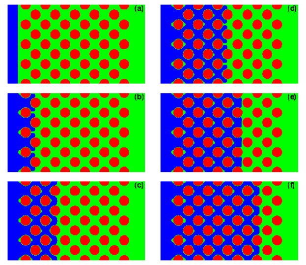
Figure 3: (Color online) Time evolution of non-wetting fluid displacing the wetting fluid for $Ca=5\times 10^{-3}$ and $M=\frac{1}{10}$ at timesteps: (a) 0; (b)16000; (c)34000; (d)48000; (e)60000; and (f)74000.

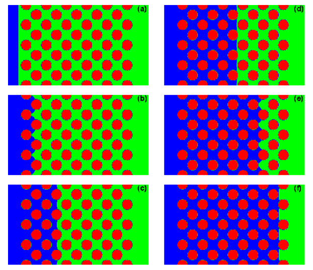
Figure 4: (Color online) Time evolution of wetting fluid displacing the non-wetting fluid for $Ca=5\times 10^{-3}$ and $M=4$ at timesteps: (a) 0; (b)8000; (c)18000; (d)26000; (e)38000; and (f)46000.

In the current example, no-slip boundary conditions at solid walls are implemented by a simple bounce-back rule Latva-Kokko2005a . The wettability of the solid walls can be imposed by assuming that the solid wall is a mixture of two fluids, thus having a certain value of the phase field Latva-Kokko2005a ; Liu2011 . The interfacial force term in Eq. (17) becomes dependent on the properties of the neighboring solid lattice sites, resulting in a special case of the wetting boundary condition. The assigned value of the phase field at sites neighboring the wall sites can be used to modify the static contact angle of the interface. Figs. 3 and 4 give the time evolution of interface at $Ca=0.005$ for drainage process with $M=\frac{1}{10}$ and imbibition process with $M=4$ in a 2D pore network, consisting of a uniform distribution of circular grains. Here, the capillary number ($Ca$) relates viscous to capillary forces and is defined as $Ca=u_{in}\eta_{in}/\sigma$, where $u_{in}$ and $\eta_{in}$ are the mean velocity and dynamic viscosity of the displacing fluid at the inlet, respectively. The viscosity ratio, $M$, is defined as the ratio of non-wetting fluid viscosity to the wetting fluid viscosity: $M=\eta_{nw}/\eta_{w}$. In the drainage process, the non-wetting fluid advances in a piston-like manner in the pore throats. It can be clearly observed that there is one small blob of defending fluid trapped near the rear stagnant point for each solid grain. Similar trapped blobs are also found at the front stagnant point for the first column of grains. These trapped blobs of defending fluid are attributed to low flow velocity and high pressure at the front and rear stagnant points, so that the wetting fluid cannot be completely drained out before the advancing interfaces of non-wetting fluid coalesce or touch the surface of solid grains. However, the defending fluid is completely drained out in the imbibition process, where the interface advances in a more stable manner, and the solid surface favors the invading fluid but repels the defending fluid.

5.2 Inter-particle potential model

The inter-particle potential model was used extensively for various multiphase flow problems, see Refs. Martys1996 ; Schmieschek2011 ; Pan2004 ; Sukop2004 ; Li2005 ; Huang2009a ; Porter2009 ; Parmigiani2011 ; Dong2011 ; Ghassemi2011 ; Mukherjee2011 ; Middleton2012 ; Dou2013 ; bib:jens-venturoli-coveney:2004 ; bib:jens-harvey-chin-venturoli-coveney:2005 , because of its simplicity and easy implementation. Pan et al. Pan2004 used the MCMP inter-particle potential model to simulate two-phase flow in a porous medium comprised of a synthetic packing with a relatively uniform distribution of spheres. They achieved good agreement between the measured hysteretic capillary pressure saturation relations and the lattice Boltzmann simulations when comparing entry pressure, displacement slopes, irreducible saturation, and residual entrapment. The hysteresis was also found by Sukop and Or Sukop2004 who adopted the SCMP inter-particle potential model to simulate the liquid-vapor distributions in a porous medium based on two-dimensional imagery of a real soil. Porter et al. Porter2009 further emphasized the importance of the wetting-nonwetting interfacial area. They adopted the MCMP inter-particle potential model to study the hysteresis in the relationship between capillary pressure, saturation, and interfacial areas in a three-dimensional glass bead porous medium obtained by computed micro-tomographic (CMT) image data.

The inter-particle potential model has also been used to determine relative permeabilities Li2005 ; Ghassemi2011 ; Huang2009a ; Dou2013 . Effects of capillary number, wettability, and viscosity ratio, as well as the porous structures on the relative permeability were investigated in detail. However, the original inter-particle potential model suffers from some limitations, including large spurious velocities in the vicinity of the fluid-fluid interface, viscosity-dependent equilibrium density and interfacial tension, and numerical instability for large viscosity or density ratios. In the SCMP model, the kinematic viscosity is fixed, and the density ratio is limited to the order of 10. In the MCMP model, the viscosity and density ratios are typically restricted to no more than 5 and 3, respectively.

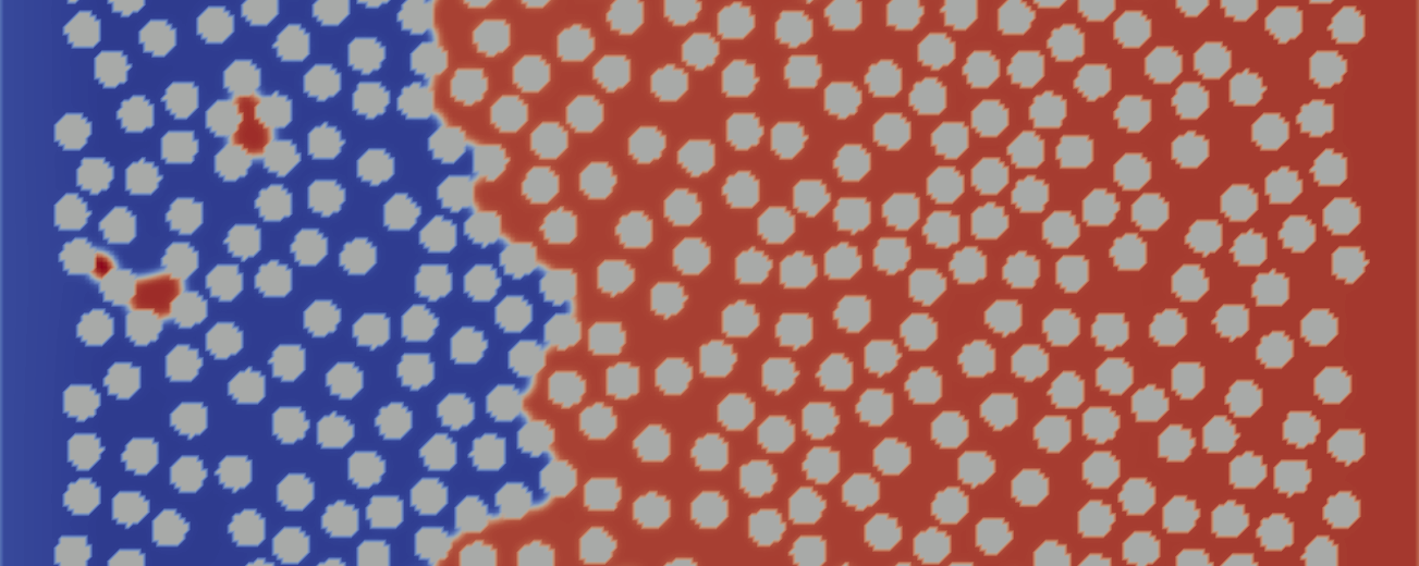
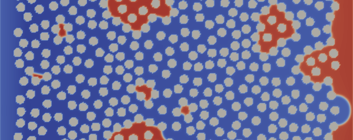
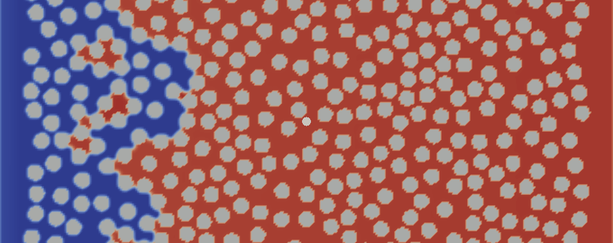
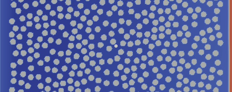
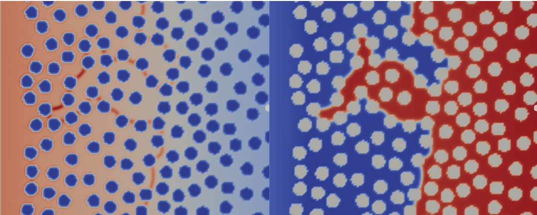
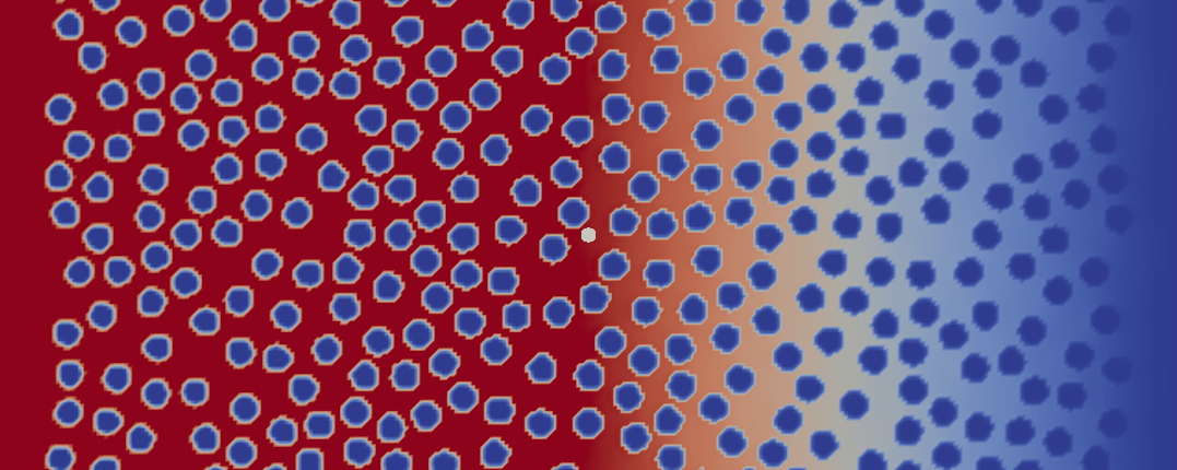
Figure 5: Snapshots of fluid density fields after imbibition simulation using an inter-particle potential binary (ternary) fluid model in a pseudo-2d porous medium, varying different parameters. 5: Comparison of stable density distributions of the displaced (oil) component after 500,000 timesteps varying an applied body force (pressure gradient) in lattice units between $F=2\cdot 10^{-4}$ and $F=4\cdot 10^{-4}$ in a neutrally wetting system. 5: Comparison of stable density distributions of the displaced (oil) component after 500,000 timesteps varying the contact angle of the displaced component between $\Theta=17^{\circ}$ and $\Theta=163^{\circ}$, applying a constant body force of $F=4\cdot 10^{-4}$. 5:Illustration of the surfactant component density field after 100,000 timesteps. Left: Surfactant component density (left) vs. displaced (oil) component density (right) injecting a surfactant concentration $c_{\text{S}}=0.2$ together with the displacing fluid into a neutrally wetting system, applying a constant body force of $F=4\cdot 10^{-4}$. Right: Surfactant component density field injecting a surfactant concentration $c_{\text{S}}=0.5$ together with the displacing fluid into a neutrally wetting system, applying a constant body force of $F=4\cdot 10^{-4}$.

Fig. 5 illustrates simulations of imbibition into a pseudo-2D porous medium using a ternary fluid mixture model as described in Section 3, equations (29-3.2). The qualitative effect of variation of different system parameters on the stable configuration is being investigated. The system consists of a 512$\times$1280 lattice with randomly placed cylinders, which assures a minimum required resolution of the smallest pores. Re-coloring boundary conditions are applied at the inlet and outlet so that fluid of one component crossing the periodic boundary is added to the second component when appearing on the other side of the system. The surfactant follows standard periodic boundary conditions. The coupling parameters of the inter-particle potential model are kept fixed at $G_{c}=0.1$, $G_{k,s}=-0.006$, and $G_{s,s}=-0.003$.

Fig. 5 shows a comparison of the stable density distributions of the displaced (oil) component after 500,000 timesteps. Here, the applied body force, which is directly proportional to the pressure gradient, is in lattice units varied between $F=2\cdot 10^{-4}$ (left) and $F=4\cdot 10^{-4}$ (right). No surfactant is present and a contact angle of $\Theta=90^{\circ}$ corresponding to neutral wetting is applied. Between the considered values of forcing a transition from halted to complete filling in the stable state of the system by the injected (water) component is observed.

Again, Fig. 5 shows a comparison of the stable density distributions of the displaced (oil) component after 500,000 timesteps. Here, however, the driving body force is kept fixed at $F=4\cdot 10^{-4}$ and the contact angle of the displaced (oil) component is varied between $\Theta=17^{\circ}$ and $\Theta=163^{\circ}$. The strongly wetting case as depicted on the left reverts the effect of stronger pressure and the system again becomes stable in a partially filled state. As to be expected for the strongly dewetting case shown on the right, the displaced (oil) component is completely flushed out of the system.

Fig. 5 contains simulation snapshots after 100,000 timesteps. The driving force and contact angle are kept constant at $F=4\cdot 10^{-4}$, and $\Theta=90^{\circ}$, respectively. A surfactant component is being added to the invading fluid (water) component. On the left hand side for injecting a surfactant concentration $c_{\text{S}}=0.2$, concurrent density fields of the surfactant component (left) and the displaced (oil) component are plotted side by side. The surfactant is agglomerating at the interface as denoted by the dark red spots. For this concentration, a relatively sharp interface is conserved. On the contrary, for a concentration of the surfactant component in the invading fluid of $c_{\text{S}}=0.5$, a transition to a diffusive regime can be observed on the right hand side. It is noteworthy that the interfacial width in the diffusive regime is of the order of tens or even hundreds of lattice sites. In real life conditions, this should still correspond to length scales of several nanometres or tens of nanometres only, which depicts a limitation of diffuse interface models for porous media flows.

These examples clearly demonstrate the ability of the amphiphilic model to qualitatively study the effect of surfactants on imbibition in porous media, which is of relevance for enhanced oil recovery applications.

5.3 Free-energy model

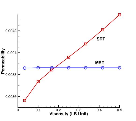
Figure 6: (Color online) Comparison of the permeability calculated based on MRT and SRT models with various viscosities for single-phase flow through a periodic body-centered cubic array of spheres, whose porosity is $\varepsilon=0.394$.

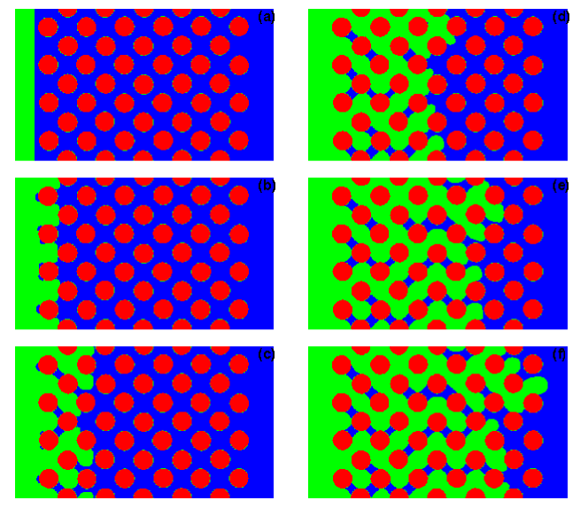
Figure 7: (Color online) Time evolution of less viscous non-wetting fluid displacing more viscous wetting fluid for $Ca=5\times 10^{-4}$, $M=1/10$ and $\theta=135^{\circ}$ at timesteps (a) 0, (b) 200000, (c) 400000, (d) 800000, (e) 1100000, and (f) 1300000 using MRT free energy model of potential form.

It has been widely demonstrated that with the bounce-back boundary condition at the solid walls, the SRT LBM produces viscosity-dependent permeability in porous media, while the viscosity-independent solution can be produced by MRT Pan2006 ; Hao2009a . This can be clearly seen in Fig. 6, which plots the permeability as a function of viscosity for the single-phase flow through a body-centered cubic array of spheres. To produce viscosity-independent permeability, we implement the free-energy model of potential form using MRT with two independent relaxation times (i.e. the two-relaxation-time algorithm Pan2006 ; Hao2009a ). This model is applied to simulate the less viscous non-wetting fluid displacing the wetting fluid in a pore network with slightly irregular distribution of cylinder center (which is obtained by adding randomly small perturbation to the regularly distributed position). Fig. 7 gives the displacement processes for the periodic boundary conditions at the upper and lower boundaries. Similar to the observations in the color gradient model, we can clearly see some small blobs trapped near the front sides for the first column of solid grains. Also, the trapped small blobs can dissolve very quickly as the simulations progress. Actually, the dissolution of small droplets/bubbles is a typical phenomenon in many diffuse-interface models (e.g. the phase-field or free-energy model). The droplet dissolution is attributed to two factors. The first is that a multiphase system is always evolving towards the direction of decreasing free energy in the free-energy model, and the system with the droplets completely dissolved has a lower free energy than the one with two-phase coexistence, so small droplets are prone to dissolve Sman2008 . The second is that the Cahn-Hilliard equation can conserve the total mass of the system but cannot conserve the mass for each component/fluid. Several methods have been proposed for reducing the rate of dissolution in some simple systems, but more efforts are still required to obtain physically meaningful numerical results in a large and complex porous media, where the slim fingers may be dynamically evolving and sometimes unstable.

5.4 Mean-field theory model

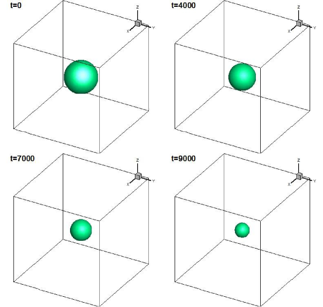
Figure 8: (Color online) Time evolution of a liquid droplet with radius $R=10$ in a stationary gas phase. The size of computational domain is $60\times 60\times 60$. The densities of liquid and gas are 1 and 0.25, and the relaxation times for both fluids are taken 0.53. Other parameters can be found in Ref. Premnath2007 .

The mean-field theory model has been implemented by Premnath and Abraham Premnath2007 with the MRT algorithm in order to achieve better numerical stability. Using this MRT model, we also simulated a 3D stationary bubble in a liquid domain with periodic boundary conditions applied at all the boundaries. When using the same parameters as given in Premnath2007 , we found that good results can be obtained without bubble dissolution. However, as the bubble size is decreased, it can be observed that the bubble can quickly dissolve, which is shown in Fig. 8. A fast dissolution is disastrous for obtaining reliable simulation results. Fakhari and Rahimian Fakhari2010a also noticed the dissolution problem in their two-dimensional axisymmetric simulations, and they suggested to take $a=12.75RT$, which can effectively reduce diffusion of different phases into each other. However, we found that this improvement is not very effective in 3D stationary bubble tests.

5.5 Stabilized diffuse-interface model

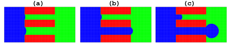
Figure 9: (Color online) Injection of a non-wetting gas into two parallel capillary tubes with the pressure difference $\Delta p$ of (a) $4\times 10^{-5}$, (b) $6\times 10^{-5}$, and (c) $8\times 10^{-5}$. The capillary pressure is $P_{c_{1}}=7.1\times 10^{-5}$ for the upper tube and $P_{c_{2}}=4.7\times 10^{-5}$ for the lower tube (reproduced from Ref. Liu2013 ).

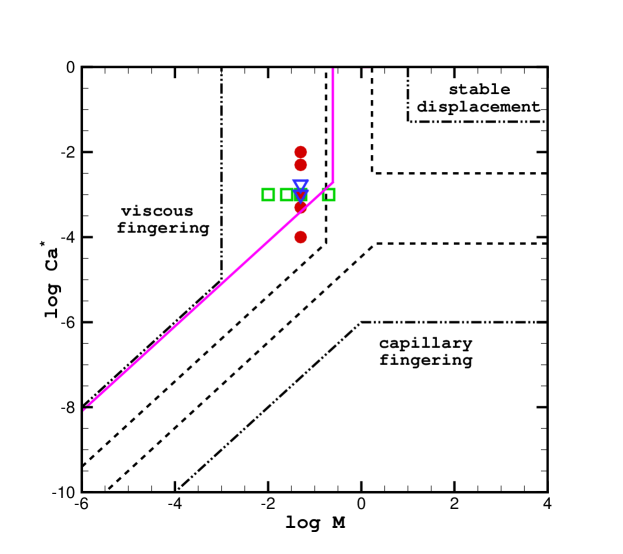
Figure 10: (Color online) $\log Ca^{*}-\log M$ phase diagram indicating the fluid displacement patterns and the locations of the numerical simulations given by Liu et al. Liu2013 (represented by discrete symbols) for drainage displacement, where the capillary number $Ca^{*}$ is defined by $Ca^{*}=\frac{u_{in}\eta_{in}}{\sigma\cos(\theta)}$. The stability zones bounded by black dash-dot-dotted, black dashed, and pink solid lines, are obtained by Lenormand et al. Lenormand1988 , Zhang et al.Zhang2011a , and the simulations of Liu et al., respectively (reproduced from Ref. Liu2013 ).

Here, we demonstrate that the stabilized diffuse-interface model is most suitable to simulate flow problems with high density ratio. No-slip boundary conditions are applied at solid walls using the bounce-back scheme Lee2010 . For a straight solid wall, the method of Lee and Liu Lee2010 can be employed to impose the wetting boundary condition. Recently, a wetting boundary treatment was proposed for concave and convex corners, which can be extended to more complicated geometries with curved boundaries represented by a staircase approximation Liu2013 . With the proposed wetting boundary treatment, Liu et al. Liu2013 have simulated the injection of a non-wetting gas through two parallel capillary tubes (the widths of the upper and lower capillaries are $r_{1}$ and $r_{2}$, and $r_{1}<r_{2}$, leading to the capillary pressure $p_{c1}>p_{c2}$.) at several different $\Delta p$, where $\Delta p$ is the pressure difference between the inlet and outlet. As expected, the findings were that when $\Delta p$ is smaller than $p_{c2}$ (Fig. 9(a)), the invading gas cannot enter both capillary tubes, when $\Delta p$ is between $p_{c2}$ and $p_{c1}$ (Fig. 9(b)), the gas only flows into the large capillary tube, and when the pressure difference is increased to $\Delta p>p_{c1}$ (Fig. 9(c)), the gas flows into both capillary tubes, but the displacement is much faster in the large capillary tube. This displacement behavior is consistent with the principle of pore-network simulators Lenormand1988 , which suggests that this HDR model is able to capture capillary effects and reproduce correct displacement behavior. The stabilized diffuse-interface model was also used to simulate gas displacement of liquid in a homogenous two-dimensional pore network consisting of uniformly spaced square obstructions. The effect of capillary number, viscosity ratio, surface wettability, and Bond number was studied systematically. Similar to previous experimental observations Lenormand1988 , three different regimes, namely stable displacement, capillary fingering, and viscous fingering, were identified in the drainage displacement, and all of them are strongly dependent upon the capillary number, viscosity ratio, and Bond number. The simulation results shown in the two-dimensional phase diagram (see Fig. 10) denote that the viscous fingering regime covers a region markedly different from those obtained in previous numerical and experimental studies Lenormand1988 ; Zhang2011a . The difference is because the boundaries of the regimes in the phase diagram are strongly dependent on the configuration of the pore network, and also upon 3D effects, which are neglected in 2D simulations but can play a non-trivial role for determining the displacement behavior in micromodel laboratory experiments.

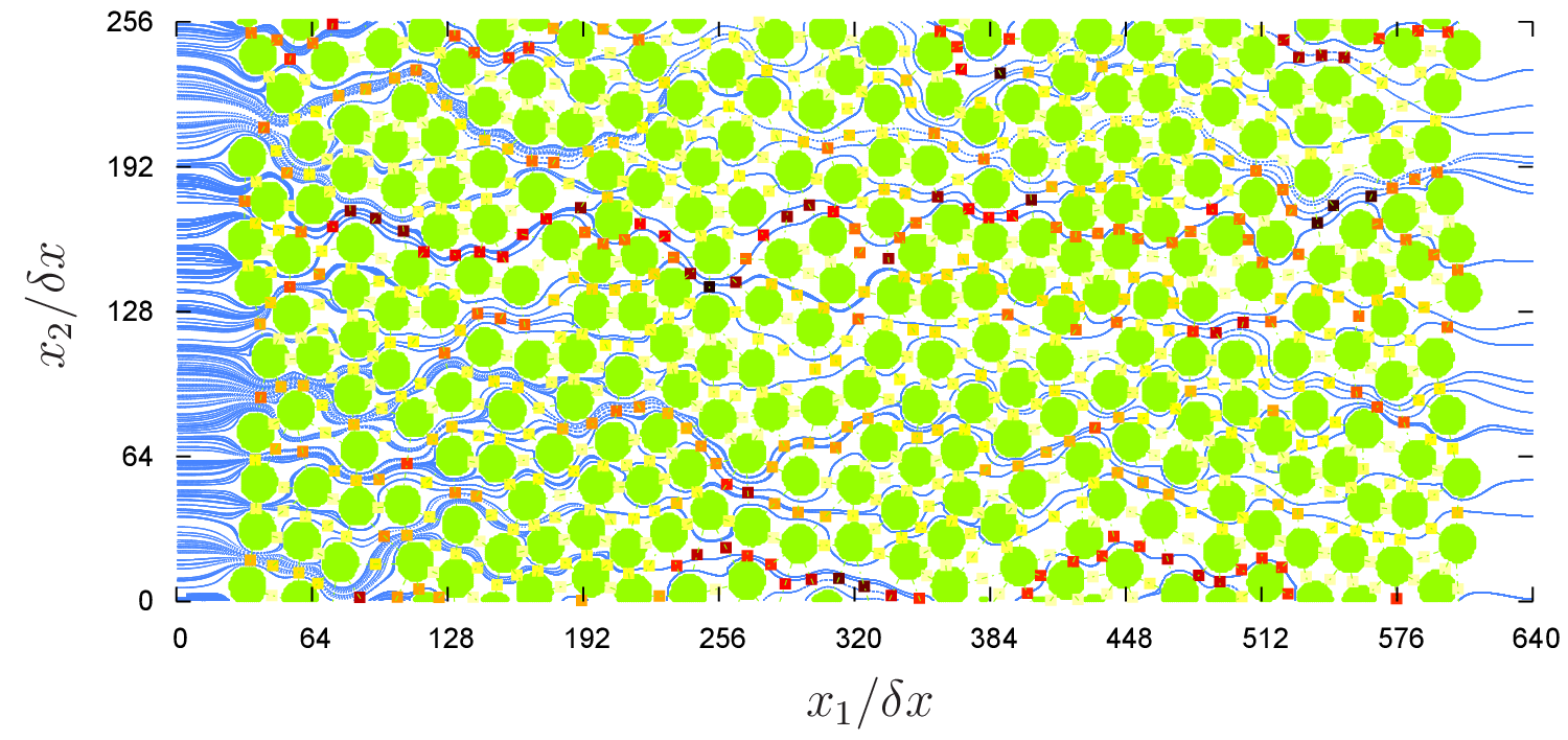
(a) tracer

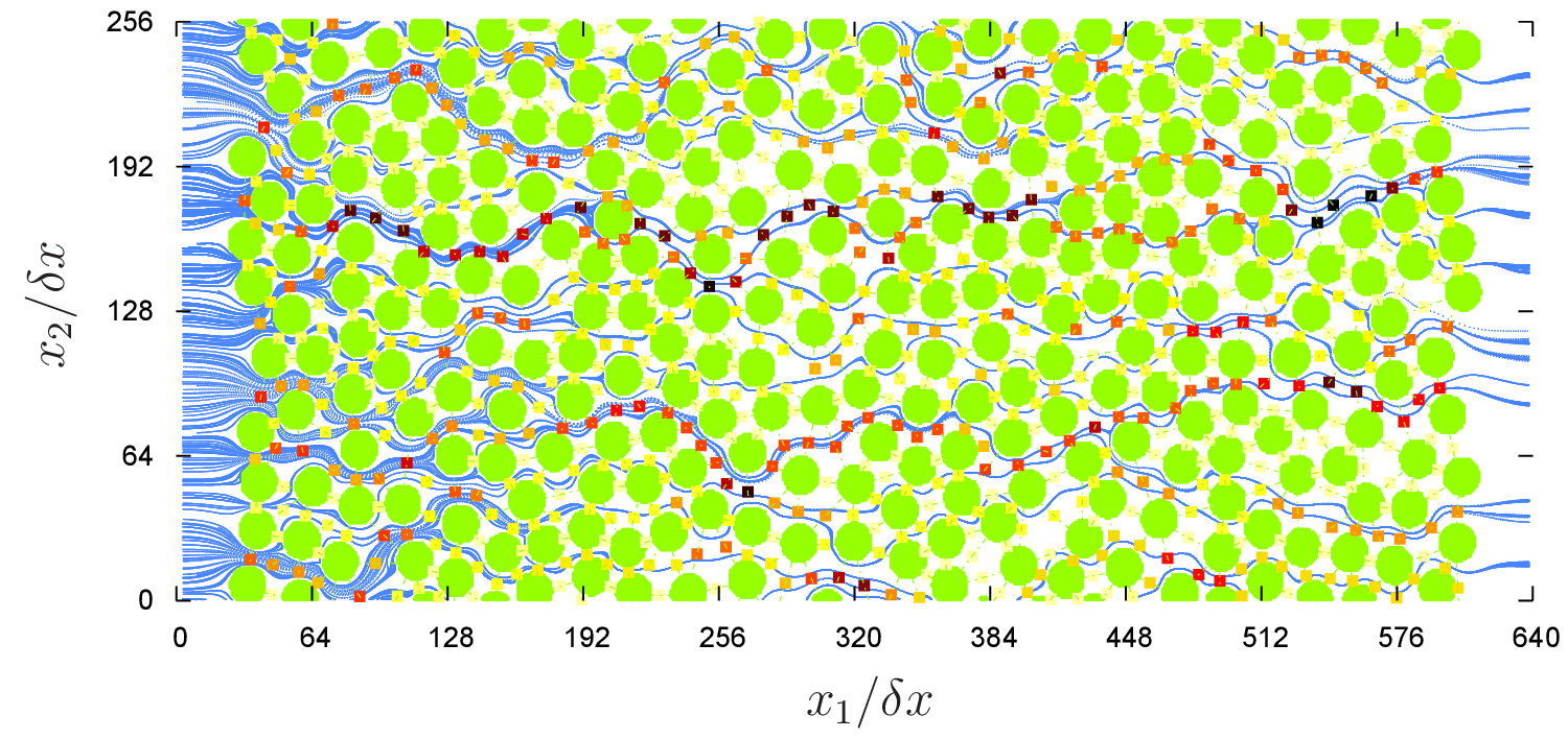
(b) $r_{\rm p}=1.6$

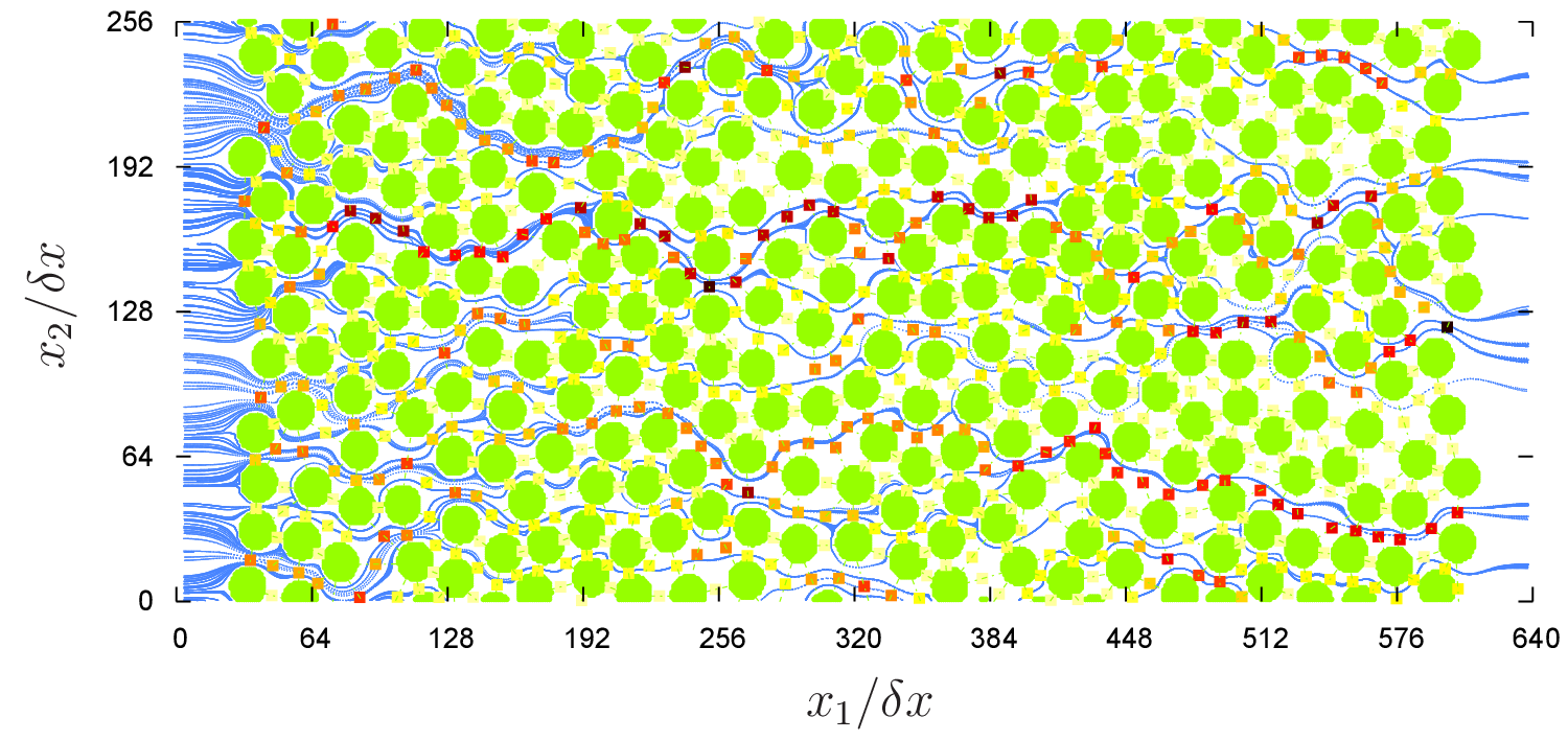
(c) $r_{\rm p}=2.1$

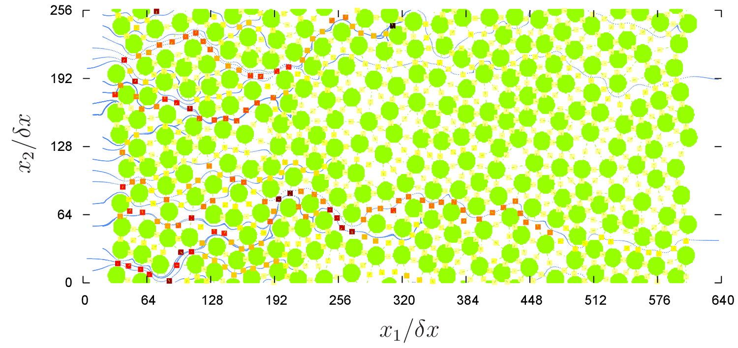
(d) $r_{\rm p}=2.6$

Figure 11: Time averaged steady state particle trajectories (blue lines) in a porous medium made by randomly placed cylinders (green circles). Between each pair of neighbor cylinders a colored square is located showing the probability of a particle to flow through. The radius of the particles $r_{\mathrm{p}}$ is varied between zero (tracers) and $2.6$.

5.6 Particle suspensions

Particle suspensions in porous media are relevant in many processes such as fines migration Leonardi2012a ; Leonardi2012b , sand liberation Boutt2011 , catalysis, heap-leaching, filtration, fertilization, and contaminant spreading in the subsoil. In these applications, relevant questions involve the possibility of sealing of porous media, segregation, or the formation of particle clusters and their influence on the transport properties inside the porous structure. While for some applications one might like to optimize a porous medium so as to allow almost all particles to pass (e.g. reactors and catalysts), other applications demand a perfect trapping of all particles (e.g. filters).

Coupled lattice Boltzmann and discrete element/molecular dynamics algorithms are a powerful tool to simulate such systems since they leverage the strengths of two numerical algorithms. As demonstrated in the previous sections, the LBM is well suited to describe (multiphase) fluid flow in complex geometries. Particle based methods, on the other hand, allow the description of interacting particles by solving Newton’s equations of motion. Here, we limit ourselves to non-interacting point-wise particles (tracers) and massive spherical particles which only interact through hydrodynamic and Hertz forces in order to mimic hard spheres. The massive particles have the same mass density as the fluid. However, this is not a general restriction of the algorithm. Electrostatic, van der Waals, magnetic, or any other kind of interactions can be used in the same way as in classical molecular dynamics. We also ignore te effect of diffusion on tracer particles which could be taken care of by adding a diffusive term Yang:2013b .

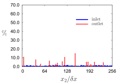
(a) tracer

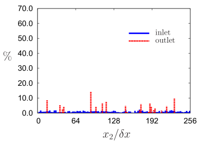
(b) $r_{\mathrm{p}}=1.6$

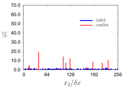
(c) $r_{\mathrm{p}}=2.1$

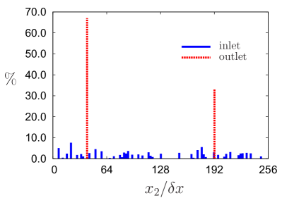
(d) $r_{\mathrm{p}}=2.6$

Figure 12: Histogram of the particle positions at the inlet and outlet plane of the model porous medium for tracers and massive particles of radius $r_{\mathrm{p}}=1.6$, $r_{\mathrm{p}}=2.1$, and $2.6$, respectively.

Our system of interest is again a pseudo-2D porous medium made of randomly placed cylinders as shown in Fig. 11. The system size is $256\times 640$ and the fluid is driven using pressure boundary conditions in $x_{1}$ direction. Particles leaving the simulation domain at the outlet in $x_{1}$ direction re-enter at the inlet, but at a randomly chosen $x_{2}$ position. All other boundaries are periodic. These particles only interact with walls by means of lubrication forces and a very short range repulsive force. When the simulation has reached a steady state, we record the trajectories of 1000 tracer particles or 100 massive particles being transported by the flow. Figs. 11(a) to 11(d) depict these trajectories for tracers and particles with radius, $r_{\mathrm{p}}=1.6$, $2.1$, and $2.6$, respectively. It can be clearly seen that even for tracer particles preferable paths exists. This is due to high local flow velocities which have their origin in the particular arrangement of the cylinders. When increasing the particle radius, the number of preferable paths reduces for several reasons. First, particles with an extended size are only able to pass through pores which are larger than the particle diameter. Second, particles might block small pores rendering the area behind it practically inaccessible for all further particles flowing in. This effectively leads to a dynamic rearrangement of the flow field and based on that the preferable paths the particles tend to follow will change as well.

This explanation is underlined by Figures 12 and 13. Fig. 12 depicts histograms of $x_{2}$ positions where particles enter at the inlet (randomly chosen) and where they leave the system at the outlet. Interestingly, the tracers and the small particles with $r_{\mathrm{p}}=1.6$ show a similar number of preferred outlet positions. However, these are differently distributed because the massive particles also influence the flow field – even though they are sufficiently small to pass almost all pore throats. The histogram for the largest particles with $r_{\mathrm{p}}=2.6$ shows that only three possible percolating paths seem to be accessible, while all others include pore throats which are smaller than the particle diameter.

By averaging over all particles $i$ the recorded trajectories can be used to compute the mean square displacement $\mathrm{mqd}(t)=\left<(r_{i}(t)-r_{i}(t=0))^{2}\right>_{i,t}$. $\mathrm{mqd}(t)$ is shown for the different particle species in Fig. 13. It can be concluded that small massive particles can be transported through the porous medium almost as efficiently as tracers – even though they follow different preferable paths as demonstrated by the histograms in Fig. 12. For larger particles, however, the probability that some of them get stuck in small pores grows leading to a substantial reduction of the mean square displacement.

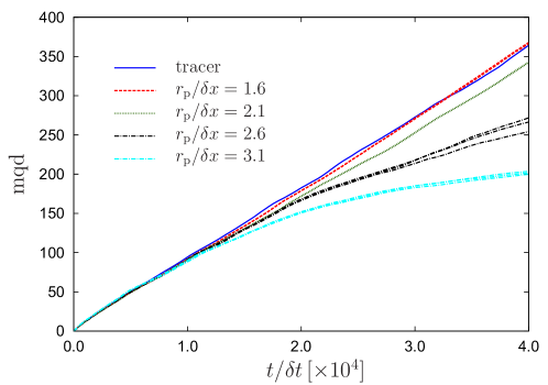
Figure 13: Mean square displacement of the particles inside the porous medium for different particle sizes.

6 Conclusion

In this article we provided a comprehensive overview and literature review on lattice Boltzmann modelling of multiphase flow with a particular focus on porous media applications. We introduced several algorithmic extensions of the LBM to describe multiple fluid phases or solid phases suspended in fluid. Their individual advantages and disadvantages were discussed based on simple example cases.

To guide readers to choose appropriately among the different LBM formulations for multiple fluid phases reviewed above, Table 1 gives a brief summary of their capabilities which are examined through a series of comparisons, including (i) the ability of modeling the interfacial tension, which can be given directly in the model or should be obtained numerically through the static bubble test based on the Laplace’s law, (ii) the magnitude of maximum spurious velocities in the static bubble test, (iii) dissolution rate for small droplets/bubbles, (iv) the highest density ratio that can be achieved, (v) the highest kinematic viscosity ratio that can be achieved, and (vi) the computing cost. As can be seen from Table 1, each lattice Boltzmann multiphase model has its own advantages and limitations, and it is not possible to state that one model is definitely preferred to another. However, it will be beneficial to be aware of and carefully consider the following points, especially when the LBM is chosen for pore-scale simulation of multiphase flows in porous media:

(1) The stabilized diffuse-interface model can almost eliminate the spurious velocities to round-off error, free-energy and color gradient models produce larger spurious velocities and the inter-particle potential model has largest spurious velocities;

(2) Small droplets/bubbles are expected to dissolve for stabilized diffuse-interface model, free-energy model and mean-field theory model, and the dissolution rate is fastest for the mean-field model;

(3) The stabilized diffuse-interface model is most suitable to simulate flow problems with high density ratio, while the color gradient model is most suitable to simulate flows with moderate/high viscosity ratio;

(4) The free-energy model of potential form can produce smaller spurious velocities than its stress/pressure form, thus leading to the correct equilibrium contact angles when the binary fluids have different viscosities.

Table 1: A summary of the capabilities of several lattice Boltzmann multiphase models.

		Models
	Inter-particle potential	Color	Free-energy
Interfacial tension	static bubble test	can be given	can be given
	is required	directly	directly
Spurious currents	large	medium	small
Dissolution for tiny	small	very small	large
bubbles/droplets
Density ratio	1000†	1000∗	1
Kinematic viscosity	1000‡	1000	up to 8
ratio
Computing cost	‘average’	‘average’	‘average’
		Models
	Mean-field theory	Stabilized diffuse-interface
Interfacial tension	static bubble	can be given
	test is required	directly
Spurious currents	medium	very small
Dissolution for tiny	very large	medium
bubbles/droplets
Density ratio	up to around 15	1000
Kinematic viscosity	unknown	unknown
ratio
Computing cost	greater	large∗∗

^† Achieved in static bubble test with both SCMP Yuan2006 and MCMP Bao2013 models using equations of state different from the original Shan-Chen model.
^‡ Achieved in static bubble test and two-phase cocurrent flow between two parallel plates with the MCMP model, using higher-order isotropy in the fluid-fluid interfacial terms, explicit forcing scheme, and multiple relaxation times Porter2012 .
^∗ Achieved in static bubble test using the color gradient model presented in  Liu2012a .
^∗∗ The normal direction at each boundary node should be identified, and high-order approximations to derivatives are needed.

- (1) R. Hilfer, Adv. Chem. Phys. XCII (1996)
- (2) R. Hilfer, Phys. Rev. B 45, 7115 (1992)
- (3) K.L. Dixon, R.L. Nichol, Env. Geosci. 12, 279 (2005)
- (4) G.W. Gee, F.Z. Zhang, A.L. Ward, Vadose Zone J. 2, 627 (2003)
- (5) A. Koponen, M. Kataja, J. Timonen, Phys. Rev. E 56, 3319 (1997)
- (6) P. Garrido, F. Concha, R. Bürger, Int. J. Mineral Process 72, 57 (2003)
- (7) M.T. Balhoff, S.G. Thomas, M.F. Wheeler, Comput. Geosci. 12, 15 (2008)
- (8) M. Blunt, P. King, Transp. Porous Med. 6, 407 (1991)
- (9) S. Bryant, M. Blunt, Phys. Rev. A 46, 2004 (1992)
- (10) M.S. Al-Gharbi, M.J. Blunt, Phys. Rev. E 71, 016308 (2005)
- (11) P. Valvatne, M. Piri, X. Lopez, M. Blunt, Transp. Porous Med. 58, 23 (2005)
- (12) M. Piri, M.J. Blunt, Phys. Rev. E 71, 026301 (2005)
- (13) M.J. Blunt, B. Bijeljic, H. Dong, O. Gharbi, S. Iglauer, P. Mostaghimi, A. Paluszny, C. Pentland, Adv. Water Resour. 51, 197 (2013)
- (14) V. Joekar-Niasar, S. Hassanizadeh, A. Leijnse, Transp. Porous Media 74, 201 (2008)
- (15) V. Joekar-Niasar, S. Hassanizadeh, H. Dahe, J. Fluid Mech. 655, 38 (2010)
- (16) A. Raoof, S. Hassanizadeh, Transp. Porous Media 81, 391 (2010)
- (17) Z. Jiang, K. Wu, G. Couples, M. van Dijke, K. Sorbie, J. Ma, Water Res. Research 43, (2007)
- (18) C. Hirt, B. Nichols, J. Comput. Phys. 39, 201 (1981)
- (19) W.J. Rider, D.B. Kothe, J. Comput. Phys. 141, 112 (1998)
- (20) D. Gueyffier, J. Li, A. Nadim, R. Scardovelli, S. Zaleski, J. Comput. Phys. 152, 423 (1999)
- (21) A. Ferrari, I. Lunati, Adv. Water Resour. 57, 19 (2013)
- (22) S. Osher, J.A. Sethian, J. Comput. Phys. 79, 12 (1988)
- (23) M. Sussman, E. Fatemi, P. Smereka, S. Osher, Comput. Fluids 27, 663 (1998)
- (24) S. Osher, R.P. Fedkiw, Level sets methods and dynamic implicit surfaces (Springer, 2003)
- (25) R. Benzi, S. Succi, M. Vergassola, Phys. Rep. 222 (1992)
- (26) Y.H. Qian, D. d’Humières, P. Lallemand, Europhys. Lett. 17, 479 (1992)
- (27) S. Succi, The lattice Boltzmann equation for fluid dynamics and beyond (Oxford University Press, 2001)
- (28) A. Cancelliere, C. Chang, E. Foti, D.H. Rothman, S. Succi, Phys. Fluids 2, 2085 (1990)
- (29) B. Ferréol, D.H. Rothman, Transp. Porous Media 20, 3 (1995)
- (30) A.J. Briant, A.J. Wagner, J.M. Yeomans, Phys. Rev. E 69, 031602 (2004)
- (31) A.J. Briant, J.M. Yeomans, Phys. Rev. E 69, 031603 (2004)
- (32) H.Y. Chen, D. Jasnow, J. Viñals, Phys. Rev. Lett. 85, 1686 (2000)
- (33) Q. Kang, D. Zhang, S. Chen, Phys. Fluids 14, 3203 (2002)
- (34) Q. Kang, D. Zhang, S. Chen, Adv. Water Resour. 27, 13 (2004)
- (35) Q. Kang, D. Zhang, S. Chen, Journal of Fluid Mechanics 545, 41 (2005)
- (36) S. Chen, G.D. Doolen, Annu. Rev. Fluid Mech. 30, 329 (1998)
- (37) J. Harting, M. Harvey, J. Chin, M. Venturoli, P. Coveney, Phil. Trans. R. Soc. Lond. A 363 (2005)
- (38) J. Harting, T. Zauner, A. Narváez, R. Hilfer, in High Performance Computing in Science and Engineering ’08, ed. by W. Nagel, D. Kröner, M. Resch (Springer, 2008)
- (39) A. Narváez, J. Harting, Advances in Applied Mathematics and Mechanics 2, 685 (2010)
- (40) A. Narváez, T. Zauner, F. Raischel, R. Hilfer, J. Harting, J. Stat. Mech: Theor. Exp. 2010, P211026 (2010)
- (41) N.S. Martys, J.G. Hagedorn, D. Goujon, J.E. Devaney, in Developments in X-Ray Tomography II, Proceeding of SPIE, vol. 3772 (1999), vol. 3772, p. 205
- (42) C. Manwart, U. Aaltosalmi, A. Koponen, R. Hilfer, J. Timonen, Phys. Rev. E 66, 016702 (2002)
- (43) J. Harting, M. Venturoli, P. Coveney, Phil. Trans. R. Soc. Lond. A 362, 1703 (2004)
- (44) B. Ahrenholz, J. Tölke, M. Krafczyk, Int. J. Comp. Fluid Dyn. 20, 369 (2006)
- (45) A. Koponen, D. Kandhai, E. Hellén, M. Alava, A. Hoekstra, M. Kataja, K. Niskanen, P. Sloot, J. Timonen, Phys. Rev. Lett. 80, 716 (1998)
- (46) U. Frisch, B. Hasslacher, Y. Pomeau, Phys. Rev. Lett. 56, 1505 (1986)
- (47) S. Wolfram, J. Stat. Phys. 45, 471 (1986)
- (48) G.R. McNamara, G. Zanetti, Phys. Rev. Lett. 61, 2332 (1988)
- (49) F.J. Higuera, J. Jiménez, EPL 9, 663 (1989)
- (50) R. Benzi, S. Succi, M. Vergassola, Physics Reports 222, 145 (1992)
- (51) H. Chen, S. Chen, W.H. Matthaeus, Phys. Rev. A 45, R5339 (1992)
- (52) Y.H. Qian, D. d’Humiéres, P. Lallemand, Europhys. Lett. 17, 479 (1992)
- (53) P.L. Bhatnagar, E.P. Gross, M. Krook, Phys. Rev. 94, 511 (1954)
- (54) R. Liboff, Kinetic theory: classical, quantum, and relativistic descriptions (Prentice-Hall, 1990)
- (55) S. Chapman, T.G. Cowling, The mathematical theory of non-uniform gases, 2nd edn. (Cambridge University Press, 1952)
- (56) X. He, L.S. Luo, Phys. Rev. E 56 (1997)
- (57) G. McNamara, G. Zanetti, Phys. Rev. Lett. 61, 2332 (1988)
- (58) S. Chen, G.D. Doolen, Annu. Rev. Fluid 30, 329 (1998)
- (59) C.K. Aidun, J.R. Clausen, Annu. Rev. Fluid 42, 439 (2010)
- (60) P. Lallemand, L.S. Luo, Phys. Rev. E 61, 6546 (2000)
- (61) F.J. Higuera, S. Succi, R. Benzi, Europhys. Lett. 9, 345 (1989)
- (62) D. d’Humiéres, Rarefied gas dynamics- Theory and simulations (The American Institute of Aeronautics and Astronautics, 1992), pp. 450–458
- (63) A.J.C. Ladd, J. Fluid Mech. 271, 285 (1994)
- (64) D. d’Humiéres, Phil. Trans. R. Soc. Lond. A 360, 437 (2002)
- (65) I. Ginzburg, Adv. Water Res. 28, 1171 (2005)
- (66) I. Ginzburg, D. dâHumiéres, A. Kuzmin, J. Stat. Phys 139, 1090 (2010)
- (67) A.J.C. Ladd, Phys. Rev. Lett. 70, 1339 (1993)
- (68) B. Dünweg, U. Schiller, A. Ladd, Phys. Rev. E 76 (2007)
- (69) M. Gross, R. Adhikari, M.E. Cates, F. Varnik, Phys. Rev. E 82, 056714 (2010)
- (70) G. Kaehler, A.J. Wagner, Phys. Rev. E 87, 063310 (2013)
- (71) X. Shan, X.F. Yuan, H. Chen, J. Fluid Mech. 550, 413 (2006)
- (72) F. Dubois, P. Lallemand, J. Stat. Mech. 2009, P06006 (2009)
- (73) R. Cornubert, D. d’Humières, D. Levermore, Physica D 47, 241 (1991)
- (74) S. Chen, G.D. Doolen, Annu. Rev. Fluid Mech. 30, 329 (1998)
- (75) Q. Zou, X. He, Phys. Fluids 9, 1591 (1997)
- (76) A. Narváez, T. Zauner, F. Raischel, R. Hilfer, J. Harting, J. Stat. Mech. 2010, P11026 (2010)
- (77) M. Hecht, J. Harting, J. Stat. Mech.: Theor. Exp. 2010, P01018 (2010)
- (78) J. Latt, B. Chopard, O. Malaspinas, M. Deville, A. Michler, Physical Review E 77, 056703 (2008)
- (79) A.K. Gunstensen, D.H. Rothman, S. Zaleski, G. Zanetti, Phys. Rev. A 43, 4320 (1991)
- (80) T. Reis, T.N. Phillips, J. Phys. A-Math. Theor. 40, 4033 (2007)
- (81) H. Liu, A.J. Valocchi, Q. Kang, Phys. Rev. E 85, 046309 (2012)
- (82) X. Shan, H. Chen, Phys. Rev. E 47, 1815 (1993)
- (83) X. Shan, H. Chen, Phys. Rev. E 49, 2941 (1994)
- (84) X. Shan, G. Doolen, J. Stat. Phys. 81, 379 (1995)
- (85) M.R. Swift, W.R. Osborn, J.M. Yeomans, Phys. Rev. Lett. 75, 830 (1995)
- (86) M.R. Swift, E. Orlandini, W.R. Osborn, J.M. Yeomans, Phys. Rev. E 54, 5041 (1996)
- (87) X. He, S. Chen, R. Zhang, J. Comput. Phys. 152, 642 (1999)
- (88) T. Lee, L. Liu, J. Comput. Phys. 229, 8045 (2010)
- (89) D.H. Rothman, J.M. Keller, J. Stat. Phys. 52, 1119 (1988)
- (90) D. Grunau, S. Chen, K. Eggert, Phys. Fluids A 5, 2557 (1993)
- (91) J. Tölke, M. Krafczyk, M. Schulz, E. Rank, Phil. Trans. R. Soc. Lond. A 360, 535 (2002)
- (92) M. Latva-Kokko, D.H. Rothman, Phys. Rev. E 71, 056702 (2005)
- (93) I. Halliday, R. Law, C.M. Care, A. Hollis, Phys. Rev. E 73, 056708 (2006)
- (94) S. Leclaire, M. Reggio, J.Y. Trépanier, Appl. Math. Model. 36, 2237 (2012)
- (95) S. Leclaire, M. Reggio, J.Y. Trépanier, Comput. Fluids 48, 98 (2011)
- (96) H. Huang, J. Daniel T. Thorne, M.G. Schaap, M.C. Sukop, Phys. Rev. E 76, 066701 (2007)
- (97) N.S. Martys, H. Chen, Phys. Rev. E 53, 743 (1996)
- (98) S. Schmieschek, J. Harting, Commun. Comput. Phys. 9, 1165 (2011)
- (99) M. Sbragaglia, X. Shan, Phys. Rev. E 84, 036703 (2011)
- (100) M. Nekovee, P.V. Coveney, H. Chen, B.M. Boghosian, Phys. Rev. E 62, 8282 (2000)
- (101) N. González-Segredo, M. Nekovee, P.V. Coveney, Phys. Rev. E 67, 046304 (2003)
- (102) A.N. Emerton, P.V. Coveney, B.M. Boghosian, Phys. Rev. E 56, 1286 (1997)
- (103) N. González-Segredo, P.V. Coveney, Phys. Rev. E 69, 061501 (2004)
- (104) N. González-Segredo, J. Harting, G. Giupponi, P.V. Coveney, Phys. Rev. E 73, 031503 (2006)
- (105) G. Giupponi, J. Harting, P.V. Coveney, Europhys. Lett. 73, 533 (2006)
- (106) R.S. Saksena, P.V. Coveney, J. Phys. Chem. B 112, 2950 (2008)
- (107) C. Kunert, J. Harting, Progress in CFD 8, 197 (2008)
- (108) J. Harting, C. Kunert, J. Hyväluoma, Microfluidics and Nanofluidics 8, 1 (2010)
- (109) S. Schmieschek, A. Narváez, J. Harting, in High Performance Computing in Science and Engineering ’12, ed. by M.R. W. Nagel, D. Kröner (Springer, 2013), p. 39
- (110) J. Harting, C. Kunert, H. Herrmann, Europhys. Lett. 75, 328 (2006)
- (111) P. Yuan, L. Schaefer, Phys. Fluids 18, 042101:1 (2006)
- (112) J. Zhang, F. Tian, Europhys. Lett. 81, 66005 (2008)
- (113) X. Shan, Phys. Rev. E 73, 047701 (2006)
- (114) M. Sbragaglia, R. Benzi, L. Biferale, S. Succi, K. Sugiyama, F. Toschi, Phys. Rev. E 75, 026702 (2007)
- (115) A.L. Kupershtokh, D.A. Medvedev, D.I. Karpov, Comput. Math. Appl. 58, 965 (2009)
- (116) H. Huang, M. Krafczyk, X. Lu, Phys. Rev. E 84, 046710 (2011)
- (117) Q. Li, K.H. Luo, X.J. Li, Phys. Rev. E 86, 016709 (2012)
- (118) K. Sun, T. Wang, M. Jia, G. Xiao, Physica A 391, 3895 (2012)
- (119) Z. Yu, L.S. Fan, Phys. Rev. E 82, 046708 (2010)
- (120) M.L. Porter, E.T. Coon, Q. Kang, J.D. Moulton, J.W. Carey, Phys. Rev. E 86, 036701 (2012)
- (121) J. Bao, L. Schaefer, Appl. Math. Model. 37, 1860 (2013)
- (122) Z. Yu, L.S. Fan, J. Comput. Phys. 228, 6456 (2009)
- (123) M.R. Kamali, S. Sundaresan, H.E.A. Van den Akker, J.J.J. Gillissen, Chem. Eng. J. 207-208, 587 (2012)
- (124) M.R. Kamali, H.E.A. Van den Akker, Ind. Eng. Chem. Res. 52, 11365 (2013)
- (125) J. Yang, E. Boek, Comp. Math. Appl. 65, 882 (2013)
- (126) R. van der Sman, S. van der Graaf, Comput. Phys. Commun. 178, 492 (2008)
- (127) L. Hao, P. Cheng, Int. J. Heat Mass Transf. 53, 1908 (2010)
- (128) X.D. Niu, T. Munekata, S.A. Hyodo, K. Suga, J. Power Sources 172, 542 (2007)
- (129) H. Liu, Y. Zhang, J. Appl. Phys. 106, 034906 (2009)
- (130) H. Liu, Y. Zhang, J. Comput. Phys. 229, 9166 (2010)
- (131) H. Liu, Y. Zhang, Commun. Comput. Phys. 9, 1235 (2011)
- (132) S. van der Graaf, T. Nisisako, C.G.P.H. Schron, R.G.M. van der Sman, R.M. Boom, Langmuir 22, 4144 (2006)
- (133) C.M. Pooley, H. Kusumaatmaja, J.M. Yeomans, Phys. Rev. E 78, 056709 (2008)
- (134) T. Lee, P.F. Fischer, Phys. Rev. E 74, 046709 (2006)
- (135) D. Jacqmin, J. Comput. Phys. 155, 96 (1999)
- (136) D. Jamet, D. Torres, J.U. Brackbill, J. Comput. Phys. 182, 262 (2002)
- (137) J.J. Huang, C. Shu, Y.T. Chew, Phys. Fluids 21, 022103 (2009)
- (138) A. Fakhari, M.H. Rahimian, Phys. Rev. E 81, 036707 (2010)
- (139) A.G. Yiotis, J. Psihogios, M.E. Kainourgiakis, A. Papaioannou, A.K. Stubos, Colloid Surf. A-Physicochem. Eng. Asp. 300, 35 (2007)
- (140) P. Meakin, A.M. Tartakovsky, Rev. Geophys. 47, RG3002 (2009)
- (141) T. Inamuro, T. Ogata, S. Tajima, N. Konishi, J. Comput. Phys. 198, 628 (2004)
- (142) T. Lee, C.L. Lin, J. Comput. Phys. 206, 16 (2005)
- (143) H. Zheng, C. Shu, Y. Chew, J. Comput. Phys. 218, 353 (2006)
- (144) H. Liu, A.J. Valocchi, Q. Kang, C. Werth, Transp. Porous Med. 99, 555 (2013)
- (145) D. Jacqmin, J. Fluid Mech. 402, 57 (2000)
- (146) V. Khatavkar, P. Anderson, H. Meijer, J. Fluid Mech. 572, 367 (2007)
- (147) H. Wiklunda, S. Lindströmb, T. Uesaka, Comput. Phys. Commun. 182, 2192 (2011)
- (148) H. Liu, A.J. Valocchi, Y. Zhang, Q. Kang, J. Comput. Phys. 256, 334 (2014)
- (149) Q. Li, K. Luo, Y. Gao, Y. He, Phys. Rev. E 85, 026704 (2012)
- (150) H. Liu, A.J. Valocchi, Y. Zhang, Q. Kang, Phys. Rev. E 87, 013010 (2013)
- (151) R. Zheng, J. Sun, H. Liu, Comput. Fluids 73, 175 (2013)
- (152) T. Zhang, Q. Wang, Commun. Comput. Phys. 7, 362 (2010)
- (153) P. Ahlrichs, B. Dünweg, J. Chem. Phys. 111, 8225 (1999)
- (154) P. Ahlrichs, R. Everaers, B. Dünweg, Phys. Rev. E 64(4), 040501 (2001)
- (155) V. Lobaskin, B. Dünweg, N. J. Phys. 6, 54 (2004)
- (156) A. Ladd, J. Fluid Mech. 271 (1994)
- (157) A. Ladd, J. Fluid Mech. 271 (1994)
- (158) A. Ladd, R. Verberg, J. Stat. Phys. 104(5/6), 1197 (2001)
- (159) N. Nguyen, A. Ladd, Phys. Rev. E 66 (2002)
- (160) C. Aidun, Y. Lu, E. Ding, J. Fluid Mech 373 (1998)
- (161) A. Komnik, J. Harting, H.J. Herrmann, J. Stat. Mech: Theor. Exp. P12003 (2004)
- (162) F. Janoschek, F. Toschi, J. Harting, Phys. Rev. E 82, 056710 (2010)
- (163) F. Jansen, J. Harting, Phys. Rev. E 83, 046707 (2011)
- (164) S. Frijters, F. Günther, J. Harting, Soft Matter 8(24), 6542 (2012)
- (165) K. Stratford, R. Adhikari, I. Pagonabarraga, J.C. Desplat, M.E. Cates, Science 309, 2198 (2005)
- (166) A.S. Joshi, Y. Sun, Phys. Rev. E 79, 066703 (2009)
- (167) D.R. Noble, J.R. Torczynski, Int. J. Mod. Phys. C 9, 1189 (1998)
- (168) B.K. Cook, D.R. Noble, J.R. Williams, Engineering Computations 21, 151 (2004)
- (169) D.R.J. Owen, C.R. Leonardi, Y.T. Feng, Int. J. Numer. Meth. Engng. 87, 66 (2011)
- (170) M. Heemels, M. Hagen, C. Lowe, J. Comp. Phys. 64 (2000)
- (171) N. Satofuka, T. Nishioka, Computational Mechanics 23, 164 (1999)
- (172) S. Donath, T. Zeiser, G. Hager, J. Habich, G. Wellein, in Frontiers in Simulation: Simulationstechnique - 18th Symposium in Erlangen (2005), pp. 728–735
- (173) L. Chen, Q. Kang, B.A. Robinson, Y.L. He, W.Q. Tao, Phys. Rev. E 87, 043306 (2013)
- (174) J. Ma, K. Wu, Z. Jiang, G. Couples, Phys. Rev. E 81, 056702 (2010)
- (175) T. Pohl, M. Kowarschik, J. Wilke, K. Iglberger, U. Rüde, Parallel Processing Letters 13, 2003 (2003)
- (176) D.W. Holmes, J.R. Williams, P. Tilke, Computer Physics Communications 181, 341 (2010)
- (177) C.R. Leonardi, D.W. Holmes, J.R. Williams, P.G. Tilke, in Spring Simulation Multiconference-2011, vol. 43, ed. by L.T.W. et al. (Red Hook: Simulation Councils, 2011), vol. 43, pp. 166–174
- (178) J. Desplat, I. Pagonabarraga, P. Bladon, Comp. Phys. Comm. 134, 273 (2001)
- (179) C. Feichtinger, S. Donath, H. Köstler, J. Götz, U. Rüde, J. Comp. Sci. 2, 105 (2011)
- (180) M. Bernaschi, M. Fatica, S. Melchionna, S. Succi, E. Kaxiras, Concurrency Computat.: Pract. Exper. 22, 1 (2010)
- (181) E. Coon, M. Porter, Q. Kang, Computational Geosciences 18, 17 (2014)
- (182) M.R. Swift, W.R. Osborn, J.M. Yeomans, Phys. Rev. E 75, 830 (1995)
- (183) T. Krüger, S. Frijters, F. Günther, B. Kaoui, J. Harting, European Phys. J. Special Topics 222, 177 (2013)
- (184) ’lb3d open source version 7’ available online (2012). Http://mtp.phys.tue.nl/lb3d
- (185) D. Groen, O. Henrich, F. Janoschek, P. Coveney, J. Harting, in Jülich Blue Gene/P Extreme Scaling Workshop 2011, ed. by W.F. Bernd Mohr (Jülich Supercomputing Centre, 52425 Jülich, Germany, 2011). FZJ-JSC-IB-2011-02;
- (186) B. Chun, A.J.C. Ladd, Phys. Rev. E 75, 066705 (2007)
- (187) D. d’Humières, I. Ginzburg, M. Krafczyk, P. Lallemand, L. Luo, Phil. Trans. R. Soc. A 360, 437451 (2002)
- (188) M. Mawson, A. Revell, ArXiv e-prints (2013)
- (189) C. Obrecht, F. Kuznik, B. Tourancheau, J.J. Roux, Parallel Computing 39, 259 (2013)
- (190) J. Latt, Technical report : How to implement your DdQq dynamics with only q variables per node. Tech. rep., Tufts University, Medford (2007)
- (191) P. Bailey, J. Myre, S. Walsh, D. Lilja, M. Saar, International Conference on Parallel Processing pp. 550–557 (2009)
- (192) M. Wittmann, T. Zeiser, G. Hager, G. Wellein, CoRR abs/1111.0 (2011)
- (193) J. Tölke, M. Krafczyk, International Journal of Computational Fluid Dynamics 22, 443 (2008)
- (194) P. Rinaldi, E. Dari, M. Vénere, a. Clausse, Simulation Modelling Practice and Theory 25, 163 (2012)
- (195) M. Latva-Kokko, D.H. Rothman, Phys. Rev. E 72, 046701 (2005)
- (196) H. Liu, Y. Zhang, Phys. Fluids 23, 082101 (2011)
- (197) C. Pan, M. Hilpert, C. Miller, Water Resour. Res. 40, W01501 (2004)
- (198) M.C. Sukop, D. Or, Water Resour. Res. 40, W01509 (2004)
- (199) H. Li, C. Pan, C.T. Miller, Phys. Rev. E 72, 026705 (2005)
- (200) H. Huang, X.Y. Lu, Phys. Fluids 21, 092104 (2009)
- (201) M. Porter, M. Schaap, D. Wildenschild, Adv. Water Resour. 32, 1632 (2009)
- (202) A. Parmigiani, C. Huber, O. Bachmann, B. Chopard, J. Fluid Mech. 686, 40 (2011)
- (203) B. Dong, Y.Y. Yan, W.Z. Li, Transp. Porous Med. 88, 293 (2011)
- (204) A. Ghassemi, A. Pak, J. Pet. Sci. Eng. 77, 135 (2011)
- (205) P.P. Mukherjee, Q.J. Kang, C.Y. Wang, Energy Environ. Sci. 4, 346 (2011)
- (206) R.S. Middleton, G.N. Keating, P.H. Stauffer, A.B. Jordan, H.S. Viswanathan, Q.J. Kang, J.W. Carey, M.L. Mulkey, E.J. Sullivan, S.P.P. Chu, R. Esposito, T.A. Meckel, Energy Environ. Sci. 5, 7328 (2012)
- (207) Z. Dou, Z.F. Zhou, Int. J. Heat Fluid Flow 42, 23 (2013)
- (208) C. Pan, L.S.L.C.T. Miller, Comput. Fluids 35, 898 (2006)
- (209) L. Hao, P. Cheng, J. Power Sources 186, 104 (2009)
- (210) K.N. Premnath, J. Abraham, J. Comput. Phys. 224, 539 (2007)
- (211) A. Fakhari, M.H. Rahimian, Int. J. Numer. Methods Fluids 64, 827 (2010)
- (212) R. Lenormand, E. Touboul, C. Zarcone, J. Fluid Mech. 189, 165 (1988)
- (213) C. Zhang, M. Oostrom, T. Wietsma, J. Grate, M. Warner, Energy Fuels 25, 3493 (2011)
- (214) C. Leonardi, D. Owen, Y. Feng, Engineering Computations 29, 366 (2012)
- (215) C. Leonardi, D. Owen, Y. Feng, Engineering Computations 29, 392 (2012)
- (216) D.F. Boutt, B.K. Cook, J.R. Williams, International Journal for Numerical and Analytical Methods in Geomechanics 35, 997 (2011)
- (217) J. Yang, J. Crawshaw, E. Boek, Water Resources Res. 49, 8531 (2013)