Drawdown: From Practice to Theory and Back Again
(forthcoming in Mathematics and Financial Economics)

Abstract.

Maximum drawdown, the largest cumulative loss from peak to trough, is one of the most widely used indicators of risk in the fund management industry, but one of the least developed in the context of measures of risk. We formalize drawdown risk as Conditional Expected Drawdown (CED), which is the tail mean of maximum drawdown distributions. We show that CED is a degree one positive homogenous risk measure, so that it can be linearly attributed to factors; and convex, so that it can be used in quantitative optimization. We empirically explore the differences in risk attributions based on CED, Expected Shortfall (ES) and volatility. An important feature of CED is its sensitivity to serial correlation. In an empirical study that fits AR(1) models to US Equity and US Bonds, we find substantially higher correlation between the autoregressive parameter and CED than with ES or with volatility.

Key terms: drawdown; Conditional Expected Drawdown; deviation measure; risk attribution; serial correlation

Disclosure of potential conflicts of interest: the authors declare that they have no conflict of interest.

1. Introduction

A levered investor is liable to get caught in a liquidity trap: unable to secure funding after an abrupt market decline, he may be forced to sell valuable positions under unfavorable market conditions. This experience was commonplace during the 2007-2009 financial crisis and it has refocused the attention of both levered and unlevered investors on an important liquidity trap trigger, a drawdown, which is the maximum decline in portfolio value over a fixed horizon (see Figure 1.1).

Figure 1.1. Simulation of a portfolio’s net asset value over a finite path. A large drawdown may force liquidiation at the bottom of the market, and the proceeding market recovery is never experienced.

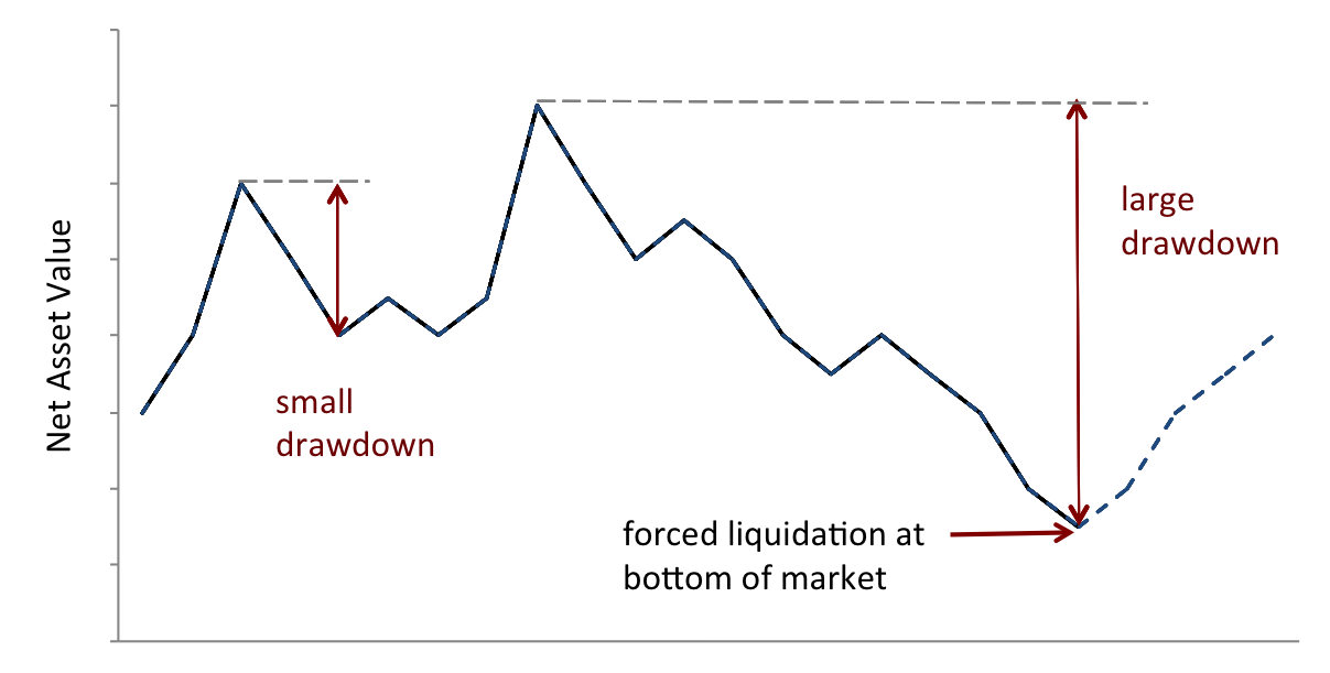
In the event of a large drawdown, common risk diagnostics, such as volatility, Value-at-Risk, and Expected Shortfall, at the end of the intended investment horizon are less significant. Indeed, within the universe of hedge funds and commodity trading advisors (CTAs), one of the most widely quoted measures of risk is maximum drawdown. The notion of drawdown has been extensively studied in the literature of applied probability theory, which we review in Section 1.1. However, a generally accepted mathematical methodology for forming expectations about future potential maximum drawdowns does not seem to exist in the investment management industry. Drawdown in the context of risk and deviation measures has failed to attract the same kind of applied research devoted to other more conventional risk measures.

Our purpose is to formulate a (i) mathematically sound and (ii) practically useful measure of drawdown risk. Our formalization of drawdown risk is achieved by modeling continuous-time cumulative returns within a time horizon $T\in(0,\infty)$ as a stochastic process $X$ representing return paths, to which a certain real-valued functional, the Conditional Expected Drawdown, is applied. Mathematically, the process $X$ is transformed to the random variable $\mu(X)$, representing the maximum drawdown within a finite path. At confidence level $\alpha\in[0,1]$, the Conditional Expected Drawdown CED_α is then defined to be the expected maximum drawdown given that some maximum drawdown threshold $\rm{DT}_{\alpha}$, the $\alpha$-quantile of the maximum drawdown distribution, is breached:

$$\rm{CED}_{\alpha}(X)=\mathbb{E}\left(\mu(X)\mid\mu(X)>\rm{DT}_{\alpha}\right).$$

In the context of quantitative risk measures, CED is a deviation measure in the sense of Rockafellar et al., (2002, 2006). In particular, this implies that CED is convex with respect to portfolio weights, which means that it promotes diversification and can be used in an optimizer. It is also homogenous of degree one, so that it supports linear risk attribution under Euler’s homogenous function theorem.

By focusing on the maximum of all drawdowns within a path of fixed length $T$, we address a highly relevant risk management concern affecting fund managers on a daily basis, who ask themselves: what is the expected maximum possible cumulative drop in net asset value within the investment horizon $T$? If this loss exceeds a certain threshold, the investor may be forced to liquidate. For a given investment horizon $T$, Conditional Expected Drawdown indicates this expected cumulative loss in excess of a threshold, and it can be measured for various confidence levels.

Because Conditional Expected Drawdown is defined as the tail mean of a distribution of maximum drawdowns, it is a downside risk metric perfectly analogous to Expected Shortfall, which is the tail mean of a return distribution. Hence, much of the theory and practice of Expected Shortfall carries over to Conditional Expected Drawdown.

We will show, however, that drawdown is inherently path dependent and accounts for serial correlation, whereas Expected Shortfall does not account for consecutive losses.

1.1. Literature Review

The notion of drawdown has been extensively studied in the literature of applied probability theory and in research addressing active portfolio management, which we review next. However, a generally accepted mathematical methodology for forming expectations about future potential maximum drawdowns does not seem to exist in either the investment management industry or the academic literature. Drawdown in the context of risk and deviation measures has hence failed to attract the same kind of applied research devoted to other more conventional risk measures. Our work hence complements the existing literature as it develops a mathematically sound and practically useful measure of drawdown risk.

The analytical assessment of drawdown magnitudes has been broadly studied in the literature of applied probability theory. To our knowledge, the earliest mathematical analysis of the maximum drawdown of a Brownian motion appeared in Taylor, (1975), and it was shortly afterwards generalized to time-homogenous diffusion processes by Lehoczky, (1977). Douady et al., (2000) and Magdon-Ismail et al., (2004) derive an infinite series expansion for a standard Brownian motion and a Brownian motion with a drift, respectively. The discussion of drawdown magnitude was extended to studying the frequency rate of drawdown for a Brownian motion in Landriault et al., (2015). Drawdowns of spectrally negative Lévy processes were analyzed in Mijatovic and Pistorius, (2012). The notion of drawup, which measures the maximum cumulative gain relative to a running minimum, has also been investigated probabilistically, particularly in terms of its relationship to drawdown; see for example Hadjiliadis and Vecer, (2006), Pospisil et al., (2009), and Zhang and Hadjiliadis, (2010).

Reduction of drawdown in active portfolio management has received considerable attention in mathematical finance research. Grossman and Zhou, (1993) considered an asset allocation problem subject to drawdown constraints; Cvitanic and Karatzas, (1995) extended the same optimization problem to the multi-variate framework; Chekhlov et al., (2003, 2005) developed a linear programming algorithm for a sample optimization of portfolio expected return subject to constraints on drawdown, which, in Krokhmal et al., (2003), was numerically compared to shortfall optimzation with applications to hedge funds in mind; Carr et al., (2011) introduced a new European style drawdown insurance contract and derivative-based drawdown hedging strategies; and most recently Cherney and Obloj, (2013), Sekine, (2013), Zhang et al., (2013) and Zhang, (2015) studied drawdown optimization and drawdown insurance under various stochastic modeling assumptions. Zabarankin et al., (2014) reformulated the necessary optimality conditions for a portfolio optimization problem with drawdown in the form of the Capital Asset Pricing Model (CAPM), which is used to derive a notion of drawdown beta. More measures of sensitivity to drawdown risk were introduced in terms of a class of drawdown Greeks in Pospisil and Vecer, (2010).

In the context of quantitative risk measurement, Chekhlov et al., (2003, 2005) develop a quantitative measure of drawdown risk called Conditional Drawdown at Risk (CDaR). Like CED, CDaR is a deviation measure (Rockafellar et al., (2002, 2006)). Unlike CED, however, CDaR focuses on all drawdowns rather than maximum drawdowns.

2. Measuring Drawdown Risk

We use the general setup of Cheridito et al., (2004) for the mathematical formalism of continuous-time path dependent risk. Continuous-time cumulative returns, or equivalently net asset value processes, are represented by essentially bounded càdlàg processes (in the given probability measure) that are adapted to the filtration of a filtered probability space. More formally, for a time horizon $T\in(0,\infty)$, let $(\Omega,\mathcal{F},\{\mathcal{F}_{t}\}_{t\in[0,T]},\mathbb{P})$ be a filtered probability space satisfying the usual assumptions, that is the probability space $(\Omega,\mathcal{F},\mathbb{P})$ is complete, $(\mathcal{F}_{t})$ is right-continuous, and $\mathcal{F}_{0}$ contains all null-sets of $\mathcal{F}$. For $p\in[1,\infty]$, $(\mathcal{F}_{t})$-adapted càdlàg processes lie in the Banach space

$$\mathcal{R}^{p}=\left\{X\colon[0,T]\times\Omega\to\mathbb{R}\mid X\hskip 5.0pt(\mathcal{F}_{t})\textrm{-adapted c\`{a}dl\`{a}g process },\|X\|_{\mathcal{R}^{p}}\right\},$$

which comes equipped with the norm

$$\|X\|_{\mathcal{R}^{p}}:=\|X^{*}\|_{p}$$

where $X^{*}=\sup_{t\in[0,T]}|X_{t}|$.

All equalities and inequalities between processes are understood throughout in the almost sure sense with respect to the probability measure $\mathbb{P}$. For example, for processes $X$ and $Y$, $X\leq Y$ means that for $\mathbb{P}$-almost all $\omega\in\Omega$, $X_{t}(\omega)\leq Y_{t}(\omega)$ for all $t$.

Definition 2.1 (Continuous-time path-dependent risk measure).

A continuous-time path-dependent risk measure is a real-valued function $\rho:\mathcal{R}^{\infty}\to\mathbb{R}$.

In practice, where one works in a discrete universe, this continuous-time setup is discretized by choosing the frequency of observations over the return horizon $T$. This adds a crucial parameter to the analysis, as higher frequency observations tend to yield larger drawdowns. Consider the May 2011 flash crash. When working at a daily frequency, one never sees the flash crash drawdown, no matter how long the investment horizon.

2.1. Maximum Drawdown

Definition 2.2 (Drawdown process).

For a horizon $T\in(0,\infty)$, the drawdown process $D^{(X)}:=\{D^{(X)}_{t}\}_{t\in[0,T]}$ corresponding to a stochastic process $X\in\mathcal{R}^{\infty}$ is defined by

$$D^{(X)}_{t}=M^{(X)}_{t}-X_{t}\ ,$$

where

$$M^{(X)}_{t}=\sup_{u\in[0,t]}X_{u}$$

is the running maximum of $X$ up to time $t$.

In practice, the use of the maximum drawdown as an indicator of risk is particularly popular in the universe of hedge funds and commodity trading advisors, where maximum drawdown adjusted performance measures, such as the Calmar ratio, the Sterling ratio and the Burke ratio, are frequently used.

Definition 2.3 (Maximum drawdown).

Within a fixed time horizon $T\in(0,\infty)$, the maximum drawdown of the stochastic process $X\in\mathcal{R}^{\infty}$ is the maximum drop from peak to trough of $X$ in $[0,T]$, and hence the largest amongst all drawdowns $D^{(X)}_{t}$:

$$\mu(X)=\sup_{t\in[0,T]}\{D^{(X)}_{t}\}.$$

Equivalently, maximum drawdown can be defined as the random variable obtained through the following transformation of the underlying stochastic process $X$:

$$\mu(X)=\sup_{t\in[0,T]}\sup_{s\in[t,T]}\left\{X_{s}-X_{t}\right\}\ .$$

Even though, in a given horizon, only a single maximum drawdown is realized along any given path, it is beneficial to consider the distribution from which the maximum drawdown is taken. By looking at the maximum drawdown distribution, one can form reasonable expectations about the size and frequency of maximum drawdowns for a given portfolio over a given investment horizon.

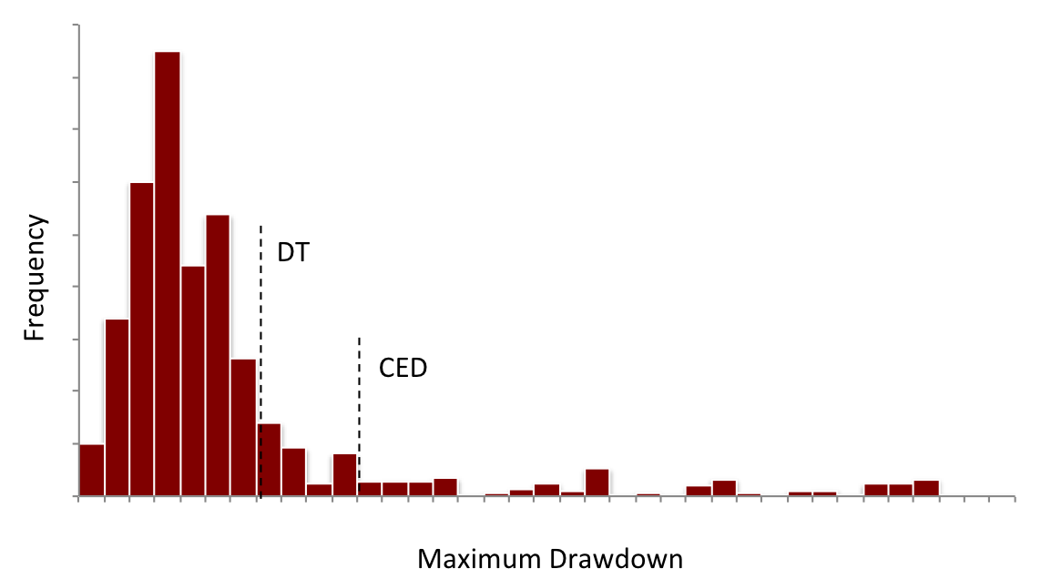
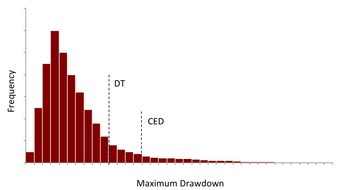
Figure 2.1 shows (A) the empirical maximum drawdown distribution (for paths of length 125 business days) of the daily S&P 500 time series over the period 1950 to 2013, and (B) the simulated distribution for an idealized Gaussian random variable. Both distributions are asymmetric, which implies that very large drawdowns occur less frequently than smaller ones. Using Monte Carlo simlations, Burghardt et al., (2003) show that maximum drawdown distributions are highly sensitive to the length of the track record (increases in the length of the track record shift the entire distribution to the right), mean return (for larger mean returns, the distribution is less skewed to the right, since large means tend to produce smaller maximum drawdowns, volatility of returns (higher volatility increases the likelihood of large drawdowns), and data frequency (a drawdown based on lower frequency data would ignore the flash crash).

The tail of the maximum drawdown distribution, from which the likelihood of a drawdown of a given magnitude can be distilled, is of particular interest in practice. Our drawdown risk metric, defined next, is a tail mean of the maximum drawdown distribution.

(a)

(b)

Figure 2.1. (A) Empirical distribution of the realized 6-month maximum drawdowns for the daily S&P 500 over the period 1 January 1950 to 31 December 2013, together with the 90% quantile (the drawdown threshold DT) and tail-mean (CED) of the distribution. (B) Distribution of 6-month maximum drawdowns for an idealized standard normally distributed random variable, together with the 90% quantile and tail-mean of the distribution.

2.2. Conditional Expected Drawdown

Our proposed drawdown risk metric, the Conditional Expected Drawdown (Definition 2.4), measures the average of worst case maximum drawdowns exceeding a quantile of the maximum drawdown distribution. Hence, it is analogous to the return-based Expected Shortfall (${\rm ES}$). Both ES and CED are given by the tail mean of an underlying distribution, namely that of the losses and maximum drawdowns, respectively.

Analogous to the return-based Value-at-Risk (VaR), we define, for confidence level $\alpha\in[0,1]$, the maximum drawdown threshold $\rm{DT}_{\alpha}$ to be a quantile of the maximum drawdown distribution:

$$\mathrm{DT}_{\alpha}\left(\mu(X)\right)=\inf\left\{m\mid\mathbb{P}\left(\mu(X)>m\right)\leq 1-\alpha\right\}$$

It is thus the smallest maximum drawdown $m$ for which the probability that the maximum drawdown $\mu(X)$ exceeds $m$ is at most $(1-\alpha)$. For example, the 95% maximum drawdown is both a worst case for drawdown in an ordinary period and a best case among extreme scenarios. It separates the 5% worst maximum drawdowns from the rest.

Definition 2.4 (Conditional Expected Drawdown).

At confidence level $\alpha\in[0,1]$, the Conditional Expected Drawdown CED${}_{\alpha}:\mathcal{R}^{\infty}\to\mathbb{R}$ is the function mapping $\mu(X)$ to the expected maximum drawdown given that the maximum drawdown threshold at $\alpha$ is breached. More formally,

$$\mathrm{CED}_{\alpha}\left(X\right)=\frac{1}{1-\alpha}\int_{\alpha}^{1}\rm{DT}_{\mathit{u}}\left(\mu(X)\right)d\mathit{u}.$$

If the distribution of $\mu(X)$ is continuous, then $\mathrm{CED}_{\alpha}$ is equivalent to the tail conditional expectation:

$$\rm{CED}_{\alpha}\left(X\right)=\mathbb{E}\left(\mu(X)\mid\mu(X)>\rm{DT}_{\alpha}\left(\mu(X)\right)\right).$$

In other words, CED is the tail mean (Acerbi and Tasche, 2002b ) over the maximum drawdown distribution, where for confidence level $\alpha\in(0,1)$, and assuming $\mathbb{E}[\mu(X)]<\infty$, the $\alpha$-tail mean of $\mu(X)$ is given by:

$$\mathrm{TM}_{\alpha}(\mu(X))=\frac{1}{1-\alpha}\int_{\alpha}^{1}\mathrm{DT}_{u}(\mu(X))d\mathit{u}\ .$$

3. Properties of Conditional Expected Drawdown

We derive theoretical properties of Conditional Expected Drawdown, most notably convexity and positive homogeneity, and prove that it is a generalized deviation measure, as developed by Rockafellar et al., (2002, 2006). Broadly speaking, deviation measures obey axioms taken from the properties of measures such as standard deviation and semideviation. We generalize these axioms to our path-dependent universe.

Definition 3.1 (Generalized Path-Dependent Deviation Measure).

A generalized path-dependent deviation measure is a path-dependent risk measure $\delta:\mathcal{R}^{\infty}\to\mathbb{R}$ satisfying the following axioms:

• Normalization: for all constant deterministic $C\in\mathcal{R}^{\infty}$, $\delta(C)=0$.

• Positivity: for all $X\in\mathcal{R}^{\infty}$, $\delta(X)\geq 0$.

• Shift invariance: for all $X\in\mathcal{R}^{\infty}$ and all constant deterministic $C\in\mathcal{R}^{\infty}$, $\delta(X+C)=\delta(X)$.

• Convexity: for all $X,Y\in\mathcal{R}^{\infty}$ and $\lambda\in[0,1]$, $\delta(\lambda+(1-\lambda)Y)\leq\lambda\delta(X)+(1-\lambda)\delta(Y)$.

• Positive degree-one homogeneity: for all $X\in\mathcal{R}^{\infty}$ and $\lambda>0$, $\delta(\lambda X)=\lambda\delta(X)$.

Any portfolio of zero value and, more generally, of constant deterministic value is not exposed to drawdown risk, and so for all constant deterministic $C\in\mathcal{R}^{\infty}$, we have $\mathrm{CED}_{\alpha}(C)=0$, and hence axiom (D0) is satisfied. Moreover, CED satisfies (D1) because maximum drawdown is by definition non-negative. The following Lemma proves the shift invariance property (D2), which essentially states that by (deterministically) shifting the path of the portfolio value up or down, the drawdown within that path remains unchanged.

Lemma 3.2.

For all $X\in\mathcal{R}^{\infty}$ and all constant almost surely $C\in\mathcal{R}^{\infty}$, $\mathrm{CED}_{\alpha}(X+C)=\mathrm{CED}_{\alpha}(X)$ (for all $\alpha\in(0,1)$).

Proof.

The drawdown process $D^{X}$ corresponding to $X$ is shift invariant, since for $t\in[0,T]$,

$$M_{t}^{(X+C)}=\sup_{u\in[0,t]}(X+C)_{u}=\sup_{u\in[0,t]}(X)_{u}+C=M_{t}^{(X)}+C\ .$$

It follows that $D^{(X+C)}=M^{(X+C)}-X-C=M^{(X)}+C-X-C=M^{(X)}-X=D^{(X)}$. Therefore,

$$\mu(X+C)=\sup_{t\in[0,T]}\left\{D_{t}^{(X+C)}\right\}=\sup_{t\in[0,T]}\left\{D_{t}^{(X)}\right\}=\mu(X)\ .$$

Hence, $\mathrm{CED}_{\alpha}(X+C)=\mathrm{CED}_{\alpha}(X)$.
∎

We next focus on the properties of convexity (D3) and positive homogeneity (D4) of generalized deviation measures.

3.1. Convexity of CED

According to Föllmer and Schied, (2002, 2010, 2011), the essence of diversification is encapsulated in the convexity axiom. Suppose we have two processes $X$ and $Y$ representing cumuative returns to two portfolios. Rather than investing fully in one of the two portfolios, an investor could diversify by allocating a fraction $\lambda\in[0,1]$ of his capital to, say, $X$, and the remainder $1-\lambda$ to $Y$. Under a convex risk measure, this diversification cannot increase risk.

Proposition 3.3 (Convexity of CED).

Conditional Expected Drawdown is convex with respect to portfolio weights: for all $X,Y\in\mathcal{R}^{\infty}$, $\lambda\in[0,1]$, and confidence level $\alpha\in(0,1)$, $\mathrm{CED}_{\alpha}(\lambda+(1-\lambda)Y)\leq\lambda\mathrm{CED}_{\alpha}(X)+(1-\lambda)\mathrm{CED}_{\alpha}(Y)$.

Proof.

For $\lambda\in[0,1]$, we have $M^{(\lambda X+(1-\lambda)Y)}\leq\lambda M^{(X)}+(1-\lambda)M^{(Y)}$ by properties of the supremum, and therefore

$$D^{(\lambda X+(1-\lambda)Y)} = M^{(\lambda X+(1-\lambda)Y)}-\lambda X-(1+\lambda)Y$$

$$\leq \lambda M^{(X)}+(1-\lambda)M^{(Y)}-\lambda X-(1+\lambda)Y$$

$$= \lambda D^{(X)}+(1-\lambda)D^{(Y)}$$

Assuming that the distributions of $\mu(X)$ and $\mu(Y)$ are continuous, and because $\mu(X)$ is defined as the supremum within the drawdown path $D$, we have $\mu(\lambda X+(1-\lambda)Y)\leq\lambda\mu(X)+(1-\lambda)\mu(Y)$. Finally, since the tail mean functional $\mathrm{TM}$ is subadditive and positive homogenous independent of the underlying distribution (see Acerbi and Tasche, 2002a ; Acerbi and Tasche, 2002b ), and also monotonically non-decreasing, its composite with $\mu$ is also convex, and so $\mathrm{CED}_{\alpha}(\lambda+(1-\lambda)Y)\leq\lambda\mathrm{CED}_{\alpha}(X)+(1-\lambda)\mathrm{CED}_{\alpha}(Y)$. ∎

Remark 3.4 (Drawdown risk optimization).

Convexity of CED implies that one can, in theory, allocate assets to trade off CED risk against portfolio return. There are three crucial ingredients for carrying out any optimization in practice. Convexity of the objective function to be minimized ensures that the minimum, if it exists, is a global one. The second ingredient is the feasibility and efficiency of the optimization algorithm. Seminal work of Rockafellar and Uryasev, (2000, 2002), who developed an efficient linear programming (LP) algorithm for minimizing the tail mean of a distribution of returns, and of Chekhlov et al., (2003, 2005), who incorporated drawdown into the LP formulation, can in theory be used to minimize the tail mean of a maximum drawdown distribution. The third ingredient, which allows us to move beyond theory, is an empirically sound estimate of risk. Further empirical exploration of the properties of CED and the study of its impact on quantitative portfolio construction, are necessary and beyond the scope of this article.

3.2. Positive Homogeneity of CED

Degree-one positive homogenous risk measures are characterized by Euler’s homogenous function theorem, and hence play a prominent role in portfolio risk analysis. More precisely, for a portfolio $P=\sum_{i}w_{i}X_{i}$ in $\mathcal{R}^{\infty}$, a risk measure $\rho:\mathcal{R}^{\infty}\to\mathbb{R}$ is postive homogenous of degree one if and only if $\sum_{i}w_{i}\left(\partial\rho(P)\right)/(\partial w_{i})=\rho(P)$. The risk $\rho(P)$ of the portfolio $P=\sum_{i}w_{i}X_{i}$ can therefore be linearly attributed along its factors $X_{i}$.

Proposition 3.5 (Positive homogeneity of CED).

Conditional Expected Drawdown is degree-one positive homogenous with respect to portfolio weights: for all $X\in\mathcal{R}^{\infty}$, $\lambda>0$ and confidence level $\alpha\in(0,1)$, $\mathrm{CED}_{\alpha}(\lambda X)=\lambda\mathrm{CED}_{\alpha}(X)$.

Proof.

For $\lambda>0$, we have for $t\in[0,T]$, $M_{t}^{(\lambda X)}=\sup_{u\in[0,t]}(\lambda X)_{u}=\lambda\sup_{u\in[0,t]}(X)_{u}=\lambda M_{t}^{(X)}$, and therefore $D^{(\lambda X)}=\lambda M^{(X)}-\lambda X=\lambda D^{(X)}$. Because $\mu(X)$ is defined as the supremum within the drawdown path $D$, we have $\mu(\lambda X)=\lambda\mu(X)$. Finally, positive homogeneity of the tail mean functional yields the result.
∎

4. Drawdown Risk Attribution

With the theoretical framework of drawdown risk measurement in place, the next step is to understand how Conditional Expected Drawdown can be integrated in the investment process. We show how to systematically analyze the sources of drawdown risk within a portfolio and how these sources interact. In practice, investors may be interested in attributing risk to individual securities, asset classes, sectors, industries, currencies, or style factors of a particular risk model. In what follows, we assume a generic such risk factor model.

Fix an investment period and let $F_{i}$ denote the return of factor $i$ over this period ($1\leq i\leq n$). Then the portfolio return over the period is given by the sum

$$P=\sum_{i=1}^{n}w_{i}F_{i}\ ,$$

where $w_{i}$ is the portfolio exposure to factor $i$ and the summand representing idiosyncratic risk is not included for simplicity. Because portfolio risk is not a weighted sum of source risks, there is no direct analog to this decomposition for risk measures. However, there is a parallel in terms of marginal risk contributions (MRC), which are interpreted as a position’s percent contribution to overall portfolio risk. They provide a mathematically and economically sound way of decomposing risk into additive subcomponents.

For a risk measure $\rho$, the marginal contribution to risk of a factor is the approximate change in overall portfolio risk when increasing the factor exposure by a small amount, while keeping all other exposures fixed. Formally, marginal risk contributions can be defined for any differentiable risk measure $\rho$.

Definition 4.1.

For a factor $F_{i}$ in the portfolio $P=\sum_{i}w_{i}F_{i}$, its marginal risk contribution $\mathrm{MRC}_{i}$ is the derivative of the underlying risk measure $\rho$ along its exposure $w_{i}$:

$$\mathrm{MRC}_{i}^{\rho}(P)=\frac{\partial\rho(P)}{\partial w_{i}}.$$

If $\rho$ is homogenous of degree one, the overall portfolio risk can be decomposed using Euler’s homogoneous function theorem as follows:

$$\sum_{i}w_{i}\mathrm{MRC}_{i}^{\rho}(P)=\sum_{i}{\rm RC}_{i}^{\rho}(P)=\rho(P),$$

where ${\rm RC}_{i}^{\rho}(P)=w_{i}\mathrm{MRC}_{i}^{\rho}(P)$ is the $i$-th total risk contribution to $\rho$. Finally, fractional risk contributions

$$\mathrm{FRC}_{i}^{\rho}(P)=\frac{{\rm RC}_{i}^{\rho}(P)}{\rho(P)}$$

denote the fractional contribution of the $i$-th factor to portfolio risk.

Risk contributions implicitly define a notion of correlation that is general enough to be defined for any risk measure. The generalized risk-based correlation $\rm Corr_{i}^{\rho}$ for a generic risk measure $\rho:\mathcal{M}\to\mathbb{R}$ between the portfolio and the $i$th asset $X_{i}$ is defined by:

$$\rm Corr_{i}^{\rho}=\frac{\mathrm{MRC}_{i}^{\rho}(P)}{\rho(X_{i})}.$$

Generalized correlations are monotonically decreasing in position weight. Factoring out the $i$th marginal risk $\rho(X_{i})$ from the $i$th risk contribution ${\rm RC}_{i}(P)$, we obtain the generalized form of the “X-Sigma-Rho” decomposition of Menchero and Poduri, (2008):

$${\rm RC}^{\rho}_{i}(P)=w_{i}\rho(X_{i})\frac{\mathrm{MRC}^{\rho}_{i}(P)}{\rho(X_{i})}=w_{i}\rho(X_{i})\rm Corr^{\rho}_{i}\quad.$$

We refer the reader Goldberg et al., (2010) for a more detailed development of generalized correlations.

4.1. Drawdown Risk Contributions

Menchero and Poduri, (2008) and Goldberg et al., (2010) developed a standard toolkit for analyzing portfolio risk using a framework centered around marginal risk contributions. By integrating drawdown risk into this framework, investors can estimate how a trade would impact the overall drawdown risk of the portfolio. Because Conditional Expected Drawdown is positive homogenous, the individual factor contributions to drawdown risk add up to the overall drawdown risk within a path $P\in\mathcal{R}^{\infty}$ of returns to a portfolio with values at time $t\leq T$ given by $P_{t}=\sum_{i}w_{i}F_{i,t}$:

(4.1) $$\mathrm{CED}_{\alpha}(P)=\sum_{i}{w_{i}{\mathrm{MRC}}_{i}^{\mathrm{CED}_{\alpha}}(P)},\quad\alpha\in[0,1].$$

Recall that a marginal risk contribution is a partial derivative, and so practitioners can implement Formula 4.1 using numerical differentiation. However, this tends to introduce noise. We next show that an individual marginal contribution to drawdown risk can be expressed as an integral, and this reduces noise, since integration is a smoothing operator. Indeed, the individual marginal contribution ${\mathrm{MRC}}_{i}^{\mathrm{CED}_{\alpha}}$ of the $i$-th factor to overall portfolio drawdown risk $\mathrm{CED}_{\alpha}(P)$ is given by the expected drop of the $i$-th factor in the interval $[s^{*},t^{*}]\subset[0,T]$ where the overall portfolio maximum drawdown $\mu(P)$ occurs, given that the maximum drawdown of the overall portfolio exceeds the drawdown threshold. This definition is analogous to the marginal contribution to shortfall, and we formalize it next.

Proposition 4.2.

Marginal contributions to drawdown risk are given by:

(4.2) $$\mathrm{MRC}_{i}^{\mathrm{CED}_{\alpha}}(P)=\mathbb{E}\left[\left(F_{i,t^{*}}-F_{i,s^{*}}\right)\mid\mu(P)>\mathrm{DT}_{\alpha}(P)\right],$$

where $\mathrm{CED}_{\alpha}(P)$ is the overall portfolio CED, $\mu(P)$ is the maximum drawown random variable, $\rm{DT}_{\alpha}(P)$ is the portfolio maximum drawdown threshold at $\alpha$, and $s^{*}<t^{*}\leq T$ are random times such that:

$$\mu(P)=P_{t^{*}}-P_{s^{*}},$$

and we assume that the maximum drawdown of $P=\sum_{i}w_{i}F_{i}$ is strictly positive.

Proof.

We use the results of Tasche, (2002), Goldberg et al., (2010) and McNeil et al., (2005), who show that the $i$-th marginal contribution to Expected Shortfall ${\rm ES}_{\alpha}$ at confidence level $\alpha\in(0,1)$ of a random variable $L=\sum_{i}w_{i}Y_{i}$ representing portfolio loss is given by

(4.3) $$\mathrm{MRC}_{i}^{{\rm ES}_{\alpha}}(L)=\mathbb{E}\left[Y_{i}\mid L>{\rm Var}_{\alpha}(L)\right],$$

where ${\rm Var}_{\alpha}(L)$ denotes the Value-at-Risk of $L$ at $\alpha$, that is the $\alpha$-quantile of the loss distribution $L$.

We derive an analog to Formula 4.3. Assuming that the maximum drawdown of $P=\sum_{i}w_{i}F_{i}$ is strictly positive, let

$$\mu(P)=P_{t^{*}}-P_{s^{*}}$$

for some $s^{*}<t^{*}\leq T$. Then the $i$-th marginal contribution $\mathrm{MRC}_{i}^{\mathrm{CED}_{\alpha}}(P)$ to overall portfolio drawdown risk $\mathrm{CED}_{\alpha}(P)$ is given by

(4.4) $$\mathrm{MRC}_{i}^{\mathrm{CED}_{\alpha}}(P) = \frac{\partial}{\partial w_{i}}\left(\mathrm{TM}_{\alpha}\left(\mu(P)\right)\right)$$

$$= \frac{\partial}{\partial w_{i}}\mathbb{E}\left[\mu(P)\mid\mu(P)>\mathrm{DT}_{\alpha}(P)\right]$$

$$= \frac{\partial}{\partial w_{i}}\mathbb{E}\left[(P_{t^{*}}-P_{s^{*}})\mid\mu(P)>\mathrm{DT}_{\alpha}(P)\right]$$

$$= \frac{\partial}{\partial w_{i}}\mathbb{E}\left[\left(\sum_{i=1}^{n}w_{i}F_{i,t^{*}}-\sum_{i=1}^{n}w_{i}F_{i,s^{*}}\right)\mid\mu(P)>\mathrm{DT}_{\alpha}(P)\right]$$

$$= \frac{\partial}{\partial w_{i}}\mathbb{E}\left[\sum_{i=1}^{n}w_{i}\left(F_{i,t^{*}}-F_{i,s^{*}}\right)\mid\mu(P)>\mathrm{DT}_{\alpha}(P)\right]$$

$$= \frac{\partial}{\partial w_{i}}\left(\sum_{i=1}^{n}w_{i}\mathbb{E}\left[\left(F_{i,t^{*}}-F_{i,s^{*}}\right)\mid\mu(P)>\mathrm{DT}_{\alpha}(P)\right]\right)$$

Using the fact that the partial derivative with respect to a quantile is zero, as discussed by Bertsimas et al., (2004), Formula 4.4 simplifies to:

$$\mathrm{MRC}_{i}^{\mathrm{CED}_{\alpha}}(P)=\mathbb{E}\left[\left(F_{i,t^{*}}-F_{i,s^{*}}\right)\mid\mu(P)>\mathrm{DT}_{\alpha}(P)\right].$$

Finally, note that the variables $s^{*}$ and $t^{*}$ are stochastic. This means that in a Monte Carlo simulation of a discretized version of this problem, they will take on a different value scenario by scenario. ∎

5. Empirical Analysis of Drawdown Risk

We analyze historical values of Conditional Expected Drawdown based on daily data for two asset classes: US Equity and US Government Bonds. The US Government Bond Index we use includes fixed income securities issued by the US Treasury (excluding inflation-protected bonds) and US government agencies and instrumentalities, as well as corporate or dollar-denominated foreign debt guaranteed by the US government, with maturities greater than 10 years. These include government agencies such as the Federal National Mortgage Association (Fannie Mae) and the Federal Home Loan Mortgage Corporation (Freddie Mac) without an explicit guarantee. In comparison to US Treasury Bond Indices, US Government Bond Indices were highly volatile and correlated with US Equities during the financial crisis of 2008. The effect of this will be seen in our empirical analysis. Summary risk statistics for the two asset classes and three fixed-mix portfolios are shown in Table 5.1.

5.1. Time-varying Drawdown Risk Concentrations

	Volatility	ES0.9	CED0.9 (6M-paths)	CED0.9 (1Y-paths)	CED0.9 (5Y-paths)
US Equity	18.35%	2.19%	47%	51%	57%
US Bonds	5.43%	0.49%	29%	32%	35%
50/50	9.53%	1.30%	31%	32%	35%
60/40	11.12%	1.35%	33%	35%	38%
70/30	12.92%	1.40%	36%	40%	44%

Table 5.1. Summary statistics for daily US Equity and US Bond Indices and three fixed-mix portfolios over the period 1 January 1982 to 31 December 2013. Expected Shortfall and Conditional Expected Drawdown are calculated at the 90% confidence level. Three drawdown risk metrics are calculated by considering the maximum drawdown within return paths of different fixed lengths (6 months, 1 year and 5 years).

Using the definition of marginal contributions to Conditional Expected Drawdown (derived in Proposition 4.2), we look at the time varying contributions to CED. Figure 5.1 displays the daily 6-month rolling fractional contributions to drawdown risk $\mathrm{CED}_{0.9}$ (at the 90% threshold of the 6-month maximum drawdown distribution) of the two asset classes (US Equity and US Bonds) in the balanced 60/40 allocation. Between 1982 and 2008, and between 2012 and 2013, the contributions of US Equity to overall drawdown risk fluctuated between 80% and 100%. Note that this period includes two of the three turbulent market regimes that occurred during this 30-year window, namely the 1987 stock market crash and the burst of the internet bubble in the early millennium. During the credit crisis of 2008, however, we see, unexpectedly, that bonds contributed almost as much as equities to portfolio drawdown risk.

Figure 5.1. Daily 6-month rolling Fractional Risk Contributions (FRC) along the 90% Conditional Expected Drawdown (CED) of US Equity and US Bonds to the balanced 60/40 portfolio. Also displayed is the daily VIX series over the period 1982 – 2013, with the right-hand axis indicating its level.

Figure 5.2. Decomposition of the individual contributions to drawdown risk ${\rm RC}^{\mathrm{CED}}_{i}(P)=w_{i}\mathrm{CED}(X_{i})\rm Corr^{\mathrm{CED}}_{i}$ for the 60/40 allocation to US Equity and US Bonds over the period 1982 – 2013. The top two panels show the daily 6-month rolling standalone 90% Conditional Expected Drawdown (CED) of the two asset classes, while the bottom two panels show the daily 6-month rolling generalized correlations of the individual assets along CED.

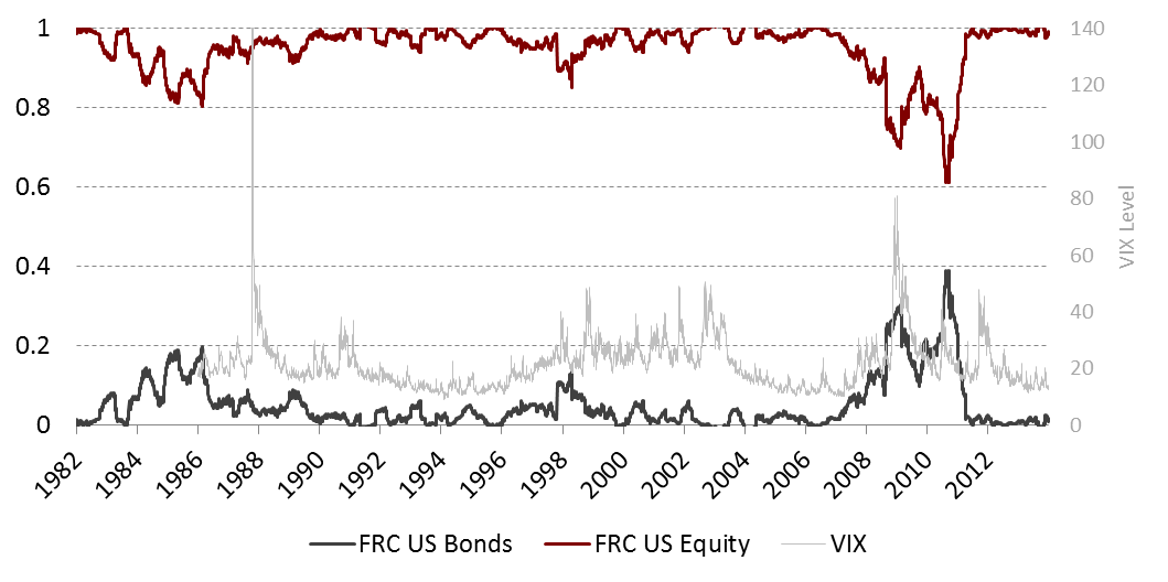
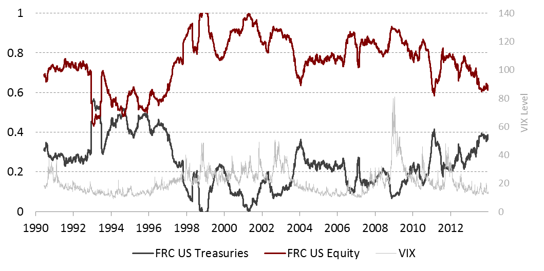
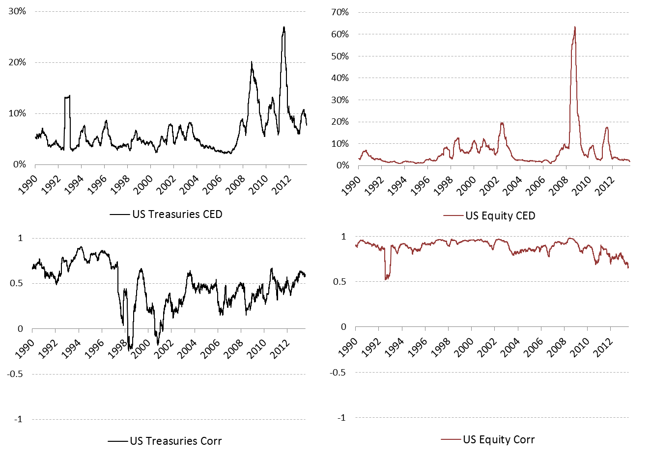
Our analysis shows little connection between market turbulence and drawdown risk concentration in the 60/40 fixed mix of US Equity and US Bonds. Notably, the most equitable attribution of drawdown risk occurred during the 2008 financial crisis. This can be explained by the inclusion of bonds issued by Fannie Mae and Freddie Mac in the US Government Bond Index. In calm regimes, these Agency Bonds tended to be correlated with US Treasury bonds, but during the financial crisis, Agency Bonds were more correlated with US Equity. For comparison, we provide the same analysis when the underlying Bond Index used is the US Treasury Bond Index (see Figures B.1 and B.2 in Appendix B). In this case, as one would expect, the least equitable attribution of drawdown risk occurred during turbulent market periods.

To understand the sources of the risk contributions, particularly during the credit crisis of 2008 where the concentrations of US Equity and US Government Bonds approached parity, we carry out the “X-Sigma-Rho” decomposition of Menchero and Poduri, (2008). Recall from Section 4 that risk contribution is proportional to the product of standalone risk and generalized correlation. In the case of Conditional Expected Drawdown, this means that:

$${\rm RC}^{\mathrm{CED}}_{i}(P)=w_{i}\mathrm{CED}(X_{i})\rm Corr^{\mathrm{CED}}_{i}.$$

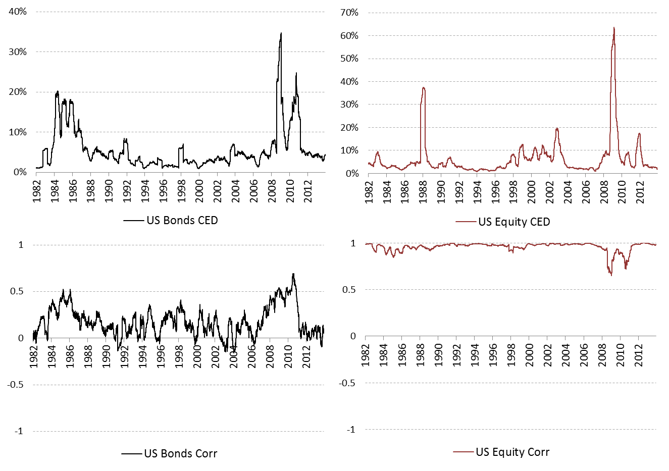
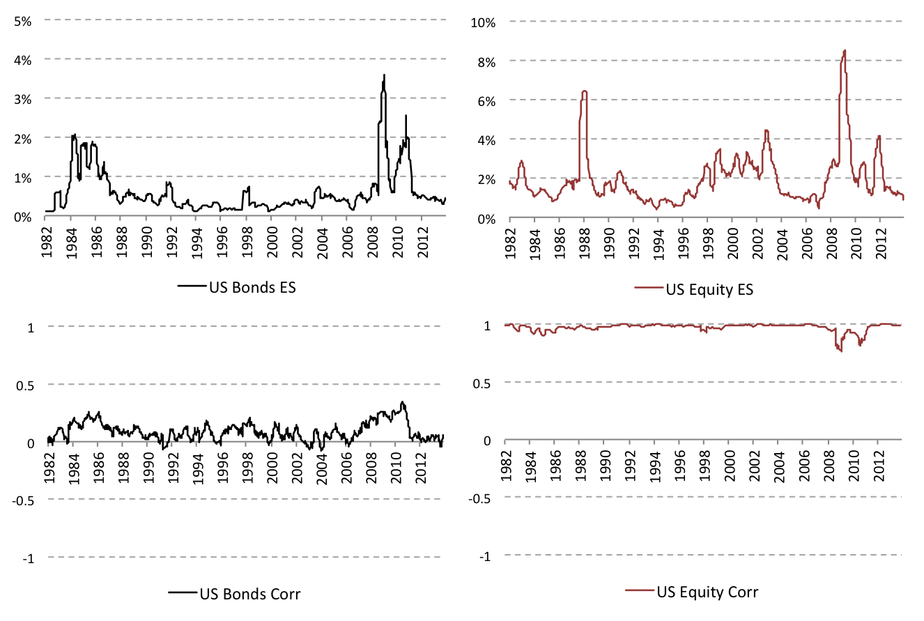
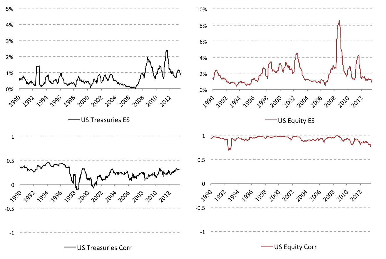
Because we are working with a fixed-mix portfolio, the exposures $w_{i}$ are constant: 0.6 and 0.4 for US Equity and US Bonds, respectively. This means that the time-varying risk contributions of Figure 5.1 depend on the time-varying drawdowns ($\mathrm{CED}(X_{i})$) and correlations ($\rm Corr^{\mathrm{CED}}_{i}$). Figure 5.2 displays these for each of the two assets in our 60/40 portfolio. Observe that during the 2008 financial crisis, both the drawdown risk contribution of US Bonds and its generalized correlation were elevated relative to the subsequent period. On the other hand, the generalized correlation of US Equity during the 2008 crisis decreased. The combination of these effects may have driven the changes in the drawdown contributions of US Bonds and US Equity during the 2008 crisis.

In Section 5.2, we give a statistical analysis that supports the economic explanation of the increased CED values for US Government Bonds. In practice, investors can efficiently control such regime-dependent fluctuations in drawdown risk concentrations since Conditional Expected Drawdown is a convex risk measure; that is both the return path and the drawdown path are convex with respect to asset weights. Hence, they are convex functions of factors that are linear combinations of asset weights. This implies that reducing the portfolio exposure to an asset or factor in a linear factor model decreases its marginal contribution to overall portfolio drawdown.

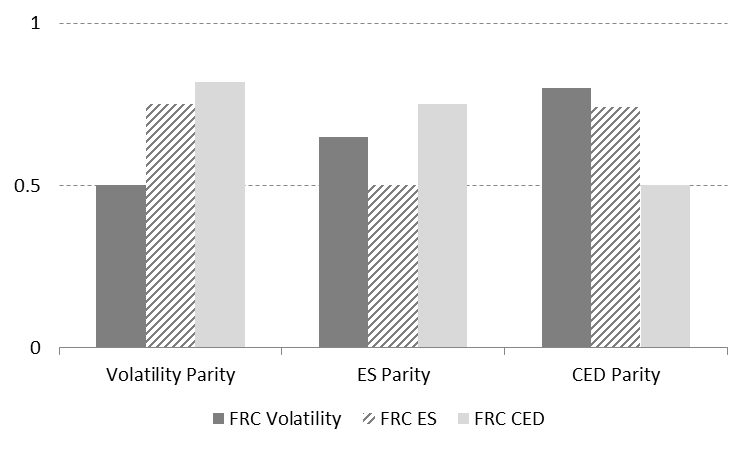
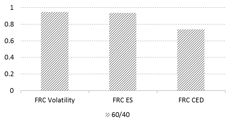
It is possible for a portfolio to have equal risk contributions with respect to one measure while harboring a substantial concentration with respect to another. Figure 5.3 illustrates such a case. Four portfolios are constructed to be maximally diversified along the following risk measures: volatility, Expected Shortfall, and Conditional Expected Drawdown. The underlying asset classes are US Equity and US Government Bonds as before from 1982 to 2013. We refer to these as being in parity with respect to the underlying risk measure. The confidence level for both ES and CED is fixed at 90%. Figure 5.3 shows fractional risk contribution of the equity component to each of three risk measures in three types of risk parity portfolios. Concentrations in terms of drawdown risk, in particular, are revealed. For instance, even though the ES Parity portfolio, which has equal contributions to Expected Shortfall, is constructed to minimize downside risk concentrations, it turns out to have 75% of its drawdown risk concentrated in US Equity.

Figure 5.3. Fractional Risk Contributions (FRC) of US Equity measured along three different risk measures (volatility, 90% Expected Shortfall and 90% Conditional Expected Drawdown) for the following two-asset portfolios consisting of US Equity and US Bonds over the period 1982–2013: Volatility Parity, ES Parity and CED Parity. Each parity portfolio is constructed to have equal risk contributions along its eponymous risk measure.

5.2. Drawdown Risk and Serial Correlation

One advantage of looking at maximum drawdown distributions rather than return distributions, and thus Conditional Expected Drawdown rather than Expected Shortfall, lies in the fact that drawdown is inherently path dependent. In other words, drawdown measures the degree to which losses are sustained, as small but persistent cumulative losses may still lead to large drops in portfolio net asset value, and hence may force liquidation. On the other hand, volatility and Expected Shortfall fail to distinguish between intermittent and consecutive losses. We show that, to a greater degree than these two risk measures, Conditional Expected Drawdown captures temporal dependence. Moreover, the effect of serial correlation on drawdown risk can be seen in the drawdown risk contributions.

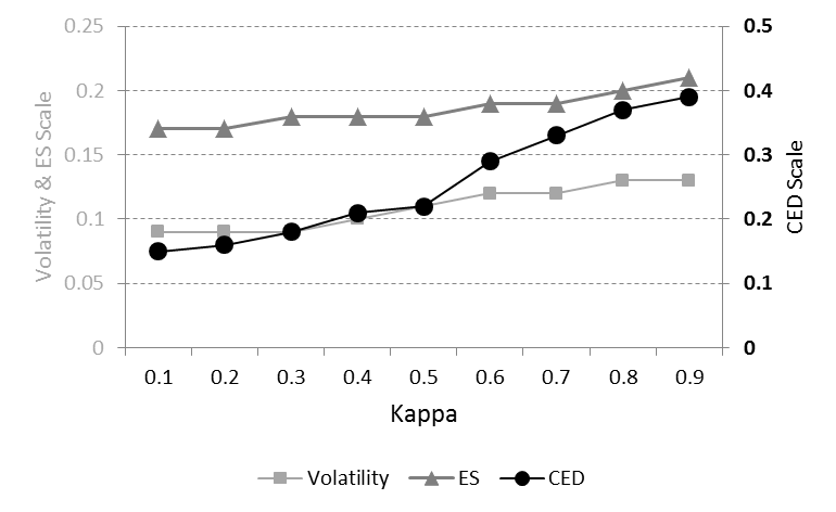
An increase in serial correlation increases drawdown risk. To see how temporal dependence affects risk measures, we use Monte Carlo simulation to generate an autoregressive AR(1) model:

$$r_{t}=\kappa r_{t-1}+\epsilon_{t},$$

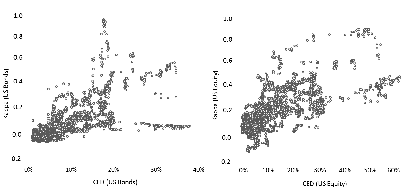
with varying values for the autoregressive parameter $\kappa$ (while $\epsilon$ is Gaussian with variance 0.01), and calculate volatility, Expected Shortfall, and Conditional Expected Drawdown of each simulated autoregressive time series. Figure 5.4 displays the results. All three risk measures were affected by the increase in the value of the autoregressive parameter, but the increase is steepest by far for CED. We next use maximum likelihood to fit the AR(1) model to the daily time series of US Equity and US Government Bonds on a 6-month rolling basis to obtain time series of estimated $\kappa$ values for each asset. The correlations of the time series of $\kappa$ with the time series of 6-month rolling volatility, Expected Shortfall, and Conditional Expected Drawdown are shown in Table 5.2. The correlations are substantially higher for US Equity across all three risk measures. Note that for both asset classes, the correlation with the autoregressive parameter is highest for CED. Figure 5.5 contains the scatter plots of estimated $\kappa$ parameters for US Equity and US Bonds against their CED.

Figure 5.4. Volatility, 90% Expected Shortfall (ES), and 90% Conditional Expected Drawdown (CED) of a Monte Carlo simulated AR(1) model (with 10,000 data points) for varying values of the autoregressive parameter $\kappa$.

	Volatility	ES0.9	CED0.9
US Equity	0.47	0.52	0.75
US Bonds	0.32	0.39	0.69

Table 5.2. For the daily time series of each of US Equity and US Government Bonds, correlations of estimates of the autoregressive parameter $\kappa$ in an AR(1) model with the values of the three risk measures (volatility, 90% Expected Shortfall and 90% Conditional Expected Drawdown) estimated over the entire period (1982–2013).

Figure 5.5. For each of US Equity and US Government Bonds, scatter plots of the daily time series of 6-month rolling estimates of the autoregressive parameter $\kappa$ with the 6-month rolling estimates of 90% Conditional Expected Drawdown.

An increase in serial correlation increases drawdown risk concentrations. We now show how temporal dependence is manifest in the drawdown risk contributions. Figure 6(a) shows the fractional risk contributions over the entire period 1982–2013 of US Equity to the balanced 60/40 portfolio for three risk measures, volatility, ES, and CED, based on daily data. The fractional contributions of US Equity to volatility and ES were large (over 90%) and close in magnitude. For CED, however, the concentration was less pronounced, which means that the contribution of US Bonds to drawdown risk exceeded its contribution to volatility and shortfall risk. A candidate explanation is temporal dependence: while bonds systematically have lower volatility and shortfall risk than do equities, they do occasionally suffer from extended periods of consecutive losses.

To test this hypothesis, we simulate the returns $r_{E}$ and $r_{B}$ to two assets $E$ and $B$ representing equities and bonds, respectively, with an autoregressive AR(1) model:

$$r_{E,t}=\kappa_{E}r_{E,t-1}+\epsilon_{E,t},$$

and

$$r_{B,t}=\kappa_{B}r_{B,t-1}+\epsilon_{B,t},$$

and we construct a simulated 60/40 fixed-mix portfolio. The AR(1) model parameters are obtained by calibrating to daily time series of US Equity and US Bonds. The estimated autoregressive parameters are $\kappa_{E}=0.43$ and $\kappa_{B}=0.35$. We assume the $\epsilon$ variable is Gaussian, with volatility of 18.4% for asset E (based on the volatility of US Equity) and 5.5% for asset B, (based on the volatility of US Bonds). From the simulated data, we fit AR(1) models and their fractional contributions to volatility, ES and CED. When using only the residuals, we obtain statistically equal risk contributions since the innovations are Gaussian. However, without removing the autoregressive component, contributions to CED once again differ from contributions to volatility and ES. Figure 6(b) displays the corresponding fractional contributions of the more volatile asset class, $E$, to the three risk measures. Note that the two panels in Figure 5.6 are visually indistinguishable even though one is based on historical data, whereas the other is simulated.

(a)

(b)

Figure 5.6. (A) Fractional contributions over the entire period 1982–2013 of the US Equity asset to volatility, 90% Expected Shortfall and 90% Conditional Expected Drawdown in the 60/40 portfolio, based on daily data. (B) Fractional contributions of the simulated high-volatility AR(1) asset to volatility, 90% Expected Shortfall and 90% Conditional Expected Drawdown in the 60/40 portfolio.

6. Drawdown: From Practice to Theory and Back Again

Financial practitioners rely on maximum drawdown as an indicator of investment risk. However, due to its inherent path dependency, maximum drawdown has tended to fall outside of probabilistic treatments of investment risk, which focus on return and loss distributions at fixed horizons. As a result, maximum drawdown has been excluded from standard portfolio analysis toolkits that attribute risk to factors or asset classes, and that use risk forecasts as counterweights to expected return in portfolio construction routines.

In this article, we develop a new probabilistic measure of drawdown risk, Conditional Expected Drawdown (CED), which is the tail-mean of a drawdown distribution at a fixed horizon. Since CED is perfectly analogous to the familiar return-based risk measure, Expected Shortfall (ES), CED is easy for practitioners to interpret and it enjoys desirable theoretical properties of tail-means such as positive degree-one homogeneity and convexity. Thus, the development of a consistent theory for drawdown facilitates an extension of its current practical applications.

The path dependency of Conditional Expected Drawdown makes it more sensitive to serial correlation than Expected Shortfall or volatility. We demonstrate this using a simulated AR(1) model. All else equal, CED increases much more rapidly as a function of the autoregressive parameter $\kappa$ than do Expected Shortfall or volatility. In an empirical study, we find relatively high correlations between serial correlation and estimated CED (.75 for US Equity, .69 for US Bonds) compared to Expected Shortfall (.52 for US Equity, .39 for US Bonds) and volatility (.47 for US Equity, .32 for US Bonds).

Since it is positive degree-one homogenous, CED (like ES and volatility) can be decomposed into a sum of risk contributions, and the relative sensitivity of CED to serial correlation is manifest in risk concentrations. In an empirical study of a balanced 60/40 portfolio of US Equity and US Bonds over the period 1982–2013, US Equity accounted for roughly 75% of CED, but more than 90% of ES and volatility. A plausible explanation is the relatively high level of serial correlation in US Bonds. We support this hypothesis with another simulation: we replicate the empirically observed concentrations of CED, ES and volatility using a simulated 60/40 balanced portfolio based on AR(1) models calibrate to US Equity and US Bonds over the study period.

Since CED is convex, it can serve as a counterweight to expected return in a quantitative optimization. Exploiting the parallels between Expected Shortfall as a tail-mean of a return distribution and Conditional Expected Drawdown as a tail-mean of a drawdown distribution, one can in theory use the linear programming algorithm developed by Rockafellar and Uryasev, (2000, 2002).

This article lays the foundation needed to incorporate Conditional Expected Drawdown in the investment process. Further empirical exploration of the properties of CED, research into the incremental information it adds beyond what is in return-based risk measures, and the study of its impact on quantitative portfolio construction, are the next steps.

Appendix A Data and Estimation Methodologies

A.1. Data

The data were obtained from the Global Financial Data database. We took the daily time series for the S&P 500 Index and the USA 10-year Government Bond Total Return Index.

A.2. Portfolio Construction

Rather than provide thorough realistic empirical analyses of portfolio risk and return, our goal behind the simulated portfolios is to illustrate this article’s theoretical development in relation to drawdown risk. For simplicity, we therefore do not account for transaction costs or market frictions in all hypothetical portfolios constructed throughout this study. Moreover, we assume that all portfolios are fully invested and long only.

Fixed-mix portfolios. In the fixed-mix portfolios, rebalancing to the fixed weights is done on a monthly basis. When comparing to other popular rebalancing schemes (quarterly, bi-annually and yearly), similar results were obtained.

Risk parity portfolios. In risk parity strategies, assets are weighted so their ex post risk contributions are equal. As mentioned in Section 5, parity portfolios are not restricted to volatility only, but can be constructed along other risk measures, such as Expected Shortfall and Conditional Expected Drawdown. Asset weights in the strategies depend on estimates of the underlying risk measures (see Section A.3), which are calculated using a 3-year rolling window of trailing returns. Varying the estimation methodology by changing the length of the rolling window or the weighting scheme applied to the returns within this window did not alter our results substantially. Similar to the fixed-mix portfolios, risk parity portfolios are rebalanced monthly, with other rebelancing schemes yielding similar results.

A.3. Risk Estimation

Volatility. Portfolio volatility is calculated as the annualized standard deviation of the daily time series over the entire period under consideration. To obtain the volatility risk contributions for a $n$-asset portfolio $P=\sum_{i}w_{i}X_{i}$, note that the $i$-th total contribution ${\rm RC}_{i}^{\sigma}$ to portfolio volatility

$$\sigma(P)=\sum_{i}w_{i}^{2}\sigma_{i}^{2}+\sum_{i}\sum_{j\neq i}w_{i}w_{j}\sigma_{i,j}$$

is

$${\rm RC}_{i}^{\sigma}=w_{i}^{2}\sigma_{i}^{2}+\sum_{j\neq i}w_{i}w_{j}\sigma_{i,j},$$

where $\sigma_{i}^{2}$ is the variance of $X_{i}$ and $\sigma_{i,j}$ is the covariance of $X_{i}$ and $X_{j}$. Then, the $i$-th fractional contribution to volatility is given by

$$\mathrm{FRC}_{i}^{\sigma}(P)=\frac{w_{i}^{2}\sigma_{i}^{2}+\sum_{j\neq i}w_{i}w_{j}\sigma_{i,j}}{\sigma(P)}\quad.$$

Expected Shortfall. For confidence level $\alpha\in(0,1)$, an estimate for the Expected Shortfall of a portfolio is calculated by ordering the daily return time series over the whole period according to the magnitude of the returns, then averaging over the worst $(1-\alpha)$ percent outcomes, more specifically:

$$\widehat{{\rm ES}}_{\alpha}=\frac{1}{K}\sum_{i=1}^{K}r_{(i)},$$

where $T$ is the length of the daily time series, $K=\lfloor T(1-\alpha)\rfloor$, and $r_{(i)}$ is the $i$-th return of the magnitude-ordered time series. To obtain the contributions to shortfall risk, recall that under a continuity assumption, the Expected Shortfall of an asset $X\in\mathcal{M}$ can be expressed as ${\rm ES}_{\alpha}(X)=\mathbb{E}\left(X\mid X\geq{\rm VaR}_{\alpha}(X)\right)$, or the expected loss in the event that its Value-at-Risk at $\alpha$ is exceeded. As usual, let $P=\sum_{i}w_{i}X_{i}$ be the portfolio in consideration. Assuming differentiability of the risk measure VaR, the marginal contribution of $X_{i}$ to portfolio shortfall ${\rm ES}_{\alpha}(P)$ is given by

$$\mathrm{MRC}_{i}^{{\rm ES}_{\alpha}}(P)=\frac{\partial{\rm ES}_{\alpha}(P)}{\partial w_{i}}=\mathbb{E}(X_{i}\mid P\geq{\rm VaR}_{\alpha}(P))\quad.$$

An estimate for the $i$-th marginal contribution to shortfall risk is then obtained by averaging over all the returns of asset $X_{i}$ that coincide with portfolio returns exceeding the portfolio’s Value-at-Risk at threshold $\alpha$.

Conditional Expected Drawdown. The first step in calculating an estimate for Conditional Expected Drawdown is to obtain the empirical maximum drawdown distribution. From the historical time series of returns, we generate return paths of fixed length $n$ using a one-day rolling window. This means that consecutive paths overlap. The advantage is that for a return time series of length $T$, we obtain a maximum drawdown series of length $T-n$, which for large $T$ and small $n$ is fairly large, too. From these $T-n$ return paths we calculate the maximum drawdown as defined in Section 2. An estimate for the Conditional Expected Drawdown at confidence level $\alpha\in(0,1)$ is then calculated as the average of the largest $(1-\alpha)$ percent maximum drawdowns. To obtain an estimate for the $i$-th contribution to drawdown risk CED, we take the average over all the drawdowns of the $i$-th asset in the path $[t_{j*},t_{k*}]$ that coincide with the overall portfolio’s maximum drawdowns that exceed the portfolio’s drawdown threshold $\textrm{DT}_{\alpha}$ at confidence level $\alpha$. (Recall that $j^{*}<k^{*}\leq n$ are such that $\boldsymbol{\mu}(P_{T_{n}})=P_{t_{k*}}-P_{t_{j*}}.$)

Appendix B Drawdown risk decomposition along a balanced portfolio of US Equity and US Treasury Bonds

Figure B.1. Daily 6-month rolling Fractional Risk Contributions (FRC) along 90% Conditional Expected Drawdown (CED) of US Equity and US Treasury Bonds to the balanced 60/40 portfolio over the period 1982–2013. Also displayed is the daily VIX series over the same period, with the right-hand axis indicating its level.

Figure B.2. Decomposition of drawdown risk contributions ${\rm RC}^{\mathrm{CED}}_{i}(P)=w_{i}\mathrm{CED}(X_{i})\rm Corr^{\mathrm{CED}}_{i}$ for the 60/40 allocation to US Equity and US Treasury Bonds over the period 1982–2013. The top two panels show the daily 6-month rolling standalone 90% Conditional Expected Drawdown (CED) of the two assets, while the bottom two panels show the 6-month rolling generalized correlations of the individual assets along CED.

Appendix C Risk decomposition along Expected Shortfall

(a)

(b)

Figure C.1. Decomposition of contributions ${\rm RC}^{\rm ES}_{i}(P)=w_{i}{\rm ES}(X_{i})\rm Corr^{\rm ES}_{i}$ to 90% Expected Shortfall (ES) for the 60/40 allocation to (A) US Equity and US Government Bonds, and (B) US Equity and US Treasury Bonds over the time period 1982–2013.

References

- (1) Acerbi, C. and Tasche, D. (2002a). Expected shortfall: a natural coherent alternative to value at risk. Economic Notes, 31(2):379–388.
- (2) Acerbi, C. and Tasche, D. (2002b). On the coherence of expected shortfall. Journal of Banking and Finance, 26(7):1487–1503.
- Anderson et al., (2012) Anderson, R. M., Bianchi, S. W., and Goldberg, L. R. (2012). Will my risk parity strategy outperform? Financial Analysts Journal, 68(6):75–93.
- Anderson et al., (2014) Anderson, R. M., Bianchi, S. W., and Goldberg, L. R. (2014). Determinants of levered portfolio performance. Forthcoming in Financial Analysts Journal.
- Bertsimas et al., (2004) Bertsimas, D., Lauprete, G. J., and Samarov, A. (2004). Shortfall as a risk measure: Properties, optimization and applications. Journal of Economic Dynamics Control, 28:1353–1381.
- Burghardt et al., (2003) Burghardt, G., Duncan, R., and Liu, L. (2003). Deciphering drawdown. Risk Magazine.
- Carr et al., (2011) Carr, P., Zhang, H., and Hadjiliadis, O. (2011). Maximum drawdown insurance. International Journal of Theoretical and Applied Finance, 14:1195–1230.
- Chekhlov et al., (2003) Chekhlov, A., Uryasev, S., and Zabarankin, M. (2003). Portfolio optimization with drawdown constraints. In Scherer, B., editor, Asset and Liability Management Tools, pages 263–278. Risk Books, London.
- Chekhlov et al., (2005) Chekhlov, A., Uryasev, S., and Zabarankin, M. (2005). Drawdown measure in portfolio optimization. International Journal of Theoretical and Applied Finance, 8(1):13–58.
- Cheridito et al., (2004) Cheridito, P., Delbaen, F., and Kupper, M. (2004). Coherent and convex monetary risk measures for bounded càdlàg processes. Stochastic Processes and their Application, 112:1–22.
- Cherney and Obloj, (2013) Cherney, V. and Obloj, J. (2013). Portfolio optimization under non-linear drawdown constraints in a semimartingale financial model. Finance and Stochastics, 17:771–800.
- Cvitanic and Karatzas, (1995) Cvitanic, J. and Karatzas, I. (1995). On portfolio optimization under drawdown constraints. IMA Lecture Notes in Mathematics and Application, 65:77–88.
- Denault, (2001) Denault, M. (2001). Coherent allocation of risk capital. Journal of Risk, 4(1):7–21.
- Douady et al., (2000) Douady, R., Shiryaev, A. N., and Yor, M. (2000). On probability characteristics of downfalls in a standard brownian motion. Theory of Probability and its Applications, 44:29–38.
- Föllmer and Schied, (2002) Föllmer, H. and Schied, A. (2002). Convex measures of risk and trading constraints. Finance and Stochastics, 6:429–447.
- Föllmer and Schied, (2010) Föllmer, H. and Schied, A. (2010). Coherent and convex risk measures. In Cont, R., editor, Encyclopedia of Quantitative Finance, pages 355–363. John Wiley and Sons.
- Föllmer and Schied, (2011) Föllmer, H. and Schied, A. (2011). Stochastic Finance: An Introduction in Discrete Time. Walter de Gruyter, Berlin.
- Goldberg et al., (2010) Goldberg, L. R., Menchero, J., Hayes, M., and Mitra, I. (2010). Extreme risk analysis. The Journal of Performance Measurement, 14(3).
- Grossman and Zhou, (1993) Grossman, S. J. and Zhou, Z. (1993). Optimal investment strategies for controlling drawdowns. Mathematical Finance, 3:241–276.
- Hadjiliadis and Vecer, (2006) Hadjiliadis, O. and Vecer, J. (2006). Drawdowns preceding rallies in the brownian motion model. Quantitative Finance, 6:403–409.
- Kalkbrener, (2005) Kalkbrener, M. (2005). An axiomatic approach to capital allocation. Mathematical Finance, 15(3):425–437.
- Krokhmal et al., (2003) Krokhmal, P., Uryasev, S., and Zrazhevsky, G. (2003). Numerical comparison of cvar and cdar approaches: Application to hedge funds. In Ziemba, W. T., editor, The Stochastic Programming Approach to Asset Liability and Wealth Management. AIMR/Blackwell Publisher.
- Landriault et al., (2015) Landriault, D., Li, B., and Zhang, H. (2015). On the frequency of drawdowns for brownian motion processes. Journal of Applied Probability, 52.
- Lehoczky, (1977) Lehoczky, J. P. (1977). Formulas for stopped diffusion processes with stopping times based on the maximum. Annals of Probability, 5:601–607.
- Madhavan, (2012) Madhavan, A. (2012). Exchange-traded funds, market structure, and the flash crash. Financial Analysts Journal, 68(4).
- Magdon-Ismail et al., (2004) Magdon-Ismail, M., Atiya, A. F., Pratap, A., and Abu-Mostafa, Y. (2004). On the maximum drawdown of a brownian motion. Journal of Applied Probability, 41:147–161.
- McNeil et al., (2005) McNeil, A. J., Frey, R., and Embrechts, P. (2005). Quantitative Risk Management: Concepts, Techniques, and Tools. Princeton University Press.
- Menchero and Poduri, (2008) Menchero, J. and Poduri, V. (2008). Custom factor attribution. Financial Analysts Journal, 64(2):81–92.
- Mijatovic and Pistorius, (2012) Mijatovic, A. and Pistorius, M. R. (2012). On the drawdown of completely asymmetric lévy processes. Stochastic Processes and their Applications, 122:3812–3836.
- Pospisil and Vecer, (2010) Pospisil, L. and Vecer, J. (2010). Portfolio sensitivity to changes in the maximum and the maximum drawdown. Quantitative Finance, 10:617–627.
- Pospisil et al., (2009) Pospisil, L., Vecer, J., and Hadjiliadis, O. (2009). Formulas for stopped diffusion processes with stopping times based on drawdowns and drawups. Stochastic Processes and their Applications, 119:2563–2578.
- Qian, (2006) Qian, E. (2006). On the financial interpretation of risk contributions: Risk budgets do add up. Journal of Investment Management, 4(4):41–51.
- Rockafellar and Uryasev, (2000) Rockafellar, R. T. and Uryasev, S. (2000). Optimization of conditional value-at-risk. Journal of Risk, 2:21–41.
- Rockafellar and Uryasev, (2002) Rockafellar, R. T. and Uryasev, S. (2002). Conditional value-at-risk for general loss distributions. Journal of Banking and Finance, 26:1443–1471.
- Rockafellar et al., (2002) Rockafellar, R. T., Uryasev, S. P., and Zabarankin, M. (2002). Deviation measures in risk analysis and optimization. Technical report, University of Florida, Department of Industrial and Systems Engineering.
- Rockafellar et al., (2006) Rockafellar, R. T., Uryasev, S. P., and Zabarankin, M. (2006). Generalized deviations in risk analysis. Finance and Stochastics, 10(1):51–74.
- Sekine, (2013) Sekine, J. (2013). Long-term optimal investment with a generalized drawdown constraint. SIAM Journal of Financial Mathematics, 4:457–473.
- Tasche, (2000) Tasche, D. (2000). Risk contributions and performance measurement. Technical report, Research paper, Zentrum Mathematik (SCA).
- Tasche, (2002) Tasche, D. (2002). Expected shortfall and beyond. Journal of Banking and Finance, 26:1519–1533.
- Taylor, (1975) Taylor, H. M. (1975). A stopped brownian motion formula. Annals of Probability, 3:234–246.
- Zabarankin et al., (2014) Zabarankin, M., Pavlikov, K., and Uryasev, S. (2014). Capital asset pricing model (capm) with drawdown measure. European Journal of Operational Research, 234:508–517.
- Zabarankin and Uryasev, (2014) Zabarankin, M. and Uryasev, S. (2014). Statistical Decision Problems: Selected Concepts and Portfolio Safeguard Case Studies, volume 85. Springer Verlag.
- Zhang, (2015) Zhang, H. (2015). Occupation time, drawdowns, and drawups for one-dimensional regular diffusion. Advances in Applied Probability, 47.
- Zhang and Hadjiliadis, (2010) Zhang, H. and Hadjiliadis, O. (2010). Drawdowns and rallies in a finite time-horizon. Methodology and Computing in Applied Probability, 12:293–308.
- Zhang et al., (2013) Zhang, H., Leung, T., and Hadjiliadis, O. (2013). Stochastic modeling and fair valuation of drawdown insurance. Insurance, Mathematics and Economics, 53:840–850.