Smooth and singular Kähler–Einstein metrics

Abstract

Smooth Kähler–Einstein metrics have been studied for the past 80 years. More recently, singular Kähler–Einstein metrics have emerged as objects of intrinsic interest, both in differential and algebraic geometry, as well as a powerful tool in better understanding their smooth counterparts. This article is mostly a survey of some of these developments.

Dedicated to Eugenio Calabi on the occassion of his 9${\hbox{0}}^{\,{\hbox{\itnotsosml th}}}$ birthday

1 Introduction

The Kähler–Einstein (KE) equation is among the oldest fully nonlinear equations in modern geometry. A wide array of tools have been developed or applied towards its understanding, ranging from Riemannian geometry, PDE, pluripotential theory, several complex variables, microlocal analysis, algebraic geometry, probability, convex analysis, and more. The interested reader is referred to the numerous existing surveys on related topics [10, 28, 33, 34, 40, 41, 62, 99, 115, 116, 117, 118, 119, 120, 125, 200, 226, 199, 234, 236, 245, 246, 247].

In this article, which is largely a survey, we do not attempt a comprehensive overview, but instead focus on a rather subjective bird’s eye view of the subject. Mainly, we aim to survey some recent developments on the study of singular Kähler–Einstein metrics, more specifically, of Kähler–Einstein edge (KEE) metrics, and while doing so to provide a unified introduction also to smooth Kähler–Einstein metrics. In particular, the new tools that are needed to construct KEE metrics give a new perspective on construction of smooth KE metrics, and so it seemed worthwhile to use this opportunity to survey the existence and non-existence theory of both smooth and singular KE metrics. We also put an emphasis on understanding concrete new geometries that can be constructed using the general theorems, concentrating on the complex 2-dimensional picture, and touch on some relations to algebraic geometry and non-compact Calabi–Yau spaces.

As noted above, most of the material in this article is a survey of existing results and techniques, although, of course, sometimes the presentation may be different than in the original sources. For the reader’s convenience, let us also point out the sections that contain results that were not published elsewhere. First, some of the treatment of energy functionals in §5.3 and §5.6 extends some previous results of the author from the smooth setting to the edge setting, although the generalization is quite straightforward and is presented here for the sake of unity. The section on Bott–Chern forms §5.4 is essentially taken from the author’s thesis, again with minor modifications to the singular setting. Second, some of the treatment of the a priori estimates in §7 is new. In particular, the reverse Chern–Lu inequality introduced in §7.5 is new, as is the proof in §7.6 that the classical Aubin–Yau Laplacian estimate follows from it. Finally, we note the minor observation made in §7.7 that some of the classical Laplacian estimates can be phrased also for Kähler metrics that need not satisfy a complex Monge–Ampère equation. Third, Proposition 8.14 is a very slight extension of the original result of Di Cerbo.

Many worthy vistas are not surveyed here, including: toric geometry; quantization; log canonical thresholds, Tian’s $\alpha$-invariant, and Nadel multiplier ideal sheaves [62, 237, 189]; noncompact Kähler–Einstein metrics; Berman’s probabilistic approach to the KE problem [19]; Kähler–Einstein metrics on singular varieties, as, e.g., in [108, 24]; recent work on algebraic obstruction to deforming singular KE metrics to smooth ones [63, 248]; the GIT related aspects of the Kähler–Einstein problem, that we do not discuss in any detail in this article, instead referring to the survey of Thomas [236] and the articles of Paul [194, 195].

Organization

Historically, the Kähler–Einstein equation was first phrased locally as a complex Monge–Ampère equation. This, and the corresponding global formulation, are discussed in Section 2. Section 3 is a condensed introduction to Kähler edge geometry, describing aspects of the theory that are absent from the study of smooth Kähler manifolds: new function spaces, a different notion of smoothness (polyhomogeneity), a theory of (partial) elliptic regularity, and new features of the reference geometry (e.g., unbounded curvature). We use these tools to describe the structure of the Green kernel of Kähler edge metrics, and the proof of higher regularity of KEE metrics [141]. Section 4 summarizes the main existence and non-existence results on KE(E) metrics. First, it describes the classical obstructions due to Futaki and Mastushima coming from the Lie algebra of holomorphic vector fields (and their edge counterparts), and their more recent generalization to various notions of “degenerations”, that capture more of the complexity of Mabuchi K-energy, the functional underlying the KE problem. Second, it states the main existence and regularity theorems for KE(E) metrics. The strongest form of these results appears in [141, 175], generalizing the classical results of Aubin, Tian, and Yau from the smooth setting, and those of Troyanov from the conical Riemann surface setting, to the edge setting. We also describe other approaches to this problem. The main objective of §6–§7 is to describe the analytic tools needed to carry out the proof of these theorems, in a unified manner, both in the smooth and the edge settings, and regardless of the sign of the curvature. We describe this in more detail below; before that, however, Section 5 reviews the variational theory underlying the Monge–Ampère equation in this setting. In particular, it reviews the basic properties of the Mabuchi K-energy and the functionals introduced by Aubin, Mabuchi, and others. The alternative definition of these via Bott–Chern forms is described in detail. A relation to the Legendre transform due to Berman is also described. Finally, we describe the properness and coercivity properties of these functionals. The former is needed for the actual statement of the existence theorem in the positive case from §4.

Section 6 describes a new approach, the Ricci continuity method, developed by Mazzeo and the author in [141] to prove existence of KE(E) metrics in a unified manner, and with only one-sided curvature bounds. This approach works in a unified manner for all cases (negative, zero, and positive Einstein constant) and for both smooth and singular metrics. Section 7 describes the a priori estimates needed to carry out the Ricci continuity method. In doing so, this section also provides a unified reference for a priori estimates for a wide class of singular Monge–Ampère equations. Section 8 describes work of Cheltsov and the author [60] on classification problems in algebraic geometry related to the KEE problem. Here, the notion of asymptotically log Fano varieties is introduced. This is a class of varieties much larger than Fano varieties, but where we believe there is still hope of classification and a complete picture of existence and non-existence of KEE metrics. Section 9 then builds on these classification results to phrase a logarithmic version of Calabi’s conjecture. We then briefly describe a program to relate this conjecture concerning KEE metrics to Calabi–Yau fibrations and global log canonical thresholds. Finally, some progress towards this conjecture is described, in particular giving new KEE metrics on some explicit pairs, and proving non-existence on others.

2 The Kähler–Einstein equation

A Kähler manifold is a complex manifold $(M,J)$ equipped with a closed positive 2-form $\omega$ that is $J$-invariant, namely $\omega(J\,\cdot\,,J\,\cdot\,)=\omega(\,\cdot\,,\,\cdot\,)$. Here $M$ is a differentiable manifold, and $J$ is a complex structure on $M$, namely an endomorphism of the tangent bundle $TM$ satisfying $J^{2}=-I$ and $[T^{1,0}M,T^{1,0}M]\subseteq T^{1,0}M$, where $TM\otimes_{\mathbb{R}}{\mathbb{C}}=T^{1,0}M\oplus T^{0,1}M$, with $T^{1,0}M$ the $\sqrt{-1}$-eigenspace of $J$, and $T^{0,1}M$ the $-\sqrt{-1}$-eigenspace of $J$. Associated to $(M,J,\omega)$ is a Riemannian metric $g$, defined by $g(\,\cdot\,,\,\cdot\,)=\omega(\,\cdot\,,J\,\cdot\,)$, whose Levi-Civita connection we denote by $\nabla$. Equivalently, one may also define $(M,J,g)$ to be a Kähler manifold when $g$ is $J$-invariant, $J^{2}=-I$, and $\nabla J=0$ (i.e., $g$-parallel transport preserves $T^{1,0}M$).

Schouten called this new type of geometry “unitary,” [218] and this can be understood from the fact that not only does one obtain a reduction of the structure group to $U(n)$ (this merely characterizes almost-Hermitian manifolds) but also the holonomy is reduced from $O(2n)$ to $U(n)$. In retrospect this name seems quite fitting, on a somewhat similar footing to “symplectic geometry,” a name first suggested by Ehresmann. However, only a few authors in the 1940’s and 1950’s were familiar with Schouten-van Dantzig’s work. The first few accounts of Hermitian geometry, mainly by Bochner, Eckmann and Guckenheimer referred only to Kähler’s works, and the name “Kähler geometry” became rooted (for more on this topic, see [216, §2.1.4]).

One of Schouten–van Dantzig’s and Kähler’s discoveries was that on the eponymous manifold the Einstein equation is implied, locally, by the complex Monge–Ampère equation

$$\det[u_{i\bar{j}}]:=\det\bigg{[}\frac{\partial^{2}u}{\partial z^{i}\partial{\bar{z}}^{j}}\bigg{]}=e^{-\mu u},\quad\hbox{on\ }U,$$ (2.1)

where $\mu\in\mathbb{R}$ is the Einstein constant [144, 219]. Here $u$ is a plurisubharmonic function defined on some coordinate chart $U\subset M$, with holomorphic coordinates $z_{1},\ldots,z_{n}:U\rightarrow{\mathbb{C}}^{n}$; Indeed, if we let $g_{\hbox{\sml H}}|_{U}=\sqrt{-1}u_{i\bar{j}}dz^{i}\otimes\overline{dz^{j}}$ denote the Hermitian metric associated to $u$ (with summation over repeated indices), then the Riemannian metric $g=2{\operatorname{Re}}\,g_{\hbox{\sml H}}$ is Einstein if (2.1) holds because $\hbox{\rm Ric}\,\,g=2{\operatorname{Im}}((\log\det[u_{i\bar{j}}])_{k\bar{l}}dz^{k}\otimes\overline{dz^{l}})$. Thus, in the “unitary gauge”, the Einstein system of equations reduces to a single, albeit fully nonlinear, equation.

For some time though, it was not clear how to patch up these equations globally. The crucial observation is that both sides of (2.1) are the local expressions of global Hermitian metrics on two different line bundles: the anticanonical line bundle $\Lambda^{n}T^{1,0}M$ on the left hand side, and the line bundle associated to $\mu[\omega]$ on the right. In particular this implies that these line bundles must be isomorphic, and

$$c_{1}(M,J)-\mu[\omega]=0.$$ (2.2)

This of course puts a serious cohomological restriction on the problem. But assuming this, the local Monge–Ampère equation can be converted to a global one. Let ${\bf dz}:=dz^{1}\wedge\cdots\wedge dz^{n}$. The expressions

$$\sqrt{-1}^{n^{2}}\det[u_{i\bar{j}}]{\bf dz}\wedge\overline{\bf dz}=e^{-\mu u}\sqrt{-1}^{n^{2}}{\bf dz}\wedge\overline{\bf dz}$$

represent globally defined volume forms on $M$, appropriately interpreted. We choose a representative Kähler form $\omega$ of $[\omega]$. Since $\sqrt{-1}\partial\bar{\partial}u$ is the curvature of $e^{-u}$ it lies in $[\omega]$. On each $U$, $\sqrt{-1}\partial\bar{\partial}u=\omega+\sqrt{-1}\partial\bar{\partial}\varphi$ for a globally defined $\varphi\in C^{\infty}(M)$: this follows from the Hodge identities [124, p. 111] by setting $\varphi=\hbox{\rm tr}_{\omega}G_{\omega}(\sqrt{-1}\partial\bar{\partial}u-\omega)$, where $G_{\omega}$ denotes the Green operator associated to the Laplacian (on the exterior algebra).

Thus,

$$(\omega+\sqrt{-1}\partial\bar{\partial}\varphi)^{n}=\omega^{n}e^{-\log\det[v_{i\bar{j}}]-\mu v-\mu\varphi}$$

where locally $\omega=\sqrt{-1}v_{i\bar{j}}dz^{i}\wedge\overline{dz^{j}}$. But by (2.2) $e^{-\log\det[v_{i\bar{j}}]-\mu v}$ is the quotient of two Hermitian metrics on the same bundle, hence a globally defined positive function that we denote by $e^{f_{\omega}}$. We thus obtain the Kähler–Einstein equation,

$$\omega^{n}_{\varphi}=\omega^{n}e^{f_{\omega}-\mu\varphi},\quad\hbox{ on }M$$ (2.3)

for a global smooth function $\varphi$ (called the Kähler potential of ${\omega_{\varphi}}$ relative to $\omega$). The function $f_{\omega}$, in turn, is given in terms of the reference geometry and is thus known. It is called the Ricci potential of $\omega$, and satisfies $\sqrt{-1}\partial\bar{\partial}f_{\omega}=\hbox{\rm Ric}\,\,\omega-\mu\omega$, where it is convenient to require the normalization $\int e^{f_{\omega}}\omega^{n}=\int\omega^{n}$. Equivalently, (2.3) says that $f_{{\omega_{\varphi}}}=0$. Thus, in the language of the introduction to §4, the KE problem has a solution precisely when the vector field $f:\phi\mapsto f_{\omega_{\phi}}$ on the space of all Kähler potentials has a zero.

3 Kähler edge geometry

This section introduces the basics of Kähler edge geometry. First, we describe some general motivation for introducing these more general geometries in §3.1. The one-dimensional geometry of a cone is the topic of §3.2. It is fundamental, since a Kähler edge manifold looks like a cone transverse to its ‘boundary’ divisor. Subsection 3.3 phrases the KEE problem as a singular complex Monge–Ampère equation, generalizing the discussion in §2. What is the appropriate smooth structure on a Kähler edge space? This is discussed in §3.4 where the notion of polyhomogeneity is introduced. The edge and wedge scales of Hölder function space are defined in §3.5. Next, the various Hölder domains relevant to the study of the complex Monge–Ampère equation are introducted in §3.6.

3.1 A generalization of Kähler geometry

The cohomological obstruction (2.2) is necessary for the local KE geometries to patch up to a global one. However, the condition (2.2) is very restrictive. Is there a way of constructing a KE metric at least on a large subset of a general Kähler manifold? Of course, such a question makes sense and is very interesting also in the Riemannian context. The interpretation of the local KE equation in terms of Hermitian metrics on line bundles, though, distinguishes between these two settings.

Thus, suppose that $c_{1}(M,J)-\mu[\omega]$ is not zero (nor torsion) but that this difference, or ‘excess curvature’ can be decomposed as follows: there exist divisors $D_{1},\ldots,D_{N}$ and numbers $\beta_{i}>0$ such that

$$c_{1}(M,J)-\mu[\omega]=\sum_{i=1}^{N}(1-\beta_{i})c_{1}(L_{D_{i}}),$$

with $L_{F}$ denoting the line bundle associated to a divisor $F$. At least when $M$ is projective, by the Lefschetz theorem on (1,1)-classes [124, p. 163] this can always be done when the left hand side belongs to $H^{2}(M,{\mathbb{Z}})\hookrightarrow H^{2}(M,\mathbb{R})$, and therefore also when it is merely a rational class, or a real class. Of course this means that we might need to take a non-reduced divisor on the right hand side, and limits the usefulness of such a generalization to the case when the divisor $D=\sum D_{i}$ is not too singular, and the $\beta_{i}$ are not too large.

Thus, necessarily any KE potential $u$ must satisfy locally,

$$\det[u_{i\bar{j}}]=e^{-\mu u}\prod_{i=1}^{N}|e_{i}|^{2\beta_{i}-2},\quad\hbox{on\ }U,$$ (3.1)

where $e_{i}$ denotes a local holomorphic section of $D_{i}$. This equation is then quite similar to the local KE equation (2.1) on neighborhoods $U$ contained in the complement of the $D_{i}$. However, if $U$ intersects any of the $D_{i}$ nontrivially, the equation becomes singular or degenerate.

To understand this equation better, it is helpful to consider the model case with $N=1$, $M={\mathbb{C}}^{n}$ and $D=\{e_{1}=z_{1}=0\}=\{0\}\times{\mathbb{C}}^{n-1}$. Then, $u=\frac{1}{2}(\frac{1}{\beta^{2}}|z_{1}|^{2\beta}+|z_{2}|^{2}+\ldots+|z_{n}|^{2})$ is a solution of (3.1) with $\mu=0$. Note that $u$ corresponds to a singular, but continuous, Hermitian metric $e^{-u}$. We call the associated curvature form the model edge form on $({\mathbb{C}}^{n},{\mathbb{C}}^{n-1})$,

$$\omega_{\beta}=-\sqrt{-1}\partial\bar{\partial}\log e^{-u}=\frac{1}{2}\sqrt{-1}\Big{(}|z_{1}|^{2\beta-2}dz^{1}\wedge\overline{dz^{1}}+\sum_{j=2}^{n}dz^{j}\wedge\overline{dz^{j}}\Big{)},$$ (3.2)

and also denote by

$$g_{\beta}=|z_{1}|^{2\beta-2}|dz^{1}|^{2}+\sum_{j=2}^{n}|dz^{j}|^{2},$$ (3.3)

the model edge metric on $({\mathbb{C}}^{n},{\mathbb{C}}^{n-1})$. More generally, if $D=D_{1}+\ldots+D_{N}$ is the union of $N$ coordinate hyperplanes in ${\mathbb{C}}^{n}$ which intersect simply and normally at the origin, we set $\beta=(\beta_{1},\ldots,\beta_{N})$ and denote the model edge form on $({\mathbb{C}}^{n},D)$ by

$$\omega_{\beta}=\frac{1}{2}\sqrt{-1}\Big{(}\sum_{i=1}^{N}\lambda_{i}|z_{\epsilon(i)}|^{2\beta_{i}-2}dz^{\epsilon(i)}\wedge\overline{dz^{\epsilon(i)}}+\sum_{j\in\{1,\ldots,n\}\setminus\{\epsilon(i)\}_{i=1}^{N}}dz^{j}\wedge\overline{dz^{j}}\Big{)},$$

where $\lambda_{i}=1$ if $0\in D_{i}$ and $\lambda_{i}=0$ otherwise, and where $\epsilon(i)=0$ if $\lambda_{i}=0$, and otherwise $\epsilon(i)\in\{1,\ldots,n\}$ is such that $\{z_{\epsilon(i)}=0\}=D_{i}$.

This model case motivates the following generalization of a Kähler manifold. Some visual references are given in Figure 5 in §4.4 below.

Definition 3.1.

A Kähler edge manifold is a quadruple $(M,D,\beta=(\beta_{1},\ldots,\beta_{N}),\omega)$, with $M$ a smooth Kähler manifold, $D=D_{1}+\ldots D_{N}\subset M$ a simple normal crossing (snc) divisor, $\beta_{i}:D_{i}\rightarrow\mathbb{R}_{+}$ a function for each $i=1,\ldots,N$, and, finally, $\omega$ a Kähler current on $M$ that is smooth on $M\setminus D$ and asymptotically equivalent to $\omega_{\beta(p)}$ near each point $p$ of $D$.

For the notion of a Kähler current (also called a positive $(1,1)$ current) we refer to [124, Chapter 3]. One could make the definition more general, e.g., by allowing $D$ to be more singular, but we do not explore that here. Furthermore, in our discussion below, we will always assume that $\beta_{i}$ is constant on each component $D_{i}$. (This assumption is present in essentially all works on the subject so far.) Lastly, for the moment, we are deliberately vague on the meaning of “asymptotically equivalent.” Several working definitions are given in §3.7 (see in particular Lemma 3.11).

The study of Kähler edge metrics was initiated by Tian [242] motivated in part by the possibility of endowing more Kähler manifolds with a generalized KE metric, when the obstruction (2.2) does not vanish. Of course, the possibility of uniformizing more Kähler manifolds is exciting in itself, and there are many possible applications of such metrics in algebraic geometry (see, e.g., [260, 242]). However, as we will see later, this generalization sheds considerable light also on the theory of smooth KE metrics. Finally, Kähler edge manifolds are also a natural generalization of conical Riemann surfaces, who were first systematically studied by Troyanov [259]; see §4.4 for more on this topic.

3.2 The geometry of a cone

In the previous subsection we arrived at a generalization of Kähler geometry by seeking a generalization of the Kähler–Einstein equation. Before going back to the latter, let us first say a few words on the geometry described by (3.2).

The basic observation is that

$$C_{\beta}:=({\mathbb{C}},|z|^{2\beta-2}\sqrt{-1}dz\wedge\overline{dz})$$ (3.4)

is a cone with tip at the origin. For instance, when $\beta=1/k$ with $k\in{\mathbb{N}}$, we obtain an orbifold. We emphasize that here we equip the smooth manifold ${\mathbb{C}}$ with a singular metric, and we are claiming that thus equipped it is isometric to a singular metric space, a cone. Perhaps the simplest way to see this is to recall the construction of a cone out of a wedge. Starting with a wedge of angle $2\pi\beta$ one identifies the two sides of the boundary. This can of course be done in many ways, in other words there are many maps of the form $(r,\theta)\mapsto(f(r,\theta),\theta/\beta)$ (so the angle in the target indeed varies between $0$ and $2\pi$, or in other words, the target indeed ‘closes up’ and is homeomorphic to $\mathbb{R}_{+}\times S^{1}(2\pi)$). However, there is a unique such map that preserves angles, or in other words is holomorphic. By the Cauchy–Riemann equations (i.e.,

$$r\partial_{r}({\operatorname{Re}}F,{\operatorname{Im}}F)=\partial_{\theta}({\operatorname{Im}}F,-{\operatorname{Re}}F)$$

for a holomorphic function $F$) it must be of the form $f(r,\theta)=Cr^{1/\beta}$, for some constant $C$. The inverse of this map, from the cone to the wedge, is given by $(\rho,\phi)\mapsto(\rho^{\beta},\beta\phi)$, or simply $z=\rho e^{\sqrt{-1}\phi}\mapsto z^{\beta}=:\zeta$ (see Figure 1). Declaring this map to be an isometry determines the geometry of the cone; pulling back the Euclidean metric $|d\zeta|^{2}=\sqrt{-1}\partial\bar{\partial}|\zeta|^{2}$ endows the cone with the metric $\sqrt{-1}\partial\bar{\partial}|z|^{2\beta}=\beta^{2}|z|^{2\beta-2}\sqrt{-1}dz\wedge\overline{dz}$.

$\longrightarrow$       

Figure 1: The map $z\mapsto z^{\beta}=:\zeta$ maps the disc to a wedge of angle $2\pi\beta$ (the inverse map identifies the two ‘sides’ of the wedge). This map pulls-back the flat metric $|d\zeta|^{2}$ on the wedge to the singular metric $\beta^{2}|z|^{2\beta-2}|dz|^{2}$ on the disc.

3.3 The Kähler–Einstein edge equation

We now return to our discussion of the generalized local Kähler–Einstein equation (3.1).

To turn (3.1) into a global equation we seek, at least formally (in the case we are not dealing with $\mathbb{Q}$-line bundles), an equality of two continuous Hermitian metrics: one on $\mu\Omega$ and the other on $-K_{M}+\sum_{i}(1-\beta_{i})L_{D_{i}}$. In analogy with the discussion of §2, we now choose a reference metric that is locally asymptotic to the model edge geometry, instead of the Euclidean geometry on ${\mathbb{C}}^{n}$ that was implicitly the model there. Suppose that $h_{i}$ is a smooth Hermitian metric on $L_{D_{i}}$, and that $s_{i}$ is a global holomorphic section of $L_{D_{i}}$, so that $D_{i}=s_{i}^{-1}(0)$. We let

$$\omega:=\omega_{0}+\sqrt{-1}\partial\bar{\partial}\phi_{0},$$ (3.5)

with

$$\phi_{0}:=c\sum(|s_{i}|^{2}_{h_{i}})^{\beta_{i}}.$$ (3.6)

An easy computation shows that $\omega$ is locally equivalent to $\omega_{\beta}$ and that for small enough $c>0$ it defines a Kähler metric away from $D$ [141, Lemma 2.2]. Moreover, in the coordinates above, near a smooth point of $D_{1}$, for example, $|z_{1}|^{2\beta_{1}-2}\det\psi_{i\bar{j}}$ is continuous, as desired. Similar properties hold near crossing points of $D$. Thus, we may proceed exactly as in §2 to obtain an (seemingly!) identical equation,

$$\omega^{n}_{\varphi}=\omega^{n}e^{f_{\omega}-\mu\varphi},\quad\hbox{ on }M\setminus D,$$ (3.7)

only now away from $D$, and with respect to the reference form $\omega$, where $\varphi$ is required to lie in the space of Kähler edge potentials

$$\mathcal{H}_{\omega}:=\{\varphi\in C^{\infty}(M\!\setminus\!D)\cap C^{0}(M)\,:\,\omega_{\varphi}:=\omega+\sqrt{-1}\partial\bar{\partial}\varphi>0\hbox{\ on\ }M\\ \mbox{and $\omega_{\varphi}$ is asymptotically equivalent to}\ \omega_{\beta}\}.$$ (3.8)

Equation (3.7) is the Kähler–Einstein edge (KEE) equation.

By construction, the twisted Ricci potential of $\omega$, $f_{\omega}$, satisfies

$$\sqrt{-1}\partial\bar{\partial}f_{\omega}=\hbox{\rm Ric}\,\,\omega-(1-\beta)[D]-\mu\omega,$$ (3.9)

where it is again convenient to require the normalization $\int e^{f_{\omega}}\omega^{n}=\int\omega^{n}$. Differentiating (3.7) leads to the following equivalent formulation of the KEE equation.

Definition 3.2.

With all notation as above, a Kähler current $\omega_{\hbox{\sml KE}}$ is called a Kähler–Einstein edge current with angle $2\pi\beta$ along $D$ and Ricci curvature $\mu$ if $\omega_{\hbox{\sml KE}}\in\mathcal{H}_{\omega}$ (see (3.8)), and if

$$\hbox{\rm Ric}\,\omega_{\hbox{\sml KE}}-(1-\beta)[D]=\mu\omega_{\hbox{\sml KE}},$$ (3.10)

where $[D]$ is the current associated to integration along $D$, and where $\hbox{\rm Ric}\,\omega$ denotes the Ricci current (on $M$) associated to $\omega$, namely, in local coordinates $\hbox{\rm Ric}\,\omega=-\sqrt{-1}\partial\bar{\partial}\log\det[g_{i\bar{j}}]$ if $\omega=\sqrt{-1}g_{i\bar{j}}dz^{i}\wedge\overline{dz^{j}}$.

The KEE equation may also be rewritten in terms of the background smooth geometry. We carry this out for pedagogical purposes, since it allows to unravel the difference between equations (3.7) and (2.3), that are formally the same but involve different geometric objects.

Let $e$ be a local holomorphic frame for $L_{D}$ valid in a neighborhood intersecting $D$, such that $s=z_{1}e$ on that neighborhood, and denote by

$$a_{i}:=|e_{i}|^{2}_{h_{i}}$$

a smooth positive function on that neighborhood. Define $F_{\omega_{0}}$ (up to a constant, for the moment) by $\sqrt{-1}\partial\bar{\partial}F_{\omega_{0}}=\hbox{\rm Ric}\,\omega_{0}-\mu\omega_{0}+\sum_{i}(1-\beta_{i})\sqrt{-1}\partial\bar{\partial}\log a_{i}$. Setting $\tilde{\varphi}:=\phi_{0}+\varphi$, it easy to see that

$$(\omega_{0}+\sqrt{-1}\partial\bar{\partial}\tilde{\varphi})^{n}=\prod_{i}|s_{i}|_{h_{i}}^{2\beta_{i}-2}\omega_{0}^{n}e^{F_{\omega_{0}}-\mu\tilde{\varphi}},$$ (3.11)

where we think of this equation as determining a normalization of $F_{\omega_{0}}$ such that both sides have equal integrals (cf. [141, (53)]).

For much of the rest of this article we will be concerned with solving this equation with optimal estimates on the solution. In this regard, we note that global solutions, smooth away from $D$, of this (when $\mu\leq 0$) and quite more general Monge–Ampère equations were constructed already in much earlier work of Yau [267, §7–9]. Our goal though, is to explain how to go beyond such weak solutions and obtain estimates that show the metric in fact has edge singularities near the ‘boundary’ $D$. To start, we define the appropriate function spaces to prove such estimates.

Remark 3.3.

A point we glossed over in the discussion is the fact that a necessary condition for the existence of a KEE metric is that the first Chern class of the adjoint bundle,

$$-K_{M}+\sum_{i}(1-\beta_{i})L_{D_{i}},\hbox{\ \ is\ $\mu$ times an ample class}.$$ (3.12)

This is obvious in the smooth case ($\beta_{i}=1$) from the KE equation. In general, the KEE equation only guarantees that this class is represented by ($\mu$ times) a Kähler current. But the edge singularities are sufficiently mild that the divisor $D$ has zero volume [141, §6], and the Lelong numbers of this current along $D$ are zero. As observed by Di Cerbo [87] this implies that the class is actually ($\mu$ times) an ample class, i.e., represented by a smooth Kähler metric.

3.4 Three smooth structures, one polyhomogeneous structure

Naturally, if one’s goal is to obtain existence and regularity of certain geometric objects (such as KEE metrics) on a Kähler edge manifold, then understanding the differentiable structure underlying such a space should play a key rôle.

First, let us consider the simplest compact closed example, that of $M={\mathbb{P}}^{1}$ with a single cone point $D=p$. Then $M$ of course has its natural conformal structure, and there is a corresponding smooth structure. The former is represented locally near $p$ by the holomorphic coordinate $z$, and the latter can be represented by the associated polar coordinates $(\rho,\theta)$, where of course all the points $(0,\theta)$ are identified with $p$.

Recall from §3.2 that an alternative conformal structure is represented locally by the coordinate $\zeta:=z^{\beta}$. Of course, $\zeta$ is multi-valued, and one must choose a branch of the Riemann surface associated to $z\mapsto z^{\beta}$. Whenever we work with $\zeta$, we assume such a choice was made. More specifically we slit the disc, and work with the associated polar coordinates denoted by $(r,\theta)$, where now $\theta\in[0,2\pi\beta)$, and these represent the associated smooth structure. That is, smooth functions are smooth functions of $r,\theta$. Clearly, this smooth structure is incompatible with the one of the previous paragraph.

Which smooth structure should we work with? The point of view stressed in [141], following Melrose’s general framework [181], is that it is rather the polyhomogeneous structure that is central to the problem, and not either of these smooth structures. The purpose of this section is to explain what is meant by this. To carry this out, it will be preferable to work with a bona fide singular space associated to $M$ (recall $M$ itself is smooth). That is, we consider the singular metric space $M_{\operatorname{sing}}$ obtained as the metric completion from the underlying distance function associated to $M$ equipped with its Kähler edge metric. It is readily seen that this space is homeomorphic to $M$ (since the divisor is at finite distance from any point by (3.3)). What is important to the development of the theory described below is that the smooth locus of this singular space $M_{\operatorname{sing}}$ is precisely the complement of a simple normal crossing divisor in a nonsingular space. Thus, as we describe below, it will admit an edge structure.

The first step we take is actually to desingularize $M_{\operatorname{sing}}$, i.e., resolve its singularities to obtain a manifold with boundary. The edge structure we will define shortly, will, by definition, be on this desingularized space. The desingularization is done, as usual, by a series of resolutions by real blow-ups; when $D$ is smooth and connected a single such blow-up suffices. In the simplest example of $({\mathbb{P}}^{1},p)$ considered just above this amounts to a single real blow-up at $p$, resulting in the manifold with boundary $X$ consisting of the disjoint union of ${\mathbb{P}}^{1}\setminus\{p\}$ and $S^{1}$ (see Figure 2). In other words, the smallest manifold with boundary on which the polar coordinates are well-defined, without identifying the points $\{(0,\theta)\,:\,\theta\in[0,2\pi)\}$. In general, the manifold $X$ is the real blow-up of $M_{\operatorname{sing}}$ at $D$, i.e., the disjoint union $M\setminus D$ and the circle normal bundle of $D$ in $M$, endowed with the unique smallest topological and differential structure so that the lifts of smooth functions on $M$ and polar coordinates around $D$ are smooth.

The advantage of working with functions on $X$ rather than on $M$ or $M_{\operatorname{sing}}$ is convenience. For instance, it is much easier to keep track of singularities of distributions (such as the Green kernel) on the desingularization–this is explained in detail in §3.9. When $D$ has crossings this desingularization also serves to give a reasonable description for distributions near crossing points [175, 176].

The relevant coordinates on $X$ are $(r,\theta,y)$ where $y=(y_{1},\ldots,y_{2n-2})$ denotes the ‘conormal’ coordinates, i.e., coordinates on $D$. The relevant smooth structure to our problem turns out to be the smooth structure of $X$ as a manifold with boundary. Namely, smooth functions are smooth functions of $r,\theta,$ and $y_{1},\ldots,y_{2n-2}$.

Next, we defined the associated ‘edge structure’ of $X$ in the sense of Mazzeo [172, §3].

Definition 3.4.

The edge structure on the smooth compact manifold with boundary $X$ is the Lie algebra of vector fields $\mathcal{V}_{e}(X)$ generated by the smooth vector fields on $X$ that are tangent to the $S^{1}$ fibers on $\partial X$. That is,

$$\mathcal{V}_{e}(X)=\hbox{\rm span}_{\mathbb{R}}\Big{\{}r\frac{\partial}{\partial r},\frac{\partial}{\partial\theta},r\frac{\partial}{\partial y_{1}},\ldots,r\frac{\partial}{\partial y_{2n-2}}\Big{\}}.$$

The space $C^{\infty}_{e}$ is defined to be the space of $C^{\infty}$ functions on $X$ with respect to this edge structure, i.e., functions that are infinitely-differentiable with respect to the vector fields in $\mathcal{V}_{e}(X)$; see §3.5 for an alternative, somewhat more geometric, definition of this space. Note that a function on $X$ can be pushed-forward, using the blow-down map, to a function on $M\setminus D$, and, by abuse of notation, we often make this identification without mention. Much care is needed here, however, since a function in $C^{\infty}_{e}$ need not correspond even to a continuous function on $M$ (consider, e.g., the function $\sin(\log r)$)!

Figure 2: The real blow-up of the tear-drop space

In Kähler edge geometry there is a clear distinction between differentiation in the direction normal to the edge and in the complementary directions. Thus, it is convenient to define the Lie algebra $\mathcal{V}_{b}(X)$ of all smooth vector fields on $X$ that are tangent to $\partial X$, i.e.,

$$\mathcal{V}_{b}(X)=\hbox{\rm span}_{\mathbb{R}}\Big{\{}r\frac{\partial}{\partial r},\frac{\partial}{\partial\theta},\frac{\partial}{\partial y_{1}},\ldots,\frac{\partial}{\partial y_{2n-2}}\Big{\}},$$

and introduce the following terminology.

Definition 3.5.

The space of bounded conormal functions on X is

$$\mathcal{A}^{0}=\mathcal{A}^{0}(X):=\{f\in L^{\infty}(X)\,:\,\hbox{for all $k\in{\mathbb{N}}$ and $V_{1},\ldots,V_{k}\in\mathcal{V}_{b}(X)$,\ }V_{1}\cdots V_{k}f\in L^{\infty}(X)\}.$$

In other words, these are bounded functions on $X$ that are infinitely differentiable with respect to vector fields in $\mathcal{V}_{b}(X)$. Thus, they are infinitely-differentiable in directions tangent to $D$ (the ‘conormal directions’), but still potentially rather badly behaved with respect to the vector field $\frac{\partial}{\partial r}$. Another geometric description of $\mathcal{A}^{0}$ is given in §3.5 below.

Now, let us finally define the polyhomogeneous structure of $X$. For that we first set

$$\mathcal{A}^{\gamma,p}:=r^{\gamma}(\log r)^{p}\mathcal{A}^{0}.$$

Definition 3.6.

The space of bounded polyhomogeneous functions on X is

$$\mathcal{A}_{\operatorname{phg}}^{0}:=\Big{\{}f\in\mathcal{A}^{0}(X)\,:\,f\sim\sum_{j=0}^{\infty}\sum_{p=0}^{N_{j}}a_{jp}(\theta,y)r^{\sigma_{j}}(\log r)^{p}\Big{\}},$$

with ${\operatorname{Re}}\,\sigma_{j}$ increasing to $\infty$, and ${\operatorname{Re}}\,\sigma_{j}\geq 0$ with $N_{j}=0$ if ${\operatorname{Re}}\,\sigma_{j}=0$.

Similarly, one defines $\mathcal{A}_{\operatorname{phg}}^{\gamma,p}:=r^{\gamma}(\log r)^{p}\mathcal{A}^{0}_{\operatorname{phg}}$, and the polyhomogeneous structure of $X$ is defined as the union

$$\mathcal{A}_{\operatorname{phg}}^{*}:=\bigcup_{\gamma,p}\mathcal{A}_{\operatorname{phg}}^{\gamma,p}.$$

For later use, we define the index set associated to a function $u\in\mathcal{A}^{0}_{\operatorname{phg}}$ to be the set

$$E_{u}:=\{(\sigma_{j},p)\,:\,a_{jp}\not\equiv 0\}.$$ (3.13)

In Definition 3.6, the $\sim$ symbol means that $f$ admits an asymptotic expansion in powers of $r$ and $\log r$. By definition, this means that for every $k\in{\mathbb{N}}$ and $m\in\{0,\ldots,N_{k}\}$,

$$f-\sum_{j=0}^{k-1}\sum_{p=0}^{N_{j}}a_{jp}(\theta,y)r^{\sigma_{j}}(\log r)^{p}-\sum_{p=0}^{N_{k}-m}a_{kp}(\theta,y)r^{\sigma_{k}}(\log r)^{p}\in\begin{cases}\mathcal{A}^{\sigma_{k},N_{k}+1-m}_{\operatorname{phg}}&\hbox{if }m\in{\mathbb{N}},\cr\mathcal{A}^{\sigma_{k+1},N_{k+1}}_{\operatorname{phg}}&\hbox{if }m=0,\cr\end{cases}$$ (3.14)

and moreover that corresponding remainder estimates hold whenever any number of vector fields in $\mathcal{V}_{b}(X)$ are applied to the left hand side of (3.14). These are referred to as remainder estimates since if a function $u$ lies in $\mathcal{A}^{\gamma,p}$, it satisfies $|u|\leq Cr^{\gamma}(\log r)^{p}$ on $X$.

Several remarks are in order. First, on a smooth space, Taylor’s theorem implies that any smooth function admits a Taylor series expansion. In our setting, however, there is a certain ‘gap’ between the space $C^{\infty}_{e}$ (or even $\mathcal{A}^{0}$) and the space of functions admitting a bi-graded expansion as in Definition 3.6. Second, the push-forward of a function in $\mathcal{A}^{0}_{{\operatorname{phg}}}$ (unlike a function in $C^{\infty}_{e}$) can be considered as a continuous function on $M$, provided its leading term is independent of $\theta$ (and not just on $M\setminus D$). Third, expansions of polyhomogeneous functions are rarely convergent, but only give ‘order of vanishing’ type estimates, as described above. Fourth, the remainder estimate (3.14) can be written as an equality

$$f-\sum_{j=0}^{k-1}\sum_{p=0}^{N_{j}}a_{jp}(\theta,y)r^{\sigma_{j}}(\log r)^{p}-\sum_{p=0}^{N_{k}-m}a_{kp}(\theta,y)r^{\sigma_{k}}(\log r)^{p}=u,$$ (3.15)

with $u$ belonging to one of the two spaces in the right hand side of (3.14), and this equality is understood to hold on some ball (in the coordinates $r,y,\theta$) centered at a point on $D$. It is usually difficult to control the size of this ball, i.e., to give lower bounds for its radius. However, since such a positive radius exists for each $p\in D$ and $D$ is compact, the equality (3.15) actually holds on some tubular neighborhood (of positive distance—as $r$ is uniformly equivalent to the distance function close enough to $D$) of $D$. Finally, note that the polyhomogeneous structure associated to either the $(\rho,\theta,y)$ or the $(r,\theta,y)$ coordinates is the same, precisely because we are allowing fractional powers of $r$ and $\beta\log\rho=\log r$.

3.5 Edge and wedge function spaces

There are two distinct scales of function spaces naturally associated to a Kähler edge metric, that we will denote by $C^{k,\alpha}_{s}$

$$\hbox{\sl with $s$ equal to either $w$ or $e$}.$$

We consider both of these as subspaces of $L^{\infty}(M)$.

The first, the wedge spaces $C^{k,\alpha}_{w}$, are the usual $C^{k,\alpha}$ spaces on $M\setminus D$ with respect to a(ny) Kähler edge metric, intersected with $L^{\infty}(M)$ (and, in fact, are contained in $C^{0}(M)$). That is, we consider $M\setminus D$ as an incomplete Riemannian manifold with the usual distance to the edge being a distance function.

The second, the edge spaces $C^{k,\alpha}_{e}$ [172], are the intersection of $L^{\infty}(M)$ with the usual $C^{k,\alpha}$ spaces on $M\setminus D$ with respect to a conformal deformation of a Kähler edge metric for which the logarithm of the usual distance to the edge is now a distance function. Thus, we consider $M\setminus D$ as a complete Riemannian manifold. Equivalently, $C^{k,\alpha}_{e}$ consists of functions on $M\setminus D$ that are push-forwards of functions on $X$ that are $C^{k,\alpha}$ with respect to the edge differentials $\mathcal{V}_{e}(X)$ of §3.4.

Let us now explain how to define these function spaces explicitly in the model edge $C_{\beta}\times\mathbb{R}^{2n-2}$. In the notation of §3.2, the flat metric on a cone $C_{\beta}$ takes the form $dr^{2}+r^{2}d\theta^{2}$, with $\theta\in[0,2\pi\beta)$. Thus the flat model edge metric $\omega_{\beta}$ is given by $dr^{2}+r^{2}d\theta^{2}+dy^{2}$, with $y=(y_{1},\ldots,y_{2n-2})$ coordinates on $\mathbb{R}^{2n-2}$, and it is this metric that defines the spaces $C^{k,\alpha}_{w}$. The conformally rescaled metric $(d\log r)^{2}+d\theta^{2}+r^{-2}dy^{2}$ defines the spaces $C^{k,\alpha}_{e}$. It follows that the defining vector fields for the spaces $C^{k,\alpha}_{s}$ are $r^{\delta_{e}(s)}\{\frac{\partial}{\partial r},\frac{1}{r}\frac{\partial}{\partial\theta},\frac{\partial}{\partial y_{j}}\}$, where $\delta_{e}(e)=1,\delta_{e}(w)=0$. We will say a bit more about these function spaces below, but for a thorough discussion of these function spaces as well as the different coordinate choices involved we refer to [141, §2]. For the moment we observe the obvious inclusion $C^{k,\gamma}_{w}\subset C^{k,\gamma}_{e}$; the wedge spaces are in fact much smaller than their edge counterparts. E.g., as noted earlier, $\sin\log r\in C^{\infty}_{e}$ shows that $C^{\infty}_{e}\not\subset C^{0}(M)$ (though it is contained in $L^{\infty}(M)$), and $r^{k+\epsilon}\in C^{k,\epsilon}_{w}\cap C^{\infty}_{e}$ but is not contained in any higher wedge space.

Note, finally, that the space $\mathcal{A}^{0}$ defined in §3.4 admits a similar geometric description. Namely it is the space of bounded functions that are $C^{\infty}$ space with respect to the metric $d(\log r)^{2}+d\theta^{2}+dy^{2}$, namely the product metric obtained by conformally rescaling the flat metric on the cone together with the standard (non-rescaled) Euclidean metric on $\mathbb{R}^{2n-2}$.

3.6 Various Hölder domains

Perhaps surprisingly, it turns out that the complex Monge–Ampère equation, and, as a special case, the Poisson equation, cannot be solved in general in $C^{2,\alpha}_{w}$. In fact, as already noted, ${\operatorname{Re}}\,z_{1}$ is pluriharmonic and belongs merely to $C^{1,\frac{1}{\beta}-1}_{w}$, which fails to lie in $C^{2,\alpha}_{w}$ when $\beta>1/2$. On the other hand, $C^{2,\alpha}_{e}$ is certainly a large enough space to find solutions; however, it is not even contained in $C^{0}$ and so seems to give too little control/regularity to develop a reasonably strong existence theory for the Monge–Ampère equation.

First, we introduce the maximal Hölder domains

$$\mathcal{D}_{s}^{0,\gamma}(\Delta_{\omega})=\mathcal{D}_{s}^{0,\gamma}:=\{u\in C^{0,\gamma}_{s}\,:\,\Delta_{\omega}u\in C^{0,\gamma}_{s}\}.$$

These are Banach spaces with associated norm

$$||u||_{\mathcal{D}_{s}^{0,\gamma}(\Delta_{\omega})}:=||\Delta_{\omega}u||_{C^{0,\gamma}_{s}}+||u||_{C^{0,\gamma}_{s}}.$$

We also define the little Hölder domains

$${\widetilde{\mathcal{D}}}_{s}^{0,\gamma}(\Delta_{\omega}),$$

as the closure of the space $\mathcal{A}^{0}_{\operatorname{phg}}$ of polyhomogeneous functions in the $\mathcal{D}_{s}^{0,\gamma}(\Delta_{\omega})$ norm. The name ‘maximal’ comes from the analogy with the usual definition of the maximal domain of the Laplacian in $L^{2}$, namely $\mathcal{D}_{{\operatorname{max}}}(\Delta):=\{u\in L^{2}\,:\,\Delta u\in L^{2}\}$. On the other hand, the ‘little’ spaces are defined similarly to the usual little Hölder spaces (see, e.g., [164]). The latter are separable, unlike the former, and of course ${\widetilde{\mathcal{D}}}_{s}^{0,\gamma}(\Delta_{\omega})\subset\mathcal{D}_{s}^{0,\gamma}(\Delta_{\omega})$.

The space $\mathcal{D}_{w}^{0,\gamma}$ was introduced by Donaldson [102] (where it is denoted $C^{2,\gamma,\beta}$); it gives wedge Hölder control of the wedge Laplacian, which is a sum of certain second wedge derivatives of type (1,1). Motivated by this, the space $\mathcal{D}_{e}^{0,\gamma}$ was introduced in [141], and gives edge Hölder control of the wedge Laplacian. Thus, unlike $\mathcal{D}_{w}^{0,\gamma}$, it is a sort of hybrid space. In fact, $\mathcal{D}_{s}^{0,\gamma}$ can be characterized by requiring the (1,1) wedge Hessian (and not only its trace!) to be Hölder (in fact, a slightly stronger characterization holds, see Theorem 3.7 below). When $\beta\leq 1/2$ an even sharper characterization holds for $s=e$: the full (real) wedge Hessian is Hölder. Let $P_{1\bar{1}}:=\partial_{r}^{2}+\frac{1}{r}\partial_{r}+\frac{1}{\beta^{2}r^{2}}\partial_{\theta}^{2}$, and define

$$\mathcal{Q}:=\{\partial_{r},r^{-1}\partial_{\theta},\partial_{y_{a}},\partial^{2}_{y_{a}y_{b}},\partial_{r}\partial_{y_{a}},\partial_{r}\partial_{\theta},r^{-1}\partial_{\theta}\partial_{y_{a}},P_{1\bar{1}},a,b=1,\ldots 2n-2\}.$$

Theorem 3.7.

(i) There exists a constant $C>0$ independent of $u$ such that

$$||Tu||_{s;0,\gamma}\leq C(||\Delta_{\omega}u||_{s;0,\gamma}+||u||_{s;0,\gamma}),$$

for all $T\in\mathcal{Q}$. Thus, $u\in\mathcal{D}_{s}^{0,\gamma}$ if and only if $Tu\in C^{0,\gamma}_{s}$ for all $T\in\mathcal{Q}$. (ii) If $\beta\in(0,1/2]$, the previous statement holds with $\mathcal{Q}$ replaced by

$$\mathcal{Q}\cup\{\partial^{2}_{r},r^{-1}\partial_{r},r^{-2}\partial_{\theta}^{2},\hfill\break r^{-1}\partial_{r}\partial_{\theta},r^{-1}\partial_{r}\partial_{y_{a}},a,b=1,\ldots 2n-2\}.$$

Also, $\mathcal{D}_{w}^{0,\gamma}\subset C^{2,\min\{\frac{1}{\beta}-2,\gamma\}}_{w}$.

Remark 3.8.

Part (ii) quantifies the difference between the “orbifold” regime $\beta\in(0,1/2]$ and the harder $\beta\in(1/2,1)$ regime. In fact, one can write down stronger and stronger characterizations of $\mathcal{D}_{e}^{0,\gamma}$ under mild assumptions when $\beta\in(0,\beta_{0})$ as $\beta_{0}\leq 1/2$ approaches 0, however these will not involve any new second order operators beyond those in (ii) except $r^{1-\frac{1}{\beta_{0}}}\partial_{r}\partial_{\theta}$ and $r^{-\frac{1}{\beta_{0}}}\partial_{y_{a}}\partial_{\theta}$. For instance, when $\beta\in(0,1/3)$, the operators $T=r^{-3}\partial_{\theta},r^{-2}\partial_{r}\partial_{\theta},r^{-3}\partial_{y_{a}}\partial_{\theta}$ are also allowed.

For the proof of (i) and (ii) with $s=e$, we refer to [141, Proposition 3.3], and for (i) and (ii) with $s=w$ to [141, Proposition 3.8]. The key ingredient in the proofs is a precise description of the singularities (or, in other words, of the the polyhomogeneous structure) of the Green kernel of the Laplacian of the (curved) reference metric $\omega$ (3.5), considered as a distribution on certain blow-up of $X\times X$. This is explained in §3.9. For the proof of (i) with $s=w$ for most of the operators in $\mathcal{Q}$, we also refer to Donaldson [102, Theorem 1]; the verification for the remaining operators is straightforward from his arguments. Donaldson’s approach is more elementary in that he only obtains the polyhomogeneous structure of the Laplacian of the flat model metric $\omega_{\beta}$ (3.2) (which can be done by separation of variables arguments, and also goes back to the work of Mooers [183]); using the Schauder estimate for this flat model he then obtains (i) with $s=w$ by a partition of unity argument. The advantage of the extra work done in [141] is that the polyhomogeneous structure of the Green kernel of the curved metric itself allows much more refined information, e.g., (ii), and also leads eventually to the higher regularity of solutions of the Monge–Ampère equation—see §3.10—that does not seem to be accessible using the arguments of [102].

Next, similarly to the definition of the spaces $C^{k,\alpha}_{s}$, also the spaces $\mathcal{D}_{s}^{0,\gamma}$ can be defined with respect to any Kähler edge metric of the form ${\omega_{\varphi}}$ with $\varphi\in{\widetilde{\mathcal{D}}}_{s}^{0,\gamma}$. This property is absolutely crucial in applications to ‘openness’ along the continuity method (§6.4), and to higher regularity (§3.10).

Theorem 3.9.

Suppose that $u\in{\widetilde{\mathcal{D}}}_{s}^{0,\gamma}$. Then

$$\mathcal{D}_{s}^{0,\gamma}(\Delta_{\omega})=\mathcal{D}_{s}^{0,\gamma}(\Delta_{\omega_{u}}):=\{v\in C^{0,\gamma}_{s}\,:\,\Delta_{\omega_{u}}v\in C^{0,\gamma}_{s}\}.$$

This is proved in [141, Corollary 3.5]; Donaldson [102] does not state any such result explicitly, but briefly sketches related ideas in the case $s=w$ in [102, p. 64]. This result is crucial in our approach and we describe the proof in some detail below.

The goal is to show that $\mathcal{D}_{s}^{0,\gamma}(\Delta_{\omega})=\mathcal{D}_{s}^{0,\gamma}(\Delta_{\omega_{u}})$. First, one observes that this is true when $u$ is polyhomogeneous, by the explicit polyhomogeneous structure of the Green kernel of polyhomogeneous elliptic edge operators (see Theorem 3.15 below). Next, note that

$$\Delta_{\omega_{u}}f=\frac{\omega^{n}}{\omega_{u}^{n}}\frac{n\sqrt{-1}\partial\bar{\partial}f\wedge\omega_{u}^{n-1}}{\omega^{n}}.$$

Thus, if $u\in\mathcal{D}_{s}^{0,\gamma}$ then $|\Delta_{\omega_{u}}f|\leq C_{1}(|\Delta f|+(\sqrt{-1}\partial\bar{\partial}f,\alpha)_{\omega})$, where $|\alpha|_{\omega}\leq C_{2}$, and $C_{1},C_{2}$ are both controlled by a polynomial function of $\sum_{i,j}[u_{i\bar{j}}]_{s;0,\gamma}$. By Theorem 3.7 (i) these constants are then also controlled by $||u||_{\mathcal{D}_{s}^{0,\gamma}}$. Thus, $\mathcal{D}_{s}^{0,\gamma}(\Delta_{\omega})\subset\mathcal{D}_{s}^{0,\gamma}(\Delta_{\omega_{u}})$.

Since $\Delta_{\omega_{u}}$ is injective on the $L^{2}$-orthogonal complement to the constants in $\mathcal{D}_{s}^{0,\gamma}(\Delta_{\omega_{u}})$, that we denote by $\mathcal{D}_{s}^{0,\gamma}(\Delta_{\omega_{u}})^{\prime}$, it is also injective on $\mathcal{D}_{s}^{0,\gamma}(\Delta_{\omega})^{\prime}$. The main point is that it is also surjective when restricted to the latter space; since $\Delta_{\omega_{u}}:\mathcal{D}_{s}^{0,\gamma}(\Delta_{\omega_{u}})^{\prime}\rightarrow C^{0,\gamma}_{s}$ is by definition a bijection, this immediately gives the reverse inclusion and concludes the proof. We now explain the proof of the surjectivity statement.

The surjectivity follows in several steps. First, given any nonzero $f\in C^{0,\gamma}_{s}$ there is a unique solution $\phi\in\mathcal{D}_{s}^{0,\gamma}(\Delta_{\omega_{u}})^{\prime}$ to $\Delta_{\omega_{u}}\phi=f$. Approximate $u$ in $\mathcal{D}_{s}^{0,\gamma}(\Delta_{\omega})$ by polyhomogeneous $u^{(k)}$, and let $\phi^{(k)}$ be the associated solution of $\Delta_{\omega_{u^{(k)}}}\phi^{(k)}=f$. Since $u^{(k)}$ are polyhomogeneous, there is a unique constant $c_{k}$ such that $\phi^{(k)}-c_{k}\in\mathcal{D}_{s}^{0,\gamma}(\Delta_{\omega})^{\prime}$, and by Theorem 3.7 (i) (which, as remarked in the beginning of the proof, applies to $\omega$ replaced by any polyhomogeneous metric) this implies an estimate

$$\sum_{Q\in\mathcal{Q}}||Q\phi^{(k)}||_{s;0,\gamma}\leq C^{(k)}(||f||_{e;0,\gamma}+||\phi^{(k)}||_{e;0,\gamma}).$$ (3.16)

We claim that the constant $C^{(k)}$ in (3.16) is locally uniform in the $C^{0,\gamma}_{s}$ norm of $u^{(k)}_{i\bar{j}}$ (i.e., that if $u^{(k)}$ were supported in some small ball then the constant on the right hand side of (3.16) would be controlled uniformly in terms of the $C^{0,\gamma}_{s}$ norm of $u^{(k)}_{i\bar{j}}$). Of course, since $||u^{(k)}_{i\bar{j}}-u_{i\bar{j}}||_{s;0,\gamma}$ is uniform in $k$, this would imply also that the $C^{(k)}$ are locally uniformly controlled, independently of $k$, by the $C^{0,\gamma}_{s}$ norm of $u_{i\bar{j}}$. The claim is true for polyhomogeneous $u$ by the Green kernel construction of Theorem 3.15. For a more general $u\in{\widetilde{\mathcal{D}}}_{s}^{0,\gamma}$, we freeze coefficients of $\Delta_{\omega_{u}}$ only in a small neighborhood of any point in $M$ and approximate this operator by a global polyhomogeneous operator. The estimate above follows for such a concatenated operator by the standard method of proof that makes clear that the constant in the estimate depends only on the local $C^{0,\gamma}_{s}$ norm of $u_{i\bar{j}}$. Using a partition of unity to paste these estimates then concludes the proof of the claim (since both $D$ and $M$ are compact).

Thus, the $\phi^{(k)}$ are uniformly in $\mathcal{D}_{s}^{0,\gamma}(\Delta_{\omega})^{\prime}$ (note that the constants $c_{k}$ are uniformly controlled). When $s=w$ we can now take a subsequence converging in $\mathcal{D}_{w}^{0,\gamma^{\prime}}$ (for any $\gamma^{\prime}\in(0,\gamma)$) to a function $\phi\in\mathcal{D}_{w}^{0,\gamma}(\Delta_{\omega})^{\prime}$ that solves $\Delta_{\omega_{u}}\phi=f$. When $s=e$, we cover $M\setminus D$ by a countable collection of Whitney cubes so that on each such cube $T\phi^{(k)}$ converges in $C^{0,\gamma^{\prime}}_{e}$ to $T\phi$, for all $\gamma^{\prime}\in(0,\gamma)$. Taking a diagonal sequence then produces a solution $\phi$ to $\Delta_{\omega_{u}}\phi=f$ that belongs to $\mathcal{D}_{s}^{0,\gamma}(\Delta_{\omega})^{\prime}$, by Theorem 3.7 (i). In either case ($s=e$ or $s=w$), (iii) follows.

Finally, we mention several further basic regularity properties of the Hölder domains.

Theorem 3.10.

(i) For any $T\in\mathcal{Q}\setminus\{P_{11}\}$, $T$ maps $\mathcal{D}_{e}^{0,\gamma}$ into $C^{0}(M)$. In particular, if $u\in\mathcal{D}_{e}^{0,\gamma}$, then $Tu$ is continuous up to $D$, and has a well-defined restriction to $D$, independent of $\theta$. (ii) Let $\gamma\geq 0$. Then, $\mathcal{D}_{e}^{0,\gamma}\subset C^{1,\alpha}_{w}$ for $\alpha\in(0,\frac{1}{\beta}-1]\cap(0,1)$. (iii) If $u\in{\widetilde{\mathcal{D}}}_{e}^{0,\gamma}$ then $u$ has the partial expansion near $D$

$$u=a_{0}(y)+(a_{01}(y)\sin\theta+b_{01}(y)\cos\theta)r^{\frac{1}{\beta}}+O(r^{2}).$$

For (i) refer to [141, Corollary 3.6], for some of the operators mentioned, while the proof for the remaining ones follows from (ii). Part (ii) is the singular analogue for the usual $C^{1,\alpha}$ estimates for a function in $W^{2,\infty}$, and can be proved using [141, Proposition 3.8]—we sketch the proof in Lemma 3.12. In fact, (ii) implies the statement of (i) holds for a larger class of operators. Finally, (iii) is a corollary of Theorem 3.9 and the polyhomogeneous structure of the Green kernel stated in Theorem 3.15.

3.7 Kähler edge metrics

We start with a completely elementary, yet important, lemma.

Lemma 3.11.

Let $g$ be a continuous Kähler metric on $M\setminus D$, and such that in any local holomorphic coordinate system near $D$ where $D=\{z_{1}=0\}$, and $z_{1}=\rho e^{\sqrt{-1}\theta}$,

$$g_{1\bar{1}}=F\rho^{2\beta-2},\ g_{1\bar{j}}=g_{i\bar{1}}=O(\rho^{\beta-1+\epsilon}),\ \mbox{and all other}\ g_{i\bar{j}}=O(1),$$ (3.17)

for some $\epsilon\geq 0$, where $F$ is a bounded nonvanishing function which is continuous at $D$. Then there exists some $C>0$ such that in any such coordinate chart

$$\frac{1}{C}g_{\beta}\leq g\leq Cg_{\beta}.$$ (3.18)

Moreover, the converse implication holds.

Proof.

This amounts to showing that $\frac{1}{C}I_{\beta}\leq[g_{i\bar{j}}]\leq CI_{\beta}$, where $I_{\beta}:={\operatorname{diag}}(\rho^{2\beta-2},1,\ldots,1)$. Let $v=(v_{1},\ldots,v_{n})\in{\mathbb{C}}^{n}$ be any vector. Then,

$$\sum_{i,j=1}^{n}g_{i\bar{j}}v_{i}\overline{v_{j}}\leq g_{1\bar{1}}|v_{1}|^{2}+\sum_{i,j=2}^{n}g_{i\bar{j}}v_{i}\overline{v_{j}}+\sum_{j=2}^{n}|g_{1\bar{j}}|^{2}|v_{1}|^{2}+\sum_{j=2}^{n}|v_{j}|^{2}\leq C\rho^{2\beta-2}|v_{1}|^{2}+C\sum_{j=2}^{n}|v_{j}|^{2},$$

for some $C>0$, proving the second inequality. The first inequality follows similarly, since (3.17) implies that

$$g^{1\bar{1}}=F\rho^{2-2\beta},\ g^{1\bar{j}},g^{i\bar{1}}=O(\rho^{1-\beta+\epsilon}),\ \mbox{and all other}\ g^{i\bar{j}}=O(1).$$ (3.19)

Conversely, choosing $v=(0,v^{\prime})$ shows that $CI\leq g^{\prime}:=[g_{i\bar{j}}]_{i,j=2}^{n}\leq C^{\prime}I$, and thus $g_{i\bar{j}}=O(1)$, for all $i,j\geq 2$. (3.18) implies $C^{-n}\omega_{\beta}^{n}\leq\omega^{n}\leq C^{n}\omega_{\beta}^{n}$, but

$$\det[g_{i\bar{j}}]=g_{1\bar{1}}\det[g_{i\bar{j}}]_{i,j=2}^{n}-|(g_{1\bar{2}},\ldots,g_{1\bar{n}})|^{2}_{g^{\prime}},$$

where $|v|^{2}_{g^{\prime}}:=v^{H}[g_{i\bar{j}}]_{i,j=2}^{n}v$. It follows that $|g_{1\bar{j}}|\leq C\rho^{\beta-1},$ for all $j\geq 2$. ∎

We define

$$\mathcal{H}^{\epsilon}_{\omega}:=\{\varphi\in C^{\infty}(M\!\setminus\!D)\cap C^{0}(M)\,:\,{\omega_{\varphi}}>0\hbox{\ on\ }M,\mbox{\ and $\omega_{\varphi}$ satisfies \eqref{gEdgeDef}}\}.$$ (3.20)

We call

$$\mathcal{H}^{e}_{\omega}:=\cup_{\epsilon>0}\mathcal{H}^{\epsilon}_{\omega}$$

the space of Kähler edge metrics.

We note that another, simpler, way of deriving the preceeding lemma, but which conceals some of what is going on, is by working in the singular coordinate chart $(\zeta,z_{2},\ldots,z_{n})$. In a nutshell, in terms of the singular coordinates, the definition of a Kähler edge metric simply means that the cross terms in the matrix $[g_{i\bar{j}}]$ (i.e., terms for which precisely one of $i$ and $j$ equals 1) have a fixed rate of decay $O(r^{\epsilon/\beta})$ near $D$, so that the metric is asymptotically a product. In particular, this means the corresponding Laplacian is also approximated in a certain precise sense by the Laplacian of the product of a flat cone and ${\mathbb{C}}^{n-1}$ (i.e., the Laplacian of $\omega_{\beta}$). This is very important in proving existence of asymptotic expansions, and structure results for the Green kernel, as we discuss later. In fact, as will follow from the general theory we explain later, in essentially all of the discussion below one may take concretely $\epsilon=\min\{1-\beta,\beta\}$. To be more precise, we will show that solutions to essentially any reasonable complex Monge–Ampère equation always lie in $\mathcal{H}^{e}_{\omega}$, and KEE metrics in fact even lie in $\mathcal{H}^{\beta}_{\omega}$.

We end this subsection with a lemma that shows that $\mathcal{H}^{e}_{\omega}$ is a natural choice of space of Kähler metrics in this context. Indeed, once we have found one reference Kähler edge metric, we may produce many other such metrics by adding a Kähler potential with merely bounded complex Hessian. This fact may seem counterintuitive at first. It is absolutely crucial for all that follows. Its proof relies crucially on the fact that $\beta<1$, or ultimately on the fact that no nonzero $2\pi\beta$-periodic function $b$ can satisfy $b_{\theta\theta}+b=0$, i.e., $-1$ is not in the spectrum of the Laplacian on $S^{1}(2\pi\beta)$, which equals $-{\mathbb{N}}_{0}/\beta^{2}$.

Lemma 3.12.

Suppose that $\eta\in\mathcal{H}^{\epsilon}_{\omega}$ and that $[u_{i\bar{j}}]$ is bounded. Then $\eta+\sqrt{-1}\partial\bar{\partial}u\in\mathcal{H}^{\tilde{\epsilon}}_{\omega}$, where $\tilde{\epsilon}=\min\{\epsilon,\beta,1-\beta\}$.

This is a corollary of Theorem 3.10 (ii). The proof of this result uses the basic Schauder type estimates in the edge spaces. Indeed, the assumption implies of course that $\Delta_{\omega}u=f\in L^{\infty}$. Thus $u=Gf+k$ with $k$ an element of the $L^{2}$ kernel of $\Delta_{\omega}$. One may show that any element of the kernel can be written in the form $a_{0}(y)+a_{1}(y,\theta)r^{1/\beta}+O(r^{2+\delta})$, and thus $\partial_{y}\partial_{r}k=O(r^{\min\{\frac{1}{\beta}-1,1\}})$. On the other hand, it is not difficult to show that both $\partial_{r}\circ G$ and $\frac{1}{r}\partial_{\theta}\circ G$ map $L^{\infty}$ to itself (see Theorem 3.7 (i)). Thus, $\frac{1}{r}\partial_{\theta}u\in L^{\infty}$ and $\partial_{r}u\in L^{\infty}$. We will use both of these facts in a moment. Now, by our assumption, $\partial_{y}\partial_{r}u=O(1)$. Integrating twice we find that $u=v(y,\theta)+a(r,\theta)+O(r)$. Applying the two boundedness results from above it follows that $\frac{1}{r}\partial_{\theta}(v+a)=0$. But this implies that both $\partial_{\theta}v(y,\theta)$ and $\partial_{\theta}a(r,\theta)$ are functions of $\theta$ alone, but plugging that back in we see that necessarily then $v+a$ must be a equal to $v_{1}(y)+a_{1}(r)$, with $a_{1}(r)=O(r)$, so $u=O(r)+v_{1}(y)$. We fix a value of $y$ and regard $u$ as a function on the flat cone $\{y\}\times C_{\beta}$. We know that $\Delta_{\beta}u=P_{11}u=F(y)\in L^{\infty}$, and so $u=G_{\beta}F+k(y)$. But now, by the properties of $G_{\beta}$ we conclude that $u$ must vanish to order $O(r^{\min\{1/\beta,2\}})$, and so it follows that $\partial_{r}\partial_{y}u=O(r^{\min\{1/\beta-1,1\}})$, from which the lemma follows.

Remark 3.13.

Essentially, if one assumes that $F$ in (3.17) is also in the little Hölder space associated to $C^{0,\gamma}_{e}$, and one defines $\widetilde{\mathcal{H}}_{\omega}^{e}$ accordingly, then it would follow that $\widetilde{\mathcal{H}}_{\omega}^{e}\subset{\widetilde{\mathcal{D}}}_{e}^{0,\gamma}$. It would be interesting to also prove upper bounds on ${\widetilde{\mathcal{D}}}_{e}^{0,\gamma}$.

3.8 The reference geometry

“[A] Hermitian metric has the peculiarity of favoring negative curvature over positive curvature.”

— Solomon Bochner [35, p. 179].

One of the novelties of [141] was to prove a priori second order estimates for a fully nonlinear PDE without curvature bounds on the reference geometry, but only with a one-sided curvature bound. We are not aware of other situations where this is possible. Indeed, the next lemma shows that there is no uniform bound, in general, for the curvature of the reference geometry. But, it provides a one-sided bound, which turns out to be very useful for the Laplacian estimates (see §7.3).

Lemma 3.14.

The bisectional curvature of the reference metric $\omega$ (recall 3.5) is bounded from above. In general, it is not bounded from below.

The proof, due to Li and the author, appears in [141, Appendix] and its generalization to the case of normal crossings in [175, 176]. It relies on a careful computation, using an adapted normal coordinate system appearing in the work of Tian–Yau [252]. The lack of the lower bound can be seen directly from the computations in [141, Appendix] by considering the $R_{1\bar{1}1\bar{1}}$ component of the bisectional curvature, and observing that the upper bound can be made as negative as one wishes. If one is only interested in proving the upper bound (but without proving that no lower bound exists), the proof of Lemma 3.14 can be simplified considerably, as pointed out to the author by J. Sturm in November 2013. Indeed, working locally on a ball $B\subset M$ centered at a point in $D$, one considers the holomorphic map $F:(z_{1},\ldots,z_{n})\mapsto(z_{1},\ldots,z_{n},z_{1}^{\frac{1}{\beta}})$. Let $\pi:{\mathbb{C}}^{n+1}\rightarrow{\mathbb{C}}^{n}$ denote the projection to the first $n$ components. The Kähler form $\pi^{\star}\omega_{0}+\sqrt{-1}\partial\bar{\partial}(H(z_{1},\ldots,z_{n})|z_{n+1}|^{2})$ is a smooth metric on a ball in ${\mathbb{C}}^{n+1}$ whose bisectional curvature is uniformly bounded. Pulling this form back from the complement of $\{z_{1}=0\}\cup\{z_{n+1}=0\}$ under the holomorphic map $F$ yields the Kähler form $\omega_{0}+\sqrt{-1}\partial\bar{\partial}(H|z_{1}|^{2\beta})$ on ${\mathbb{C}}^{n}$ whose bisectional curvature can only decrease by the classical expression for the second fundamental form of a complex submanifold [124, p. 79]. Even though the map $F$ is only multivalued, the pull-back of the Kähler form above is continuous single-valued since $H$ is a smooth function of $z_{1}$ and the expression $|z_{1}|^{2\beta}$ is single-valued under this pullback.

A corollary of both statements in the Lemma is that the Ricci curvature of $\omega$ is unbounded from below: if it were not, the upper bound on the bisectional curvature would force a lower one as well. As alluded to above, this fact motivates using the Ricci continuity method that starts out, morally, with a metric whose Ricci curvature bound is $-\infty$, and gradually produces a better lower bound until, eventually, arriving at the Kähler–Einstein metric.

In the case of the model edge $C_{\beta}\times{\mathbb{C}}^{n-1}$ the curvature is identically zero outside the divisor. In general, it is natural to expect that the holomorphic submanifold geometry of the divisor $D$ in $M$ should be related to whether a reference metric exists with bounded bisectional curvature. A first step in this direction was taken by Arezzo–Della Vedova–La Nave [4].

3.9 The structure of the Green kernel

Figure 3: The space $X\times X$.

In this subsection we describe in detail the structure of the Green kernel in the case $M$ is $S^{2}$ with $D$ a single point. The general case is not much more complicated, but we prefer concreteness over generality in this discussion.

Thus we start with the singular manifold $(S^{2},p)$ and blow-up the point $p$ as in Figure 2. What this means is that we ‘separate’ the different directions in which one may approach the point $p$. Each of these directions is now a separate point in the blow-up. As in §3.4, what this real blow-up amounts to is to introduce polar coordinates $(r,\theta)$ around $p$, with $r(p)=0$. Then $X=\hbox{Bl}_{p}^{\mathbb{R}_{+}}S^{2}$ is the disjoint union of $S^{2}\setminus\{p\}$ and a circle $S^{1}_{2\pi\beta}$ of radius $2\pi\beta$. It comes equipped with a blow-down map $X\rightarrow S^{2}$ and the inverse image of $p$ is $S^{1}_{2\pi\beta}$. (In the real setting a real blow-up sometimes also refers to an $\mathbb{R}$ blow-up where the resulting fiber over $p$ is a half circle or $\mathbb{R}{\mathbb{P}}^{1}$; therefore we used the superscript $\mathbb{R}_{+}$ for our ‘oriented’ blow-up.)

Figure 4: The real blow-up of the origin in the quadrant; the origin represents any point in the diagonal of $\partial X\times\partial X$.

We do not describe the Green kernel $G_{\omega}$ associated to $\omega$ (or any phg edge metric) on $X\times X$ (see Figure 3), but instead pull it back under one more blow up map. The purpose of this is to ‘separate’ certain directions near the boundary diagonal. In other words, if $\{(0,\theta)\}\times\{(0,\theta^{\prime})\}$ is a point on $\partial X\times\partial X$ there are many different ways to approach it from the interior: if $r,r^{\prime}$ are the radial variables on each of the two copies of $X$, we may let $r$ approach zero faster than $r^{\prime}$ or vice versa. Thus we consider $r,r^{\prime}$ as coordinates on the positive orthant $\mathbb{R}^{2}_{+}:=\mathbb{R}_{+}\times\mathbb{R}_{+}$ and blow-up the origin (see Figure 4). The result $\hbox{Bl}_{(0,0)}^{\mathbb{R}_{+}}\mathbb{R}_{+}^{2}$ is the disjoint union of $\mathbb{R}_{+}^{2}\setminus\{(0,0)\}$ and a quarter circle $S^{1}_{++}$ of radius $\pi/2$. The quarter circle parametrizes various values of the ratio $r/r^{\prime}$, via the map $\tan^{-1}:[0,\infty)\rightarrow S^{1}_{++}$. This blow-up is a purely local construction; we may thus perform it on $X\times X$, which amounts to blowing-up each point on the boundary diagonal $\partial X\times\partial X$, or in other words blowing-up that whole submanifold. We denote the resulting space by the edge double space

$$X^{2}_{e}:=\hbox{Bl}_{\partial X\times\partial X}^{\mathbb{R}}X\times X$$

(here the $\mathbb{R}$ and $\mathbb{R}_{+}$ blow-ups coincide). In higher dimensions, there are an additional $2n-2$ conormal directions $y$. Then we only blow-up the fiber diagonal $\{r=r^{\prime}=0,y=y^{\prime}\}$ which is a strict submanifold of $\partial X\times\partial X$. We denote by

$$\pi:X^{2}_{e}\rightarrow X^{2}$$

the blow-down map. Observe that $\pi^{-1}(\partial X\times\partial X)$ is the union of three hypersurfaces:

$$\hbox{rf}:=\pi^{-1}\big{(}\{r=0\}\big{)},\quad\hbox{lf}:=\pi^{-1}\big{(}\{r^{\prime}=0\}\big{)},$$

called the right and left faces, and the new hypersurface

$$\hbox{ff}:=\pi^{-1}\big{(}\{r=r^{\prime}=0\}\big{)},$$

diffeomorphic to $S^{1}\times S^{1}\times S^{1}_{++}$, called the front face. These hypersurfaces all have coordinate descriptions in terms of polar coordinates about the corner $\{r=r^{\prime}=0\}$. Namely, denote $R:=\sqrt{r^{2}+r^{\prime 2}}$ and set $(\psi,\psi^{\prime}):=(r/R,r^{\prime}/R)\in S^{1}_{++}$. The double edge space then is parametrized near its boundary by $(R,\psi,\psi^{\prime},\theta,\theta^{\prime})$ (while, by comparison, $X^{2}$ was parametrized by $(r,r^{\prime},\theta,\theta^{\prime})$), and $\hbox{rf}=\{\psi=0\},\hbox{lf}=\{\psi^{\prime}=0\},\hbox{ff}=\{R=0\}.$ Away from its boundary $X^{2}_{e}$ is locally diffeomorphic to $M\times M$, of course, and is parametrized there by coordinates on the latter.

Now, we return to the general setting of a Kähler edge manifold, and describe $G_{\omega}$ as the push-down of a distribution on $X^{2}_{e}$ under the blow-down map $\pi$. For concreteness, the reader may focus on the example given above, even though the result below is stated in the general setting. The first main reason for doing so is that $G_{\omega}$ is of course singular along the diagonal of $X^{2}$, however the diagonal intersects the boundary nontransversally, while the lifted diagonal

$${\operatorname{diag}}_{e}:=\{(R,1/\sqrt{2},1/\sqrt{2},\theta,\theta)\,:\,R\in\mathbb{R}_{+},\theta\in S^{1}\}$$

intersects ff transversally at $\{(0,1/\sqrt{2},1/\sqrt{2},\theta,\theta)\}\cong S^{1}$, and the intersection points lie in the interior of ff. Another reason for working on $X^{2}_{e}$ is the dilation invariance structure. Finally, here is the description of $G_{\omega}$, a corollary of a general result of Mazzeo [172, Theorem 6.1], see [141, Proposition 3.8].

Theorem 3.15.

Let $g$ be a polyhomogeneous edge metric with index set $E_{g}$ with angle $\beta$ along $D$ and denote by $G$ the generalized inverse to the Friedrichs extension of $-\Delta_{g}$. Then the Schwartz kernel $K_{G}$ of $G$ is a distribution on $X^{2}_{e}$ that can be decomposed as $K_{G}=K_{1}+K_{2}$ with the following properties: $K_{1}$ is supported on a neighborhood of ${\operatorname{diag}}_{e}$ disjoint from lf and rf; $R^{2n-2}K_{1}$ has a classical pseudodifferential singularity of order $-2$ on ${\operatorname{diag}}_{e}$ that remains conormal when extended to ff. $K_{2}$ is polyhomogeneous on $X^{2}_{e}$ with index sets $2-2n$ at ff, and $E$ at both rf and lf, where

$$E\subset\{(j/\beta+k,\ell):j,k,\ell\in{\mathbb{Z}}_{+}\ \mbox{and}\ \ell=0\ \mbox{for}\ j+k\leq 1,\ (j,k,\ell)\neq(0,1,0)\},$$

when $E_{g}=\{0\}$, and otherwise $E$ is contained in a larger set that is determined by $E_{g}$ and the above set. In particular,

$$T\circ G:C^{0,\gamma}_{e}\rightarrow C^{0,\gamma}_{e},$$

is a bounded operator where $T\in\mathcal{Q}$ is as in Theorem 3.7.

The proof of this occupies a good part of [172] and we will leave a detailed exposition of it in our complex setting to a separate exposition.

3.10 Higher regularity for solutions of the Monge–Ampère equation

The standard theory of elliptic regularity applies directly to the Monge–Ampère equation, despite it being fully nonlinear [123, §17]. Indeed, the linearization of the Monge–Ampère equation is simply the Poisson equation (with a potential)—we review this shortly. It implies that any $C^{2,\alpha}$ solution of (2.3) is automatically smooth (for an alternative approach see [83]). This assumes, of course, that the reference form $\omega$ is smooth. A penetrating feature of Kähler edge geometry is that although $\omega$ (see (3.5)) is no longer smooth, it is possible to develop an analytical theory that isolates, so to speak, the only direction in which the geometry is singular, or, equivalently, in which the associated Laplacian is degenerate (fails to be elliptic). Thus, KEE metrics turn out to be smooth in all conormal directions. One could stop here and argue that this is already the right analogue of higher regularity in the singular setting. However, as already indicated in §§3.4, Taylor’s theorem does not apply to a merely conormal function. The analogue of smoothness is thus the space of polyhomogeneous conormal distributions. This is more than an academic difference. One of the thrusts of this approach is that polyhomogeneity yields basic geometric information. Also, the proofs of these facts are rather standard by now—essentially a matter of high-level bookkeeping, somewhat analogously to tools in algebraic geometry. These proofs have their origin in the fundamental work of Melrose, developed in-depth in the case of real edges by Mazzeo, and further developed in the case of complex codimension one edges in [141] and in any codimension for crossing complex edges of codimension one [175, 176]. For the rest of this subsection we describe, in broad strokes, how higher regularity is proved in the edge setting and mention some of its basic analytic and geometric consequences.

A basic fact is that solutions of a general class of complex Monge–Ampère equations are automatically polyhomogeneous as soon as they lie in the maximal Hölder domain $\mathcal{D}_{e}^{0,\gamma}$. For concreteness, we concentrate on the special class of equations that we will consider in §6. We denote by $\mathrm{PSH}(M,\omega)$ the space of $\omega$-plurisubharmonic functions on $M$, namely upper semi-continuous functions $u$ from $M$ to $[-\infty,\infty)$ such that $\omega_{u}=\omega+\sqrt{-1}\partial\bar{\partial}u$ is a nonnegative current on $M$.

Theorem 3.16.

Let $\omega$ be a polyhomogeneous Kähler edge metric. Suppose that $\varphi\in{\widetilde{\mathcal{D}}}_{s}^{0,\gamma}\cap\mathrm{PSH}(M,\omega)$, satisfies

$${\omega_{\varphi}^{n}}={\omega^{n}}e^{f+c\varphi},\quad\hbox{\ on $M\!\setminus\!D$},$$ (3.21)

where $c\in\mathbb{R}$ and $f\in\mathcal{A}_{{\operatorname{phg}}}^{0}$. Then $\varphi\in\mathcal{A}_{{\operatorname{phg}}}^{0}$.

The proof, that we now outline, relies mostly on the linear theory for $\mathcal{D}_{e}^{0,\gamma}$. The detailed proof appears in [141, §4].

Proof.

Differentiating (the logarithm of (3.21)) in a conormal direction $y_{a}$ (the same discussion applies to differentiation in $\theta$), the Monge–Ampère equation becomes a seemingly linear equation,

$$\Delta_{{\omega_{\varphi}}}\partial_{y_{a}}\varphi=c\partial_{y_{a}}\varphi+\partial_{y_{a}}f\in C^{0,\gamma}_{e},$$ (3.22)

where we used Theorem 3.7 (i) for the inclusion. The nonlinearity comes, of course, from the fact that the operator $\Delta_{{\omega_{\varphi}}}$ itself depends on $\varphi$. However, by Theorem 3.9 this is irrelevant, as we assume that $\varphi\in{\widetilde{\mathcal{D}}}_{s}^{0,\gamma}\subseteq{\widetilde{\mathcal{D}}}_{e}^{0,\gamma}$! Thus, we conclude that $\partial_{y_{a}}\varphi,\partial_{\theta}\varphi\in\mathcal{D}_{e}^{0,\gamma}$. Again because $\varphi\in\mathcal{D}_{e}^{0,\gamma}$ this implies that $\partial_{y}(\Delta_{{\omega_{\varphi}}}\varphi)\in\mathcal{D}_{e}^{0,\gamma}$. By induction, $\partial_{\theta}^{l}\partial_{y}^{k}(\Delta_{{\omega_{\varphi}}}\varphi),\Delta_{{\omega_{\varphi}}}(\partial_{\theta}^{l}\partial_{y}^{k}\varphi)\in C^{0,\gamma}_{e}$ for all $l,k\in{\mathbb{N}}\cup\{0\}$ with $l+k>0$, where $\partial_{y}^{k}$ denotes any operator of the form $\partial_{y_{a(1)}}\circ\cdots\circ\partial_{y_{a(k)}}$, with $a(i)\in\{1,\ldots,2n-2\}$. Thus, by composing with $G_{\omega_{\varphi}}$, we see that $\partial_{y}\varphi,\partial_{\theta}\varphi$ are infinitely differentiable with respect to $\partial_{\theta}$ and $\partial_{y}$. Moreover, by (3.22) and standard elliptic regularity in the edge spaces [172] it follows that $\partial_{y}\varphi,\partial_{\theta}\varphi$ are infinitely differentiable with respect to $r\partial_{r}$. And the inductive argument above then gives the same also for $\partial^{l}_{\theta}\partial_{y}^{k}\varphi$. Namely, $\partial_{y}\varphi,\partial_{\theta}\varphi\in\mathcal{A}^{0}$.

Next, we write $\partial_{y_{a}}\varphi=G_{\omega_{\varphi}}(\partial_{y_{a}}f+c\partial_{y_{a}}\varphi)+\kappa$, where $\kappa\in\ker\Delta_{\omega_{\varphi}}$ is simply a constant. We show now that $\partial_{y_{a}}\varphi\in\mathcal{A}^{0}_{\operatorname{phg}}$. We claim that the Green operator $G_{\omega_{\varphi}}$ maps a conormal function to a function in $r^{2}\mathcal{A}^{0}$, at least modulo something polyhomogoneous (phg). This is an improvement on the general fact (cf. [172, Proposition 3.28]) that such an operator (we do not go into the details of what “such” means here, but refer to [141, Lemma 4.2] for a precise statement) maps $\mathcal{A}^{0}$ to itself. By induction, this is all we need to conclude the proof, as we have already showed that $\Delta_{{\omega_{\varphi}}}\partial_{y_{a}}\varphi=\partial_{y_{a}}f+\partial_{y_{a}}\varphi\in\mathcal{A}^{0}$; applying $G_{\omega_{\varphi}}$ to both sides would then show $\partial_{y_{a}}\varphi\in r^{2}\mathcal{A}^{0}+\mathcal{A}^{0}_{\operatorname{phg}}$. But, since $f$ is phg it then follows that $\partial_{y_{a}}f+\partial_{y_{a}}\varphi\in r^{2}\mathcal{A}^{0}+\mathcal{A}^{0}_{\operatorname{phg}}$. And so, applying the previous claim again we conclude $\partial_{y_{a}}\varphi\in r^{4}\mathcal{A}^{0}+\mathcal{A}^{0}_{\operatorname{phg}}$, and thus by induction $\partial_{y_{a}}\varphi\in\mathcal{A}^{0}_{\operatorname{phg}}$.

Here is the idea behind the proof of the claim: by a theorem of Mazzeo [172, Theorem 6.1] we know that $G_{\beta}$, the Green kernel of the reference metric $\omega$, has a polyhomogeneous kernel. If all terms in its expansion, with one variable frozen, are $O(r^{2})$ or better we would be done. In general though there will be finitely many (positive, of course) exponents $\gamma_{1},\ldots,\gamma_{N}$ in the polyhomogeneous expansion of $G$ that are smaller than $2$. (In our setting, there is only one such, $1/\beta$.) But then post-composing $G_{\beta}$ with $\Pi_{i=1}^{N}(r\partial_{r}-\gamma_{i})$ eliminates these terms. Integrating the equation $\Pi_{i=1}^{N}(r\partial_{r}-\gamma_{i})\circ G_{\beta}v=O(r^{2})$ in $r$ thus yields that $G_{\beta}v=O(r^{2})+\sum u_{i}(y,\theta)r^{\gamma_{i}}$. When $v\in\mathcal{A}^{0}$ this yields therefore $G_{\beta}v\in r^{2}\mathcal{A}^{0}+\mathcal{A}^{0}_{\operatorname{phg}}$. However, we are dealing with the Green kernel $G_{{\omega_{\varphi}}}$ which does not necessarily have a phg expansion (since $\varphi$ is not phg as of yet). However, by Theorem 3.9 the domain ${\widetilde{\mathcal{D}}}_{e}^{0,\gamma}(\Delta_{{\omega_{\varphi}}})$ is independent of $\varphi\in\widetilde{\mathcal{H}}^{e}_{\omega}$, and simply equals ${\widetilde{\mathcal{D}}}_{e}^{0,\gamma}$ (see Remark 3.13). In particular, $G_{{\omega_{\varphi}}}$ has the same asymptotic behavior near the lf and rf of $X$. In other words, while it is not phg, it has a partial expansion (the regularity implied by belonging to $\mathcal{D}_{e}^{0,\gamma}$), of the form $a_{0}(y)+(a_{1}(y)\cos\theta+a_{2}(y)\sin\theta)r^{1/\beta})+O(r^{2})$. Thus, the same argument as above implies that for $v\in\mathcal{A}^{0}$ one has $G_{{\omega_{\varphi}}}v\in r^{2}\mathcal{A}^{0}+\mathcal{A}^{0}_{\operatorname{phg}}$.

Thus, $\nabla_{y}\varphi\in\mathcal{A}^{0}_{\operatorname{phg}}$, and by the same reasoning also $\partial_{\theta}\varphi\in\mathcal{A}^{0}_{\operatorname{phg}}$. Thus, integrating, $\varphi=\varphi_{0}+\varphi_{1}$ with $\varphi_{0}$ a function of $r$ alone, and $\varphi_{1}(r,\theta,y)\in\mathcal{A}^{0}_{\operatorname{phg}}$. But we already know that $\varphi\in C^{\infty}_{e}$. Thus $\varphi_{0}$ lies in $C^{\infty}_{e}$, but then necessarily also in $\mathcal{A}^{0}$ since it is independent of $y,\theta$. Thus, $\varphi_{0}(r)$ and hence $\varphi$ lie in $\mathcal{A}^{0}$ and, moreover, $\varphi-\varphi_{0}(r)\in\mathcal{A}^{0}_{\operatorname{phg}}$. Thus, to obtain Theorem 3.16 it remains to prove that $\partial_{r}\varphi\in\mathcal{A}^{0}_{\operatorname{phg}}$.

To that end, we apply $\partial_{r}$ to the logarithm of (3.21). This yields $\partial_{r}\varphi=G_{{\omega_{\varphi}}}(\partial_{r}f+c\partial_{r}\varphi)+\kappa_{2}$, where now the term in paranthesis belongs to $r^{-1}\mathcal{A}^{0}$, and $\kappa_{2}\in\mathbb{R}$. Since the volume form with respect to which $G_{{\omega_{\varphi}}}$ is defined is asymptotically equivalent to $rdrd\theta dy$ we may still apply $G_{{\omega_{\varphi}}}$ to a distribution in $r^{-1}\mathcal{A}^{0}$ and obtain a distribution that lies in $r^{-1}\mathcal{A}^{0}$. But now we know that $G_{{\omega_{\varphi}}}\partial_{r}f$ is actually bounded, since by Theorem 3.7 (i) $\partial_{r}\varphi$ is as $\varphi\in\mathcal{D}_{e}^{0,\gamma}$. Thus, again, we may treat the equation as an ODE in $r$, and show that in fact $\partial_{r}\varphi$ lies in $r\mathcal{A}^{0}+\mathcal{A}^{0}_{\operatorname{phg}}$. As before, an induction results in $\partial_{r}\varphi\in\mathcal{A}^{0}_{\operatorname{phg}}$. In conclusion then $\varphi\in\mathcal{A}^{0}_{\operatorname{phg}}$, completing the proof. ∎

Remark 3.17.

A precursor to this sort of argument is the work of Lee–Melrose [154] on the complex Monge–Ampère equation on a domain, and related work of Mazzeo on the singular Yamabe problem [173]. We also refer to Rochon–Zhang [209] for recent work. All of these articles deal with several quite different situations, but are all on complete spaces, as opposed to our incomplete setting.

We end this subsection by discussing the significance of the terms that appear in the asymptotic expansion. When the function on the right hand side $f$ has a certain index set $E_{f}$ (see (3.13)) the solution then has an index set that will depend on $E,E_{\omega}$, and $E_{f}$ where $E$ is the index set of $G_{\beta}$, and $E_{\omega}$ that of $\omega$ (see (3.5)), by which we mean the index set of $\psi_{0}+\phi_{0}$ where $\psi_{0}$ is any Kähler potential for $\omega_{0}$ and $\phi_{0}$ is defined in (3.6). In the setting of the Kähler–Einstein equation, one may determine the index set of the solution from this observation. This is a somewhat tedious, albeit completely inductive routine—one simply treats the Monge–Ampère equation as an ODE in $r$ and computes the terms that can occur in the expansion, relying on our alternative characterization of $\mathcal{D}_{e}^{0,\gamma}$ (Theorems 3.7 and 3.9). It follows [141, Proposition 4.3] that solutions to essentially all the complex Monge–Ampère equations considered in the setting of the Kähler–Einstein equation have the following expansion: when $0<\beta<1/2$,

$$\varphi(r,\theta,y)=a_{00}(y)+a_{20}(y)r^{2}+(a_{01}(y)\sin\theta+b_{01}(y)\cos\theta)r^{\frac{1}{\beta}}+a_{40}(y)r^{4}+O(r^{4+\epsilon})$$ (3.23)

for some $\epsilon=\epsilon(\beta)>0$; when $\beta=1/2$, the asymptotic sum on the right includes an extra term $(a_{02}(y)\sin 2\theta+b_{02}(y)\cos 2\theta)r^{4}$; finally, if $1/2<\beta<1$, then

$$\varphi(r,\theta,y)=a_{00}(y)+(a_{01}(y)\sin\theta+b_{01}(y)\cos\theta)r^{\frac{1}{\beta}}+a_{20}(y)r^{2}+O(r^{2+\epsilon})$$ (3.24)

for some $\epsilon=\epsilon(\beta)>0$.

Remark 3.18.

When $\beta\in(1/3,1/2]$, one may readily show that the term in the expansion after $O(r^{1/\beta})$ is $O(r^{1/\beta+1})$. This is roughly equivalent to the divisor $D$ being totally geodesic for all $\beta\in(0,1/2)$ (for $\beta\in(0,1/3)$ this is related to Atiyah–LeBrun [5]). This is another justification for calling the regime $\beta\in(0,1/2]$ the orbifold regime.

Note that the term of order $r^{1/\beta}$ in (3.23)–(3.24) is annihiliated by $\partial^{2}/\partial\zeta\overline{\partial\zeta}$. From this, and the explicit formulas for the reference metric $\omega$ and its derivatives [141, §2.2] one immediately deduces the following geometric information [141, Theorem 2].

Corollary 3.19.

Let $\varphi\in\widetilde{\mathcal{H}}^{e}_{\omega}\cap\mathcal{D}_{e}^{0,\gamma}$, and suppose that ${\omega_{\varphi}}$ is KEE or else is a solution of a complex Monge–Ampère equation of the type (3.21) with $E_{F}$ (see (3.13)) suitably small. Then ${\omega_{\varphi}}\in C^{0,\min\{1,\frac{1}{\beta}-1\}}_{w}$, but in general its Christoffel symbols and curvature tensor are unbounded. More precisely, in the coordinates $(r,\theta,y)$, $g_{i\bar{j}}=O(1+r+r^{\frac{1}{\beta}-1}+r^{\frac{2}{\beta}-2})$, $R_{i\bar{j}k\bar{l}}=O(1+r^{\frac{1}{\beta}-2}+r^{\frac{2}{\beta}-4})$, while $\Gamma^{k}_{ij}=g^{k\bar{l}}g_{i\bar{l},j}=O(1+r^{\frac{1}{\beta}-2}+r^{\frac{2}{\beta}-3})$. Moreover, ${\omega_{\varphi}}|_{D}$ is a smooth Kähler metric.

As another corollary, Song–Wang observed that the expansion (3.24) directly implies that the curvature tensor of a KEE metric is in $L^{2}$ with respect to the metric [229, §4.1].

4 Existence and non-existence

In this section we survey necessary and sufficient conditions for existence of KE(E) metrics. We start in §4.1 with the easier nonpositive curvature regime, where the cohomological criterion (3.12) is necessary and sufficient. We then move on to obstructions (§4.2–4.3), and finally, an essentially optimal sufficient condition for existence in the positive case (§4.5). In §4.4 we pause to discuss the Riemann surface case. The existence theorems described in §4.1 and §4.5 are the main existence results for KE(E) metrics, and their proof uses results from Sections 3, 6, and 7.

We now review some background that is useful in describing some of the obstructions below. Denote by

$$\mathcal{H}_{\omega}=\{\varphi\in C^{\infty}(M)\,:\,{\omega_{\varphi}}:=\omega+\sqrt{-1}\partial\bar{\partial}\varphi>0\}$$

the (moduli) space of Kähler potentials representing Kähler forms (equivalently, metrics) in a fixed cohomology class $\Omega=[\omega]$. When we discuss Kähler edge metrics, the natural replacement is $\mathcal{H}_{\omega}^{\epsilon}$ defined in (3.20). The corresponding space of Kähler forms is denoted by

$$\mathcal{H}_{\Omega}=\{\alpha\hbox{\ is a K\"{a}hler form with }[\alpha]=\Omega\}.$$

These are infinite-dimensional Fréchet manifolds, whose transformations, functions, forms, and vector fields control different aspects of the KE problem. We first introduce some basic objects on this space.

The tangent bundle of $\mathcal{H}_{\omega}$ is isomorphic to $\mathcal{H}_{\omega}\times C^{\infty}(M)$, and similarly $T^{\star}\mathcal{H}_{\omega}\cong\mathcal{H}_{\omega}\times\Gamma(M,\Lambda^{2n}T^{\star}M)$, the latter factor denoting the space of top degree forms on $M$, with the fiberwise pairing given by integration over $M$. The Mabuchi metric on $\mathcal{H}_{\omega}$ is defined by [168, 220, 94]

$$g_{\hbox{\sml M}}(\nu,\eta)|_{\varphi}:=\frac{1}{V}\int_{M}\nu\eta\,\omega_{\varphi}^{n},\quad\nu,\eta\in T_{\varphi}\mathcal{H}_{\omega}\cong C^{\infty}(M),$$ (4.1)

where $V=[\omega]^{n}/n!$. Note that the constant vector field $\bf 1$$(\varphi)=1$ is of unit norm. This induces a Riemannian splitting $\mathcal{H}_{\omega}=\iota_{\omega}(\mathcal{H}_{\Omega})\times\mathbb{R}$, with $d\iota_{\omega}(T\mathcal{H}_{\Omega})\perp{\bf 1},$ $\mathcal{H}_{\Omega}$ thus identified with a totally geodesic submanifold of $\mathcal{H}_{\omega}$ passing through $0\in\mathcal{H}_{\omega}$. Thus, with some abuse of notation, we may speak of geodesics in $\mathcal{H}_{\omega}$ or in $\mathcal{H}_{\Omega}$ interchangeably, with the latter meaning geodesics in $\iota_{\omega}(\mathcal{H}_{\Omega})$. Remarkably, $\bf 1$ is a gradient vector field for $g_{\hbox{\sml M}}$ [168, Theorem 2.3], and the corresponding potential

$$L:\mathcal{H}_{\omega}\rightarrow\mathbb{R}$$ (4.2)

is thus a distance function for $g_{\hbox{\sml M}}$ (in the sense that the norm of its gradient is one; as an aside we remark that it would be interesting to find an interpretation of this fact in terms of the Mabuchi distance), as first observed by Mabuchi [167, Theorem 2.3],[168, Remark 3.3]. It is known as the Aubin–Mabuchi or Monge–Ampère energy since $dL|_{\varphi}={\omega_{\varphi}}^{n}$ (see also §5.1), and sometimes also referred to as the Aubin–Yau functional, and has been studied by many authors, see, e.g., [21, 23, 18, 200, 22]. Consequently, since $\bf 1$ is constant, for any $C^{2}$ curve $\gamma(s)$ in $\mathcal{H}_{\omega}$,

$$\ddot{L}(\gamma(s))=g_{\hbox{\sml M}}(1,\nabla^{g_{\hbox{\sml M}}}_{\dot{\gamma}}\dot{\gamma}),$$ (4.3)

with the notation $\dot{f}:=df/{ds},\ddot{f}:=d^{2}f/{ds^{2}}$. That is, if $\nabla^{g_{\hbox{\sml M}}}_{\dot{\gamma}}\dot{\gamma}\geq 0$ then $\gamma(s)$ is a geodesic iff $L(\gamma(s))$ is linear in $s$. Note also that $\iota_{\omega}(\mathcal{H}_{\Omega})=L^{-1}(0)$.

4.1 Nonpositive curvature: the Calabi–Tian conjectures

As reviewed in §2 the early history of Kähler–Einstein metrics revolved around the local version of this equation. Two decades later, Calabi first formulated an ambitious program for constructing KE metrics on closed manifolds. He explicitly formulated in writing the case of zero Ricci curvature, but in analogy with the uniformization theorem, he expected that the negative case should then follow as well. The following statement was first formulated as a theorem in [44], before the existence part quickly became a conjecture thanks to discussions between Calabi and Nirenberg on the need of a priori estimates.

Conjecture 4.1.

(Calabi’s conjecture 1953 [44, 45, 46]) Let $(M,J)$ denote a closed Kähler manifold with $c_{1}(M,J)<0$ or $c_{1}(M,J)=0$. Then $(M,J)$ admits a Kähler–Einstein metrics that are unique up to homothety in the former case, and unique in each Kähler class in the latter.

When $\mu<0$, the uniqueness is immediate from the maximum principle: if $u,v$ satisfy $\omega_{u}^{n}/\omega_{v}^{n}=e^{|\mu|(u-v)}$ then if $u-v$ is maximized in $p\in M$, the form $\sqrt{-1}\partial\bar{\partial}(u-v)$ has non-positive eigenvalue with respect to $\omega_{v}$, and so $u-v\leq 0$; by symmetry $v-u\leq 0$, so $u=v$. When $\mu=0$ the uniqueness part was proved by Calabi [46] by exploiting the algebraic structure of the Monge–Ampère equation (more specifically, properties of determinants and integration by parts). Indeed, if $\omega_{u}^{n}=\omega_{v}^{n}$ then $0=\omega_{u}^{n}-\omega_{v}^{n}=\sqrt{-1}\partial\bar{\partial}(u-v)\wedge T$ with $T$ a positive $(n-1,n-1)$-form. Multiplying by $u-v$ and integrating by parts shows $u-v$ is constant.

The existence part of Calabi’s conjecture was established by Aubin in the negative case and by Yau in both cases [8, 267] (the zero case under the restrictive assumption that the manifold admits a reference Kähler metric with nonnegative bisectional curvature was established earlier by Aubin [6]). The main innovation was to establish the a priori $C^{0}$ and Laplacian estimates conjectured by Calabi and Nirenberg. The higher derivative estimates then followed by work of Calabi described in §7.8, and by elliptic bootstrapping.

Four decades later, motivated by application to algebraic geometry, Tian formulated a generalization for pairs of Calabi’s conjecture.

Conjecture 4.2.

(Tian’s conjecture 1994 [242]) Let $(M,J)$ denote a closed Kähler manifold and $D=D_{1}+\ldots+D_{r}\subset M$ a divisor with simple normal crossing support. Suppose that $c_{1}(M,J)-\sum_{i=1}^{r}(1-\beta_{j})[D_{j}]$ is negative or zero. Then $(M,J)$ admits a KEE metric with angle $2\pi\beta_{j}$ along $D_{j}$ that is unique in the former case, and unique in each Kähler class in the latter.

This conjecture, similarly to Calabi’s original conjecture, was also first stated as a theorem in Jeffres’ Ph.D. thesis [142, 242], but subsequently only the uniqueness was published [143] due to the need of a priori estimates, as well as a good linear theory. A program outlining a collaboration between Jeffres and Mazzeo toward such a linear theory was announced by Mazzeo [174]. As described in Theorem 3.7, two independent sets of linear estimates, in the case of a smooth divisor, were obtained, finally, first by Donaldson [102], and subsequently in [141]. What was lacking from the approach suggested in [174] was the simple, but crucial, observation of [102] that if one simply considers Hölder control only of the complex $(1,1)$-type derivatives, then a Schauder theory can be established; if one considers the full Hessian then this is not the case, due to the harmonic function $z^{1/\beta}$. In the case of a smooth divisor, this conjecture was resolved by Mazzeo and the author [141], that also established higher regularity of the metric. The key here was, first, to establish the a priori estimates in the absence of curvature bounds and, second, to develop a good linear theory in the edge spaces that, among other things, allows to obtain higher regularity (polyhomogeneity). A different proof of existence was later given by Guenancia–Pǎun [127] relying on work of Guenancia–Pǎun–Campana [52] that appeared around the same time as [141] (also around the same time, Brendle [42] obtained the special case of a smooth divisor and angle $\beta\in(0,1/2]$ using Donaldson’s linear estimate, Theorem 3.7 (i) with $s=w$). As observed by Datar–Song [81], the existence in the general snc case actually follows easily by combining the Chern–Lu approach of [141] and a standard regularization argument à la Demailly; a more computationally involved proof by Guenancia–Pǎun of the general case appeared slightly earlier than [81], and around the same time also another approach based on regularization was developed by Yao [265] . Finally, the general snc case has also been settled independently by [175, 176], where, in addition, the higher regularity of solutions is proved by establishing a linear theory also in the snc case; such a theory is considerably more complicated than in the smooth divisor case.

Much of Sections 3, 6, and 7 are devoted to describing the proof of Conjecture 4.2. In fact, the proof of Conjecture 4.2 is, in fact, a corollary of the proof of the parallel result in the harder positive case—Theorem 4.13. The strategy of proof, following [141], is described in §4.5 below, where the latter result is stated. We also survey other approaches in §6.6.

Fulfilling one of the original motivations for introducing edges—see §3.1, the following result was first obtained in 2011 in [141] (an alternative proof was given in 2013 by Guenancia–Pǎun [127]):

Corollary 4.3.

(KEE metrics on all projective manifolds) Every projective manifold admits a KEE metric of negative curvature for any angle $2\pi\beta\in(0,2\pi)$.

In fact, on any projective manifold $M$ there exists an ample class $H$. Therefore, given $\beta\in(0,1)$, for large enough $m=m(\beta)\in{\mathbb{N}}$, both $|mH|$ admits a smooth representative by Bertini’s theorem, and the class $K_{M}+(1-\beta)m_{\beta}H$ is positive. Note that if $M$ is minimal, i.e., $K_{M}$ is nef, then one may take $m_{\beta}=1$ independently of $\beta$ by Kleiman’s criterion, so that the fixed pair $(M,H)$ admits KEE metrics for all $\beta\in(0,1)$.

Problem 4.4.

Let $M$ be minimal and $H$ a smooth ample divisor. Describe the limiting behavior of the KEE metrics on $(M,H)$ as $\beta$ tends to 1.

Example 4.5.

To illustrate some of the new metrics arising from Corollary 4.3 consider the projective plane ${\mathbb{P}}^{2}$ which is typically thought of as ‘positively curved’. By choosing a smooth plane curve $D$ of degree $d\geq 4$ and any $\beta\in(0,(d-3)/d)$, one can thus construct a KEE metric of negative Ricci curvature. As $d\rightarrow\infty$ the angle $2\pi\beta$ can be made arbitrarily close to $2\pi$. Of course, this example can be generalized to any ${\mathbb{P}}^{n}$, with $D$ a smooth hypersurface of degree $d$, and $\beta\in(0,(d-1-n)/d)$.

Problem 4.6.

As $d\rightarrow\infty$, does the divisor $D$ becomes dense in ${\mathbb{P}}^{n}$ with respect to the KEE metric? How do the diameters of $D$ and $M$ behave? What is a Gromov–Hausdorff limit of such a metric space (for different limiting values of $\beta$)?

The existence problem in the positive Ricci curvature realm is more complicated, as the cohomological assumption is not sufficient. In the rest of this section we first describe obstructions to existence, and then, finally, formulate a general existence criterion.

4.2 Reductivity of the automorphism group

The (connected) isometry group of the round 2-sphere complexifies to give the (identity component of the) Möbius group of its conformal transformations. A similar fact also holds for the isometry group of a football: it complexifies to the conformal transformations that fix the poles, or cone points. Matsushima’s theorem states that the same is true for any KEE manifold.

Theorem 4.7.

Let $(M,J,D,g)$ be a KEE manifold. Let $\hbox{\rm Isom}_{0}(M,g)$ denote the identity component of the isometry group and denote by ${\operatorname{Aut}}_{0}(M,D)$ the identity component of the Lie group of automorphisms preserving $D$. Then ${\operatorname{Aut}}_{0}(M,D)=\hbox{\rm Isom}_{0}(M,g)^{\mathbb{C}}$. In particular, ${\operatorname{Aut}}_{0}(M,D)$ is reductive.

Matsushima’s original result was proved for KE manifolds and extended to constant scalar curvature manifolds by Lichnerowicz [171, 160]. The singular version appearing in [60] follows the same lines, by using regularity results from [141]. A more general result (assuming the manifold only has a weak KE metric in the sense of [108]) but in the special case $M$ is Fano and $D\in|-K_{M}|$ can be found in [63, 248].

Instead of reviewing the proofs above, we describe a formal proof due to Donaldson in the smooth setting, in the spirit of infinite-dimensional geometry [98].

First, let $\hbox{\rm diff}(M,D)$ denote the Lie algebra of vector fields on $M$ that vanish on $D$, and denote by $\hbox{\rm ham}(M,D,\omega)$ the Lie subalgebra of fields $X$ satisfying $[\iota_{X}\omega]=0$. The corresponding Lie subgroup, $\hbox{\rm Ham}(M,D,\omega)$, consists of Hamiltonian diffeomorphisms of $(M\setminus D,\omega)$ that preserve $D$. The group $\hbox{\rm Ham}(M,D,\omega)$ acts in a natural way on the space $\mathcal{J}$ of $\omega$-compatible complex structures. Furthermore, $\mathcal{J}$ comes equipped with a natural symplectic structure. A result of Donaldson in the smooth setting shows that the $\hbox{\rm Ham}(M,D,\omega)$-action on $\mathcal{J}$ is Hamiltonian, with a moment map given by the scalar curvature $s(\omega,J)$ minus its average. As long as we restrict to diffeomorphisms $F$ that preserve polyhomogeneity and for which further $F^{\star}\omega-\omega=\sqrt{-1}\partial\bar{\partial}u_{F}$, with $u_{F}\in\mathcal{D}_{w}^{0,\gamma}$, it is not hard to show that this result extends to the edge setting.

Now, suppose a holomorphic Hamiltonian group action $\mathcal{G}$ can be complexified to $\mathcal{G}^{\mathbb{C}}$. A basic fact in finite-dimensional moment map geometry says that for an element belonging to the zero of the moment map, the isotropy group of the $\mathcal{G}^{\mathbb{C}}$-action is the complexification of the isotropy group of the $\mathcal{G}$-action. Now for any $J\in\mathcal{J}$ the isotropy group of $\hbox{\rm Ham}(M,D,\omega)$ are those diffeomorphisms of $M\setminus D$ that preserve both $J$ and $\omega$, i.e., isometries. Similarly, if one is willing to think of $\hbox{\rm Ham}(M,D,\omega)^{\mathbb{C}}$ as all diffeomorphisms preserving $D$ and the (1,1)-type of $\omega$, then the isotropy group of $J$ can be identified with ${\operatorname{Aut}}(M,D)$ (some motivation for such a formal identification is discussed in [220, 94]). Thus, if $J\in\mathcal{J}$ is a constant scalar curvature structure, the Matsushima–Lichnerowicz criterion follows.

Example 4.8.

The automorphism group of all strongly asymptotically log del Pezzo pairs (these pairs are defined in Definition 8.6) are computed in [60]. Here are some explicit examples. The pair $({\mathbb{P}}^{n},H)$ with $H$ a hyperplane in $\mathbb{P}^{n}$, satisfies

$${\operatorname{Aut}}({\mathbb{P}}^{n},H)\cong{\operatorname{Aut}}({\mathbb{P}}^{n},p)\cong{\operatorname{Aut}}(\hbox{Bl}_{p}{\mathbb{P}}^{n})\cong\mathbb{G}_{a}^{n}\rtimes\mathrm{GL}_{n}(\mathbb{C}),$$

for a point $p\in\mathbb{P}^{n}$, where $\hbox{Bl}_{p}{\mathbb{P}}^{n}$ denotes the blow-up of ${\mathbb{P}}^{n}$ at $p$, and where $\mathbb{G}_{a}$ the additive group $(\mathbb{C},\,+\,)$. The latter group is not reductive. This generalizes the well-known obstruction to the existence of a constant curvature metric on the teardrop ($S^{2}$ with one cone point), see §4.4 below (another way to see this pair is obstructed is to use the Bogomolov–Miyaoka–Yau inequality [242, 229]). For the pair $({\mathbb{P}}^{2},D)$, with $D\in|2H|$ a smooth quadric, any automorphism of $D$ lifts to automorphism of ${\mathbb{P}}^{2}$, since ${\mathbb{P}}^{2}(H^{0}(D,-K_{D}))={\mathbb{P}}^{2}$ (again, note that ${\operatorname{Aut}}({\mathbb{P}}^{2})\rightarrow{\operatorname{Aut}}(D)$ is injective, since an automorphism of ${\mathbb{P}}^{2}$ can only fix a linear subspace). Thus ${\operatorname{Aut}}(M,D)$ equals $\mathrm{PGL}_{2}(\mathbb{C})$ (and is reductive). This pair, however, turns out to be obstructed only when $\beta\in(0,1/4]$ [157].

4.3 Mabuchi energy, Futaki character, and their relatives

When (2.2) holds, the KE problem reduces to finding a constant scalar curvature metric in $\mathcal{H}_{\omega}$. Indeed, $\bar{\partial}s_{\omega}=\partial^{\star}\hbox{\rm Ric}\,\,\omega$, where $s_{\omega}=\hbox{\rm tr}_{\omega}\hbox{\rm Ric}\,\,\!\omega$, denotes the scalar curvature (more precisely, half of the standard convention in Riemannian geometry). Or simpler, $s_{\omega}\omega^{n}=n\hbox{\rm Ric}\,\omega\wedge\omega^{n-1}$ and thus $s_{\omega}$ is constant iff $\hbox{\rm Ric}\,\omega$ is harmonic, i.e., a multiple of $\omega$. This can be considered as an easy Kählerian analogue of the Obata theorem in conformal geometry.

Thus, it is natural to consider the following vector field on $\mathcal{H}_{\omega}$:

$${\bf s}:\omega\mapsto s_{\omega}-g_{\hbox{\sml M}}(s_{\omega},1)=s_{\omega}-nc_{1}.[\omega]^{n-1}/[\omega]^{n}.$$ (4.4)

4.3.1 Mabuchi K-energy

The zeros of the vector field s are the constant scalar curvature (csc) metrics in $\mathcal{H}$, and its integral curves are the trajectories of the Calabi flow [48]. A remarkable fact is that ${\bf s}$ is in fact a gradient vector field $\nabla^{M}E_{0}={\bf s}$ [167]. Its potential $E_{0}:\mathcal{H}_{\omega}\times\mathcal{H}_{\omega}\rightarrow\mathbb{R}$

$$E_{0}(\omega_{0},\omega_{1})=\int_{\gamma}{\bf s}^{\flat},$$

is known as the Mabuchi K-energy, where ${\bf s}^{\flat}$ denotes the 1-form associated to $\bf s$ via $g_{\hbox{\sml M}}$, and $\gamma$ is any simple path between $\omega_{0}$ and $\omega_{1}$.

We now mention several fundamental properties of Mabuchi’s K-energy due to Bando–Mabuchi [14]. Any critical point of $E_{0}$ is KE as already remarked; and in fact all such critical points lie in a connected finite-dimensional totally geodesic submanifold of $\mathcal{H}_{\Omega}$ parametrizing all KE metrics in $\mathcal{H}_{\Omega}$ and isometric to the symmetric space ${\operatorname{Aut}}(M,J)/\hbox{Isom}(M,\omega_{\hbox{\sml KE}})$—the orbit of a single KE metric $\omega_{\hbox{\sml KE}}\in\mathcal{H}_{\Omega}$ under the action of the identity component of ${\operatorname{Aut}}(M,J)$ on $\mathcal{H}_{\Omega}$ by pull-back. Moreover, a computation shows that the second variation of $E_{0}$ at a critical point is nonnegative, so KE metrics are local minima. A more difficult result is that KE metrics are in fact global minima of $E_{0}$. Thus, the KE problem is equivalent to determining when $E_{0}$ attains its absolute minimum. In particular, for a solution to exist, $E_{0}$ must be bounded from below. In practice, it is easier to use this criterion to prove non-existence, as we discuss in the next paragraph. A stronger criterion introduced by Tian [243], “properness of $E_{0}$”, does turn out to be equivalent to existence; see §5.

4.3.2 Futaki character

A naïve way to show that $E_{0}$ is unbounded from below is to find a path along which its derivative is uniformly negative. The simplest kind of path arises from a holomorphic vector field, and is the pull-back of a fixed metric by a one-paramter group of automorphisms. To spell this out, denote by ${\psi^{X}}$ the vector field on $\mathcal{H}_{\omega}$ associated to the holomorphic vector field $X$,

$${\psi^{X}}:\omega\mapsto\psi^{X}_{\omega}\in C^{\infty}(M),$$

with $\mathcal{L}_{X}\omega=d\iota_{X}\omega=\sqrt{-1}\partial\bar{\partial}\psi^{X}_{\omega}$, and $\int\psi^{X}_{\omega}\omega^{n}=0$. Thus, ${\psi^{X}}$ is tangent to $\iota_{\omega}(\mathcal{H}_{\Omega})$. Moreover, if $\gamma(s)$ is an integral curve of ${\psi^{X}}$ in $\iota_{\omega}(\mathcal{H}_{\Omega})$, then $\omega(s):=\iota_{\omega}^{-1}\gamma(t)=(\exp sX)^{\star}\omega(0)$ and $\dot{L}(\gamma(s))=g_{\hbox{\sml M}}({\bf 1},\psi^{X})|_{\omega(s)}=\int\psi^{X}_{\omega(0)}{\omega(0)}^{n}=g_{\hbox{\sml M}}({\bf 1},\psi^{X})|_{\omega(0)}$ since $\psi^{X}_{\omega(s)}=(\exp sX)^{\star}\psi^{X}_{\omega}(0)$ from the definition of $\psi^{X}$ and the fact that the pull-back by an automorphism commutes with $\partial\bar{\partial}$. Thus, $\gamma(s)$ is a geodesic by (4.3).

Along such geodesics $\dot{E}_{0}(\omega(0),\omega(s))=g_{\hbox{\sml M}}({\bf s},\psi^{X})(\gamma(s))$ is manifestly constant in $s$. What is less obvious is that this latter constant does not depend on the initial metric $\omega(0)$. To see this, note that $\bf s^{\flat}$$=dE_{0}$ is evidently a closed form (here $\flat$ and $\sharp$ denote the “musical operators” associating to a vector field a one-form via the metric $g_{\hbox{\sml M}}$ and vice versa). Denote by $\exp t\psi^{X}$ the flow on $\mathcal{H}_{\omega}$ associated to $\psi^{X}$, given by pull-back by $\exp tX$. Since the scalar curvature is natural then $(\exp t\psi^{X})^{\star}{\bf s^{\flat}}={\bf s^{\flat}}$. Combining these facts, $\mathcal{L}_{\psi^{X}}{\bf s^{\flat}}=d\iota_{\psi^{X}}{\bf s^{\flat}}=0$. Thus, $\psi^{X}(E_{0})$ is constant on $\mathcal{H}_{\omega}$, as claimed. It is thus denoted by $F(X)$, and is called the Futaki invariant of $X$ [114, 49, 39]. Since $F(-X)=-F(X)$, it follows that $F:{\operatorname{aut}}(M,J)\rightarrow\mathbb{R}$ must vanish identically or else $E_{0}$ is unbounded from below.

Like most objects in Kähler geometry, also the above discussion generalizes in a straightforward manner to include edges when (3.12) holds. Considering the 1-form

$${\bf s_{\beta}^{\flat}}:\omega\mapsto(s_{\omega}-nc_{1}.[\omega]^{n-1}/[\omega]^{n})\omega^{n}-(1-\beta)\omega^{n}|_{D},$$

proofs conceptually similar to the ones in the smooth setting show that this 1-form is closed, admits a potential $E_{0}^{\beta}$, and an associated Futaki character on the Lie algebra ${\operatorname{aut}}(M,D)$ of holomorphic vector fields vanishing on $D$, and that $E_{0}^{\beta}$ must be bounded from below when a KEE metric exists. To obtain these results one works on the space $\mathcal{H}^{\epsilon}_{\omega}$ (3.20), where integration by parts arguments, as in the smooth setting, are justified.

We refer to [115, 89, 163, 245, 191, 156] for explicit computations of Futaki invariants.

Remark 4.9.

In the smooth 2-dimensional Fano setting Futaki’s and Matshusima’s obstructions coincide. But in higher dimensions, there exist examples where only one of the obstructions appears. For instance, ${\mathbb{P}}(E)$, where $E=\mathcal{O}_{{\mathbb{P}}^{1}}(-1)\oplus\mathcal{O}_{{\mathbb{P}}^{2}}(-1)$ is the rank 2 bundle over ${\mathbb{P}}^{1}\times{\mathbb{P}}^{2}$, is a Fano 4-fold with reductive automorphism group and nonvanishing Futaki character [117, pp. 24–26] (see also [114, 261]). On the other hand, there exists a Fano 3-fold whose connected automorphism group is $\mathbb{G}_{a}=({\mathbb{C}},\,+\,)$, see case 2) in the main result of Prokhorov [207], and so its Futaki character must vanish by a theorem of Mabuchi [169, Theorem 0.1]. We also remark that for some time it was believed that these two obstructions should be also sufficient [114, §4], [167, p. 575], [138, Conjecture E]. This was verified by Tian for del Pezzo surfaces [239] (see §9), but disproved for 3-folds, as we discuss next.

4.3.3 Degenerations and geodesic rays

One-parameter subgroups of automorphisms are particularly amenable to computations, as we saw in the previous subsection. Yet, generic complex manifolds do not admit such automorphisms, and the complexity of $E_{0}$ goes beyond automorphisms: Tian constructed Fano 3-folds with no nontrivial one-parameter subgroups of automorphisms that admit no KE metrics [243]. As a replacement, Tian suggested to consider $M$ as embedded in a one-parameter family of complex manifolds and consider a ${\mathbb{C}}^{\star}$ action on this whole family. He observed that one may still associate a Futaki type invariant to this family, often referred to as a special degeneration or test configuration, and this reduces to the ordinary invariant when the family is a product. (Of course, we are glossing over many technical details here, among them that the action should lift to an action on a polarizing line bundle, and that the invariant is computed by considering high powers of this bundle. As noted in the Introduction, we refer to Thomas [236] for GIT aspects of KE theory.) Furthermore, he conjectured, in what became later known as the Yau–Tian–Donaldson conjecture, that if the sign of this invariant is identical for all special degenerations, and is zero only for product configurations, then the manifold should admit a KE metric [243]. This criterion is called K-polystability. In Tian’s original definition only certain singularities were allowed on the “central fiber” of such a degeneration. Donaldson extended this to much more general ones [97]. Li–Xu finally showed that the original definition suffices [158]. A different definition of stability has been introduced by Paul [194, 195, 250], who also conjectured its equivalence to the existence of KE metrics. Very recently, a solution to these conjectures has been announced by Chen–Donaldson–Sun and Tian [63, 248], crucially building upon the theory of KEE metrics described in this article, and in particular on [102, 141]. Shortly after the appearance of [63, 248], Székelyhidi observed that those may be adapted to give similar conclusions without using KEE metrics [233].

Recently, Ross–Witt-Nyström introduced the notion of an analytic test configuration [212]. Very roughly, in their approach the singularities of the central fiber are replaced by a “singularity type” of a curve of $\omega$-psh function, and a (usually singular) generalized geodesic ray is constructed out of this data. This generalized previous constructions of Arezzo–Tian, Phong–Sturm, Song–Zelditch, that constructed such rays out a degeneration in the sense of the previous paragraph [2, 201, 228]. A generalized, or weak, geodesic existing for time $s\in[0,T]$, is a solution to the homogeneous complex Monge–Ampère equation on the product $S_{T}\times M$, where $M$ is a strip $[0,T]\times\mathbb{R}$ of width $T$, but it need not be a path in $\mathcal{H}$, but only in $\mathrm{PSH}(M,\omega)$. These can be regarded as bona fide geodesics if one enlarges the space of Kähler metrics appropriately, as considered by Darvas [78]. A different approach to construction of geodesic rays is suggested by Zelditch and the author via the Cauchy problem for the Monge–Ampère equation [217].

Coming full circle, a conjecture of Donaldson states that the existence problem should actually be completely characterized by generalizing Futaki’s criterion to all geodesic rays. Namely, the non-existence of a csc Kähler metric is conjectured to be equivalent to the non-existence of a geodesic ray (whose regularity is not specified in the conjecture) along which the derivative of the K-energy is negative [94].

4.3.4 Flow paths and metric completions

Another conceivable way to “destabilize” a Fano manifold is to use Hamilton’s (volume normalized) Ricci flow [129],

$$\frac{\partial\omega(t)}{\partial t}=-\hbox{\rm Ric}\,\omega(t)+\omega(t),\quad\omega(0)=\omega\in\mathcal{H}_{c_{1}},$$ (4.5)

which preserves the space $\mathcal{H}_{c_{1}}$ of Kähler forms cohomologous to $c_{1}$ and exists for all time [54]. A theorem of Perleman asserts that the flow will converge to a Kähler–Einstein metric if and only if such a metric exists [255]. Thus, it is tempting to hope that Ricci flow trajectories could actually give another way of constructing geodesic rays. The following conjecture was suggested by La Nave–Tian [152, §5.4], based on a description of the Ricci flow as a Monge–Ampère equation in one extra dimension, that should bear a relationship to the homogeneous complex Monge–Ampère equation governing geodesics in the Mabuchi metric (4.1).

Conjecture 4.10.

The Kähler–Ricci flow is asymptotic to a $g_{\hbox{\sml M}}$-geodesic in a suitable sense.

The first attempt to understand the metric completion of $\mathcal{H}_{\omega}$ is due to Clarke and the author [75, Theorem 5.6] where the metric completion with respect to the Calabi metric is computed, motivated by an old research announcement of Calabi [44] that speculated a different answer. Calabi’s metric is the $L^{2}$ metric on the level of Kähler forms, that also takes the form

$$g_{\hbox{\sml C}}(\nu,\eta)|_{\varphi}:=\int_{M}\Delta_{\varphi}\nu\Delta_{\varphi}\eta\,\frac{\omega_{\varphi}^{n}}{n!}.$$ (4.6)

Interestingly, Calabi’s metric was his original motivation for introducing the Calabi conjecture [44], see [75, Remark 4.1]. The following result relates degenerations arising from the Ricci flow, the existence problem of KE metrics, and the metric geometry of $\mathcal{H}_{\omega}$.

Theorem 4.11.

Let $(M,J)$ denote a Fano manifold. The following are equivalent: (i) $(M,J)$ admits a KE metric; (ii) Any Ricci flow trajectory in $\mathcal{H}_{c_{1}}$ converges in the Calabi metric $g_{\hbox{\sml C}}$ (4.6).

Note that the derivative of the K-energy is negative along the Ricci flow. Also, any divergent path must have infinite length in the corresponding metric. Thus, this result stands in precise analogy to Donaldson’s conjecture on “geodesic stability,” with Ricci flow paths taking the place of $g_{\hbox{\sml M}}$-geodesic rays. This gives some intuitive motivation both for Donaldson’s conjecture and for Conjecture 4.10. We conjecture that these statements are also equivalent to the statement that any Ricci flow trajectory in $\mathcal{H}_{c_{1}}$ converges in the Mabuchi metric $g_{\hbox{\sml M}}$ (4.1). A weaker statement was obtained by McFeron [178] where “converges” is replaced by “has finite length”.

Convergence in the metric sense is rather weak from a PDE point of view. Thus, the main point in proving this theorem is to show that such convergence implies strong convergence. A sequence of Kähler metrics $\omega_{i}$ converges in the Calabi metric precisely when the volume forms $\omega_{i}^{n}$ converge in $L^{1}(M,\omega_{0}^{n})$ [75, Corollary 5.5], and in particular do not charge Lesbegue null sets. Now, the limit along the Ricci flow converges to a metric that charges an analytic subvariety [75, Lemma 6.5] (this builds on results of Nadel [189, 190] and the author [215]), which proves that (ii) implies (i). The converse is an immediate corollary of the exponential convergence of the flow when a KE metric exists [255, 203].

Finally, we remark that both Donaldson’s conjecture and Conjecture 4.10 should be related to the Hamilton–Tian conjecture, stipulating that the Kähler–Ricci flow on Fano manifolds should converge in a suitable sense to a Kähler–Ricci soliton (with respect to a possibly different complex structure) with mild singularities [243, Conjecture 9.1]. This relation could be related to the following problem.

Problem 4.12.

Determine which $g_{\hbox{\sml M}}$-geodesic rays (possibly non-smooth) come from automorphisms of a manifold with a nearby complex structure.

For smooth Riemann surfaces the Ricci flow converges to a constant scalar curvature by results of Hamilton and Chow [130, 72], and to a soliton in the case of orbifold Riemann surfaces (i.e., angles $\beta_{i}$ of the form $1/m_{i}$ with $m_{i}\in{\mathbb{N}}$) [73]. The Hamilton–Tian conjecture was also recently established in the setting of conical Riemann surfaces [177] and in the smooth 3-dimensional setting by Tian–Zhang [253]. The smooth 2-dimensional case was previously known by Tian’s uniformization of del Pezzo surfaces relying on their classification (see Remark 4.9 and the introduction of §9) and Tian–Zhu’s generalization of Perleman’s convergence result for the Kähler–Ricci flow [255].

Finally, we mention that much of the discussion above has an analogue for the Calabi flow [48]. Calabi conjectured that the eponymous flow exists for all time and converges to a csc or, in an appropriate sense, to an extremal metric. The most general long time existence result known is due to Streets [230] though the question of regularity of such weak flows is open (assuming curvature bounds along the flow a smooth solution exists for all time by Chen–He [64]). An analogue of Conjecture 4.10 in this setting is shown by Chen–Sun [66]. It would be interesting to understand an analogue of Theorem 4.11. We mention in this context that according to [64, Theorem 4.1] (see [55, §3] for a recent alternative and conceptual proof) the Calabi flow converges exponentially fast as soon as it converges smoothly, say. In addition, a result of Berman states that, when the Kähler class is a multiple of the canonical class, the Calabi flow, when it exists, converges to a Kähler–Einstein metric when one exists [18, Theorem 1.4]. Finally, results of Chen–He, Feng–Huang, He, Huang, and Tosatti–Weinkove, among others, give various conditions for convergence of the Calabi flow [65, 111, 133, 137, 257].

4.4 Conical Riemann surfaces

It is interesting to contrast the general results surveyed so far with the 1-dimensional picture: when can one uniformize a conical Riemann surface? By uniformization we refer to the construction, in a given conformal class, of a constant scalar curvature metric with prescribed conical singularities. This question was studied, in the negative case, already in Picard’s work more than a century ago [205, 206] and was first treated definitively in Troyanov’s thesis [258, 259] (see also McOwen [179, 180]) where a sufficient condition for existence was established; uniqueness and necessity of this condition were addressed by Luo–Tian [165]. We refer to [177] for background and an alternative approach via the Ricci flow (see also [268] for the nonpositive cases).

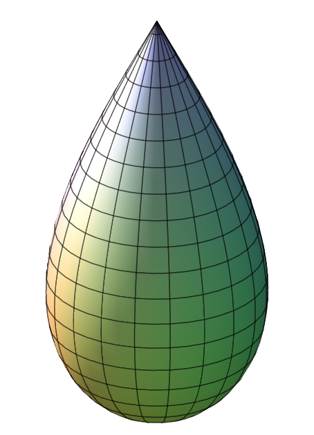
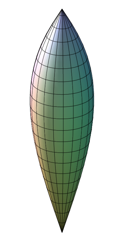
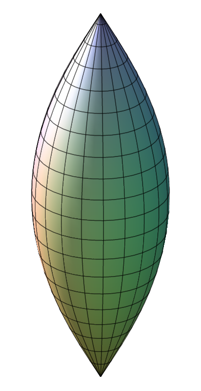
Figure 5: The teardrop and football (with different angles) solitons with non-constant curvature, and a constant curvature football with equal angles (courtesy of D. Ramos [208]).

Fix a smooth compact surface $M$, along with a conformal, or equivalently, complex structure $J$. A divisor $D$ is now a collection of distinct points $\{p_{1},\ldots,p_{N}\}\subset M$ and the associated class $c_{1}(M,J)-\sum(1-\beta_{j})p_{j}$, that can be thought of as a modified Euler characteristic, is

$$2-2g(M)-\sum_{j=1}^{N}(1-\beta_{j}).$$ (4.7)

In particular, this is now a number, and so the cohomological condition (3.12) is always satisfied. In a local conformal coordinate chart near each $p_{j}$, $g=\sqrt{-1}\gamma_{j}dz\otimes\overline{dz}=\sqrt{-1}\gamma_{j}|dz|^{2}$, with $\gamma=|z|^{2\beta_{j}-2}F_{j}$ and $F_{j}$ bounded. Suppose that $g$ has constant curvature away from the cone points. The Poincaré–Lelong formula asserts that $-\Delta_{g}\log|z|$ is a multiple of the delta function at $\{z=0\}$ (this can be seen by excising a small neighborhood near the cone point and using Stokes’ formula). Together with the standard formula for the scalar curvature, $K_{g}=-\Delta_{g}\log\gamma$ (up to a constant factor), it follows that

$$K_{g}-2\pi\sum(1-\beta_{i})\delta_{p_{i}}=\hbox{const},$$ (4.8)

with the constant given by (4.7). The existence in the nonpositive regime uses standard methods as in the smooth setting, e.g., the variational method of Berger [17], or the method of sub- and super-solutions used by Kazdan–Warner [145]. A somewhat surprising discovery of Troyanov was the sufficient condition

$$\beta_{j}-1>\sum_{i\neq j}\beta_{i}-1,\quad\hbox{for each $j=1,\ldots,N$,}$$ (4.9)

for existence in the positive case, that followed by generalizing Moser’s inequality [185, 186] to the singular setting. For instance, if $N=2$, this is violated when $\beta_{1}\not=\beta_{2}$. As observed by Ross–Thomas, this condition can be rephrased by saying that the Futaki invariant of the pair $(M,\sum(1-\beta_{i})p_{i})$ has the right sign, or that the pair is slope (poly)stable [211, Theorem 8.1] (see [211, Remark 8.4] for a careful treatment of the equality case in (4.9)). The only additional unobstructed pair is $N=2$ with $\beta_{1}=\beta_{2}$, and such a csc metric can be constructed explicitly using ODE methods; when $\beta_{1}\not=\beta_{2}$ or $N=1$ one can still construct a shrinking Ricci soliton [130] (see also [26, 208]). These are depicted in Figure 5. We also remark that [141] and Berman’s work gave a new proof of Troyanov’s original results [18], and Berndtsson’s work gave a new approach to uniqueness [25]. Finally, the higher regularity of such a metric was only obtained much later [141], as a corollary of Theorem 3.16.

The variational approach has recently been extended considerably through the work of Malchiodi et al. to allow angles $\beta>1$, even when coercivity fails, see, e.g., [15, 56]. For some higher regularity results also in this regime we refer to [177].

4.5 Existence theorem for positive curvature

The following essentially optimal existence result in the positive case is due to [141]. It parallels and generalizes Tian’s theorem from the smooth setting [245, §6]. We postpone the definition of properness to §5.2.

Theorem 4.13.

(Kähler–Einstein edge metrics with positive Ricci curvature) Let $(M,\omega_{0})$ be a compact Kähler manifold, $D\subset M$ a smooth divisor, and suppose that $\beta\in(0,1]$ and $\mu>0$ are such that

$$c_{1}(M)-(1-\beta)[D]=\mu[\omega_{0}],$$

and that the twisted K-energy $E_{0}^{\beta}$ is proper. Then, there exists a Kähler–Einstein edge metric $\omega_{\varphi_{\hbox{\sml KE}}}$ with Ricci curvature $\mu$ and with angle $2\pi\beta$ along $D$, that is unique up to automorphisms that preserve $D$. This metric is polyhomogeneous, namely, $\varphi_{\hbox{\sml KE}}$ admits a complete asymptotic expansion with smooth coefficients as $r\to 0$ of the form

$$\varphi_{\hbox{\sml KE}}(r,\theta,z_{2},\ldots,z_{n})\sim\sum_{j,k\geq 0}\sum_{\ell=0}^{N_{j,k}}a_{jk\ell}(\theta,z_{2},\ldots,z_{n})r^{j+k/\beta}(\log r)^{\ell},$$ (4.10)

where locally $D$ is cut-out by $z_{1}$, $r=|z_{1}|^{\beta}/\beta$ and $\theta=\arg z_{1}$, and with each $a_{jk\ell}\in C^{\infty}$. There are no terms of the form $r^{\zeta}(\log r)^{\ell}$ with $\ell>0$ if $\zeta\leq 2$. In particular, $\varphi_{\hbox{\sml KE}}\in\mathcal{A}^{0}\cap\mathcal{D}^{0,\frac{1}{\beta}-1}_{w}$, i.e., $\omega_{\varphi_{\hbox{\sml KE}}}$ has infinite conormal regularity, and is $(\frac{1}{\beta}-1)$-Hölder continuous with respect to the reference edge metric $\omega$.

A parallel result in the snc case can be stated [175, 176]. In fact, the a priori estimates of [141] apply to the snc case without any change. The essential new difficulty, however, as compared to the smooth divisor case, is to extend the linear theory to one with crossing edges. This is new even in the real setting, and goes beyond the original methods of Mazzeo [172]. A different approach to the existence, avoiding such linear theory, but producing only $\mathcal{D}^{0,0}_{w}$ solutions without Hölder estimates on the metric (or even continuity of the metric up to $D$) nor higher regularity, and under the assumption that a $C^{0}$ (or even a weaker) solution exists, has been developed by Guenancia–Pǎun [127] (a similar result is obtained by Yao [265] who derives the $C^{0}$ estimate based on the approximation scheme of [63, 248]), as described in §4.1. Their approach starts from the $C^{0}$ solution constructed by Berman [18] and [141], and produces a $\mathcal{D}^{0,0}_{w}$ estimate by a careful approximation by smooth metrics. Finally, the uniqueness is due to Berndtsson [25].

Strategy of proof of Conjecture 4.2 and Theorem 4.13.

The proof uses results from Sections 3, 6, and 7. We now describe how these results piece together.

Solving the KE equation is equivalent to solving the Monge–Ampère equation (3.7). We embed this equation in a one-parameter family of equations (6.3), called the Ricci continuity path (Ricci CP), and define as usual the set

$$I:=\{s\in(-\infty,\mu]\,:\,\hbox{\eqref{RCMEq} with parameter value $s$ admits a solution in $\mathcal{D}_{w}^{0,\gamma}\cap C^{4}(M\setminus D)$}\}.$$

Equation (6.3) with parameter value $\mu$ is precisely (3.7). By Proposition 6.1, there exists some $S>-\infty$ such that $(-\infty,S)\subset I$, so that $I$ is not empty. Furthermore, $I$ is open. As a matter of fact, the linearization of (6.3) at the parameter value $s$ is given by $\Delta_{\omega_{\varphi(s)}}+s$. This is clearly invertible when $s<0$, and is also invertible when $s>0$ since, as shown in §7.1, the first eigenvalue of $\Delta_{\omega_{\varphi(s)}}+s$ is positive whenever $s\in(0,\mu)$. Invertibility at $s=0$ follows by working on the orthogonal complement of the constants [9]. Thus, Theorem 3.7 (i) yields the openness. The fact that $I$ is closed (and hence equal to $(-\infty,\mu]$) follows from Theorem 6.3. Thus, (3.7) admits a solution in $\mathcal{D}_{w}^{0,\gamma}\cap C^{4}(M\setminus D)$. Theorem 3.16 implies that the solution is polyhomogeneous and belongs to $\mathcal{A}^{0}_{\operatorname{phg}}$; Equation (3.24) further implies the precise regularity statements about the solution. ∎

Note that the proof gives a new and unified proof for the classical results of Aubin, Tian and Yau, on the existence of smooth KE metrics, in that it uses a single continuity method for all signs of $\mu$. This point is discussed in detail in §6.2.

Finally, consider the special case that $M$ is Fano and $D$ is a smooth anticanonical divisor (the existence of such a divisor is highly nontrivial, we refer to Problem 8.9 and the discussion there). Then, as noted by Berman [18], the twisted K-energy is proper for small $\mu=\beta>0$. Theorem 4.13 thus gives the following corollary conjectured by Donaldson [101].

Corollary 4.14.

Let $M$ be a Fano manifold, and suppose that there exists a smooth anticanonical divisor $D\subset M$. Then there exists some $\beta_{0}\in(0,1]$ such that for all $\beta\in(0,\beta_{0})$ there exists a KEE metric with angle $2\pi\beta$ along $D$ and with positive Ricci curvature equal to $\beta$.

Li–Sun [157] observed that the exact same arguments actually prove existence also in the plurianticanonical setting: supposing there exists a smooth divisor $D$ in $|-mK_{M}|$ (this always holds if $M$ is Fano and $m\in{\mathbb{N}}$ is sufficiently large by Kodaira’s theorem), there exists a small $\beta_{0}>0$ such that there exists a KEE metric with $\beta\in(1-\frac{1}{m},1-\frac{1}{m}+\beta_{0})$ along $D$ and with $\mu=1-(1-\beta)m$.

5 Energy functionals

The Mabuchi energy was crucial in stating the main existence theorem (Theorem 4.13). The purpose of this section is to describe several energy functionals, including the Mabuchi energy, that cast the Kähler–Einstein (edge) problem as a variational one. (The variational approach can be applied to much more general settings, and we do not seek full generality, for which we refer to Berman et al. [18, 22, 23].) First, in §5.1, we describe the Aubin energy functionals, that are nonlinear generalizations of the $W^{1,2}$-seminorm. Using these functionals it is easy to construct the Ding functional whose Euler–Lagrange equation is the inhomogeneous Monge–Ampère equation. Using the Aubin energies, one can then define a notion of relative compactness of level sets of an energy functional, and this leads to a calculus of variations formulation of the Kähler–Einstein problem in §5.2. Both the Mabuchi and Ding energies can be defined in a more conceptual way, using Bott–Chern forms. We describe this in detail in §5.4 since we are not aware of a single easy-to-read reference for this (we refer to [198, 227] for the related Deligne pairing formalism). In §5.3 we also describe other natural functionals, the Kähler–Ricci energies, that lend themselves to a similar description, mainly to illustrate the richness of the theory, but also to show that there are many more-or-less equivalent functionals whose variational theory underlies the KE problem. Subsection 5.5 describes a relation between the Ding energy and the Mabuchi energy, involving the Legendre transform. Building on the preceeding subsections, in §5.6 we prove the equivalence, in suitable senses, of the Ding, Mabuchi, and Kähler–Ricci energies.

5.1 Nonlinear Dirichlet energies and the Berger–Moser–Ding functional

The most basic functionals, going back to the work of Aubin [9], are defined by

$$I(\eta,\eta_{\varphi}) =\frac{1}{V}\int_{M}\sqrt{-1}\partial\varphi\wedge\bar{\partial}\varphi\wedge\sum_{l=0}^{n-1}\eta^{n-1-l}\wedge\eta_{\varphi}^{l}=\frac{1}{V}\int_{M}\varphi(\eta^{n}-\eta^{n}_{\varphi}),$$ (5.1)

$$J(\eta,\eta_{\varphi}) =\frac{V^{-1}}{n+1}\int_{M}\sqrt{-1}\partial\varphi\wedge\bar{\partial}\varphi\wedge\sum_{l=0}^{n-1}(n-l)\eta^{n-l-1}\wedge\eta_{\varphi}^{l}.$$

The functionals $I,J$, and $I-J$ are all equivalent (and hence the latter is nonnegative), in the sense that $\frac{1}{n}J\leq I-J\leq\frac{n}{n+1}I\leq nJ.$ Granted, these might not look so ‘basic’ at a first glance. Let us give some motivation to these definitions.

The first motivation comes from the calculus of variations: is there a sort of nonlinear Dirichlet energy whose Euler–Lagrange equation is (2.3)? In the case $n=1$ such an energy was studied by Berger and Moser [17, 186]

$$F(\eta,\eta_{\varphi})=\begin{cases}\displaystyle\frac{1}{V}\int\frac{1}{2}\sqrt{-1}\partial\varphi\wedge\bar{\partial}\varphi-\frac{1}{V}\int\varphi\eta-\frac{1}{\mu}\log\frac{1}{V}\int e^{f_{\eta}-\mu\varphi}\eta,&\hbox{for $\mu\neq 0$,}\cr\displaystyle\frac{1}{V}\int\frac{1}{2}\sqrt{-1}\partial\varphi\wedge\bar{\partial}\varphi-\frac{1}{V}\int\varphi\eta+\frac{1}{V}\int\varphi e^{f_{\eta}}\eta,&\hbox{for $\mu=0$.}\cr\end{cases}$$ (5.2)

(Recall the definition of $f_{\eta}$ (3.9).) Its critical points are precisely constant scalar curvature metrics in the conformal class. It is straightforward to generalize in higher dimensions the last term to $\frac{1}{\mu}\log\frac{1}{V}\int e^{f_{\eta}-\mu\varphi}\eta^{n}$ (respectively, $\frac{1}{V}\int\varphi e^{f_{\eta}}\eta^{n}$) so that its variational derivative comes out to be the right hand side of (2.3) (up to the implicit normalization that the integral of the right hand side is 1). How to replace the first two terms so that the resulting Euler–Lagrange equation comes out right? This amounts to finding a functional whose differential is exactly minus the Monge–Ampère operator, i.e., the left hand side of (2.3). This is precisely the functional $-L$ (recall (4.2) and the line following it). Decomposing $-L$ into two terms, one of which is $-\frac{1}{V}\int\varphi\eta^{n}$, yields precisely $J$ as the second term! (Incidentally, this also explains why $L$, defined in (4.2), is called the Aubin–Mabuchi functional.)

Thus, the Euler–Lagrange equation for the Berger–Moser–Ding energy (or Ding energy for short) [88]

$$F^{\beta}(\eta,\eta_{\varphi})=\begin{cases}\displaystyle J(\eta,\eta_{\varphi})-\frac{1}{V}\int\varphi\eta^{n}-\frac{1}{\mu}\log\frac{1}{V}\int e^{f_{\eta}-\mu\varphi}\eta^{n},&\hbox{for $\mu\neq 0$,}\cr\displaystyle J(\eta,\eta_{\varphi})-\frac{1}{V}\int\varphi\eta^{n}+\frac{1}{V}\int e^{f_{\eta}}\eta^{n},&\hbox{for $\mu=0$,}\cr\end{cases}$$ (5.3)

is precisely (3.7).

5.2 A nonlinear variational problem

This brings us to a second motivation for $J$. As we just noticed, $-L(\varphi)=J(\eta,\eta_{\varphi})-\int\varphi\eta^{n}$. Recall that $\pm L$ (4.2) is a distance function for the Mabuchi metric. Thus, it is tempting to think of $J$ as a sort of approximate distance function. This is of course not quite true, since the submanifold $\{\varphi\in\mathcal{H}^{e}_{\omega}\,:\,\int\varphi\eta^{n}=0\}$ of $\mathcal{H}^{e}_{\omega}$ is not totally geodesic. But ignoring this subtlety, one is then tempted to think of $J$ as a good way to define coercivity for our nonlinear problem on $\mathcal{H}_{\omega}^{e}$; of course this temptation also arises from the first motivation discussed earlier. Following Tian [243], one says a functional $E$ on $\mathcal{H}_{\omega}\times\mathcal{H}_{\omega}$ is proper provided that it dominates $J$ (or, by their equivalence, $I$ or $I-J$) on each $\mathcal{H}_{\omega}$ slice. This is an analogue of the standard assumption in the direct method in the calculus of variations, namely that sublevel sets (of $E$) are compact. In particular, if $E$ is proper, a sublevel set of $E$ is contained in some sublevel set of $J$. Theorem 4.13 can be recast as a nonlinear analogue of the fundamental theorem of the direct method (cf. [231, Theorem 1.1]) in this setting, justifying the definition of properness.

Theorem 5.1.

Suppose that $F^{\beta}(\omega,\,\cdot\,)$ is proper on $\mathcal{H}^{e}_{\omega}$. Then it is bounded from below, and its infimum is attained at a solution of (2.3).

For the proof we refer to [141, Theorem 2] (that proof assumes that the Mabuchi functional $E^{\beta}_{0}$ is proper, however the arguments are identical; a conceptual proof of the equivalence coercivity of $F^{\beta}$ and that of $E_{0}^{\beta}$ is given in Theorem 5.11 (ii), although a direct proof (i.e., one that does not use the existence of a minimizer) of equivalence of the properness of these functionals seems to be unknown). The special case when $\beta=1$ goes back to Ding–Tian [90] and Tian [243] (see also [247, §2.2] for a generalization that allows for automorphisms). On the other hand, Berman showed that under the assumption in the theorem the infimum is attained within the larger set $\mathrm{PSH}(M,\omega)\cap C^{0}(M)$, and while it is easy to see that the minimizer is contained in $C^{\infty}(M\setminus D)$ by local ellipticity and the usual arguments as in the smooth case, the proof that the minimizer lies in $\mathcal{H}^{\epsilon}_{\omega}$ [141] relies on the Ricci continuity method, as described in §6–7.

5.3 The staircase energies and Kähler–Ricci energies

A generalization of the Aubin energy $J$ (5.1) was introduced in [213, (6)],

$$I_{k}(\omega,{\omega_{\varphi}})=\frac{V^{-1}}{k+1}\int_{M}\varphi(k\omega^{n}-\sum_{l=1}^{k}\omega^{n-l}\wedge{\omega_{\varphi}}^{l}).$$ (5.4)

Note that $I_{n}=J,\;I_{n-1}=({(n+1)J-I})/n$. These functionals are nonnegative (see (5.5) below) and are related to, but different from, functionals defined by Chen–Tian [67]—see [216, p. 133]. The functionals $I_{k}$ can be thought of as gradual nonlinear generalizations of the Dirichlet energy that interpolate between the latter and $J$. In fact, $I_{1}$ is simply a multiple of the Dirichlet energy $\int\sqrt{-1}\partial\varphi\wedge\bar{\partial}\varphi\wedge\omega^{n-1}$, and increasing $k$ is analogous to climbing a staircase (see [216, p. 132] for a pictorial description) where $I_{k}$ incorporates one additional ‘mixed’ term proportional to $\int\sqrt{-1}\partial\varphi\wedge\bar{\partial}\varphi\wedge\omega^{n-k}\wedge{\omega_{\varphi}}^{k-1}$; indeed, by integrating by parts,

$$I_{k}(\omega,{\omega_{\varphi}})=\frac{1}{V}\int_{M}\sqrt{-1}\partial\varphi\wedge\bar{\partial}\varphi\wedge\sum_{l=0}^{k-1}\frac{k-l}{k+1}\omega^{n-1-l}\wedge{\omega_{\varphi}}^{l}.$$ (5.5)

The definition (5.4) certainly makes sense for pairs of smooth Kähler forms, and by Theorem 3.10 (i) and the continuity of the mixed Monge–Ampère operators on $\mathrm{PSH}(M,\omega_{0})\cap C^{0}(M)$ [16, Proposition 2.3], these functionals can be uniquely extended to pairs $(\omega_{\varphi_{1}},\omega_{\varphi_{2}})$, with $\varphi_{1},\varphi_{2}\in\mathcal{H}^{e}_{\omega}$ with $\omega$ the reference edge metric as in (3.5). Thus, these functionals are well-defined on $\mathcal{H}^{e}_{\omega}\times\mathcal{H}^{e}_{\omega}$. Moreover, (5.5) is still justified for edge metrics: working on a tubular neighborhood of $D$ the boundary term one obtains from integrating by part in (5.4) tends to zero with the radius of the neighborhood about $D$.

As we just saw, the functionals $I_{k}$ are a natural generalization of the Dirichlet energy on the one hand, and Aubin’s $J$ functional on the other. It turns out that $I_{k}$ play a role in describing a scale of energy functionals $E_{k}$ that similarly depend gradually on additional ‘mixed terms’ as $k$ increases, loosely speaking. This can be made precise using the language of Bott–Chern forms that we review in §5.4. Another, more down to earth way, of defining this functional is as follows.

Denote the normalized elementary symmetric polynomials of the eigenvalues of the twisted Ricci form $\hbox{\rm Ric}\,\,\eta-(1-\beta)[D]$ (with respect to $\eta$) by

$$\sigma^{\beta}_{k}(\eta)=\frac{(\hbox{\rm Ric}\,\,\eta-(1-\beta)[D])^{k}\wedge\eta^{n-k}}{\eta^{n}},\quad k=1,\ldots,n,$$

and their average (which is independent of the representative of $[\eta]$) over $(M,\omega^{n})$ by

$$\mu^{\beta}_{k}:=\frac{(c_{1}-(1-\beta)c_{1}(L_{D}))^{k}\cup[\eta]^{n-k}([M])}{[\eta]^{n}([M])}.$$ (5.6)

When $k=1$, $\sigma_{1}^{\beta}(\eta)=s_{\eta}/n=\hbox{\rm tr}_{\eta}(\hbox{\rm Ric}\,\,\eta-(1-\beta)[D])/n$, where $s_{\beta}(\eta)$ denotes the twisted scalar curvature of $\eta$. When $k=n$ this is $\det_{\eta}(\hbox{\rm Ric}\,\,\eta-(1-\beta)[D])$, the determinant of the twisted Ricci curvature with respect to the metric.

A straightforward generalization of a theorem of the author from the case $\beta=1$ [213, Proposition 2.6] yields the following.

Proposition 5.2.

Let $k\in\{0,\ldots,n\}$. Suppose $\mu[\eta]=c_{1}-(1-\beta)c_{1}(L_{D})$. The 1-form

$$\eta\mapsto\Big{[}\Delta_{\eta}\sigma^{\beta}_{k}(\eta)-\frac{n-k}{k+1}\Big{(}\sigma^{\beta}_{k+1}(\eta)-\mu^{\beta}_{k+1}\Big{)}\Big{]}\eta^{n}$$

is exact. Its potential, considered as a function on $\mathcal{H}_{\eta}^{e}\times\mathcal{H}_{\eta}^{e}$, is given by

$$\mu^{-k}E^{\beta}_{k}(\eta,\eta_{\varphi})=E^{\beta}_{0}(\eta,\eta_{\varphi})+\mu I_{k}(\eta_{\varphi},\mu^{-1}\hbox{\rm Ric}\,\,\!\eta_{\varphi}-\mu^{-1}(1-\beta)[D])-\mu I_{k}(\eta,\mu^{-1}\hbox{\rm Ric}\,\,\!\eta-\mu^{-1}(1-\beta)[D]),$$ (5.7)

uniquely determined by the normalization $E_{k}^{\beta}(\eta,\eta)=0$.

Proof.

As remarked earlier, $I_{k}$ is continuous in the topology of uniform convergence (on the level of Kähler potentials) by a result of Bedford–Taylor. By definition (see the second part of Definition 3.2, (3.20), and (3.17)), $\hbox{\rm Ric}\,{\omega_{\varphi}}-(1-\beta)[D]$ admits a continuous Kähler potential with respect to $\omega$, and moreover this potential can be suitably uniformly approximated. Smoothly approximate $(\omega,{\omega_{\varphi}})$ uniformly while approximating $\hbox{\rm Ric}\,{\omega_{\varphi}}-(1-\beta)[D]$ uniformly on the level of potentials. Thus, it suffices to verify the proposition when the Kähler forms are smooth, when integration by parts, precisely those in the proof in the smooth case [213], are justified. But then the proof in the smooth case can be applied verbatim, with the definition of the twisted Ricci potential as in (3.9) (recall $f_{\omega}$ is continuous for all $\beta$) making the proof consistent with the introduction of the terms $(1-\beta)[D]$ in the right hand side of (5.7). ∎

Similar arguments allow to generalize the following formula of Tian [241] from the smooth case.

Lemma 5.3.

Let $\eta,\eta_{\varphi}\in\mathcal{H}^{e}_{\omega}$. One has,

$$E^{\beta}_{0}(\eta,\eta_{\varphi})=\frac{1}{V}\int_{M}\log\frac{\eta_{\varphi}^{n}}{\eta^{n}}\eta_{\varphi}^{n}-\mu(I-J)(\eta,\eta_{\varphi})+\frac{1}{V}\int_{M}f_{\eta}(\eta^{n}-\eta_{\varphi}^{n}).$$ (5.8)

The functionals $E_{0}$ and $E_{n}$ were introduced by Mabuchi [167] and Bando–Mabuchi [14], while the remaining ones by Chen–Tian [67]. Formula (5.7) shows that the $E_{k}$ interpolate between $E_{0}$ and $E_{n}$, to wit [213, (17)]

$$E^{\beta}_{0}(\eta,\eta_{\varphi}) =((1-\hbox{$\frac{l}{k+1}$})E_{0}+\hbox{$\frac{l}{k+1}$}E_{n})(\eta,\eta_{\varphi})+(I_{k}-\hbox{$\frac{l}{k+1}$}J)(\eta_{\varphi},\mu^{-1}\hbox{\rm Ric}\,\,\!\eta_{\varphi}-(1-\beta)[D]/\mu)\qquad$$

$$\qquad-(I_{k}-\hbox{$\frac{l}{k+1}$}J)(\eta,\hbox{\rm Ric}\,\,\eta),\quad\forall\,l\in\{0,\ldots,k+1\}.$$

Since $E_{0}$ is known as the K-energy or Kähler energy, and $E_{n}$ as the Ricci energy, it is natural, following [213], to refer to $E_{k}$ as the Kähler–Ricci energies.

The Ricci energy is special. It lends a geometric interpretation to the Ding functional, via the inverse Ricci operator, in the sense of [214, §9]. That is, suppose that (3.12) holds with $\mu=1$. Define by $\hbox{\rm Ric}\,^{-1}_{\beta}:\mathcal{H}_{\omega}^{\epsilon}\rightarrow\mathcal{H}_{\omega}^{\epsilon}$ the twisted inverse Ricci operator, by letting $\hbox{\rm Ric}\,^{-1}_{\beta}\eta:=\chi$ be the unique Kähler form cohomologous to $\eta$ satisfying $\hbox{\rm Ric}\,\chi-(1-\beta)[D]=\eta$. Such a unique form exists by Conjecture 4.2, since this equation can be written as a Monge–Ampère equation of identical form to that of the equation for a Ricci flat Kähler edge metric.

Proposition 5.4.

One has $(\hbox{\rm Ric}\,_{\beta}^{-1})^{\star}E^{\beta}_{n}=F^{\beta}.$

Again, the proof is a simple adaptation of the proof in the smooth case [214, Proposition 10.4], following the arguments in the proof of Proposition 5.2 above.

5.4 Bott–Chern forms

In this subsection we will describe the theory of Bott–Chern forms and energy functionals, inspired by work of Bott and Chern [37] and developed by Donaldson and Bismut–Gillet–Soulé [92, 29]. This will be applied to showing that the functionals $E_{k}^{\beta}$ have an expression in terms of Bott–Chern forms, slightly generalizing but very closely following the discussion in [216, §4.4.5].

The main idea of Bott–Chern forms is that given a moduli space of Hermitian metrics on a bundle one may construct canonically defined “universal” functions on it associated to curvature. These functions arise via a “potential” for the curvature form of a “universal” bundle over the whole moduli space.

Let $E\rightarrow M$ be a holomorphic vector bundle of rank $r$. A vector bundle represents a $\check{\hbox{C}}$ech cohomology class in $H^{1}(M,\mathcal{O}_{M}(GL(r,{\mathbb{C}})))$. Here by $\mathcal{O}_{M}(GL(r,{\mathbb{C}}))$ we mean the sheaf of germs of holomorphic functions to $GL(r,{\mathbb{C}})$. When $r=1$ it is denoted by $\mathcal{O}_{M}^{\star}$. Let us identify $E$ with its $\check{\hbox{C}}$ech class representative, i.e., by a collection of transition functions $g=\{g_{\alpha\beta}\}$ that are holomorphic maps from the intersection of any two coordinate neighborhoods $U_{\alpha},U_{\beta}\subset M$ to $GL(r,{\mathbb{C}})$, $g_{\alpha\beta}:U_{\alpha}\cap U_{\beta}\rightarrow GL(r,{\mathbb{C}})$, satisfying the $\check{\hbox{C}}$ech cocycle conditions [124, p. 66]

$$(\delta g)_{\alpha\beta\gamma}:=g_{\alpha\beta}\cdot g_{\beta\gamma}\cdot g_{\gamma\alpha}=\hbox{\rm I}.$$

Note that here the groups comprising the sheaf have a multiplicative structure (and not an additive one) and hence $\delta g=\hbox{\rm I}$ expresses closedness, i.e., $[g]$ represents a $\check{\hbox{C}}$ech cohomology class.

Denote by $\mathcal{H}_{E}$ the space of all Hermitian metrics on $E$. Let ${\operatorname{Herm}}(r)$ denote the space of positive Hermitian $r\times r$ matrices. Any Hermitian metric $H\in\mathcal{H}_{E}$ can be represented by smooth maps $H_{\alpha}:U_{\alpha}\rightarrow$ Herm$(r)$ such that with respect to local bases of sections one has $(H_{\alpha})_{i\bar{j}}=(g_{\alpha\beta})_{ik}(H_{\beta})_{k\bar{l}}\overline{(g_{\alpha\beta})_{jl}}$, or simply $H_{\alpha}=g_{\alpha\beta}^{\star}H_{\beta}g_{\alpha\beta}$. This is summarized in the notation $H=\{H_{\alpha}\}$.

To every $H\in\mathcal{H}_{E}$ there is associated a unique complex connection $D_{H}$. For a general holomorphic vector bundle the connection $D_{H}$ is a 1-form on $M$ with values in the bundle $\hbox{\rm End}(E)$ of endomorphisms of $E$. One may write globally

$$D_{H}=H^{-1}\circ\partial\circ H.$$

The derivation of this formula follows the same argument as in the line bundle case. The exact meaning of how to understand this and other similar expressions involving compositions of endomorphisms and differential operators will be explained in detail below in several computations. With respect to a local holomorphic frame $e_{1},\ldots,e_{r}$ over $U_{\alpha}\subset M$ the endomorphism $H$ may be represented by a matrix and one has the special expression $(D_{H}|_{U_{\alpha}})_{j}^{i}=\partial h_{j\bar{l}}\cdot h^{\bar{l}i}$. This expression is not valid with respect to an arbitrary frame.

The global expression for the curvature is then

$$F_{H}:=D_{H}\circ D_{H}=\bar{\partial}\circ H^{-1}\circ\partial\circ H.$$ (5.9)

Implicit in this notation as well as in the sequel is the convention of working with endomorphisms with values in the exterior algebra of differential forms on $M$. Locally with respect to a holomorphic frame one has the special expression $F_{H}|_{U_{\alpha}}=\bar{\partial}(\partial h_{j\bar{l}}\cdot h^{\bar{l}i})$. This expression is not valid with respect to an arbitrary frame. However it demonstrates that $F_{H}$ is $(1,1)$-form on $M$ (with values in $\hbox{\rm End}(E)$), since the type is independent of the choice of frame.

Let $\phi$ denote an elementary symmetric polynomial on $gl(r,{\mathbb{C}})\times\cdots\times gl(r,{\mathbb{C}})$ ($p$ times) that is invariant under the adjoint action of $GL(r,{\mathbb{C}})$ (conjugation). The idea behind Chern classes is that one may plug into such polynomials matrices that have differential forms as their entries, for example $F_{H}$. Since the polynomials are $GL(r,{\mathbb{C}})$-invariant one obtains a differential form that is invariant under a change of local trivializations for the bundle, hence is intrinsically defined. Moreover it turns out that such forms are closed, hence define intrinsic cohomology classes that depend only on the complex structure of $E\rightarrow M$.

Now we come back to our original task of constructing functions on $\mathcal{H}_{E}$. One may show that $\phi(F_{H}):=\phi(F_{H},\ldots,F_{H})$ is a closed $2p$-form. It certainly depends on the metric $H$, however its cohomology class in $H^{2p}(M,{\mathbb{Z}})$ does not. This means that the difference

$$\phi(F_{H_{0}})-\phi(F_{H_{1}})$$

is exact. Moreover, and here we arrive at the main point of Bott–Chern theory, one may find a $(p-1,p-1)$-form $\hbox{\bf BC}(\phi;H_{0},H_{1})$, well-defined up to $\partial$- and $\bar{\partial}$-exact forms, such that

$$\bar{\partial}\partial\hbox{\bf BC}(\phi;H_{0},H_{1})=\phi(F_{H_{1}})-\phi(F_{H_{0}}).$$

The form $\hbox{\bf BC}(\phi;H_{0},H_{1})$ may then be integrated against a $(n-p+1,n-p+1)$-form on $M$ to give a number. Fixing $H_{0}$ and letting $H_{1}$ vary we therefore obtain a function on $\mathcal{H}_{E}$ as desired. And, if $p-1=n$, we even do not need to make a choice of such a form in order to integrate (this will be the case in our applications). We now show how to construct the Bott–Chern form $\hbox{\bf BC}(\phi;H_{0},H_{1})$. The proof below is a slow pitch version of the orignal one.

Proposition 5.5.

(See [92, Proposition 6].) Let $\phi$ be a $GL(r,{\mathbb{C}})$-invariant elementary symmetric polynomial. Given $H_{0},H_{1}\in\mathcal{H}_{E}$ and any path $\{H_{t}\}_{t\in[0,1]}$ in $\mathcal{H}_{E}$ connecting them, the $(p-1,p-1)$-form

$$\hbox{\bf BC}(\phi;H_{0},H_{1}):=p(\sqrt{-1})^{p-1}\int_{[0,1]}\phi(H_{t}^{-1}\dot{H}_{t},F_{H_{t}},\ldots,F_{H_{t}})dt\quad\hbox{\rm mod}\quad{\operatorname{Im}}\partial+{\operatorname{Im}}\bar{\partial},$$ (5.10)

is well-defined, namely does not depend on the choice of path. In addition,

$$\hbox{\bf BC}(\phi;H_{0},H_{1})+\hbox{\bf BC}(\phi;H_{1},H_{2})+\hbox{\bf BC}(\phi;H_{2},H_{0})=0,$$ (5.11)

and

$$\bar{\partial}\partial\hbox{\bf BC}(\phi;H_{0},H_{1})=\phi(F_{H_{1}})-\phi(F_{H_{0}}).$$ (5.12)

Notice that the first argument of $\phi$ is an endomorphism while the rest of its arguments are endomorphism-valued $2$-forms.

Proof.

Note that $\hbox{\bf BC}(\phi;H_{0},H_{1})$ is given by integration over a path connecting $H_{0}$ and $H_{1}$ of a globally defined 1-form on $\mathcal{H}_{E}$ with values in $(p-1,p-1)$-forms on $M$. We call this form $\theta$. To show independence of path we show that this form is closed modulo $\partial$- and $\bar{\partial}$-exact terms. Let $H\in\mathcal{H}_{E}$. Let $h,k\in T_{H}\mathcal{H}_{E}$ and extend them to constant vector fields near $H$. Then,

$$d\theta(h,k)=k\,\theta|_{H}(h)-h\,\theta|_{H}(k).$$ (5.13)

First we obtain an expression for the infinitesimal change of the curvature under a variation of a Hermitian metric. Write $H+tk=H\circ(\hbox{\rm I}+tH^{-1}k)=:H\circ f$. We write $\circ$ to emphasize that composition of endomorphisms is taking place (in coordinates multiplication of matrices). According to (5.9) we have

$$F_{H\circ f} =\bar{\partial}\big{(}(H\circ f)^{-1}\circ\partial(H\circ f)\big{)}$$ (5.14)

$$=\bar{\partial}\big{(}f^{-1}\circ(H^{-1}\circ\partial H)\circ f+f^{-1}\circ\partial f\big{)}$$

$$=\bar{\partial}\circ f^{-1}\circ D_{H}^{1,0}\circ f.$$

Here it should be emphasized that $D_{H}$ decomposes according to type (of its 1-form part) into $D_{H}^{1,0}$ and $D_{H}^{0,1}$ and that while originally the connection $D_{H}$ was defined on $E$ it may be extended naturally to $\hbox{\rm End}(E)$ and it is this extension that we use in the equation above ($f$ is a section of $\hbox{\rm End}(E)$ and not of $E$). The same applies to the operator $\bar{\partial}$ that we also extend to act on $\hbox{\rm End}(E)$. To understand the last equation better we let the endomorphism it defines act on a holomorphic section $s$ of $E$, and compute:

$$F_{H\circ f}s =\bar{\partial}\circ f^{-1}\circ D_{H}^{1,0}(fs)$$

$$=\bar{\partial}\circ f^{-1}\circ\big{(}(D_{H}^{1,0}f)s+fD_{H}^{1,0}s\big{)}$$

$$=\Big{(}\bar{\partial}\big{(}f^{-1}(D_{H}^{1,0}f)\big{)}+\bar{\partial}\circ D_{H}^{1,0}\Big{)}s.$$

Therefore we write

$$F_{H\circ f}=F_{H}+\bar{\partial}\big{(}f^{-1}(D_{H}^{1,0}f)\big{)},$$

and the second term should be understood to be distinct from (LABEL:CircCurvatureEq). This subtle notational issue can be a cause for great confusion when consulting the literature on vector bundles and Yang-Mills theory. Putting now $f=\hbox{\rm I}+tH^{-1}k$ we obtain

$$F_{H+tk}=F_{H}+t\bar{\partial}\big{(}D_{H}^{1,0}(H^{-1}k)\big{)}+O(t^{2}).$$

Hence the first term in (5.13) is given by

$$\frac{1}{p(\sqrt{-1})^{p-1}}k\theta|_{H}(h) =\frac{d}{dt}\Big{|}_{0}\phi((H+tk)^{-1}h,F_{H+tk},\ldots,F_{H+tk})$$ (5.15)

$$=\phi(-\sqrt{-1}Hk\sqrt{-1}Hh,F_{H},\ldots,F_{H})$$

$$\quad+{\text{\sum}}\phi(\sqrt{-1}Hh,F_{H},\ldots,\bar{\partial}D_{H}^{1,0}(\sqrt{-1}Hk),\ldots,F_{H}).$$

Therefore one has, putting $\sigma=\sqrt{-1}Hh,\;\tau=\sqrt{-1}Hk$,

$$\frac{1}{p(\sqrt{-1})^{p-1}}d\theta(h,k) =\phi([\sigma,\tau],F_{H},\ldots,F_{H})+{\text{\sum}}\phi(\sigma,F_{H},\ldots,\bar{\partial}D_{H}^{1,0}\tau,\ldots,F_{H})$$ (5.16)

$$\quad-{\text{\sum}}\phi(\tau,F_{H},\ldots,\bar{\partial}D_{H}^{1,0}\sigma,\ldots,F_{H}).$$

$\sigma$ and $\tau$ are sections of the endomorphism bundle of $E$. Note that as operators on this bundle one has

$$\bar{\partial}\circ D_{H}^{1,0}+D_{H}^{1,0}\circ\bar{\partial}=(\bar{\partial}+D_{H}^{1,0})\circ(\bar{\partial}+D_{H}^{1,0})=D_{H}^{2}=F_{H},$$

since we already saw that the curvature is of type $(1,1)$. Hence for example

$$\bar{\partial}\circ D_{H}^{1,0}\sigma=-D_{H}^{1,0}\circ\bar{\partial}\sigma+[F_{H},\sigma].$$ (5.17)

Note $[F_{H},\sigma]\equiv F_{H}\sigma$, and the bracket notation simply emphasizes that we have extended $F_{H}$ to act on the endomorphism bundle and so the endomorphism part of $F_{H}$ will actually act by bracket on the endomorphism $\sigma$ (the 2-form part will simply be multiplied along). By the Bianchi identity $D_{H}F_{H}=0$ and so $D_{H}^{1,0}F_{H}=0,\;\bar{\partial}F_{H}=0$. Now,

$$\phi(\sigma,\bar{\partial}D_{H}^{1,0}\tau,F_{H},\ldots,F_{H}) =\bar{\partial}\phi(\sigma,D_{H}^{1,0}\tau,F_{H},\ldots,F_{H})$$ (5.18)

$$\quad-\phi(\bar{\partial}\sigma,D_{H}^{1,0}\tau,F_{H},\ldots,F_{H})$$

$$\quad-{\text{\sum}}\phi(\sigma,D_{H}^{1,0}\tau,F_{H},\ldots,\bar{\partial}F_{H},\ldots,F_{H})$$

$$=\bar{\partial}\phi(\sigma,D_{H}^{1,0}\tau,F_{H},\ldots,F_{H})$$

$$\quad-\phi(\bar{\partial}\sigma,D_{H}^{1,0}\tau,F_{H},\ldots,F_{H}).$$

Using (5.17) the corresponding term in the second sum of (LABEL:dthetaeq) is

$$-\phi(\tau,\bar{\partial}D_{H}^{1,0}\sigma,F_{H},\ldots,F_{H}) =-\phi(\tau,-D_{H}^{1,0}\bar{\partial}\sigma+[F_{H},\sigma],F_{H},\ldots,F_{H})$$ (5.19)

$$=-\phi(\tau,[F_{H},\sigma],F_{H},\ldots,F_{H})+\partial\phi(\tau,\bar{\partial}\sigma,F_{H},\ldots,F_{H})$$

$$\quad-\phi(D_{H}^{1,0}\tau,\bar{\partial}\sigma,F_{H},\ldots,F_{H})$$

$$\quad-{\text{\sum}}\phi(\tau,\bar{\partial}\sigma,F_{H},\ldots,D_{H}^{1,0}F_{H},\ldots,F_{H}).$$

$$=\phi(\tau,[\sigma,F_{H}],F_{H},\ldots,F_{H})+\partial\phi(\tau,\bar{\partial}\sigma,F_{H},\ldots,F_{H})$$

$$\quad-\phi(D_{H}^{1,0}\tau,\bar{\partial}\sigma,F_{H},\ldots,F_{H}).$$

Note that it is not necessarily true that

$$-\phi(D_{H}^{1,0}\tau,\bar{\partial}\sigma,F_{H},\ldots,F_{H})$$ (5.20)

cancels with

$$-\phi(\bar{\partial}\sigma,D_{H}^{1,0}\tau,F_{H},\ldots,F_{H}).$$

But, eventually taking the equations (LABEL:Firsteq) and (LABEL:Secondeq) for all pairs appearing in the sums (LABEL:dthetaeq) then, e.g., the term (5.20) will cancel with the term

$$-\phi(\bar{\partial}\sigma,F_{H},\ldots,F_{H},D_{H}^{1,0}\tau).$$

Indeed we are only allowed to permute the arguments of $\phi$ cyclically (e.g., for three matrices $A,B,C$ one has $\hbox{\rm tr}(ABC)=\hbox{\rm tr}(CAB)$, but in general $\hbox{\rm tr}(ABC)$ is different from $\hbox{\rm tr}(BAC)$). Note also that while $\phi$ does not change when permuting matrices cyclically, when we permute cyclically matrix valued 1-forms a sign appears, as usual. This explains the cancellation above.

Hence, modulo $\partial$- and $\bar{\partial}$-exact terms, we are left with

$$\sum\phi(\tau,F_{H},\ldots,[\sigma,F_{H}],F_{H},\ldots,F_{H})$$

which cancels with the first term in (LABEL:dthetaeq); this can be seen by using the invariance of $\phi$ under the action of $GL(r,{\mathbb{C}})$ by conjugation

$$\frac{d}{dt}\Big{|}_{0}\phi(e^{-tB}A_{1}e^{tB},\ldots,e^{-tB}A_{p}e^{tB})=\sum\phi(A_{1},\ldots,[A_{j},B],\ldots,A_{p}),$$

concluding the proof. ∎

Example 5.6.

Let $E$ denote an ample line bundle polarizing a Kähler class $\Omega=c_{1}(E)$. We identify $\mathcal{H}_{E}$ with $\mathcal{H}_{\omega}$ where $\omega=-\sqrt{-1}\partial\bar{\partial}\log h=\sqrt{-1}\bar{\partial}(h^{-1}\partial h)=\sqrt{-1}F_{h}$ is a Kähler form with $h\in\mathcal{H}_{E}$ (and hence $[\omega]=\Omega$). Now $r=1$ and so no traces are needed (the matrices are all one-dimensional). Put

$$\phi(A_{1},\ldots,A_{n+1}):=A_{1}\cdots A_{n+1}.$$ (5.21)

Take a path of Hermitian metrics $h_{t}=e^{-\varphi_{t}}h$. Then $F_{h_{t}}=F_{h}+\partial\bar{\partial}\varphi_{t}=\omega_{\varphi_{t}}/\sqrt{-1}$. Then the Bott–Chern form is

$$\hbox{\bf BC}(\phi;h_{0},h_{1})=(n+1)\int_{0}^{1}(\sqrt{-1})^{n}\phi(-\dot{\varphi}_{t},F_{h_{t}},\ldots,F_{h_{t}})dt=-(n+1)\int_{0}^{1}\dot{\varphi}_{t}\,\omega_{\varphi_{t}}^{n}\wedge dt.$$ (5.22)

This expresses a $2n$-form on $M$. Integrating this over $M$ gives the function $-(n+1)L(\varphi)$, on $\mathcal{H}_{\omega}$. By 5.5 this is independent of the choice of path since any two choices differ by $\partial$- and $\bar{\partial}$-exact terms and hence by $d$-exact terms since our expressions are real.

Now we turn to the setting of a Kähler manifold with an integral Kähler class $[\omega]$. Let $L$ be a line bundle polarizing the Kähler class, namely $c_{1}(L)=[\omega]$. Let $K_{M}^{-1}$ denote the anticanonical bundle polarizing the class $c_{1}$, and $L_{D}$ the line bundle associated to $D$. Given a Hermitian metric $h$ on $L$ of positive curvature, and a global holomorphic section $s$ of $L_{D}$ one obtains a metric $\det F_{h}|s|^{2-2\beta}=\det(\omega/\sqrt{-1})$ on $K_{M}^{-1}\otimes L_{D}^{\beta-1}$ (we mean that locally $\det F_{h}=\det(g_{i\bar{j}})$ if $\omega=\sqrt{-1}g_{i\bar{j}}dz^{i}\wedge\overline{dz^{j}}$) where $\omega=-\sqrt{-1}\partial\bar{\partial}\log h$. We write $h\in\mathcal{H}_{\omega}=:\mathcal{H}_{L}^{+}$. Note that the Bott–Chern forms defined below are defined on $\mathcal{H}_{L}^{+}$ rather than on all of $\mathcal{H}_{L}$ (or to be more precise on a set isomorphic to $\mathcal{H}_{L}^{+}$, see [244, p. 214]).

The main result of this subsection is the following expression for the Kähler–Ricci functionals in terms of Bott–Chern forms. While this generalizes a theorem of Tian for the K-energy (the case $k=0$) [244, §2] and its extension by the author to all $k$ [216, §4.4.5], the computations are almost identical. In essence, the (twisted) Kähler–Ricci functionals are realized as a linear combination of Bott–Chern forms, one for each of the $\mathbb{R}$-line bundles $E_{j}=K_{M}^{-1}\otimes L_{D}^{\beta-1}\otimes L^{n-2j}$ for $j=0,\ldots,n$. One of these terms (the simplest contribution) is a multiple of the form appearing in Example 5.6.

Theorem 5.7.

Let $k\in\{0,\ldots,n\}$ and let $\phi$ be defined by (5.21). Let $(M,J,\omega)$ be a projective Kähler manifold, and let $L$ be a line bundle with $c_{1}(L)=[\omega]$. Let $\mu^{\beta}_{k}$ be given by (5.6). For each $k\in\{0,\ldots,n\}$,

$$\Big{[} \Delta_{\omega}\sigma^{\beta}_{k}-\frac{n-k}{k+1}\Big{(}\sigma^{\beta}_{k+1}-\mu^{\beta}_{k+1}\Big{)}\Big{]}\omega^{n}=$$ (5.23)

$$\frac{2^{-n}}{(n+1)!}{n\choose k}^{-1}\frac{1}{V}\sum_{j=0}^{n}(-1)^{j}{n\choose j}(n-2j)^{k}\,\hbox{\bf BC}(\phi;h_{0}^{n-2j}\det F_{h_{0}}|s|^{2-2\beta},h_{1}^{n-2j}\det F_{h_{1}}|s|^{2-2\beta})$$

$$\quad\;\;-\frac{1}{V}\frac{\mu^{\beta}_{k+1}}{n+1}\frac{n-k}{k+1}\hbox{\bf BC}(\phi;h_{0},h_{1}).$$

Proof.

The proof in the case $\beta=1$ is given in [216, Proposition 4.22]. The general case follows from the same computations by subtracting the fixed current $(1-\beta)[D]$ from each Ricci current that appears in the computation. ∎

Remark that from the proof it follows that similar “twisted” functionals can thus be defined by replacing $(1-\beta)[D]$ with some other fixed curvature current of a line bundle.

Remark 5.8.

Tian [241, p. 255–257] gave an interpretation of the “complex Hessian” of the K-energy $E_{0}$ in terms of a certain “universal” Hermitian metric $\bf h$ (see the references above for the notation and definitions):

$$-\sqrt{-1}\partial\bar{\partial}E_{0}=\frac{1}{V}\int_{M}(\sqrt{-1})^{n+1}\Big{(}F_{\det F_{\bf h}}-\frac{n\mu_{0}}{n+1}F_{\bf h}\Big{)}\wedge(F_{\bf h})^{n}.$$ (5.24)

We note in passing the following generalization of this formula to the Kähler–Ricci functionals

$$-\sqrt{-1}\partial\bar{\partial}E_{k}=\frac{1}{V}\int_{M}(\sqrt{-1})^{n+1}\Big{(}(F_{\det F_{\bf h}})^{k+1}-\frac{(n-k)\mu_{k}}{(k+1)(n+1)}(F_{\bf h})^{k+1}\Big{)}\wedge(F_{\bf h})^{n-k}.$$ (5.25)

We also remark that using the techniques of [213] one may generalize appropriately Theorem 5.1 in terms of properness of the functional $E_{k}^{\beta}$ on the space of Kähler forms $\eta$ for which $\hbox{\rm Ric}\,\eta-(1-\beta)[D]$ is positive and cohomologous to $[\eta]$. Finally, also $L$ has such a formula due to Tian [244, p. 214],

$$\sqrt{-1}\partial\bar{\partial}L=\frac{1}{V}\int_{M}(\sqrt{-1}F_{\bf h})^{n+1},$$

that has been extended by Berman–Boucksom [21, (4.1)] to Kähler potentials with low regularity, and can be used to characterize weak geodesics in the Mabuchi metric.

5.5 Legendre transform

In this section we restrict to the case $\mu>0$ to simplify the notation, and describe work of Berman [18] and Berman–Boucksom [21] that ties $F^{\beta}$ with $E^{\beta}_{0}$ via the Legendre transform.

Defining the probability measure (recall the normalization (3.9))

$$\nu_{\eta}:=(\hbox{\rm Ric}\,^{-1}\eta)^{n}={e^{f_{\eta}}\eta^{n}},$$ (5.26)

we rewrite (5.3) and (5.8) as

$$F^{\beta}(\eta,\eta_{\varphi}) =-L_{\eta}(\varphi)-\frac{1}{\mu}\log\frac{1}{V}\int e^{-\mu\varphi}\nu_{\eta},$$ (5.27)

$$E^{\beta}_{0}(\eta,\eta_{\varphi}) =\frac{1}{V}\int_{M}\log\frac{\eta_{\varphi}^{n}}{\nu_{\eta}}\eta_{\varphi}^{n}-\mu(I-J)(\eta,\eta_{\varphi})+\frac{1}{V}\int_{M}f_{\eta}\eta^{n}.$$

The last term in $E^{\beta}_{0}$ is a constant. It can be eliminated if we had normalized $\int_{M}f_{\eta}\eta^{n}=0$, and then set $\nu_{\eta}:=\frac{e^{f_{\eta}}\eta^{n}}{\frac{1}{V}\int e^{f_{\eta}}\eta^{n}}$. The first term in $E^{\beta}_{0}$ is the entropy of $\eta_{\varphi}^{n}$ relative to the measure $\nu_{\eta}$ considered as a functional on the space of measures,

$$\hbox{Ent}(\nu,\chi)=\frac{1}{V}\int_{M}\log\frac{\chi}{\nu}\chi,$$ (5.28)

which in terms of the density $d=\chi/\nu$ takes the familiar form for the entropy $\int d\log d\,\nu$. On the other hand, it is classical that the last term in $F^{\beta}$ is precisely the Legendre transform of the entropy, in the sense that [85, p. 264],

$$\Lambda_{\nu}(-\mu\varphi)=\log\frac{1}{V}\int e^{-\mu\varphi}\nu=\hbox{Ent}(\nu,\,\cdot\,)^{\star}(-\mu\varphi)=\sup_{\chi\in\mathcal{V}_{V}}\{\langle-\mu\varphi,\chi\rangle-\hbox{Ent}(\nu,\chi)\},$$ (5.29)

where $\mathcal{V}_{V}=\{\nu:0\leq\nu/\omega^{n}\in C^{0}(M,\omega^{n}),\int\nu=V\}$. Conversely, by convexity,

$$\hbox{Ent}(\nu,\mu)=\sup_{\psi\in C^{0}(M)}\{\langle\mu,\psi\rangle-\log\frac{1}{V}\int e^{\psi}\nu\}=\Lambda_{\nu}^{\star}(\mu).$$

One of Berman’s insights was that the remaining terms in $E^{\beta}_{0}$ and $F^{\beta}$ are similarly related by the Legendre transform [18, §2] (cf. [23, Theorem 5.3]).

Lemma 5.9.

Let $\mu>0$. Then, $\sup_{\psi\in\mathrm{PSH}(M,\omega)\cap C^{0}}\{\langle-\mu\psi,\omega^{n}_{\varphi}\rangle+\mu L_{\omega}(\psi)\}=\mu(I-J)(\omega,\omega_{\varphi}).$

We could have introduced a minus sign into the usual inner product between functions and measures in order to obtain that $(-L)^{\star}=I-J$. Instead of doing that, we kept the usual inner product but then the left hand side in Lemma 6.4 is not precisely the Legendre transform.

Proof.

The proof would be easier if we knew that the supremum over all functions coincides with that over $\omega$-psh ones. Indeed in that case, $F(\psi):=\langle-\mu\psi,\omega^{n}_{\varphi}\rangle+\mu L_{\omega}(\psi)$ is concave in $\psi$ in the sense that

$$-\frac{d^{2}}{dt^{2}}\Big{|}_{t=0}F(\psi+t\phi)=\mu\int n\sqrt{-1}\partial\phi\wedge\bar{\partial}\phi\omega_{\psi}^{n}\geq 0$$

(recall that $dL_{\omega}|_{\psi}=\omega_{\psi}^{n}$). Differentiating, one sees a critical point $\psi$, necessarily a maximum, must satisfy $\omega_{\psi}^{n}=\omega_{\varphi}^{n}$ (here we are being a bit loose since $C^{0}(M)$ is infinite-dimensional; however the same reasoning as for the Legendre transform in finite-dimensions applies), hence by uniqueness $\varphi=\psi+C$ [31]. Plugging back in, and using the formula $L(\varphi)=(I-J)(\omega,{\omega_{\varphi}})+\frac{1}{V}\int\varphi\omega^{n}_{\varphi}$ then yields the statement.

To make the reduction to the subset $\mathrm{PSH}(M,\omega)\cap C^{0}(M)\subset C^{0}(M)$, recall the definition of the $\omega$-psh envelope operator $P_{\omega}:\varphi\mapsto\sup\{\phi\in\mathrm{PSH}(M,\omega)\cap C^{0}(M)\,:\,\phi\leq\varphi\}$. By a result of Berman–Boucksom [21], $L_{\omega}\circ P_{\omega}$ is concave on $C^{0}(M)$, Gateaux differentiable, and $dL_{\omega}\circ P_{\omega}|_{\varphi}=\omega_{P_{\omega}\varphi}^{n}$. Thus, $\sup_{\psi\in C^{0}}\{\langle-\psi,\omega^{n}_{\varphi}\rangle+L_{\omega}\circ P_{\omega}(\psi)\}=(I-J)(\omega,\omega_{P\varphi}).$ This concludes the proof, since $P\varphi\leq\varphi$ and so the supremum must actually be attained at $\varphi\in\mathrm{PSH}(M,\omega)$, as $Lu\leq Lv$ if $u\leq v\leq 0$, and we can normalize $\psi$ so that $\sup\psi=0$. ∎

Remark 5.10.

As pointed out by Berman, one can, in fact, avoid using the result of Berman–Boucksom to prove the preceeding Lemma, since simpler convexity arguments already show that the supremum must be attained at $\varphi$. However, that result is useful to show that a maximizer $\psi$ must satisfy $\omega_{\psi}^{n}=\omega_{\varphi}^{n}$ (and hence $\psi\in L^{\infty}$ [149] and so equal to $\varphi$ up to a constant [31]). In addition, the result of Berman–Boucksom is essentially needed if one replaces $\omega_{\varphi}^{n}$ by a more general measure or even volume form $\nu$; the result can be seen as the starting point of the variational approach to constructing a weak solution of the equation $\omega_{\varphi}^{n}=\nu$.

5.6 Equivalence of functionals

Motivated by variational calculus, one expects that the KEE problem is solvable if and only if it can be cast as a variational problem with a coercive functional. One calls $E$ coercive if there exist uniform positive constants $A,B$ such that the $c$-sublevel set of $E$ is contained in the $A(c+B)$-sublevel set of $J$, i.e., $E\geq\frac{1}{A}J-B$. In particular, $E$ is then proper, thus bounded from below. We have seen a number of functionals that have KEE metrics as critical points. The following basic result says that they are all more or less equivalent as far as boundedness, coercivity, and existence of KEE metrics is concerned. To state it we introduce some notation. Suppose that $\mu>0$, and define

$$\mathcal{H}_{\omega}^{e,+}=\{\varphi\in\mathcal{H}_{\omega}^{e}\,:\,\hbox{\rm Ric}\,\,{\omega_{\varphi}}-(1-\beta)[D]\hbox{\ is a positive current}\}.$$ (5.30)

This space is nonempty as a corollary of the existence theorem for the case $\mu=0$. Let $l(\omega)=\inf_{\varphi\in\mathcal{H}_{\omega}^{e}}F^{\beta}(\omega,{\omega_{\varphi}})$ and

$$l_{k}(\omega)=\begin{cases}\inf_{\varphi\in\mathcal{H}_{\omega}^{e}}E_{k}(\omega,{\omega_{\varphi}}),&\hbox{for\ $k=0,1$},\cr\inf_{\varphi\in\mathcal{H}_{\omega}^{e,+}}E_{k}(\omega,{\omega_{\varphi}}),&\hbox{for\ $k=2,\ldots,n$}.\cr\end{cases}$$

Theorem 5.11.

Let $\mu>0$. (i) The lower bounds of $E^{\beta}_{k}$ and that of $F^{\beta}$ are related by

$$\mu l(\omega)+\frac{1}{V}\int f_{\omega}\omega^{n}=l_{0}(\omega)=\mu^{-k}l_{k}(\omega)-\mu I_{k}(\omega,\mu^{-1}\hbox{\rm Ric}\,\omega-\mu^{-1}(1-\beta)[D]).$$ (5.31)

In particular, $F^{\beta}$, $E^{\beta}_{0}$ and $E^{\beta}_{1}$ are simultaneously bounded or unbounded from below on $\mathcal{H}^{e}_{\omega}$. (ii) The coercivity of $E^{\beta}_{0}$ is equivalent to that of $F^{\beta}$.

Proof.

(i) First, by Proposition 5.2 and the fact that $I_{k}$ is nonnegative on $\mathcal{H}^{e}_{\omega}\times\mathcal{H}^{e}_{\omega}$, it follows that if $E^{\beta}_{0}$ is bounded below on $\mathcal{H}^{e}_{\omega}$ then $E^{\beta}_{k},\,k=1\ldots n$ is bounded below on $\mathcal{H}^{e,+}_{\omega}$. In particular this is true for $E_{n}^{\beta}$, but then, by Proposition (5.4) and the edge version of the Calabi–Yau theorem (Conjecture 4.2, that guarantees that $\hbox{\rm Ric}\,_{\beta}^{-1}:\mathcal{H}^{e}_{\omega}\rightarrow\mathcal{H}^{e,+}_{\omega}$ is an isomorphism) it follows that $F^{\beta}$ is bounded below on $\mathcal{H}^{e}_{\omega}\times\mathcal{H}^{e}_{\omega}$. But by a formula of Ding–Tian [90]

$$(E^{\beta}_{0}-\mu F^{\beta})(\omega,{\omega_{\varphi}})=\frac{1}{V}\int f_{\omega}\omega^{n}-f_{{\omega_{\varphi}}}\omega^{n}_{\varphi}\geq\int f_{\omega}\omega^{n},$$ (5.32)

where we used the normalization (3.9) and Jensen’s inequality $\frac{1}{V}\int f_{{\omega_{\varphi}}}\omega^{n}_{\varphi}\leq\log\frac{1}{V}\int e^{f_{{\omega_{\varphi}}}}\omega^{n}_{\varphi}=0$. This proves (i), since the precise lower bounds (5.31) can be deduced from the proof and a theorem of Ding–Tian—see [213, Remark 4.5].

We now give a second derivation, due to Berman, of a special case of (i), namely the equivalence of the lower bounds of $F^{\beta}$ and $E^{\beta}_{0}$. First, $F^{\beta}(\omega,\,\cdot\,)\geq-C,$ is equivalent to $-\mu L_{\omega}\geq\log\frac{1}{V}\int e^{-\mu\varphi}\nu-\mu C$. The Legendre transform, in the sense of the previous subsection, is order-reversing. Thus, according to (5.29) and Lemma 6.4, $\mu(I-J)(\omega,{\omega_{\varphi}})\leq\hbox{Ent}(\nu,\omega^{n}_{\varphi})+\mu C$ i.e., $E^{\beta}_{0}(\omega,\,\cdot\,)\geq\frac{1}{V}\int f_{\omega}\omega^{n}-\mu C.$ This concludes this derivation since the Legendre transform is an involution.

(ii) Suppose that $E^{\beta}_{0}$ is coercive. Then, by definition, $E^{\beta}_{0}-\epsilon(I-J)$ is bounded from below. It follows from (i) that so is $F^{\beta}$, but now with $\mu$ replaced by $\mu+\epsilon$, in other words

$$-L_{\omega}(\varphi)\geq\frac{1}{\mu+\epsilon}\log\frac{1}{V}\int e^{-(\mu+\epsilon)\varphi}\nu-C,$$

for all $\varphi\in\mathrm{PSH}(M,\omega)\cap C^{0}$. Normalize $\varphi$ so that $\int\varphi\omega^{n}=0$, and substitute $\frac{\mu}{\mu+\epsilon}\varphi\in\mathrm{PSH}(M,\omega)$ in this inequality to obtain

$$J(\omega,\omega_{\mu\varphi/(\mu+\epsilon)})=-L_{\omega}\Big{(}\frac{\mu}{\mu+\epsilon}\varphi\Big{)}\geq\frac{1}{\mu+\epsilon}\log\frac{1}{V}\int e^{-\mu\varphi}\nu-C,$$

so

$$\frac{1}{\mu}\log\frac{1}{V}\int e^{-\mu\varphi}\nu-C^{\prime}\leq\frac{\mu+\epsilon}{\mu}J(\omega,\omega_{\mu\varphi/(\mu+\epsilon)})\leq\Big{(}\frac{\mu}{\mu+\epsilon}\Big{)}^{1/n}J(\omega,\omega_{\varphi})=:-(1-\epsilon^{\prime})L(\omega,\omega_{\varphi}),$$

where the last inequality is due to Ding [88, Remark 2]. Thus, $F^{\beta}\geq\epsilon^{\prime}J-C^{\prime}$. The converse follows from (5.32). ∎

Remark 5.12.

Part (i) and its proof above is due to [213]. The special case of the equivalence of $F^{\beta}$ and $E^{\beta}_{0}$ being bounded below was obtained independently by H. Li [159] using results of Perelman [221] on the Ricci flow, and a third proof was later given by Berman [18] using the Legendre transform, as presented above. Part (ii) is a special case of a result of Berman (which allows to replace $\nu$ by a rather general probability measure), which generalized a result of Tian and its subsequent refinement by Phong et al. (in the smooth case) [243, 245, 202]. For a comparison of properness and coercivity in the KE setting we refer to [247, §2].

6 The Ricci continuity method

This section describes a new input that goes into the proof of Conjecture 4.2 and Theorem 4.13 in §4.5. It is a new continuity method that is essentially the only one that can be used to prove existence of KEE metrics, since the classical continuity methods that were previously used to construct KE metrics break down when $\beta$ belongs to the more challenging regime $(1/2,1)$ where, among other things, the curvature of the reference geometry is no longer bounded (Lemma 3.14). We describe all of this in detail in §6.1–§6.4. Subsection 6.5 is an interlude about the Ricci iteration that origingally motivated the Ricci continuity method. Finally, §6.6 describes other approaches to existence.

6.1 Ricci flow meets the continuity method

The Ricci continuity method was introduced in [214] and was further developed and first used systematically to construct KE(E) metrics in [175, 141]. The idea is to prove existence of a continuity path, or, in other words, a one-parameter family of Monge–Ampère equations and solutions thereto, in a canonical geometric manner. To that end, we start with the Ricci flow

$$\frac{\partial\omega(t)}{\partial t}=-\hbox{\rm Ric}\,\,\omega(t)+(1-\beta)[D]+\mu\omega(t),\quad\omega(0)=\omega\in\mathcal{H},$$ (6.1)

Fix $\tau\in(0,\infty)$. The (time $\tau$) Ricci iteration is the sequence $\{\omega_{k\tau}\}_{k\in{\mathbb{N}}}\subset\mathcal{H}_{\omega}$, satisfying the equations

$$\omega_{k\tau}=\omega_{(k-1)\tau}+\tau\mu\omega_{k\tau}-\tau\hbox{\rm Ric}\,\omega_{k\tau}+\tau(1-\beta)[D],\qquad\omega_{0\tau}=\omega,$$

for each $k\in{\mathbb{N}}$ for which a solution exists in $\mathcal{H}_{\omega}$. This is the backwards Euler discretization of the flow (6.1) [214]. Equivalently, let $\omega_{k\tau}=\omega_{\psi_{k\tau}}$, with $\psi_{k\tau}=\sum_{l=1}^{k}\varphi_{l\tau}$. Then,

$$\omega_{\psi_{k\tau}}^{n}=\omega^{n}e^{f_{\omega}-\mu\psi_{k\tau}+\frac{1}{\tau}\varphi_{k\tau}}.$$ (6.2)

We now change slightly our point of view by fixing $k=1$ but instead varying $\tau$ in $(0,\infty)$. This yields $\omega_{\varphi_{\tau}}^{n}=\omega^{n}e^{f_{\omega}+(\frac{1}{\tau}-\mu)\varphi_{\tau}},$ and setting $s:=\mu-\frac{1}{\tau}$, we obtain

$$\omega_{\varphi}^{n}=\omega^{n}e^{f_{\omega}-s\varphi},\quad s\in(-\infty,\mu],$$ (6.3)

where $\varphi(-\infty)=0$, and $\omega_{\varphi(-\infty)}=\omega$. We call this the Ricci continuity path (Ricci CP).

Aside from the formal derivation that relates (6.3) to the Ricci flow, it turns out that the two equations share several key analytic and geometric properties: (i) Short-time existence: the Ricci CP exists for all $0<\tau<<1$, i.e., for all $s<<-1$. (ii) Monotonicity: $\dot{E}_{0}(\omega(0),\omega_{\varphi_{s}})\leq 0$ with equality iff $\omega(0)$ is KEE.

Moreover, the Ricci CP inherits one additional property that is not satisfied by the Ricci flow, and which provides an important advantage: (iii) Ricci lower bound: Along the Ricci CP $\hbox{\rm Ric}\,\,\omega_{\varphi(s)}>s\omega_{\varphi(s)}$. Moreover, this holds even if the initial metric has unbounded Ricci curvature! Note that properties (i) and (iii) were first noticed by Wu and Tian–Yau, respectively, in their study of non-compact KE metrics with negative Ricci curvature [264, 251], while (ii) goes back to [14].

In the rest of this section we will explain how to obtain a unified proof of existence of both smooth and edge KE metrics (the proof of Conjecture 4.2 and Theorem 4.13) using the Ricci CP. In §6.6 we also review other approaches to existence. But first, we make a comparison to some other CPs and explain where each of them would break down in the edge setting.

6.2 Other continuity methods

The continuity path (6.3) has several useful properties, some already noted above, which are necessary for the proof of Conjecture 4.2 and Theorem 4.13 when $\beta>1/2$. In other words, one could use various CPs (including the Ricci CP) when $\beta$ is in the “orbifold regime” $\beta\in(0,1/2]$, but it seems that the CPs we discuss below break down in the regime $\beta\in(1/2,1)$. To illustrate this, we now describe these CPs and where they fail.

When $\mu\leq 0$, Calabi suggested the following path [46, (11)] that was later used by Aubin and Yau [8, 267]

$$\omega_{\varphi_{t}}^{n}=\omega^{n}e^{tf_{\omega}+c_{t}-\mu\varphi_{t}},\quad t\in[0,1].$$ (6.4)

In the case $\mu>0$, Aubin suggested the following extension of Calabi’s path [9]

$$\omega_{\varphi_{t}}^{n}=\begin{cases}\omega^{n}e^{tf_{\omega}+c_{t}},\quad\qquad\!\!t\in[0,1],\cr\omega^{n}e^{f_{\omega}-(t-1)\varphi_{t}},\quad t\in[1,1+\mu].\end{cases}$$ (6.5)

Still when $\mu>0$, an alternative path was considered by Demailly and Kollár [84, (6.2.3)], given by

$$\omega_{\varphi_{t}}^{n}=\omega^{n}e^{t(f_{\omega}/\mu-\varphi_{t})},\quad t\in[0,\mu].$$ (6.6)

All of these paths, as well as the Ricci CP, corresponds to different curves within the two-parameter family of equations

$$\omega_{\varphi}^{n}=e^{tf_{\omega}+c_{t}-s\varphi}\omega^{n},\quad c_{t}:=-\log\frac{1}{V}\int_{M}e^{tf_{\omega}}\omega^{n},\quad(s,t)\in A,$$ (6.7)

where $A:=(-\infty,0]\times[0,1]\;\cup[0,\mu]\times\{1\}$ (see Figure 6).

Figure 6: Continuity paths of the form (6.7) with $(s,t)\in A$ (assuming $\mu>0$). The Ricci continuity path is (6.3).

In the smooth setting, any one of these paths may be used to prove existence of a KE metric, assuming the K-energy is proper. Note that different paths have been used to prove existence, depending on $\mu$: (6.4) when $\mu\leq 0$, and (6.5) or (6.6) when $\mu>0$. Below, we will prove existence in a unified manner, i.e., regardless of the sign of $\mu$ or whether $\beta=1$ or $\beta\in(0,1)$. In fact, we show that when $\beta\in(0,1/2]\cup\{1\}$ then (6.7) has a solution for each $(s,t)\in A$. On the other hand, when $\beta\in(0,1/2)$ the Ricci curvature of the reference metric $\omega$ is unbounded from below as a corollary of Lemma 3.14. Thus, for each $(s,t)\in A$,

$$\hbox{\rm Ric}\,\omega_{\varphi(s,t)}=(1-t)\hbox{\rm Ric}\,\omega+s\omega_{\varphi(s,t)}+(\mu t-s)\omega+(1-\beta)[D],$$

and this has a lower bound only if $t=1$. Thus, on the one hand, the Chern–Lu inequality, which requires such a lower bound is inapplicable; on the other hand, the Aubin–Yau inequality which requires a lower bound on the bisectional curvature of the reference geometry is inapplicable once again due to Lemma 3.14. This reasoning sifts out naturally the Ricci CP among all other possible curves in $A$.

6.3 Short time existence

Intuitively, the Ricci continuity path (6.3) has the trivial solution $\omega(-\infty)=\omega$ at $s=-\infty$. Producing solutions for very negative $s$ can be considered as the continuity method analogue of showing short-time existence for the Ricci flow. However, it is not possible to apply the implicit function theorem directly to obtain solutions for large negative finite values of $s$ (this observation is due to Wu, who noted that the last displayed equation on [251, p. 589] is valid for $s_{0}>0$ but not for $s_{0}=0$). Indeed, reparametrizing (6.3) by setting $\sigma=-1/s$, then the linearization of the Monge-Ampère equation at $\sigma$ equals $\sigma\Delta_{\varphi(-1/\sigma)}-1$, which degenerates at $\sigma=0$. More concretely, $L_{\sigma}:=\sigma\Delta_{\varphi(-1/\sigma)}-1$ has bounded operator norm when considered as acting from $\mathcal{D}_{w}^{0,\gamma}$ to $C^{0,\gamma}_{w}$ only when $\sigma>0$: there is no constant $C>0$ such that $||L_{0}v||_{\mathcal{D}_{w}^{0,\gamma}}=||v||_{\mathcal{D}_{w}^{0,\gamma}}\leq C||v||_{C^{0,\gamma}_{w}}$, of course.

Thus a different method is needed to produce a solution of (6.3) for sufficiently negative, but finite, values of $s$. We present two arguments. The first, described in §6.3.1, works only when $\beta\in(0,1/2]\cup\{1\}$. Wu’s original argument also only works when $\beta$ is in that range; in §6.3.2 we present a generalization of Wu’s argument that does not require lower curvature bounds on $\omega$ and thus is applicable for all $\beta\in(0,1]$. Finally, we remark that an interpretation of the $s\rightarrow-\infty$ limit in terms of thermodynamics together with a variational approach has been given by Berman [20].

6.3.1 The two-parameter family trick

When $\beta\in(0,1/2]\cup\{1\}$, the difficulty with applying the implicit function theorem can be circumvented as follows [141]. Indeed, the original continuity path (6.3) embeds into the two-parameter family (6.7), and it is trivial that solutions exist for the finite parameter values $(s,0)$. Thus, while this does not show directly that our original equation has solutions for all $(s,1)$ with $s$ sufficiently negative, it yields that result eventually, provided we have a priori estimates for all values $(s,t)$. This is somewhat reminiscent of adding variables or symmetries to a given equation in order to solve it.

The reason this trick does not seem to work when $\beta>1/2$ is that it is not clear how to obtain the a priori estimates needed to carry out the rest of the continuity argument for the two-parameter family, unless $\beta\in(0,1/2]\cup\{1\}$. In essence then, the classical continuity path with parameter values $\{(-\mu,t),\,t\in[0,1]\}$ may simply fail to exist within the space of ${\widetilde{\mathcal{D}}}_{s}^{0,\gamma}$-regular Kähler edge potentials. It would be interesting to understand the maximal set of values $(s,t)$ for which a solution exists in (6.7),

$$M:=\{(s,t)\in A\,:\,\eqref{TwoParamCMEq}\hbox{ admits a solution $\varphi(s,t)\in\mathrm{PSH}(M,\omega)\cap\mathcal{D}_{w}^{0,\gamma}$}\},$$ (6.8)

as well as analogues of this set for lower regularity classes.

6.3.2 Newton iteration arguments

Thus, to handle the general case, another method must be used to obtain a solution of (6.3) for some very negative value of $s$. Wu used a Newton iteration argument to obtain such a solution in a different setting [264, Proposition 7.3]. However, his argument requires a Ricci curvature bound on the reference metric (see [264, p. 431] where the expression $\Delta_{\omega}f_{\omega}$, that on $M\setminus D$ equals the scalar curvature up to a constant, enters), which we lack. What follows is an adaptation of Wu’s argument that requires no curvature control on the reference metric, and thus requires more delicate estimates. We compare our approach to Wu’s in Remark 6.2.

Define

$$N_{\sigma}:\mathcal{D}_{w}^{0,\gamma}\rightarrow C^{0,\gamma}_{w},\ \ \ N_{\sigma}(\Phi):=\log(\omega_{\sigma\Phi}^{n}/e^{f_{\omega}}\omega^{n})-\Phi.$$

This is equivalent to the original Monge–Ampère equation (6.3) upon substituting $\sigma=-1/s$ and $\Phi=-s\varphi$. Note that $DN_{\sigma}|_{\Phi}=\sigma\Delta_{\sigma\Phi}-\hbox{Id}$. Now, suppose that $\sigma\Phi\in\mathcal{H}_{\omega}$, and, say, $s<-1$. By the maximum principle (adapted to the edge setting by adding a barrier function, see §6.4), the nullspace of $DN_{\sigma}$ is trivial provided $s<0$. Thus, Theorem 3.7 (i) implies that $DN_{\sigma}|_{\Phi}:\mathcal{D}_{w}^{0,\gamma}\rightarrow C^{0,\gamma}_{w}$ is an isomorphism, with

$$||u||_{\mathcal{D}_{w}^{0,\gamma}}\leq C||DN_{\sigma}u||_{C^{0,\gamma}_{w}}.$$ (6.9)

Denote by $DN_{\sigma}|_{\Phi}^{-1}$ the inverse of this map on $C^{0,\gamma}_{w}$.

Proposition 6.1.

Define, $\Phi_{0}=0,\;\Phi_{k}=(\hbox{Id}-DN_{\sigma}|_{\Phi_{k-1}}^{-1}\circ N_{\sigma})(\Phi_{k-1}),\quad k\in{\mathbb{N}}.$ There exists $0<\sigma_{0}\ll 1$ and $\gamma^{\prime}>0$, such that if $\sigma\in(0,\sigma_{0})$ then $\sigma\lim_{k\rightarrow\infty}\Phi_{k}\in\mathcal{D}_{w}^{0,\gamma^{\prime}}\cap\mathrm{PSH}(M,\omega)$ solves (6.3) with $s=-1/\sigma$.

The proof appears in [141, §9]. The crucial step is showing that $\sigma\Phi_{1}$ has small $\,\mathcal{D}_{w}^{0,\gamma^{\prime}}$ norm, and therefore it is still a Kähler edge potential. We now sketch some of the details.

When $k=1$, $N_{\sigma}(0)=-f_{\omega}$ and $\Phi_{1}=(\sigma\Delta_{\omega}-\hbox{\rm Id})^{-1}f_{\omega}$. To prove that $\sigma\Phi_{1}\in\mathcal{H}_{\omega}$, it suffices to show that the pointwise norm $|\partial\bar{\partial}\,\sigma\Phi_{1}|_{\omega}$ is small, for then $\omega+\sqrt{-1}\partial\bar{\partial}\,\sigma\Phi>0$. By Theorem 3.7 (i), it is enough to prove that $\Delta_{\omega}(\sigma\Phi_{1})$ is small in $C^{0,\gamma}_{w}$. However, by definition,

$$\sigma\Delta_{\omega}\Phi_{1}=\sigma\Delta_{\omega}(\sigma\Delta_{\omega}-1)^{-1}f_{\omega}=\Delta_{\omega}(\Delta_{\omega}+s)^{-1}f_{\omega}.$$

The difficulty is that $f_{\omega}\in C^{0,\gamma}_{w}$ for $\gamma\in(0,1/\beta-1)$, but not higher in the wedge Hölder scale. To overcome this, we consider $f$ as varying over a range of function spaces (some of which $f_{\omega}$ does not belong to!), and estimate the norm of the map $C^{\ell_{1},\gamma_{1}}_{w}\ni f\mapsto\Delta_{\omega}(\Delta_{\omega}+s)^{-1}f\in C^{\ell_{2},\gamma_{2}}_{w},$ for different values of $(\ell_{j},\gamma_{j})$, and interpolate. This eventually leads to the estimate $||\Delta_{\omega}(\Delta_{\omega}+s)^{-1}f_{\omega}||_{w;0,\gamma^{\prime\prime}}\leq C|s|^{-\eta}$ for some $\eta>0$ and $\gamma^{\prime\prime}\in(0,\gamma)$, proving that $\sigma\Phi_{1}$ is a Kähler edge potential for small enough $\sigma$. The rest of the proof of Proposition 6.1 then follows by induction.

Remark 6.2.

It is worth comparing the above approach to Wu’s original argument. Appropriately translating Wu’s argument into our setting one would have considered the operator $N^{\prime}_{\sigma}(\Phi):=\log(\tilde{\omega}_{\sigma\Phi}^{n}/\omega^{n})-\Phi,$ with $\tilde{\omega}:=\omega-\sigma\sqrt{-1}\partial\bar{\partial}f_{\omega}$. This is clearly equivalent to the original complex Monge–Ampère equation. With this definition,

$$\Phi_{1}=(\sigma\Delta_{\tilde{\omega}}-1)^{-1}\log\frac{\tilde{\omega}^{n}}{\omega^{n}}.$$

When a small multiple of $f_{\omega}$ is a Kähler edge potential, equivalently when the Ricci curvature of the reference $\omega$ is uniformly bounded, then $\omega$ and $\tilde{\omega}$ are uniformly equivalent for all small $\sigma$. Then it is straightforward to show $\sigma\Phi_{1}$ is small in $\mathcal{D}_{w}^{0,\gamma}$, essentially from its definition and by computing $D^{2}N^{\prime}$. The approach we described before was devised precisely to circumvent this lack of differentiability of $f_{\omega}$.

6.4 Convergence

To show the convergence of the Ricci CP, in particular implying the existence of a KE(E) metric, one must prove, as usual, openness and closedness of the set $M\cap(-\infty,\mu]\times\{1\}$ in $(-\infty,\mu]\times\{1\}$ (recall (6.8)); indeed, since this set is nonempty by §6.3, this implies that it is equal to $(-\infty,\mu]\times\{1\}$. Openness follows as described in §4.5. Closedness follows from the following a priori estimate.

Theorem 6.3.

Along the Ricci continuity path (6.3),

$$||\varphi(s)||_{\mathcal{D}_{w}^{0,\gamma}}\leq C,$$ (6.10)

where $C=C(||\varphi(s)||_{L^{\infty}(M)},M,\omega,\beta,n)$. When $\mu\leq 0$ or the twisted Mabuchi energy is proper then

$$||\varphi(s)||_{L^{\infty}(M)}\leq c,$$ (6.11)

with $c$ depending only on $M,\omega,\beta,n$.

For very negative values of $s$ this is a consequence of §6.3. Thus, (6.11) follows from Proposition §7.1, and (6.10) is a corollary of the a priori estimates (7.8) for the Laplacian of $\varphi(s)$ together with the maximum principle, and (7.24) for the Hölder semi-norm of the Laplacian of $\varphi(s)$. These estimates are described in detail in §7 below. There is, however, one caveat in applying the maximum principle in the edge setting: the maximum could be attained on $D$ and then, as the metric blows up there, one cannot make sense of its Laplacian. A trick due to Jeffres [143] is to add the barrier function $c|s|_{h}^{\epsilon}$ with $c,\epsilon>0$ small. This is easily seen to “push” the maximum away from $D$, while not changing the value of the function being maximized by a whole lot: the latter fact is obvious, while the maximum is pushed away from $D$ precisely because the gradient of the barrier function blows up near $D$. One can even let $c$ tend to zero to see that the same exact estimates as in the smooth case hold. An improved version of this maximum principle is proved in [141, Lemma 5.1].

6.5 The Ricci iteration

As explained in §6.1, the Ricci continuity method is motivated by the Ricci iteration, introduced in [214] (cf. Keller [146]). It is then natural to go back and prove convergence of the Ricci iteration $\{\omega_{k\tau}\}_{k\in{\mathbb{N}}}$. When $\tau=1$, this leads to a particularly natural result:

$$\lim_{k\rightarrow\infty}\hbox{\rm Ric}\,_{\beta}^{-k}\omega=\omega_{\hbox{\sml KE}},$$

where $\omega_{\hbox{\sml KE}}$ is a KEE metric of angle $\beta$, $\hbox{\rm Ric}\,^{-k}:=(\hbox{\rm Ric}\,^{-1})^{k}$, and $\hbox{\rm Ric}\,^{-1}$ is the twisted inverse Ricci operator defined in §5.3. It is interesting to note that when $\beta=1$, results of Donaldson [100] show that $\hbox{\rm Ric}\,^{-1}$ can be approximated by certain finite-dimensional approximations, and this was further studied by Keller [146] yielding Bergman type approximations to KE metrics.

The convergence of the Ricci iteration when $\tau>1$, or when $\tau=1$ and the $\alpha$-invariant is bigger than one was proved in [214] and adapts to the edge setting once the a priori estimates needed for the Ricci CP are established. The weak convergence when $\tau\leq 1$ in general was first established in [22] (and the strong convergence then can be deduced from arguments of [214, 141]) using a new pluripotential estimate from [23, 18] that can be stated as follows:

Lemma 6.4.

Suppose $J(\omega,{\omega_{\varphi}})\leq C$. Then for each $t>0$ there exists $C^{\prime}=C^{\prime}(C,M,\omega,t)$ such that $\int_{M}e^{-t(\varphi-\sup\varphi)}\omega^{n}\leq C^{\prime}$.

In particular, since the K-energy decreases along the Ricci iteration, the properness assumption means that $J(\omega,\omega_{k\tau})$ is uniformly bounded, independently of $k$. Thus, rewriting (6.2) as

$$\omega_{\psi_{k\tau}}^{n}=\omega^{n}e^{f_{\omega}-(1-\frac{1}{\tau})\psi_{k\tau}-\frac{1}{\tau}\psi_{(k-1)\tau}},$$

choosing $p$ sufficiently large depending only on $\tau$, say $p/3={\operatorname{max}}\{1-\frac{1}{\tau},\frac{1}{\tau}\}$. Using Ko ̵lodziej’s estimate and the Hölder inequality this yields the uniform estimate $\hbox{\rm osc}\,\psi_{k\tau}\leq C$. Unlike for solutions of (6.3), the functions $\psi_{k\tau}$ need not be changing signs. But an inductive argument shows that $|(1-\frac{1}{\tau})\psi_{k\tau}-\frac{1}{\tau}\psi_{(k-1)\tau}|\leq C$ [214, p. 1543]. The higher derivative estimates follow as in the Ricci CP since the Ricci curvature is uniformly bounded from below along the iteration.

It is natural to also hope for similar results for a suitable Kähler–Ricci edge flow (6.1). For Riemann surfaces, a rather complete understanding is given by [177], as described in §4.4. Different approaches to short time existence in higher dimensions are developed by Chen and Wang [68, 69, 263], Liu–Zhang [161], as well as by Mazzeo and the author [176].

6.6 Other approaches to existence

The Ricci continuity method gives a unified proof of the classical results of Aubin, Tian, and Yau on existence of KE metrics in the smooth setting, and naturally generalizes to give new and optimal existence results for KEE metrics. This was the main contribution of [141, 175], in addition to the the linear theory and higher regularity. Later, two other alternative approaches to existence were brought to fruition.

The first is a combination of a variational approach of Berman, and an approximation technique of Campana, Guenancia, and Pǎun. Guenancia–Pǎun, building on work of Campana–Guenancia–Pǎun, developed a smooth approximation method [127, 52] to prove existence assuming a weak, say $C^{0}$, solution exists. In their scheme, such a solution is obtained by using the variational approach of Berman [18], under a properness assumption on the K-energy (when $\mu\leq 0$ such a $C^{0}$ solution exists automatically by Ko ̵lodziej’s estimate [149]). One first approximates the reference form $\omega$ (3.5) by a particular sequence of smooth cohomologous Kähler forms $\omega_{0}+\sqrt{-1}\partial\bar{\partial}\psi_{\epsilon}$ (with $\lim_{\epsilon\rightarrow 0}\psi_{\epsilon}=(|s|^{2}_{h})^{\beta}$), and then solves the regularized Monge–Ampère equation

$$(\omega+\sqrt{-1}\partial\bar{\partial}(\psi_{\epsilon}+\phi_{\epsilon}))^{n}=\omega_{0}^{n}e^{f+\mu(\psi_{\epsilon}+\phi_{\epsilon})}(|s|^{2}+\epsilon^{2})^{\beta-1}.$$ (6.12)

These equations can be solved by standard results in the smooth setting, i.e., when $\epsilon>0$. It thus suffices to prove a Laplacian estimate. When $\beta\in(0,1/2]$ this follows directly from the classical Aubin–Yau estimate (7.16), once a careful and tedious computation establishes that the bisectional curvature of $\omega_{0}+\sqrt{-1}\partial\bar{\partial}\psi_{\epsilon}$ is bounded from below independently of $\epsilon$ [52]. When $\beta\in(0,1)$ this follows by additional clever and lengthy computations showing that the negative contribution of the bisectional curvature of $\omega_{0}+\sqrt{-1}\partial\bar{\partial}\psi_{\epsilon}$ in the right hand side of (7.16), can be cancelled by adding terms of the form $\Delta_{\omega}\chi(\epsilon^{2}+|s|^{2}_{h})$ on the left hand side, where $\chi:\mathbb{R}_{+}\rightarrow\mathbb{R}_{+}$ is a certain auxiliary function [127]. As remarked in [127], a somewhat similar trick appears in [42] to deal with $C^{3}$ estimates, and is reviewed in §7.8. Later, Datar–Song observed that relying on Lemma 3.14 and the Chern–Lu inequality as developed in [141, §7] (Corollary 7.2) one can avoid the aforementioned lengthy computations. Either way, the main advantage of this method over a continuity method is that, as first observed by Berman [18], no openness argument is needed.

The second is an angle-deforming continuity method that applies in the special case of a smooth plurianticanonical divisor $D\in|-mK_{M}|$ in a Fano manifold. It was introduced by Donaldson in lectures at Northwestern University in 2009 and later published in [102] in the case $D$ is anticanonical, and the immediate, yet useful, extension to the case of a plurianticanonical divisor, was noted by Li–Sun [157]. Here, one constructs first a KEE of angle $\beta$ along $D$ for some small $\beta_{0}\in(0,1)$. Equation (3.10) reads, $\hbox{\rm Ric}\,{\omega_{\hbox{\sml KE}}}_{\beta_{0}}=\beta_{0}{\omega_{\hbox{\sml KE}}}_{\beta_{0}}+(1-\beta_{0})[D]/m$, and now we may consider $\beta_{0}$ as a parameter and try to deform it to a given $\beta$. This was first achieved for all small $\beta_{0}$ by the combined results of Berman [18] and [141]: the former shows that for all small $\beta>0$ the twisted K-energy is proper, while the latter shows that properness implies existence. Alternatively, Berman also observes that when $\beta_{0}=1/k$ for $k\in{\mathbb{N}}$ sufficiently large, an orbifold KE metric can be constructed using Demailly–Kollár’s orbifold version of Tian’s $\alpha$-invariant existence criterion [84, 237]. Next, Donaldson’s openness result implies that the KEE metric of angle $\beta_{0}$ can be deformed to a KEE of slightly larger angle, as long as the Lie algebra ${\operatorname{aut}}(M,D)$ is trivial. This always holds in this Fano setting (but not in general [60]) as first observed by Berman [18, p. 1291] (an algebraic proof of this was later given by Song–Wang [229]). Finally, the recently announced results of [63, 248], together with Berman’s observation that properness of the twisted K-energy is an open property (in $\beta$), can be combined to prove existence.

7 A priori estimates for Monge–Ampère equations

This section surveys the a priori estimates pertinent for the study of the (possibly degenerate) complex Monge–Ampère equations (6.7), both in the smooth setting ($\beta=1$) and the edge setting ($\beta\in(0,1)$). The $L^{\infty}$ estimate can be proved in at least three different ways, as discussed in §7.1 with little dependence on the (possibly unbounded) curvature of the background geometry. The Laplacian estimate on the other hand is quite sensitive to the latter, and more care is needed here. We take the opportunity to give a rather self-contained introduction to the Laplacian estimate for the complex Monge–Ampère equation in §7.2–7.7. The Chern–Lu inequality was used first by Bando–Kobayashi in the 80’s to obtain a Laplacian estimate with bounded reference geometry, but fell into disuse since and was first systematically put to use for a general class of Monge–Ampère equations (more specifically, whenever the solution metric has Ricci curvature uniformly bounded from below) in the author’s work on the Ricci iteration [214] and fully exploited in [141] to obtain estimates under a one-sided curvature bound on the reference geometry. This is described in §7.3–7.4. Traditionally, except in those three articles, the Laplacian estimate was essentially always derived using the Aubin–Yau estimate (with the exception of [18] that used the estimate from [214]). The latter estimate depends on a lower bound on the bisectional curvature of the reference metric, and is therefore not directly applicable for the Ricci continuity method. However, it always seemed curious to the author that the Chern–Lu inequality can be derived as a corollary of a general statement about holomorphic mappings, while the Aubin–Yau estimate is classically derived using a lengthy and rather un-enlightening computation. In §7.5 we describe a new inequality on holomorphic embeddings, that we call the reverse Chern–Lu inequality that yields the Aubin–Yau estimate as a corollary (§7.6–7.7). The rest of this Section describes approaches to Hölder continuity of the metric. When $\beta\in(0,1/2]\cup\{1\}$, the asymptotic expansion of (3.23) proves that third mixed derivatives of the type $\varphi_{i\bar{j}k}$ are bounded. Subsection 7.8 indicates how to obtain a uniform estimate for such derivatives by slightly modifying the original approach of Calabi in the smooth setting. In general, the expansion (3.24) shows that $\varphi_{i\bar{j}k}\not\in L^{\infty}(M)$ but that $\varphi_{i\bar{j}k}\in L^{2}$. Tian’s approach to proving a uniform local $W^{3,2}$ estimate on $\varphi$ is the topic of §7.9; Campanato’s characterization of Hölder spaces implies a uniform $\mathcal{D}_{w}^{0,\gamma}$ estimate on $\varphi$. Finally, §7.10 describes three other approaches to $\mathcal{D}_{s}^{0,\gamma}$ estimates.

7.1 Uniformity of the potential

Ko ̵lodziej’s estimate gives a uniform bound on the oscillation of the solution $u$ of $(\omega_{0}+\sqrt{-1}\partial\bar{\partial}u)^{n}=F\omega_{0}^{n}$ in terms of $||F||_{L^{1+\epsilon}(M,\omega_{0}^{n})},\omega_{0}$, and $\epsilon>0$ [149]. By (3.11) it suffices to take any $\epsilon$ in the range $(0,\frac{\beta}{1-\beta})$. Thus, Ko ̵lodziej’s estimate (together with the normalization along (6.3)) directly provides the $L^{\infty}$ bound on the Kähler potential along the Ricci CP for all $s\leq 0$, and this is of course enough when $\mu\leq 0$. A different approach is to use Moser iteration, as in Yau’s work in the smooth setting, which directly adapts to this setting without change. The real challenge is then to obtain the estimate when $s>0$.

The method used in [141] is to prove uniform bounds on the Sobolev and Poincaré constants along the Ricci CP. Then, a standard Moser iteration argument [245] gives a uniform control on the $C^{0}$ norm of $\varphi(s)$ in terms of $I(\omega,\omega_{\varphi(s)})$, which is in turn controlled under the properness assumption.

The proof of the uniformity of the Poincaré inequality is a quick consequence of the asymptotic expansion of the solutions $\varphi(s)$. This expansion precisely shows that $\varphi(s)\in W^{3,2}$ and so the integration by parts in the Bochner–Weitzenböck formula is justified, and readily implies $\lambda_{1}(\omega_{\varphi(s)})\geq s$ with strict inequality for all $s<\mu$, and equality when $s=\mu$ iff there exist holomorphic vector fields on $M$ tangent to $D$ [102, Proposition 8],[141, Lemma 6.1].

The Sobolev inequality is trickier, but still the key is to use the validity of the integrated form of the Bochner–Weitzenböck formula. More precisely, standard results of Bakry and others on diffusive semigroups imply both the existence and the uniformity of a Sobolev inequality under a general curvature-dimension condition (that precisely corresponds to the Bochner–Weitzenböck inequality holding on a class of functions) as well as some assumptions on the algebra of functions on which the (uniform) curvature-dimension condition holds [12]. In our setting, the existence of a (possibly non-uniform in $s$) Sobolev inequality is easily verified by the change of coordinate $z\mapsto\zeta$ and a covering argument. Moreover, one can verify, using basic results on polyhomogeneity of solutions to quasilinear elliptic equations, that the class $\mathcal{D}_{w}^{0,\gamma}$ satisfies the conditions necessary for Bakry’s approach to be carried out [141, §6]. Thus, this approach furnishes a uniform in $s$ Sobolev inequality. This approach also give a uniform diameter estimate along the Ricci continuity method. It is interesting to note that one could also use classical Riemannian geometry arguments (e.g., Croke’s approach for the isoperimetric inequality [77], and Myers’ approach for the diameter bound [188]) provided one knew that between every two points in $M\setminus D$ there exists a minimizing geodesic entirely contained in $M\setminus D$. This was shown very recently by Datar [79] building on a result on Colding–Naber [76].

A completely different approach is to regularize the equation and prove that solutions $\varphi(s)$ can be approximated by smooth Kähler metrics whose Ricci curvature is also bounded from below by $s$, and then use the standard results on Sobolev bounds [63, 248].

Finally, as in [18], one may use the pluripotential estimate of Lemma 6.4 to obtain a $C^{0}$ estimate via Ko ̵lodziej’s result. In fact, more recent and sophisticated methods yield a Hölder estimate in this setting (see, e.g., [150, 105]). Furthermore, under stronger regularity assumptions on the right hand side there is also a Lipschitz estimate due to B ̵locki [32].

7.2 Uniformity of the metric, I

We say that $\omega,{\omega_{\varphi}}$ are uniformly equivalent if $C_{1}\omega\leq{\omega_{\varphi}}\leq C_{2}\omega$, for some (possibly non-constant) $C_{2}\geq C_{1}>0$. This is implied by either

$$\hbox{$n+\Delta_{\omega}\varphi=\hbox{\rm tr}_{\omega}{\omega_{\varphi}}\leq C_{2}$ and $\det_{\omega}{\omega_{\varphi}}\geq C_{1}C_{2}^{n-1}/(n-1)^{n-1}$},$$ (7.1)

or,

$$\hbox{$n-\Delta_{\omega_{\varphi}}\varphi=\hbox{\rm tr}_{{\omega_{\varphi}}}\omega\leq 1/C_{1}$ and $\det_{\omega}{\omega_{\varphi}}\leq C_{1}C_{2}^{n-1}(n-1)^{n-1}$};$$ (7.2)

conversely, it implies $\hbox{\rm tr}_{\omega}{\omega_{\varphi}}\leq nC_{2}$ and $\det_{\omega}{\omega_{\varphi}}\geq C_{1}^{n}$, as well as $\hbox{\rm tr}_{{\omega_{\varphi}}}\omega\leq n/C_{1}$ and $\det_{\omega}{\omega_{\varphi}}\leq C_{2}^{n}$. Indeed, $\sum(1+\lambda_{j})\leq A$, and $\Pi(1+\lambda_{j})\geq B$ implies $1+\lambda_{j}\geq(n-1)^{n-1}B/A^{n-1}$; conversely, $\Pi(1+\lambda_{j})\geq\big{(}\frac{1}{n}\sum\frac{1}{1+\lambda_{j}}\big{)}^{-n}\geq C_{1}^{n}.$

Let $\iota:(M,{\omega_{\varphi}})\rightarrow(M,\omega)$ denote the identity map. Consider $\partial\iota^{-1}$ either as a map from $T^{1,0}M$ to itself, or as a map from $\Lambda^{n}T^{1,0}M$ to itself. Alternatively, it is section of $T^{1,0\,\star}M\otimes T^{1,0}M$, or of $K_{M}\otimes K_{M}^{-1}$, and we may endow these product bundles with the product metric induced by $\omega$ on the first factor, and by ${\omega_{\varphi}}$ on the second factor. Then, (7.1) means that the norm squared of $\partial\iota^{-1}$, in its two guises above, is bounded from above by $C_{2}$, respectively bounded from below by $C_{1}C_{2}^{n-1}/(n-1)^{n-1}$. Similarly, (7.2) can be interpreted in terms of $\partial\iota$.

Now, $\det_{\omega}{\omega_{\varphi}}={\omega_{\varphi}}^{n}/\omega^{n}=F(z,\varphi)$ is given solely in terms of $\varphi$ (without derivatives), it thus suffices to find an upper bound for either $|\partial\iota^{-1}|^{2}$ or $|\partial\iota|^{2}$ (from now on we just consider maps on $T^{1,0}M$).

The standard way to approach this is by using the maximum principle, and thus involves computing the Laplacian of either one of these two quantities. The classical approach, due to Aubin [7, 8] and Yau [267], is to estimate the first, while a more recent approach is to estimate the second [214, 141, 176], and this builds on using and finessing older work of Lu [162] and Bando–Kobayashi [13].

We take the opportunity to explain here both of these approaches in a unified manner since such a unified treatment seems to be missing in the literature. In particular, essentially all known Laplacian estimates are seen to be a direct corollary of the Chern–Lu inequality or its reverse form. We now explain this in detail.

7.3 Chern–Lu inequality

Let $f:(M,\omega)\rightarrow(N,\eta)$ be a holomorphic map between Kähler manifolds. We choose two holomorphic coordinate charts $(z_{1},\ldots,z_{n})$ and $(w_{1},\ldots,w_{n})$ centered at a point $z_{0}\in M$ and at a point $f(z_{0})\in N$, respectively, such that the first is normal for $\omega$ while the second is normal for $\eta$. In those coordinates, we consider the map

$$f:z=(z^{1},\ldots,z^{n})\mapsto f(z)=(f^{1}(z),\ldots,f^{n}(z)),$$

and write $\omega=\sqrt{-1}g_{i\bar{j}}(z)dz^{i}\wedge\overline{dz^{j}},\;\eta=\sqrt{-1}h_{i\bar{j}}(w)dw^{i}\wedge\overline{dw^{j}}$, and

$$\partial f|_{T^{1,0}M}=\frac{\partial f^{j}(z)}{\partial z^{i}}dz^{i}|_{z}\otimes\frac{\partial}{\partial w^{j}}\big{|}_{w(z)}=f^{j}_{i}dz^{i}|_{z}\otimes\frac{\partial}{\partial w^{j}}\big{|}_{w(z)},$$

so

$$|\partial f_{T^{1,0}M}|^{2}=g^{i\bar{l}}(z)h_{j\bar{k}}(f(z))f^{j}_{i}(z)\overline{f^{k}_{l}(z)}.$$ (7.3)

Thus, at $z_{0}$,

$$\Delta_{\omega}|\partial f_{T^{1,0}M}|^{2}(z_{0}) =\sum_{p,q}g^{p\bar{q}}\frac{\partial^{2}(g^{i\bar{l}}h_{j\bar{k}}f^{j}_{i}\overline{f^{k}_{l}})}{\partial z^{p}\overline{\partial z^{p}}}$$ (7.4)

$$=\sum_{p}g^{p\bar{q}}\Big{[}g^{i\bar{l}}h_{j\bar{k},d\bar{e}}f^{j}_{i}\overline{f^{k}_{l}}f^{d}_{p}\overline{f^{e}_{q}}-h_{j\bar{k}}g^{i\bar{t}}g^{s\bar{l}}g_{s\bar{t},p\bar{q}}f^{j}_{i}\overline{f^{k}_{l}}+g^{i\bar{l}}h_{j\bar{k}}f^{j}_{ip}\overline{f^{k}_{lq}}\Big{]}$$

$$=-\omega^{\#}\otimes\omega^{\#}\otimes R_{\eta}(\partial f,\bar{\partial}f,\partial f,\bar{\partial}f)+(\hbox{\rm Ric}\,\,\!\omega)^{\#}\otimes\eta(\partial f,\bar{\partial}f)+g^{p\bar{q}}g^{i\bar{l}}h_{j\bar{k}}f^{j}_{ip}\overline{f^{k}_{lq}},$$

where the last line is now coordinate independent. Here $R_{\eta}$ denotes the curvature tensor of $\eta$ (of type $(0,4)$), while $\omega^{\#}$ denotes the metric $g^{-1}$ on $T^{1,0\,\star}M$ (i.e., of type $(2,0)$), and similarly $(\hbox{\rm Ric}\,\,\!\omega)^{\#}$ denotes the $(2,0)$-type tensor obtained from $\hbox{\rm Ric}\,\,\!\omega$ by raising indices using $g$. The last term in (7.4) is equal to $|\nabla\partial f|^{2}$, the covariant differential of $\partial f$, a section of $T^{1,0}M\otimes T^{1,0}M\otimes f^{\star}T^{1,0}N$. Note, finally, that $\eta(\partial f,\bar{\partial}f)=f^{\star}\eta$, and similarly other terms above can be expressed as pull-backs from $N$ to $M$.

Proposition 7.1.

(Chern–Lu inequality) Let $f:(M,\omega)\rightarrow(N,\eta)$ be a holomorphic map between Kähler manifolds. Then,

$$|\partial f|^{2}\Delta_{\omega}\log|\partial f|^{2} =((\hbox{\rm Ric}\,\,\!\omega)^{\#}\otimes\eta)(\partial f,\bar{\partial}f)-(\omega^{\#}\otimes\omega^{\#}\otimes R_{\eta})(\partial f,\bar{\partial}f,\partial f,\bar{\partial}f)+e(f)$$ (7.5)

$$\geq(\hbox{\rm Ric}\,\,\!\omega)^{\#}\otimes\eta(\partial f,\bar{\partial}f)-\omega^{\#}\otimes\omega^{\#}\otimes R_{\eta}(\partial f,\bar{\partial}f,\partial f,\bar{\partial}f),$$

where $e(f)=|\nabla\partial f|^{2}-|\partial f|^{2}|\partial\log|\partial f|^{2}|^{2}$.

The proof follows from the previous paragraph, the identity $u\Delta_{\omega}\log u=\Delta_{\omega}u-u|\partial\log u|^{2}$, and the Cauchy–Schwarz inequality: indeed, since $f$ is holomorphic,

$$|\partial f|^{2}|\nabla\partial f|^{2}\geq\langle\nabla\partial f,\bar{\partial}f\rangle^{2}=|\partial|\partial f|^{2}|^{2},$$ (7.6)

therefore $e(f)\geq 0$. Note that $\partial^{2}f$ and $\partial f$ are of course sections of different bundles, and so we are abusing notation a bit when we write $\langle\partial\partial f,\bar{\partial}f\rangle$, however the meaning should be clear from (7.3). Note that the right hand side of (7.5) can be thought of as the Ricci curvature of the bundle $T^{1,0\,\star}M\otimes f^{\star}T^{1,0}N$ equipped with the metric $g^{\#}\otimes f^{\star}h$.

A few words about the history of inequality (7.5). It was shown by Lu (more generally on Hermitian manifolds) [162] (though “$=$” should be replaced by “$\geq$” in [162, (4.13)]). Chern [71] carried out a similar computation earlier for $\Delta_{\omega}|\partial f|^{2}$ for $\partial f$ considered as a map from ${\Lambda^{n}T^{1,0}M}$ to ${\Lambda^{n}T^{1,0}N}$. As pointed out to us by Donaldson, (7.4) is in fact a special case of the computation of Eells–Sampson (with a slightly different sign convention) [103, (16)] on the Laplacian of the energy density of a harmonic map (holomorphic maps are harmonic by op. cit., pp. 116–118). In fact, as Eells–Sampson observe, when $f$ is an immersion, (7.4) can also be proved using the Gauss equations.

7.4 A corollary of the Chern–Lu inequality

The next result shows how to estimate $\Delta_{\omega_{\varphi}}\log|\partial\iota|_{T^{1,0}M}|^{2}$ solely under an upper bisectional curvature bound on the target, and a generalized lower Ricci curvature bound on the domain.

Proposition 7.2.

Let $f:(M,\omega)\rightarrow(N,\eta)$ be a holomorphic map between Kähler manifolds. Assume that $\hbox{\rm Ric}\,\omega\geq-C_{1}\omega-C_{2}f^{\star}\eta$ and that $\hbox{\rm Bisec}_{\eta}\leq C_{3}$, for some $C_{1},C_{2},C_{3}\in\mathbb{R}$. Then,

$$\Delta_{\omega}\log|\partial f|^{2}\geq-C_{1}-(C_{2}+2C_{3})|\partial f|^{2}.$$ (7.7)

In particular, if $f=\iota:(M,\omega)\rightarrow(M,\eta)$ is the identity map, and $\omega=\eta+\sqrt{-1}\partial\bar{\partial}\varphi$ then

$$\Delta_{\omega}\big{(}\log\hbox{\rm tr}_{\omega}\eta-(C_{2}+2C_{3}+1)\varphi\big{)}\geq-C_{1}-(C_{2}+2C_{3}+1)n+\hbox{\rm tr}_{\omega}\eta.$$ (7.8)

Using the Chern–Lu inequality to prove a Laplacian estimate for complex Monge–Ampère equations seems to go back to Bando–Kobayashi [13], who considered the case $\hbox{\rm Ric}\,\omega\geq-C_{2}\eta$. Next, the case $\hbox{\rm Ric}\,\omega\geq-C_{1}\omega$ first appeared in proving a priori Laplacian estimate for the Ricci iteration [214], where both the Bando–Kobayashi estimate and the Aubin–Yau estimate do not work directly. Proposition 7.2 combines both cases, and first appeared in [141, Proposition 7.1].

7.5 The reverse Chern–Lu inequality

The following is a new, reverse form of the Chern–Lu inequality.

Proposition 7.3.

(Reverse Chern–Lu inequality) Let $f:(M,\omega)\rightarrow(N,\eta)$ be a holomorphic map between Kähler manifolds that is a biholomorphism onto its image. Then,

$$|\partial f|^{2}\Delta_{\eta}\log|\partial f|^{2}\circ f^{-1} =-(\omega^{\#}\otimes\hbox{\rm Ric}\,\,\!\eta)(\partial f,\bar{\partial}f)+((R_{\omega})^{\#}\otimes\eta\otimes\eta^{\#})(\partial f,\bar{\partial}f,\partial f^{-1},\bar{\partial}f^{-1})+e(f)$$ (7.9)

$$\geq-\omega^{\#}\otimes\hbox{\rm Ric}\,\,\!\eta(\partial f,\bar{\partial}f)+(R_{\omega})^{\#}\otimes\eta\otimes\eta^{\#}(\partial f,\bar{\partial}f,\partial f^{-1},\bar{\partial}f^{-1}),$$

where $e(f)=|\nabla^{1,0}\partial f|^{2}-|\partial f|^{2}|\nabla^{1,0}_{\eta}\log|\partial f|^{2}|^{2}$.

Proof.

Mostly keeping the notation of §7.3 we compute $\Delta_{\eta}\hbox{\rm tr}_{\omega}\eta$ with respect to two holomorphic coordinate charts, but now we only assume $z=(z^{1},\ldots,z^{n})$ is normal for $g$, and let $w=(w^{1},\ldots,w^{n})=f(z)$. By our assumption on $f$, $w$ is a holomorphic coordinate on $f(M)$. Then,

$$\Delta_{\eta}|\partial f_{T^{1,0}M}|^{2} =\sum_{p,q}h^{p\bar{q}}\frac{\partial^{2}}{\partial w^{p}\overline{\partial w^{q}}}\Big{[}g^{i\bar{l}}(z)h_{j\bar{k}}(f(z))f^{j}_{i}(z)\overline{f^{k}_{l}(z)}\Big{]}$$ (7.10)

$$=\sum_{p,q}h^{p\bar{q}}\Big{[}g^{i\bar{l}}h_{j\bar{k},p\bar{q}}f^{j}_{i}(z)\overline{f^{k}_{l}(z)}-g^{i\bar{t}}g^{s\bar{l}}g_{s\bar{t},d\bar{e}}h_{j\bar{k}}(f^{-1})^{d}_{p}\overline{(f^{-1})^{e}_{q}}f^{j}_{i}\overline{f^{k}_{l}}\Big{]}$$

$$=-(\omega)^{\#}\otimes\hbox{\rm Ric}\,\,\!\eta(\partial f,\bar{\partial}f)+(R_{\omega})^{\#}\otimes\eta(\partial f,\bar{\partial}f,\partial f^{-1},\bar{\partial}f^{-1})+e_{1}(f).$$

Here,

$$h^{p\bar{q}}h_{j\bar{k},p\bar{q}}=h^{p\bar{q}}(-R_{j\bar{k}p\bar{q}}+h^{s\bar{t}}h_{j\bar{t},p}h_{s\bar{k},\bar{q}}),$$

so

$$e_{1}(f):=g^{i\bar{l}}(z)h^{p\bar{q}}h^{s\bar{t}}h_{j\bar{t},p}h_{s\bar{k},\bar{q}}(w)f^{j}_{i}(z)\overline{f^{k}_{l}(z)}=|\nabla^{1,0}\partial f|^{2}.$$ (7.11)

Also, by $(R_{\omega})^{\#}$ we denote the $(2,2)$-type version of the curvature tensor. Next,

$$e_{2}(f):=\Delta_{\eta}|\partial f|^{2}-|\partial f|^{2}\Delta_{\eta}\log|\partial f|^{2}=|\partial f|^{2}|\nabla^{1,0}_{\eta}\log|\partial f|^{2}|^{2}.$$

This time,

$$e_{1}(f)|\partial f|^{2}=|\nabla^{1,0}\partial f|^{2}|\partial f|^{2}\geq\langle\nabla^{1,0}\partial f,\bar{\partial}f\rangle^{2}=|\nabla^{1,0}_{\eta}|\partial f|^{2}|^{2}=e_{2}(f)|\partial f|^{2},$$ (7.12)

using the Kähler condition. Therefore,

$$|\partial f|^{2}\Delta_{\eta}\log|\partial f|^{2}\geq-(\omega)^{\#}\otimes\hbox{\rm Ric}\,\,\!\eta(\partial f,\bar{\partial}f)+(R_{\omega})^{\#}\otimes\eta(\partial f,\bar{\partial}f,\partial f^{-1},\bar{\partial}f^{-1}),$$

as desired. ∎

Note that (7.12) seems to simplify, or at least cast invariantly, Aubin–Yau’s derivation, done in coordinates, of a similar inequality, cf. [267, (2.15)],[226, p. 99].

Remark 7.4.

The reverse Chern–Lu inequality is not the same inequality one would obtain from the Chern–Lu inequality by considering the inverse of the identity map. In fact, the latter would yield

$$|\partial f^{-1}|^{2}\Delta_{\eta}\log|\partial f^{-1}|^{2}\geq(\hbox{\rm Ric}\,\,\!\eta)^{\#}\otimes\omega(\partial f^{-1},\bar{\partial}f^{-1})-\eta^{\#}\otimes R_{\omega}(\partial f^{-1},\bar{\partial}f^{-1},\partial f^{-1},\bar{\partial}f^{-1}),$$

or specifically, considering the map $\iota^{-1}:(M,\omega)\rightarrow(M,{\omega_{\varphi}})$,

$$\Delta_{\omega}\log(n+\Delta_{\omega}\varphi)\geq(\hbox{\rm Ric}\,\,\!\omega)^{\#}\otimes{\omega_{\varphi}}(\partial\iota,\bar{\partial}\iota)-\omega^{\#}\otimes R_{\omega_{\varphi}}(\partial\iota,\bar{\partial}\iota,\partial\iota,\bar{\partial}\iota),$$ (7.13)

which is less useful, since it is hard to estimate the full bisectional curvature of a solution to a complex Monge–Ampère equation (which only controls the Ricci curvature).

7.6 The Aubin–Yau inequality as a corollary

We now demonstrate how the classical Aubin–Yau inequality [7, 267] (see Siu [226, p. 114] for a comparison between the approaches of Aubin and Yau) can be deduced using the reverse Chern–Lu inequality. It allows to work under somewhat complementary curvature assumptions to those in Proposition 7.2.

Proposition 7.5.

(Aubin–Yau Laplacian estimate) In the above, let $f=\hbox{\rm id}:(M,\omega)\rightarrow(M,\eta)$ be the identity map, and assume that $\hbox{\rm Ric}\,\eta\leq C_{1}\omega+C_{2}\eta$ and that $\hbox{\rm Bisec}_{\omega}\geq-C_{3}$, for some $C_{1},C_{2},C_{3}\in\mathbb{R}$. Then,

$$\hbox{\rm tr}_{\omega}\eta\Delta_{\eta}\log\hbox{\rm tr}_{\omega}\eta\geq-n(C_{1}+C_{3})-C_{2}\hbox{\rm tr}_{\omega}\eta-C_{3}\hbox{\rm tr}_{\omega}\eta\,\hbox{\rm tr}_{\eta}\omega.$$ (7.14)

In particular, if $\eta=\omega+\sqrt{-1}\partial\bar{\partial}\varphi$ then

$$\Delta_{{\omega_{\varphi}}}\big{(}\log\hbox{\rm tr}_{\omega}{\omega_{\varphi}}-(C_{3}+1)\varphi\big{)}\geq-n\frac{C_{1}+C_{3}}{\hbox{\rm tr}_{\omega}{\omega_{\varphi}}}-(C_{2}+n(C_{3}+1))+\hbox{\rm tr}_{\omega_{\varphi}}\omega,$$ (7.15)

hence

$$\Delta_{{\omega_{\varphi}}}\big{(}\log\hbox{\rm tr}_{\omega}{\omega_{\varphi}}-(2C_{3}+C_{1}+1)\varphi\big{)}\geq-(C_{2}+n(2C_{3}+C_{1}+1))+\hbox{\rm tr}_{\omega_{\varphi}}\omega.$$ (7.16)

Proof.

Proposition 7.3 implies (7.14) by direct computation. Since $\hbox{\rm tr}_{{\omega_{\varphi}}}\omega=n-\Delta_{{\omega_{\varphi}}}\varphi$, this inequality is equivalent to (7.15). Since $\hbox{\rm tr}_{\omega}{\omega_{\varphi}}\,\hbox{\rm tr}_{\omega_{\varphi}}\omega\geq n$ (since $\hbox{\rm tr}A\,\hbox{\rm tr}A^{-1}\geq n$ for every positive matrix $A$), this last inequality implies (7.16). ∎

Remark 7.6.

An older inequality of Aubin [6, p. 408] also follows from (7.10) when $\omega$ has nonnegative bisectional curvature. Aubin used this inequality to prove the Calabi conjecture under this curvature assumption.

Remark 7.7.

The reverse Chern–Lu inequality also yields, by considering the inverse of the identity map $\iota^{-1}:(M,{\omega_{\varphi}})\rightarrow(M,\omega)$,

$$\Delta_{\omega}\log(n-\Delta_{\omega_{\varphi}}\varphi)\geq-({\omega_{\varphi}})^{\#}\otimes\hbox{\rm Ric}\,\,\!\omega(\partial f,\bar{\partial}f)+(R_{\omega_{\varphi}})^{\#}\otimes\omega(\partial f,\bar{\partial}f,\partial f^{-1},\bar{\partial}f^{-1}),$$ (7.17)

which is not very useful for the Monge–Ampère equations we consider here for the same reasons as in Remark 7.4. In summary, there are four quantities one can estimate, and the corresponding four inequalities are (7.8) (Chern–Lu), (7.13) (Chern–Lu backwards), (7.15) (reverse Chern–Lu, i.e., Aubin–Yau), and (7.17) (reverse Chern–Lu backwards), and it is the first and the third which are most useful. One may also easily derive four corresponding parabolic versions of the above inequalities: we leave the details to the reader.

7.7 Uniformity of the metric, II

The estimates of the previous paragraphs imply uniformity of the metric under various curvature assumptions coupled with uniform estimates on the potential and/or the volume form. Let us now state these consequences carefully. Part (i) in the next result is a corollary of the Chern–Lu inequality, and seems to have first been formulated in this generality in [141]. Part (ii) is a corollary of the reverse Chern–Lu inequality, and seems to be phrased in this generality for the first time here. Part (iii) in the case $\hbox{\rm Ric}\,{\omega_{\varphi}}=\hbox{\rm Ric}\,\omega+\sqrt{-1}\partial\bar{\partial}\psi_{2}-\sqrt{-1}\partial\bar{\partial}\psi_{1}$ is due to Pǎun [196] (whose more quantitative formulation appears in [24, 22]) together with Campana–Guenancia–Pǎun [52] that allows to assume only a lower bound on the bisectional curvature of the reference metric (without an upper bound on the scalar curvature). Here we explain how it (or rather its slight generalization to the case $\hbox{\rm Ric}\,{\omega_{\varphi}}\leq\hbox{\rm Ric}\,\omega+\sqrt{-1}\partial\bar{\partial}\psi_{2}-\sqrt{-1}\partial\bar{\partial}\psi_{1}$), too, follows from the reverse Chern–Lu inequality.

Corollary 7.8.

Let $\varphi\in\mathcal{D}_{w}^{0,\gamma}\cap C^{4}(M\setminus D)\cap\mathrm{PSH}(M,\omega)$. (i) Suppose that $\hbox{\rm Ric}\,{\omega_{\varphi}}\geq-C_{1}\omega-C_{2}{\omega_{\varphi}}$ and $\hbox{\rm Bisec}_{\omega}\leq C_{3}$ on $M\!\setminus\!D$. Then

$$-n<\Delta_{\omega}\varphi\leq(C_{1}+n(C_{2}+2C_{3}+1))e^{(C_{2}+2C_{3}+1)\operatorname{osc}\varphi}-n.$$ (7.18)

(ii) Suppose that $\hbox{\rm Ric}\,{\omega_{\varphi}}\leq C_{1}\omega+C_{2}{\omega_{\varphi}}$ and $\hbox{\rm Bisec}_{\omega}\geq-C_{3}$ on $M\!\setminus\!D$. Then

$$-n<\Delta_{\omega}\varphi\leq\frac{(C_{2}+n(2C_{3}+C_{1}+1))^{n-1}}{n-1}\Big{|}\Big{|}e^{(2C_{3}+C_{1}+1)(\varphi-\min\varphi)}\frac{{\omega_{\varphi}}^{n}}{\omega^{n}}\Big{|}\Big{|}_{L^{\infty}}-n.$$ (7.19)

(iii) Let $\psi_{1},\psi_{2}\in\mathcal{D}_{w}^{0,\gamma}$ with $\psi_{2}/C_{4}\in\mathrm{PSH}(M,\omega)$. Suppose that $\hbox{\rm Ric}\,{\omega_{\varphi}}\leq\hbox{\rm Ric}\,\omega+\sqrt{-1}\partial\bar{\partial}\psi_{2}-\sqrt{-1}\partial\bar{\partial}\psi_{1}$ and $\hbox{\rm Bisec}_{\omega}\geq-C_{3}$ on $M\!\setminus\!D$. Then,

$$-n<\Delta_{\omega}\varphi\leq\frac{(nA)^{n-1}}{n-1}\Big{|}\Big{|}e^{(A\varphi+\psi_{2}-\min(A\varphi+\psi_{2}))}\frac{{\omega_{\varphi}}^{n}}{\omega^{n}}\Big{|}\Big{|}_{L^{\infty}}-n,$$ (7.20)

where $A:=1+C_{4}+C_{3}+\frac{|\inf\Delta_{\omega}\psi_{1}|}{n}$.

Proof.

(i) By (7.8), $\hbox{\rm tr}_{\omega}{\omega_{\varphi}}(p)\leq C_{1}+n(C_{2}+2C_{3}+1)$, where $\log\hbox{\rm tr}_{\omega}{\omega_{\varphi}}-(C_{2}+2C_{3}+1)\varphi$ is maximized at $p\in M\setminus D$, proving (7.18). Notice that here we used that the maximum is always attained on $M\setminus D$, as explained in §6.4 (see [141, §7] for details) by using barrier functions of the form $\epsilon_{1}|s|^{\epsilon_{2}}$.

(ii) By (7.16), $\hbox{\rm tr}_{\omega_{\varphi}}\omega(p)\leq C_{2}+n(2C_{3}+C_{1}+1)$, where $\log\hbox{\rm tr}_{\omega}{\omega_{\varphi}}-(2C_{3}+C_{1}+1)\varphi$ is maximized at $p\in M\setminus D$. But, $\hbox{\rm tr}_{\omega}{\omega_{\varphi}}\frac{\omega^{n}}{{\omega_{\varphi}}^{n}}\leq\frac{1}{n-1}(\hbox{\rm tr}_{\omega_{\varphi}}\omega)^{n-1}$. Thus,

$${\operatorname{max}}_{M}\,\hbox{\rm tr}_{\omega}{\omega_{\varphi}} \leq\hbox{\rm tr}_{\omega}{\omega_{\varphi}}(p)e^{(2C_{3}+C_{1}+1)(\varphi(p)-\min\varphi)}$$

$$\leq e^{(2C_{3}+C_{1}+1)(\varphi(p)-\min\varphi)}\frac{{\omega_{\varphi}}^{n}}{\omega^{n}}(p)\frac{1}{n-1}(C_{2}+n(2C_{3}+C_{1}+1))^{n-1}.$$

(iii) Proposition 7.3 implies

$$\hbox{\rm tr}_{\omega}{\omega_{\varphi}}\Delta_{{\omega_{\varphi}}}\log\hbox{\rm tr}_{\omega}{\omega_{\varphi}}\geq-nC_{3}-C_{3}\hbox{\rm tr}_{\omega}{\omega_{\varphi}}\hbox{\rm tr}_{\omega_{\varphi}}\omega-s_{\omega}+\Delta_{\omega}\psi_{1}-\Delta_{\omega}\psi_{2},$$

where $s_{\omega}$ is the scalar curvature of $\omega$. However, since we do not want to assume an upper bound for the scalar curvature (e.g., if $\hbox{\rm Bisec}_{\omega}\leq C_{5}$ then $-s_{\omega}\geq-n(n+1)C_{5}$ [148, pp. 168–169]), we observe that Proposition 7.3 also implies

$$\hbox{\rm tr}_{\omega}{\omega_{\varphi}}\Delta_{{\omega_{\varphi}}}\log\hbox{\rm tr}_{\omega}{\omega_{\varphi}}\geq R_{\omega}^{\#}\otimes{\omega_{\varphi}}\otimes{\omega_{\varphi}}^{\#}-s_{\omega}+\Delta_{\omega}\psi_{1}-\Delta_{\omega}\psi_{2}.$$ (7.21)

Recall that here the first term on the right hand side is defined as the contraction of the curvature tensor of $\omega$ that appears in (7.10). As in [52, Lemma 2.2], one can then combine the terms depending on the curvature of $\omega$, as we now explain. Indeed, this is most easily seen upon diagonalization (choosing normal holomorphic coordinates so that at a given point $p$, $\omega$ is represented by the identity matrix, while ${\omega_{\varphi}}$ is represented by a diagonal matrix ${\operatorname{diag}}\{\l_{1},\ldots,\l_{n}\}$ while ${\omega_{\varphi}}^{\#}$ is represented by ${\operatorname{diag}}\{1/\l_{1},\ldots,1/\l_{n}\}$). Then,

$$R_{\omega}^{\#}\otimes{\omega_{\varphi}}\otimes{\omega_{\varphi}}^{\#}-s_{\omega}=\sum_{j,k}\Big{(}\frac{\l_{j}}{\l_{k}}-1\Big{)}R_{j\bar{j},k\bar{k}}=\sum_{j\leq k}\Big{(}\frac{\l_{j}}{\l_{k}}+\frac{\l_{k}}{\l_{j}}-2\Big{)}R_{j\bar{j},k\bar{k}}\geq-C_{3}\sum_{j\leq k}\Big{(}\frac{\l_{j}}{\l_{k}}+\frac{\l_{k}}{\l_{j}}-2\Big{)},$$

where, by assumption, the numbers $R_{j\bar{j},k\bar{k}}$ are bounded from below $-C_{3}$ and $R_{j\bar{j},k\bar{k}}=R_{k\bar{k},j\bar{j}}$ by the symmetries of the curvature tensor. But now,

$$\sum_{j\leq k}\Big{(}\frac{\l_{j}}{\l_{k}}+\frac{\l_{k}}{\l_{j}}-2\Big{)}=\sum_{j,k}\Big{(}\frac{\l_{j}}{\l_{k}}-1\Big{)}=-n(n+1)+\sum_{j,k}\frac{\l_{j}}{\l_{k}}\leq-n(n+1)+\sum_{j}\frac{1}{\l_{j}}\sum_{k}\l_{k},$$

and this last expression equals $-n(n+1)+\hbox{\rm tr}_{\omega_{\varphi}}\omega\hbox{\rm tr}_{\omega}{\omega_{\varphi}}(p)$. Thus, returning to (7.21), we now deduce,

$$\Delta_{{\omega_{\varphi}}}\log\hbox{\rm tr}_{\omega}{\omega_{\varphi}}\geq(n(n+1)C_{3}+\Delta_{\omega}\psi_{1}-\Delta_{\omega}\psi_{2})/\hbox{\rm tr}_{\omega}{\omega_{\varphi}}-C_{3}\hbox{\rm tr}_{\omega_{\varphi}}\omega.$$

Since $\hbox{\rm tr}_{\omega}{\omega_{\varphi}}\,\hbox{\rm tr}_{\omega_{\varphi}}\omega\geq n$, $\Delta_{{\omega_{\varphi}}}\log\hbox{\rm tr}_{\omega}{\omega_{\varphi}}\geq-[C_{3}+\frac{1}{n}|\inf\Delta_{\omega}\psi_{1}|]\hbox{\rm tr}_{\omega_{\varphi}}\omega-\Delta_{\omega}\psi_{2}/\hbox{\rm tr}_{\omega}{\omega_{\varphi}},$ hence,

$$\Delta_{{\omega_{\varphi}}}\Big{(}\log\hbox{\rm tr}_{\omega}{\omega_{\varphi}}-\Big{[}1+C_{3}+\frac{|\inf\Delta_{\omega}\psi_{1}|}{n}\Big{]}\varphi\Big{)}\geq\hbox{\rm tr}_{\omega_{\varphi}}\omega-n\Big{[}1+C_{3}+\frac{|\inf\Delta_{\omega}\psi_{1}|}{n}\Big{]}-\frac{\Delta_{\omega}\psi_{2}}{\hbox{\rm tr}_{\omega}{\omega_{\varphi}}}.$$

So far the proof followed that of (ii). Pǎun’s additional observation is that the term $\Delta_{\omega}\psi_{2}/\hbox{\rm tr}_{\omega}{\omega_{\varphi}}$ can be controlled even though it has the ‘wrong’ sign, under the plurisubharmonicity assumption. Indeed, since $0\leq C_{4}\omega+\sqrt{-1}\partial\bar{\partial}\psi_{2}$ then each eigenvalue of this nonnegative form (that we take with respect to ${\omega_{\varphi}}$) is controlled by the sum of the eigenvalues, i.e., $C_{4}\omega+\sqrt{-1}\partial\bar{\partial}\psi_{2}\leq(C_{4}\hbox{\rm tr}_{\omega_{\varphi}}\omega+\Delta_{\omega_{\varphi}}\psi_{2}){\omega_{\varphi}}$. Taking the trace of this inequality with respect to $\omega$,

$$-\frac{\Delta_{\omega}\psi_{2}}{\hbox{\rm tr}_{\omega}{\omega_{\varphi}}}\geq\frac{nC_{4}}{\hbox{\rm tr}_{\omega}{\omega_{\varphi}}}-C_{4}\hbox{\rm tr}_{\omega_{\varphi}}\omega-\Delta_{\omega_{\varphi}}\psi_{2}\geq-C_{4}\hbox{\rm tr}_{\omega_{\varphi}}\omega-\Delta_{\omega_{\varphi}}\psi_{2}.$$

Thus,

$$\Delta_{{\omega_{\varphi}}}\Big{(}\log\hbox{\rm tr}_{\omega}{\omega_{\varphi}}-\Big{[}1+C_{4}+C_{3}+\frac{|\inf\Delta_{\omega}\psi_{1}|}{n}\Big{]}\varphi+\psi_{2}\Big{)} \geq\hbox{\rm tr}_{\omega_{\varphi}}\omega$$ (7.22)

$$\mskip-150.0mu-n\Big{[}1+C_{4}+C_{3}+\frac{|\inf\Delta_{\omega}\psi_{1}|}{n}\Big{]}.$$

Arguing as in (ii) proves (7.20). ∎

In all three cases, it follows that $\frac{1}{C}\omega\leq\omega_{\varphi(s)}\leq C\omega$, with $C$ depending only on the constants appearing in (7.18)–(7.20) and in (7.1)–(7.2), with the precise dependence computed in §7.2. Of course, if one assumes equalities in the expressions for $\hbox{\rm Ric}\,{\omega_{\varphi}}$ instead of inequalities, then one can express the ratio of the volume forms more explicitly to make the estimates (7.19)–(7.20) more explicit.

7.8 Uniformity of the connection: Calabi’s third derivative estimate

The term $e_{1}(f)=|\nabla\partial f|^{2}$ of (7.11) is the norm squared of the connection associated to $g^{\#}\otimes f^{\star}h$. on $T^{1,0\,\star}M\otimes f^{\star}T^{1,0}N$. When $f=\hbox{id}$ it equals $|\nabla^{1,0}\partial\bar{\partial}\varphi|^{2}$, with the norm taken with respect to ${\omega_{\varphi}}\otimes{\omega_{\varphi}}\otimes\omega$. But assuming that the metrics ${\omega_{\varphi}}$ and $\omega$ are uniformly equivalent, this term is uniformly equivalent to a term obtained by using the norm associated to ${\omega_{\varphi}}$ alone, namely $S:=|\nabla^{1,0}\partial f|_{{\omega_{\varphi}}}^{2}$. Under appropriate bounds on $R_{\omega}$ and $\hbox{\rm Ric}\,{\omega_{\varphi}}$ it follows from (7.10) that $\Delta_{\omega_{\varphi}}\hbox{\rm tr}_{\omega}{\omega_{\varphi}}\geq C_{1}S-C_{2}$, with $C_{i}$ depending also on the equivalence between $\omega$ and ${\omega_{\varphi}}$. Standard computations going back to Calabi [47] also show that $\Delta_{\omega_{\varphi}}S\geq-C_{3}^{\prime}|R_{\omega}|S-C_{4}^{\prime}|DR_{\omega}|S^{1/2}\geq-C_{3}S-C_{4}$, with constants depending on bounds on $R_{\omega}$ and its covariant derivative. Thus, $\Delta_{\omega_{\varphi}}(S+\frac{C_{3}+1}{C_{1}}\hbox{\rm tr}_{\omega}{\omega_{\varphi}})\geq S-\frac{C_{3}+1}{C_{1}}C_{2}-C_{4}$. Using the maximum principle now yields a bound on $S$. This summarizes the proof in the smooth setting [6, p. 410],[267, §3],[204].

In the edge setting, $R_{\omega}$ and its covariant derivative are no longer bounded, and so this approach has somewhat limited applicability. For instance, when $\beta\in(0,1/2)$, Brendle observed that $|\nabla R_{\omega}|\leq\frac{C}{|s|_{h}^{\epsilon-\beta}}$ for some $\epsilon>0$. Thus an inequality from the previous paragraph implies $\Delta_{\omega_{\varphi}}S\geq-C_{3}S-\frac{C_{4}^{\prime}}{2}(|DR_{\omega}|^{2}+S)\geq-(C_{3}+\frac{C_{4}^{\prime}}{2})S-\frac{C_{4}^{\prime}}{2}\frac{C^{2}}{|s|_{h}^{2\epsilon-2\beta}}$. But since $\Delta_{\omega_{\varphi}}|s|_{h}^{2\epsilon}\geq C_{5}|s|_{h}^{2\epsilon-2\beta}-C_{6}$, the maximum principle can be applied, this time to $S+\frac{C_{3}+1}{C_{1}}\hbox{\rm tr}_{\omega}{\omega_{\varphi}}+|s|_{h}^{2\epsilon}$, to conclude [42].

7.9 Tian’s $W^{3,2}$-estimate

A general result due to Tian [238], proved in his M.Sc. thesis, gives a local a priori estimate in $W^{3,2}$ for solutions of both real and complex Monge–Ampère equations under the assumption that the solution has bounded real or complex Hessian and the right hand side is at least Hölder. By Campanato’s classical integral characterization of Hölder spaces [53, 131] this implies a uniform Hölder estimate on the Laplacian. This result can be seen as an alternative to the Evans–Krylov theorem (and in fact appeared independently around the same time). Let $B_{1}\subset{\mathbb{C}}^{n}$ be the unit ball. Consider the equation

$$\det[u_{i\bar{j}}]=e^{F-cu},\quad\hbox{on $B_{1}$}.$$ (7.23)

The following is due to Tian. The proof in [238] is written for the real Monge–Ampère, but applies equally to the complex Monge–Ampère.

Theorem 7.9.

Suppose that $u\in C^{4}\cap\mathrm{PSH}(B_{1})$ satisfies (7.23). For any $\gamma\in(0,1)$, there exists and $C>0$ such that for any $0<a<1/2$,

$$\int_{B_{a}}|u_{i\bar{j}k}|^{2}\leq Ca^{2n-2+2\gamma}.$$ (7.24)

Thus, $||\varphi_{i\bar{j}}||_{C^{0,\gamma}(B_{1/4})}\leq C^{\prime}$. The constants $C,C^{\prime}$ depend only on $\gamma,\beta,\omega,n$, $||u_{i\bar{j}}||_{L^{\infty}(B_{1})},$ $||F||_{C^{0,\gamma}(B_{1})}$, and $||u||_{L^{\infty}(B_{1})}$.

The main ideas are as follows. First, an easy computation shows that $(\det[u_{k\bar{l}}]u^{i\bar{j}})_{i}=0$ [238, 262]. Consider the Monge–Ampère equation $\det[u_{i\bar{j}}]=h$. Taking the logarithm and differentiating twice, multiplying by $h$, and using the previous identity, yields

$$-hu^{i\bar{s}}u^{t\bar{j}}u_{t\bar{s},\bar{l}}u_{i\bar{j},k}+(hu^{i\bar{j}}u_{k\bar{l},i})_{\bar{j}}=h_{k\bar{l}}-h_{k}h_{\bar{l}}/h,\quad\hbox{for each $k,l$}.$$ (7.25)

Thus, the Monge–Ampère equation roughly becomes a second order system of equations in divergence form for the Hessian, with a quadratic nonlinearity, resembling the harmonic map equation. In the harmonic map setting, a result of Giaquinta–Giusti shows that a bounded weak $W^{1,2}$-solution is necessarily Hölder [122]. Since we already have bounds on the real/complex Hessian, the situation is quite analogous. As shown by Tian, the Monge–Ampère equation can be treated in just the same way, proving Theorem 7.9. A key difference between the two settings is dealing with a system, so some extra algebra facts are needed. This method makes clear that no additional curvature assumptions on the reference geometry are needed for this estimate.

The discussion so far was in the absence of edge singularities. However, a very nice feature of the above result is that since its proof involves integral quantities, they carry over verbatim to the edge situation $C_{\beta}\times{\mathbb{C}}^{n-1}$ (recall (3.4)), modulo only one very minor difference [141, Theorem B.1]: since the vector field $V_{1}=z_{1}^{1-\beta}\partial_{z_{1}}=\partial_{\zeta}$ is multivalued, then if $f$ is a smooth function in $(z_{1},\ldots,z_{n})=(z_{1},Z)$ then choosing any branch and considering the function $f_{1}=V_{1}f$ on the model wedge, $f_{1}$ satisfies the boundary condition

$$f_{1}(re^{\sqrt{-1}2\pi\beta},Z)\,=\,e^{\sqrt{-1}2\pi(1-\beta)}f_{1}(r,Z).$$ (7.26)

Thus, the Sobolev inequality satisfied by such functions deteriorates as $\beta$ approaches 1 (but this is harmless if $\beta$ is fixed, for instance). Moreover, harmonic functions with such boundary conditions satisfy the estimate

$$||dh||^{2}_{L^{2}(C_{\beta}(a),\omega_{\beta})}\leq Ca^{2n-4+2\beta^{-1}}||dh||^{2}_{L^{2}(C_{\beta}(1),\omega_{\beta})},$$ (7.27)

instead of the usual one with $a^{2n}$. Again, this is harmless, and the only effect it has is to restrict the range of possible Hölder exponents in the following immediate corollary of Theorem 7.9 [238, 141]. Consider the singular equation

$$\det[u_{i\bar{j}}]=e^{F-cu}|z_{1}|^{2\beta-2},\quad\hbox{on $B_{1}\setminus\{z_{1}=0\}$}.$$ (7.28)

Corollary 7.10.

Suppose that $u\in C^{4}(\{z_{1}\not=0\})\cap\mathrm{PSH}(B_{1})$ satisfies (7.28). For any $\gamma\in(0,\frac{1}{\beta}-1)\cap(0,1)$, there exists a $C>0$ such that for any $0<a<1/2$,

$$\int_{B_{a}}|u_{i\bar{j}k}|^{2}\leq Ca^{2n-2+2\gamma}.$$ (7.29)

Here $f_{i}:=V_{i}f$, where $V_{1}=z_{1}^{1-\beta}\partial_{z_{1}}=\partial_{\zeta}$ (a choice of one branch), $V_{2}=\partial_{z_{2}},\ldots,V_{n}=\partial_{z_{n}}$. Thus, $||u_{i\bar{j}}||_{C^{0,\gamma}}\leq C^{\prime}$. The constants $C,C^{\prime}$ depend only on $\gamma,\beta,\omega,n,||u_{i\bar{j}}||_{L^{\infty}(B_{1})},||F||_{C^{0,\gamma}(B_{1})}$, and $||u||_{L^{\infty}(B_{1})}$.

7.10 Other Hölder estimates for the Laplacian

Next, we describe several other Hölder estimates on the Laplacian of a solution of a complex Monge–Ampère equation. The first is a weaker $\mathcal{D}_{e}^{0,\gamma}$ estimate that follows the Evans–Krylov method. The other estimates are alternative approaches to the $\mathcal{D}_{w}^{0,\gamma}$ estimate descried in §7.9 (we also mention the approach in [51] under the restriction $\beta\in(0,2/3)$).

7.10.1 The complex Evans–Krylov edge estimate

Compared with the approach presented in §7.9, perhaps a more well-known approach to the Hölder estimate on the Laplacian of a solution of a complex Monge–Ampère equation is an adaptation of the Evans–Krylov estimate to the complex setting. This has been carried out for the original formulation [226] and in divergence form [262]; the latter requires slightly less control on the right hand side of the equation than the former (see also [34]). Let us then concentrate on the relevant adaptation to the singular setting.

The standard complex Evans–Krylov estimate adapts rather easily to the edge setting to give a uniform $\mathcal{D}_{e}^{0,\gamma}$ estimate in terms of a Laplacian estimate. The key point is to use properties of the edge Hölder spaces under rescaling, and a Lipschitz estimate on the right hand side that is valid for the Ricci continuity path (and fails for some other paths). We present the result, closely following [141, §8].

The Evans–Krylov technique is local; we may thus concentrate on the neighborhood of $D$ where $r\leq 1$. We cover this region with Whitney cubes

$$W=W_{R}(y_{0}):=\{p\in M\setminus D\,:\,|y(p)-y_{0}|<R,\quad\theta(p)\in I_{\pi\beta},\quad r(p)\in(R,2R)\}\subset M\setminus D,$$

where $R>0$ and $y_{0}\in D$. Here $I_{\pi\beta}$ denotes any interval in $S^{1}_{2\pi\beta}$ of length $\pi\beta$, so each $W_{R}(y_{0})$ is simply connected. Clearly $\{r\leq 1\}\setminus D$ is covered by the union of such cubes. Our goal is to show that there exists a fixed $\gamma^{\prime}\in(0,1)$ and a uniform $C>0$ such that $||P_{ij}\varphi||_{\mathcal{C}^{0,\gamma^{\prime}}_{e}(W)}\leq C$ for all such Whitney cubes $W$ (here $P_{ij}$ are the special second order operators discussed in §2.1, cf. the discussion in §3.4). Taking the supremum over $W$ gives the uniform estimate $[\varphi]_{\mathcal{D}^{0,\gamma^{\prime}}_{e}}\leq C^{\prime}$.

The key point here is that $\log r$ and $y_{i}/r$ are distance functions for the complete metrics $(d\log r)^{2}$ and $|dZ|^{2}/r^{2}$, respectively, and the model metric is the product of these two, i.e., $\omega_{\beta}/r^{2}=(d\log r)^{2}+d\theta^{2}+|dZ|^{2}/r^{2}$. Thus, we may in fact restrict to such cubes when computing the Hölder norm. Indeed, if the supremum in the definition of the Hölder seminorm was nearly attained for two points $p,q\in M\!\setminus\!D$ not contained in one such cube then either $r(p)/r(q)>2$ or $r(q)/r(p)>2$. But then the distance between $p$ and $q$ with respect to $\omega_{\beta}/r^{2}$ would be bigger than some fixed constant, and the Hölder seminorm would then be uniformly controlled by the $C^{0}$ norm, which is, by assumption, already bounded. Similarly we see that $|y(p)/r(p)-y(q)/r(q)|$ must be uniformly bounded.

This property of $\omega_{\beta}/r^{2}$ manifests itself in another way in the proof. Namely, denoting $S_{\lambda}(r,\theta,y)=(\lambda r,\theta,\lambda y)$ the dilation map then

$$||S_{\lambda}^{\star}f||_{C^{0,\gamma}_{e}(W_{1}(y_{0}))}=||f||_{C^{0,\gamma}_{e}(W_{\lambda}(y_{0}))}.$$

Thus, we can perform all estimates on a cube of fixed size.

Finally, the last crucial observation is that for any $\varphi\in\mathcal{H}^{e}_{\omega}$, the metric ${\omega_{\varphi}}$ when viewed in a “microscope” looks (up to perhaps a linear transformation of the original coordinates) very close to the model (product) metric $\omega_{\beta}$. In particular, given $\epsilon>0$, there exists $\lambda_{0}=\lambda_{0}(\epsilon,\varphi)$ such that for all $\lambda>\lambda_{0}$,

$$(1-\epsilon)|d\vec{Z}|^{2}\leq\lambda^{-2}S_{\lambda}^{\star}\omega(\vec{Z})\leq(1+\epsilon)|d\vec{Z}|^{2},$$ (7.30)

where $\vec{Z}=(Z_{1},\ldots,Z_{n})$ are holomorphic coordinates on $W_{1}$, where $\lambda\vec{Z}=\vec{\zeta}=(\zeta,z_{2},\ldots,z_{n})$, are the original coordinates on $W_{\lambda}$.

To summarize, when we work in the rescaled cubes (that we may assume are of fixed size) and use the coordinates $\vec{Z}$, the “rescaled pulled-back” metric is essentially equivalent to the model Euclidean metric (7.30). Fortunately, also the complex Monge–Ampère equation we are trying to solve transforms very nicely under this same rescaling coupled with pull-back under the dilation map. So, at the end of the day, one may simply apply the standard Evans–Krylov argument on this cube of fixed size (that is disjoint from $D$). There is one small caveat, however. In the (divergence form of the) Evans–Krylov argument one differentiates the Monge–Ampère equation twice to obtain a differential inequality and one must control the right hand side in $C^{0,1}$. More precisely, provided then that we can estimate the Lipschitz norm of the right hand side $e^{f_{\omega}-s\varphi}\omega^{n}$, we can carefully put all these observations together to prove a uniform $\mathcal{D}_{e}^{0,\gamma}$ estimate by directly applying the divergence form complex Evans–Krylov estimate to the (uniformly elliptic) metric $\lambda^{-2}S_{\lambda}^{\star}\omega$ on the (fixed size) cube $W_{1}(y_{0})$, and to the local Kähler potential $\lambda^{-2}(\psi+\varphi)\circ S_{\lambda}$ (here $\psi$ is a local potential for $\omega$). The required aforementioned Lipschitz estimate is proved in [141, Lemmas 4.4,8.3] and can be summarized as follows.

Lemma 7.11.

Let $\log h(s,t):=\log F+\log\det[\psi_{i\bar{j}}]=tf_{\omega}+c_{t}-s\varphi+\log\det[\psi_{i\bar{j}}]$, with $s>S$. Then the following estimates hold with constants independent of $t,s$: (i) For $\beta\leq 2/3$, $||h(s,t)||_{w;0,1}\leq C=C(S,M,\omega,\beta,||\varphi(s,t)||_{\mathcal{C}_{w}^{0,1}})$. (ii) For $\beta\leq 1$, $||h(s,1)||_{w;0,1}\leq C=C(S,M,\omega,\beta,||\varphi(s,1)||_{\mathcal{C}_{w}^{0,1}}).$

The point of the proof of this lemma is that $f_{\omega}$ and $\det[\psi_{i\bar{j}}]$ are in $C^{0,\frac{2}{\beta}-2}_{w}$, and therefore so is $h$. This is however in $C^{0,1}_{w}$ only when $\beta\leq 2/3$. Fortunately, the combination $f_{\omega}+\log\det[\psi_{i\bar{j}}]$ is nevertheless always in $C^{0,1}_{w}$. On the other hand, this crucial cancellation is false for $tf_{\omega}+\log\det[\psi_{i\bar{j}}]$ when $t<1$! Thus, we must use the Ricci continuity path in this juncture.

To summarize, we have:

Theorem 7.12.

Let $\varphi(s)\in\mathcal{D}_{e}^{0,\gamma}\cap\mathcal{C}^{4}(M\setminus D)\cap\mathrm{PSH}(M,\omega)$ be a solution to (6.3) with $s>S$ and $0<\beta\leq 1$. Then

$$||\varphi(s)||_{\mathcal{D}_{e}^{0,\gamma}}\leq C,$$ (7.31)

where $\gamma>0$ and $C$ depend only on $M,\omega,\beta,S$ and $||\Delta_{\omega}\varphi(s)||_{C^{0}},||\varphi(s)||_{C^{0}}$.

7.10.2 A harmonic map type argument vs. a Schauder type argument

Equation (7.30) was simply a consequence of the definition of a Kähler edge metric. However, it turns out that under some geometric assumptions it is possible to obtain a priori control on $\lambda(\epsilon,\varphi)$. Intuitively, of course, if along a family $\{\omega_{\varphi_{j}}\}$ of Kähler edge metrics $\sup_{j}\lambda(\epsilon,\varphi_{j})=\infty$ then there exists $p\in D$ such that the family of metrics, while being bounded, fails to be uniformly continuous up to the boundary at $p\in D$. This kind of behavior can be easily ruled out by the existence of a unique tangent cone at $p$. In [63, II] this is proved when $\omega_{\varphi_{j}}$ are KEE metrics of angle $\beta_{j}<\beta_{\infty}<1$. This can be generalized to Kähler edge metrics with a uniform lower bound on the Ricci curvature [249]. One idea is to notice that a rescaled limit will be Ricci flat and then use results of [57, 63, 248].

Be it as it may, this improved control on the metric allows to upgrade to Hölder bounds. We explain two approaches.

The first is similar in spirit to the proof of Theorem 7.9 and is due to Tian [249]. In the following paragraph all norms, covariant derivatives and Laplacian are with respect to $\omega_{\beta}$. Thus, let $v$ be the unique $\omega_{\beta}$-harmonic (1,1)-form equal to ${\omega_{\varphi}}$ on $\partial B_{a}(y)\subset U$, where $U$ is a neighborhood of $D$ (this neighborhood is the same for the whole family of potentials $\varphi$ we are considering) on which $(1-\epsilon)\omega_{\beta}<{\omega_{\varphi}}<(1+\epsilon)\omega_{\beta}$. Since $\omega_{\beta}$ is $\omega_{\beta}$-harmonic, then $\Delta|v-\omega_{\beta}|^{2}=|\nabla(v-\omega_{\beta})|^{2}\geq 0$. The maximum principle then gives that $-\epsilon\omega_{\beta}<v-\omega_{\beta}<\epsilon\omega_{\beta}$ on $B_{a}(y)$, and thus also $-\epsilon\omega_{\beta}<v-{\omega_{\varphi}}<\epsilon\omega_{\beta}$ on $B_{a}(y)$. Multiplying (7.25) by $\hat{\omega}:=v-{\omega_{\varphi}}$ and integrating directly implies that $||\nabla\hat{\omega}||^{2}_{L^{2}(B_{a}(y))}$ is controlled from above by $C\epsilon||\nabla{\omega_{\varphi}}||^{2}_{L^{2}(B_{a}(y))}+Cr^{2n}$. Now, since $||\nabla v||^{2}_{L^{2}(B_{\sigma}(y))}\leq C\left(\frac{\sigma}{a}\right)^{2n-4+\frac{2}{\beta}}||\nabla v||^{2}_{L^{2}(B_{a}(y))}$, and using Dirichlet’s principle $||\nabla v||_{L^{2}(B_{a}(y))}\leq||\nabla{\omega_{\varphi}}||_{L^{2}(B_{a}(y))}$, we conclude that

$$||\nabla{\omega_{\varphi}}||^{2}_{L^{2}(B_{\sigma}(y))}\leq C\left(\epsilon+\left(\frac{\sigma}{a}\right)^{2n-4+\frac{2}{\beta}}\right)||\nabla{\omega_{\varphi}}||^{2}_{L^{2}(B_{a}(y))}+Ca^{2n}.$$

In fact, these arguments are very similar to the ones that go into the proof of Theorem 7.9; the only difference is in showing the smallness of $||\nabla\hat{\omega}||^{2}_{L^{2}(B_{a}(y))}$. The latter proof uses completely elementary tools (Moser iteration, essentially). At any rate, given the inequality above, it is standard to show the estimate (7.29). The arguments above assume that $F_{i\bar{j}}\in L^{\infty}$, but a close examination shows that had $F$ only been assumed Hölder than by elementary arguments one must replace the term $Ca^{2n}$ by a slightly more singular term $Ca^{2n-\delta}$, however still sub-critical. We omit the elementary details.

The second approach is to cleverly use the Schauder estimate for $\Delta$. A key point is that given any $\delta\in(0,1)$ there exists a sufficiently small ball $B_{a}(y)$, with $a$ uniformly positive, such that

$$||\det[u_{i\bar{j}}]-\Delta u||_{C^{0,\gamma}_{w}}\leq\delta[u]_{\mathcal{D}_{w}^{0,\gamma}}.$$

This can be proved by elementary properties of the function $\det(\,\cdot\,)\!-\hbox{\rm tr}(\,\cdot\,)$ near the identity on the space of positive Hermitian matrices [238, Lemma 2.2],[63, II]. By the Monge–Ampère equation we know that $\det[u_{i\bar{j}}]$ is uniformly controlled. Thus, by the triangle inequality and Schauder estimate of Theorem 3.7 (i),

$$||\Delta u||_{C^{0,\gamma}_{w}}\leq\delta[u]_{\mathcal{D}_{w}^{0,\gamma}}+C\leq C\delta(||\Delta u||_{C^{0,\gamma}_{w}}+||u||_{C^{0,\gamma}_{w}}+1).$$

Choosing $\delta$ small enough gives a uniform bound on $||\Delta u||_{C^{0,\gamma}_{w}}$. In the argument above we have been particularly sloppy in keeping track of the scaling; we refer to [63, II] for details.

7.10.3 An approximation by orbifolds argument

In the very recent revision of the paper of Guenancia–Pǎun (that appeared during the final revision of the present article) one finds a yet different approach to the $\mathcal{D}_{w}^{0,\gamma}$ estimate, that we only attempt to sketch briefly, restricting for simplicity to the case $D$ is smooth. First, the authors assume that $\beta$ is rational, namely $\beta=p/q$ for $p,q\in{\mathbb{N}}$ with no common nontrivial divisors. Then, working on the ramified $q$ cover essentially reduces one to the situation of edge metrics of angles $2\pi p$. In fact, under this cover, that amounts to the map $z\mapsto z^{1/q}$, the metric $|z|^{2\beta-2}|dz|^{2}$ pulls-back to $q^{2}|w|^{2p-2}|dw|^{2}$ (substitute $z=w^{q}$). When $p=1$ this solves the problem, of course (the orbifold case). When $p\in{\mathbb{N}}$, the authors show that all the tools from the standard complex Evans–Krylov theorem have appropriate analogues in this large angle regime. Namely, a Sobolev inequality with an appropriate constant and a Harnack inequality (for such degenerate (vanishing along $D$ to possibly high order) metrics). The key point here is that these inequalities do not break down when $p$ tends to infinity. Then, the authors express the Monge–Ampère equation in terms possibly singular vector fields $\frac{1}{q}w^{1-p}\partial_{w},\partial_{z_{2}},\ldots,\partial_{z_{n}}$, to obtain the desired conclusion. Finally, the authors approximate an arbitrary $\beta\in(0,1)$ by rational numbers, and approximate the initial Monge–Ampère equation by Monge–Ampère equations with $\beta$ replaced by those rational numbers. By stability results for the complex Monge–Ampère operator the solutions of these approximate equations will converge to the solution of the original equation. Thus, taking a limit, the $\mathcal{D}_{w}^{0,\gamma}$ estimate carries over to the solution of the original equation.

8 The asymptotically logarithmic world

As discussed in §3.3, a basic obstruction to existence of KEE metrics is the cohomological requirement that the $\mathbb{R}$-divisor

$$K^{\beta}=K^{\beta}_{M}:=K_{M}+D_{\beta}:=K_{M}+\sum_{i=1}^{r}(1-\beta_{i}){D_{i}}$$ (8.1)

satisfy

$$-K^{\beta}_{M} \mu \mu\in\mathbb{R}$$ equals times an ample class, with . (8.2)

Here, $\beta:=(\beta_{1},\ldots,\beta_{r})\in(0,1]^{r}$, $M$ is smooth, $D\neq 0$ has simple normal crossings (as we will assume throughtout this whole section), and $K_{M}^{\beta}$ is sometimes referred to as the twisted canonical bundle associated to the triple $(M,D,\beta)$. In this section we will be interested in classification questions, perhaps the most basic of which is:

Question 8.1.

What are all triples $(M,D,\beta)$ for which (8.2) holds?

When $\mu\leq 0$, according to Theorem 4.13, such a classification is tantamount to a classification of KEE manifolds of nonpositive Ricci curvature. When $\mu>0$, such a classification would yield a class of manifolds containing the KEE manifolds. Narrowing this class down then of course depends on notions of stability that are a further challenging obstacle—more on that in §9.

Question 8.1 is, of course, too ambitious in the sense that even when all $\beta_{i}=1$ and $M$ is smooth there is no complete classification, or list, of projective manifolds satisfying (8.2), unless $\mu>0$ and $n$ is small. In particular, when $\mu<0$, which is a subset of the world of “general type” varieties, a classification is quite hopeless; in §8.5 we will review what can still be said when $n=2$. Thus, we will largely concentrate on the case $\mu>0$ and further restrict to the small angle regime where some classification can be achieved, that furthermore has interesting geometric consequences. The small angle, or asymptotically logarithmic, regime, can be thought of as the other extreme from the smooth regime ($\beta_{i}=1$). In the next few subsections we discuss some of its interesting properties.

8.1 Warm-up: classification of del Pezzo surfaces

Which compact complex surfaces admit a Kähler metric of positive Ricci curvature? The following basic classification result, together with the Calabi–Yau theorem gives a complete list.

Theorem 8.2.

Let $S$ be a compact complex surface. Then $c_{1}(S)$ is ample if and only if $S$ is either ${\mathbb{P}}^{1}\times{\mathbb{P}}^{1}$, or otherwise ${\mathbb{P}}^{2}$ blown-up at at most 8 distinct points, of which no three are collinear, no six lie on a conic, and no eight lie on a cubic with one of the points being a double point.

Del Pezzo first described some of the eponymous surfaces in the ninteenth century [82]; more precisely, he described the ones with up to six blown-up points, or, in his language, surfaces of degree $d=c_{1}^{2}$ embedded in ${\mathbb{P}}^{d}$. In other words, the ones for which $-K_{M}$ is very ample, i.e., for which the linear series $|-K_{M}|$ gives a projective embedding; indeed, since $-K_{M}>0$, by Riemann–Roch $\dim H^{0}(M,\mathcal{O}_{M}(-K_{M}))=\chi(-K_{M})=\chi(\mathcal{O}_{M})+c_{1}^{2}=1+c_{1}^{2}.$ What are now known as del Pezzo surfaces are the surfaces for which $-K_{M}$ is ample, i.e., those in the statement of Theorem 8.2. By the Kodaira Embedding Theorem, those are the surfaces for which $|-mK_{M}|$ gives a projective embedding for some $m\in{\mathbb{N}}$. It is hard to trace precisely the original discoverers of those remaining del Pezzo surfaces, let alone the first time Theorem 8.2 was stated in this form in the literature, but the contributions of Clebsch, Segre, Enriques, Nagata, among others, played a crucial role. We refer to [104, 91, 50, 11, 74] for more references and historical notes.

This result is used, and generalized, in Theorem 8.10. We describe a proof, closely following Hitchin [135] (see also, e.g., [266, 91, 112]). The detailed proof serves to motivate later classification results, as well as to establish notation and basic results that are useful later.

Proof.

To start, one checks that indeed the surfaces in the statement are del Pezzo. We concentrate on the converse.

Step 1. Let $\Omega\in H^{2}(M,\mathbb{R})\cap H^{1,1}_{\bar{\partial}}$. By Nakai’s criterion [192, 43, 153]

$$\Omega>0 \Omega^{2}>0 \Omega.C>0 C S$$ if and only if and for every curve in . (8.3)

Thus, any blow-down $\pi:\tilde{S}\rightarrow S$ of $\tilde{S}$ with $c_{1}(\tilde{S})>0$ will also satisfy $c_{1}(S)>0$: indeed, if $E$ is the exceptional divisor of $\pi$ then $E^{2}=\deg L_{E}|_{E}=-1$ and [124, p. 185,187]

$$K_{\tilde{S}}=\pi^{\star}K_{S}+E.$$ (8.4)

Thus, $c^{2}_{1}(S)=c^{2}_{1}(\tilde{S})+1>0$. Additionally, if $\Sigma$ is any holomorphic curve in $S$ then the associated cohomology class $[\Sigma]$ (represented by the current of integration along it), that by abuse of notation we still denote by $\Sigma$, satisfies $\tilde{\Sigma}+mE=\pi^{\star}\Sigma$, where $\tilde{\Sigma}:=\overline{\pi^{-1}(\Sigma\setminus E)}$ denotes the proper transform of $\Sigma$, and where $m$ is the multiplicity of $\tilde{\Sigma}$ at the blow-up point. Since cup product is preserved under birational transformations, $K_{S}.\Sigma=\pi^{\star}K_{S}.\pi^{\star}\Sigma=(K_{\tilde{S}}-E).\pi^{\star}\Sigma=K_{\tilde{S}}.(\tilde{\Sigma}+mE)\leq 0$. Here, we used the fact that any pulled-back class has zero intersection number with the exceptional divisor.

It thus remains to classify all del Pezzos with no $-1$-curves, since by a classical theorem of Castelnuovo–Enriques [124, p. 476] there always exists such a birational blow-down $\pi$ contracting any given $-1$-curve. The goal is to show that these “minimal del Pezzos” are precisely ${\mathbb{P}}^{2}$ and ${\mathbb{P}}^{1}\times{\mathbb{P}}^{1}$. To that end, one first observes that $S$ is rational, i.e., birational to ${\mathbb{P}}^{2}$. Indeed, by the Kodaira Vanishing Theorem [124, p. 154], $H^{k}(S,\mathcal{O}(mK_{S}))=0,k=0,1,m\in{\mathbb{N}}$. In particular, $H^{0}(S,\mathcal{O}_{S}(2K_{S}))=0$, and by Dolbeault’s theorem and Kodaira–Serre duality $H^{0,1}_{\bar{\partial}}\cong H^{1}(S,\mathcal{O}_{S})\cong H^{1}(S,\mathcal{O}_{S}(K_{S}))$. Consequently, by the Castelnuovo–Enriques characterization $S$ is rational [124, p. 536]. The classification of minimal rational surfaces implies that these are precisely ${\mathbb{P}}^{2}$ and the Hirzebruch surfaces,

$${\mathbb{F}}_{m}:={\mathbb{P}}(\mathcal{O}\oplus\mathcal{O}(m)),$$ (8.5)

with $m\in{\mathbb{N}}_{0}\setminus\{1\}$, the projectivization of the rank 2 bundle over ${\mathbb{P}}^{1}$ that is obtained by the direct sum of the trivial bundle and the degree $m$ bundle. (Note that ${\mathbb{F}}_{0}={\mathbb{P}}^{1}\times{\mathbb{P}}^{1}$, while ${\mathbb{F}}_{1}$ is the blow-up of ${\mathbb{P}}^{2}$ at one point, hence is not minimal.) Finally, observe that ${\mathbb{F}}_{m},m\geq 2$ are not del Pezzo: indeed they contain a rational holomorphic curve of self-intersection $-m$, while by adjunction, any curve $C$ on a del Pezzo surface $S$ satisfies $C^{2}=2g_{C}-2-K_{S}.C>-2$.

Step 2. Next, we classify the admissible blow-ups of ${\mathbb{P}}^{2}$ and ${\mathbb{P}}^{1}\times{\mathbb{P}}^{1}$. Since the two-point blow-up of the former equals the one-point blow-up of the latter, we may concentrate on ${\mathbb{P}}^{2}$. Since $c_{1}^{2}({\mathbb{P}}^{2})=9$, by (8.4) and the relation following it, at most 8 blow-ups are allowed, according to (8.3). Next, it remains to determine the allowable configurations of blow-ups. Suppose that $k\leq 8$ points have been blown up and that the resulting surface is not del Pezzo. Then by (8.3) this means that there exists a curve $C\subset S$ with $C.K_{S}\geq 0$. We may assume $C$ is irreducible, since at least one of its components will have nonnegative intersection number with $K_{S}$. Denote by $\pi:S\rightarrow{\mathbb{P}}^{2}$ the blow-down map, by $E\subset S$ the exceptional divisor, and by $\{p_{1},\ldots,p_{k}\}\subset{\mathbb{P}}^{2}$ the blown-up points. We denote by $q_{1},\ldots,q_{l}$ the singular points of $C$, and let $p_{k+i}:=\pi(q_{i}),\,i=1,\ldots,l$. We also let $\Sigma=\pi(C)$ and write $E=\sum_{i=1}^{k}E_{i}$, with $\pi^{-1}(p_{i})=E_{i}$. Since $\pi$ is an isomorphism outside $E$, $\Sigma$ will have multiplicity one everywhere except, possibly, at the points $\{p_{i}\}\cap\Sigma$, and we denote each of these multiplicities by $m_{i}$. Denote by $d$ the degree of $\Sigma$. By the genus formula for planar irreducible projective curves [124, p. 220, 505] the genus of $\Sigma$ equals $g_{\Sigma}=(d-1)(d-2)/2$ precisely when $\Sigma$ is smooth, and in general

$$2g_{\Sigma}\leq(d-1)(d-2)-\sum_{i=1}^{k+l}m_{i}(m_{i}-1)\leq(d-1)(d-2)-\sum_{i=1}^{k}m_{i}(m_{i}-1).$$ (8.6)

Here the genus of a possibly singular irreducible curve is defined either as $\dim H^{1}(\Sigma,\mathcal{O}_{\Sigma})$ [124, p. 494], or as the genus of its unique desingularization [124, p. 500]; in particular, it is nonnegative. Letting $m:=\sum_{i=1}^{k}m_{i}$, convexity of $f(x)=x^{2}$ gives $\sum m_{i}^{2}/k\geq(m/k)^{2}$. Combined with $g_{\Sigma}\geq 0$ this yields $m^{2}/k-m\leq(d-1)(d-2)$, hence

$$2m\leq k+\sqrt{k^{2}+4k(d-1)(d-2)}.$$ (8.7)

Additionally, $C=\pi^{\star}\Sigma-\sum_{i=1}^{k}m_{i}E_{i}$, and so by (8.4),

$$0\leq K_{S}.C=(-\pi^{\star}3H+E).(\pi^{\star}\Sigma-\sum_{i=1}^{k}m_{i}E_{i})=-3d+m,$$ (8.8)

since $\Sigma\in|dH|$, where $H\rightarrow{\mathbb{P}}^{2}$ is the hyperplane bundle. Here we are implicitly assuming that the blown-up points are distinct, or in other words that we have not blown up any point on the exceptional divisor of a previous blow-up. This is justified by the observation that had we blown-up a point on a $-1$-curve, we would obtain a $-2$-curve, contradicting the Fano assumption (recall the end of the previous paragraph).

Thus, $3d\leq m.$ Plugging this back into (8.7) and expanding the resulting inequality yields

$$(9-k)d^{2}\leq 2k.$$ (8.9)

It follows that $(k,d)\in\{(3,1),(4,1),(5,1),(6,1),(6,2),(7,1),(7,2),(8,1),(8,2),(8,3),(8,4)\}$. When $d\in\{1,2\}$ by (8.6) all $m_{i}$ must equal 1, thus equality holds in (8.6). Thus, the cases $\{(k,1)\,:\,k=3,\ldots,8\}$ correspond to $\Sigma$ being a line passing through three or more of the $\{p_{i}\}$, and the cases $\{(k,2)\,:\,k=6,\ldots,8\}$ correspond to $\Sigma$ being a smooth conic passing through six or more of the points. If $d=3$ then by (8.8) at least one $m_{i}$ equals 2, thus by (8.6) exactly one such $m_{i}$ exists. Thus, $(k,d)=(8,3)$ and $\Sigma$ is a singular rational cubic with a double point passing through one of the blow-up points. Finally, the case $(8,4)$ is the only one that is excluded, since it forces $m\geq 12$, while the equation following (8.6), namely, $m^{2}/8-m\leq 6$ implies $m\leq 12$, thus $m=12$. Now equality in the latter means precisely that equality also occurs in $\sum m_{i}^{2}/k\geq(m/k)^{2}$. By strict convexity of $f(x)=x^{2}$ this means that all the $m_{i}$ are equal; but since they are also all at least 2, this implies $m\geq 16$, a contradiction. ∎

8.2 Log Fano manifolds

The definition of log Fano manifolds goes back to work of Maeda [166].

Definition 8.3.

We say that the pair $(M,D=\sum D_{i})$ is log Fano if $-K_{M}-D$ is ample.

In dimension 2, these are also called log del Pezzo surfaces (to avoid confusion, we remark that some authors use this terminology to refer to rather different objects). The motivation for the adjective “logarithmic”, according to Maeda, is from the work of Iitaka on classification of open algebraic varieties where logarithmic differential forms are used to define invariants of the pair. The open variety associated to $(M,D)$ is the Zariski open set $M\setminus D$.

Maeda posed the following problem.

Problem 8.4.

Classify log Fano manifolds.

This problem has a beautiful inductive structure. Indeed, by the adjunction formula [124, p. 147], any component $D_{i}$ of $D$, or more precisely the pair $(D_{i},\sum_{j\neq i}D_{i}\cap D_{j})$, is itself a log Fano manifold of one dimension lower, to wit

$$K_{D_{i}}+\sum_{j\neq i}D_{j}|_{D_{i}}=(K_{M}+D)|_{D_{i}}.$$

When $n=1$, log Fanos consist precisely of $({\mathbb{P}}^{1},\{\hbox{point}\})$ (we always omit the case of empty boundary, that in this dimension corresponds to $({\mathbb{P}}^{1},\emptyset)$). Thus, the first step in Problem 8.4 should be a classification for $n=2$. This was provided by Maeda [166, §3.4].

Theorem 8.5.

Log del Pezzo surfaces $(S,C)$ are classified as follows: (i) $S\cong\mathbb{P}^{2}$, and $C$ is a line in $S$, (ii) $S\cong\mathbb{P}^{2}$, and $C=C_{1}+C_{2}$, where each $C_{i}$ is a line in $S$. (iii) $S\cong\mathbb{P}^{2}$, and $C$ is a smooth conic in $S$. (iv) $S\cong\mathbb{F}_{n}$ for any $n\geqslant 0$, and $C$ is a smooth rational curve in $S$ such that $C^{2}=-n$ (such curve is unique if $n\geqslant 1$). (v) $S\cong\mathbb{F}_{n}$ for any $n\geqslant 0$, and $C=C_{1}+C_{2}$ where $C_{1}$ is as in (iv) and $C_{2}$ is a smooth fiber (i.e., a smooth rational curve such that $C_{2}^{2}=0,C_{2}.C_{1}=1$). (vi) $S\cong\mathbb{F}_{1}$, and $C$ is a smooth rational curve such that $C\in|C_{1}+C_{2}|$, with $C_{1},C_{2}$ as in (v). (vii) $S\cong\mathbb{P}^{1}\times\mathbb{P}^{1}$, and $C$ is a smooth rational curve in $|H_{1}+H_{2}|$ where $H_{1},H_{2}$ are lines in each copy of $\mathbb{P}^{1}$.

Building on this result and considerable more work, Maeda then tackles the case $n=3$. Much more recently, Fujita was able to obtain some results in higher dimensions, especially for pairs with high log Fano index [113].

8.3 Asymptotically log Fano manifolds

In this section we finally get to the case $0<\beta_{i}\ll 1$, that generalizes both extremal cases $\beta_{i}=1$ and $\beta_{i}=0$ studied in the last two sections.

Definition 8.6.

We say that a pair $(M,D)$ is (strongly) asymptotically log Fano if the divisor $-K_{M}^{\beta}=-K_{M}-\sum_{i=1}^{r}(1-\beta_{i})D_{i}$ is ample for (all) sufficiently small $(\beta_{1},\ldots,\beta_{r})\in(0,1]^{r}$.

Both of these classes (strongly asymptotically log Fano and asymptoticaly log Fano) generalize the class of log Fanos since ampleness (of $-K_{X}-D$) is an open property. They also generalize the class of Fanos (at least in small dimensions, see the discussion surrounding Problem 8.9), since if $D$ is a smooth anticanonical divisor in a Fano $M$, then $(M,D)$ is strongly asymptotically log Fano.

The notion of strongly asymptotically log Fano coincides with that of asymptoticaly log Fano in the case $r=1$, i.e., when $D$ consists of a single smooth component. However, they differ in general, as the following example demonstrates.

Example 8.7.

(See Figure 7.) Let $S=\mathbb{F}_{1}$ (recall (8.5)) and $C=C_{1}+C_{2}+C_{3}$ where $C_{1},C_{2}\in|F|$ are both fibers and $C_{3}=Z$ is the $-1$-curve. Note that $-K_{S}=2Z+3F$. Then $-K_{S}^{\beta}.Z=\beta_{1}+\beta_{2}-\beta_{3}$ and so $(S,C)$ is not strongly asymptotically log del Pezzo. However, one may verify that it is asymptotically log del Pezzo: when $\beta_{1}+\beta_{2}>\beta_{3}$, the class $-K_{S}-(1-\beta_{1})C_{1}-(1-\beta_{2})C_{2}-(1-\beta_{3})C_{3}$ is positive. Note this pair is the blow-up of the pair ${\mathbb{P}}^{2}$ with two lines at their intersection (the pair II.1B in Figure 9 below).

Figure 7: A non-strongly asymptotically log del Pezzo pair (see Example 8.7): ${\mathbb{F}}_{1}$ with boundary consisting of two fibers and the $-1$-curve (the fibration structure of the surface ${\mathbb{F}}_{1}$ is indicated in green, the boundary $C$ (consisting of those three curves) in red).

We pose the following problem.

Problem 8.8.

Classify the (strongly) asymptotically log del Pezzo surfaces and Fano 3-folds.

In §8.4 below we explain the solution to this problem in the case of a smooth divisor [60], where Problem 8.8 is solved more generally for strongly asymptotically log del Pezzos. This generalizes Maeda’s result and the classical classification of del Pezzo surfaces (Theorems 8.5 and 8.2). The general (i.e., not necessarily strongly) case of surfaces, as well as the three dimensional case are open and challenging.

8.3.1 Comparison between the asymptotic and classical logarithmic regimes

We end this subsection with a few comparisons between the log Fano and asymptotically log Fano regimes, emphasizing the flexibility in the asymptotic classes as opposed to the rigidity of the class of log Fanos.

One point of similarity between both classes is that unlike Fano manifolds, for neither logarithmic classes is the degree of the logarithmic anticanonical bundle bounded uniformly for fixed dimension. E.g., when $n=2$, $K_{M}^{2}\leq 9$ for del Pezzos, while following the notation of Example 8.7, $({\mathbb{F}}_{m},Z)$ (see Theorem 8.5 (iv)) satisfies $(-K_{M}-Z)^{2}=((m+2)F+Z)^{2}=m+4$. Thus, already in the log Fano class there are infinitely many non-diffeomorphic pairs. Another property shared by both classes is that if $M$ is Fano then in fact $-K_{M}-\sum_{i=1}^{r}(1-\beta_{i})D_{i}$ is ample for all $(\beta_{1},\ldots,\beta_{r})\in(0,1]^{r}$.

Aside from these properties though, these classes are quite different.

First, the asymptotic notion is no longer inductive, in the sense that $(D_{i},D_{i}\cap\cup_{j\neq i}D_{j})$, is not necessarily itself asymptotically log Fano. In fact,

$$K_{D_{i}}+\sum_{j\neq i}(1-\beta_{j})D_{j}|_{D_{i}}=K^{\beta}_{M}|_{D_{i}}+\beta_{i}D_{i}|_{D_{i}},$$

and the right hand side may fail to be negative. Perhaps the simplest example is the pair $({\mathbb{P}}^{2},\hbox{smooth cubic curve})$, where the boundary is an elliptic curve, hence not Fano. Thus, in every dimension one may encounter boundaries that were absent from the classification in lower dimensions.

Second, while $D$ is always connected in the classical setting [166, Lemma 2.4], this is certainly not so in the asymptotic regime. As an example, consider $M={\mathbb{P}}^{1}\times{\mathbb{P}}^{1}$ and $D=D_{1}+D_{2}$ a union of two disjoint lines in the same linear series, say, $D_{i}\in|H_{1}|$. However, there is an upper bound on the number of disjoint components $D$ may have. The reason $D$ is always connected in the non-asymptotic regime is the standard logarithmic short exact sequence

$$0\rightarrow\mathcal{O}_{M}(-D)\rightarrow\mathcal{O}_{M}\rightarrow\mathcal{O}_{D}\rightarrow 0.$$

Note that $H^{0}(M,\mathcal{O}_{M}(-D))=\{0\}$ since holomorphic functions on $M$ vanishing on $D$ must be identically zero, as $M$ is connected. Also, $H^{1}(M,\mathcal{O}_{M}(-D))=\{0\}$ since by Serre duality this vector space is isomorphic to $H^{1}(M,\mathcal{O}_{M}(K_{M}+D))=\{0\}$, by Kodaira Vanishing. Therefore, $H^{0}(M,\mathcal{O}_{M})\cong H^{0}(D,\mathcal{O}_{D})$, and thus the connectivity of $D$ is ‘inherited’ from that of $M$.

Other more refined connectivity properties are also interesting to compare. According to Maeda (op. cit.), when $(M,D)$ is log Fano, $D$ is always “strongly connected,” meaning that any two components of $D$ intersect. This follows immediately from the inductive structure already mentioned. Indeed, this certainly holds for $n=1$. Suppose now that $D_{1}$ intersects both $D_{2}$ and $D_{3}$. Then since $(D_{1},\sum_{j=2}^{r}D_{1}\cap D_{j})$, is itself log Fano, then by induction $(D_{2}\cap D_{1})\cap(D_{3}\cap D_{1})\not=\emptyset$, therefore also $D_{2}\cap D_{3}\not=\emptyset$, as desired. Such strong connectivity again fails in the asymptotic world. In fact, Example 8.7, or even simpler, the disconnected example or the previous paragraph, or even $({\mathbb{P}}^{1},\hbox{2 distinct points})$ (which are both strongly asymptotically log Fano) provide instances of that.

Moreover, the number of components in the boundary of log Fanos is bounded from above by the dimension (op. cit.): by strong connectivity any two components intersect and thus all components have a common point. But the components cross normally! There is no analogue for this property in the asymptotic regime. As we will see, the number of boundary components can be arbitrary.

Finally, the class of asymptotically log Fano manifolds seems like a more natural generalization of the class of Fano manifolds than the class of log Fanos. Indeed the latter do contain the Fano manifolds as a subclass if one allows the case of empty boundary. However the class of Fanos actually can be considered as a subset of the asymptotically log Fanos, if one considers pairs $(M,D)$ with $M$ Fano and $D\in|-K_{M}|$ a snc divisor, when such a divisor exists. As an aside, we mention that this last existence problem is known to hold for all smooth Fano up to dimension three (then even a smooth anticanonical divisor exists by the classification and a theorem Shokurov [109, 139, 223, 224, 187, 184, 140]), and in general it falls under the world of the Elephant conjectures going back to Iskovskih [36]. In fact, even the existence of such a divisor is open, although examples show that, in general, one needs to allow for worse singularities than snc [136].

Problem 8.9.

Determine whether an anticanonical divisor exists on a smooth Fano manifold, and whether it has some regularity, at least in sufficiently low dimensions.

One approach to this problem that does not seem to have been tried so far would be to use Geometric Measure Theory. Indeed, any (holomorphic) divisor is automatically a minimal submanifold, in fact area minimizing in its homology class by Wirtinger’s inequality [110, §5.4.19]. In other words, the Kähler form provides for a calibration in the sense of Harvey–Lawson [132]. The question is then whether an area minimizing representative of the homology class $[-K_{M}]$ can be found that is also a complex subvariety, and if so whether it has some regularity beyond that provided by general results of GMT. In view of [182] this seems to be a delicate question. In the real setting, a famous result says that hypersurfaces can have singularities only in codimension 7 or higher [225, Theorem 37.7]. Perhaps one approach to Problem 8.9 would be to develop a regularity theory for complex hypersurfaces. The rigidity of the holomorphic setting might just be enough for such a theory, which in the general real codimension greater than one setting breaks down, of course aside from Almgren’s fundamental result saying that singularities then occur in real codimension two or higher [1].

8.4 Classification of strongly asymptotically log del Pezzo surfaces

The following result gives a complete classification of strongly asymptotically log del Pezzo surfaces with smooth connected boundary.

Theorem 8.10.

Let $S$ be a smooth surface (the surface), and let $C$ be an irreducible smooth curve on $S$ (the boundary curve). Then $-K_{S}-(1-\beta)C$ is ample for all sufficiently small $\beta>0$ if and only if $S$ and $C$ can be described as follows:

• $S\cong\mathbb{P}^{2}$, and $C$ is a smooth cubic elliptic curve,

• $S\cong\mathbb{P}^{2}$, and $C$ is a smooth conic,

• $S\cong\mathbb{P}^{2}$, and $C$ is a line,

• $S\cong\mathbb{F}_{n}$ for any $n\geq 0$, and $C=Z_{n}$,

• $S\cong\mathbb{F}_{1}$, and $C\in|2(Z_{1}+F)|$,

• $S\cong\mathbb{F}_{1}$, and $C\in|Z_{1}+F|$,

• $S\cong\mathbb{P}^{1}\times\mathbb{P}^{1}$, and $C$ is a smooth elliptic curve of bi-degree $(2,2)$,

• $S\cong\mathbb{P}^{1}\times\mathbb{P}^{1}$, and $C$ is a smooth rational curve of bi-degree $(2,1)$,

• $S\cong\mathbb{P}^{1}\times\mathbb{P}^{1}$, and $C$ is a smooth rational curve of bi-degree $(1,1)$,

• $S$ is a blow-up of the surface in $\mathrm{(I.1A)}$ at $m\leq 8$ distinct points on the boundary curve such that $-K_{S}$ is ample, i.e., $S$ is a del Pezzo surface, and $C$ is the proper transform of the boundary curve in $\mathrm{(I.1A)}$, i.e., $C\in|-K_{S}|$,

• $S$ is a blow-up of the surface in $\mathrm{(I.1B)}$ at $m\geq 1$ distinct points on the boundary curve, and $C$ is the proper transform of the boundary curve in $\mathrm{(I.1B)}$,

• $S$ is a blow-up of the surface in $\mathrm{(I.1C)}$ at $m\geq 1$ distinct points on the boundary curve, and $C$ is the proper transform of the boundary curve in $\mathrm{(I.1C)}$,

• $S$ is a blow-up of the surface in $\mathrm{(I.2.n)}$ at $m\geq 1$ distinct points on the boundary curve, and $C$ is the proper transform of the boundary curve in $\mathrm{(I.2)}$,

• $S$ is a blow-up of the surface in $\mathrm{(I.3B)}$ at $m\geq 1$ distinct points on the boundary curve, and $C$ is the proper transform of the boundary curve in $\mathrm{(I.3B)}$,

• $S$ is a blow-up of the surface in $\mathrm{(I.4B)}$ at $m\geq 1$ distinct points on the boundary curve with no two of them on a single curve of bi-degree $(0,1)$, and $C$ is the proper transform of the boundary curve in $\mathrm{(I.4B)}$,

• $S$ is a blow-up of the surface in $\mathrm{(I.4C)}$ at $m\geq 1$ distinct points on the boundary curve, and $C$ is the proper transform of the boundary curve in $\mathrm{(I.4C)}$.

I.1A

I.1B

I.1C

I.2.n

I.3A

I.3B

I.4A

I.4B

I.4C

Figure 8: Strongly asymptotically log del Pezzo surfaces with smooth connected boundary: the minimal pairs (the surface is indicated in green, the boundary in red, the fibration structure, when one exists, is indicated by the dashed green lines). The remaining pairs listed in Theorem 8.10 are obtained by blowing-up along the boundary curves as follows: I.1A as described in Theorem 8.2; I.1B, I.1C, I.2.n, I.3B, and I.4C at any number of distinct points; I.4B at any number of distinct point with no two on a single $(0,1)$-fiber. Note that I.4A and I.3A may also be blown-up but these cases are covered by blow-ups of I.1A and I.4B, respectively.

The proof appears in [60]. We sketch the main steps. Figure 1 illustrates the pairs graphically.

One starts by checking directly that indeed all the pairs in the list above are asymptotically log Fano. Let us concentrate on the reverse implication.

First, it follows from the asymptotic assumption that $-K_{S}-C$ is nef. Also, $-K_{S}$ is big and nef, since it is a linear combination of an ample class $-K_{S}-(1-\beta)C$ and an effective class $(1-\beta)C$. The former implies that the genus of $C$ is at most one. The latter, together with a version of Nadel Vanishing Theorem and a theorem of Castelnuovo, imply that $S$ is rational. This further implies that if $C$ is elliptic then $C\in|-K_{S}|$, and $S$ is del Pezzo, i.e., is one of (1A),(4A), or $(5_{m})$. On the other hand, if $C$ is rational, then it must “trap” all the negative curvature of $-K_{S}$. More precisely, the only curve that can intersect $-K_{S}$ nonpositively is $C$, and that happens if and only if $C^{2}\leq-2$ (compare to the end of Step 1 in the proof of Theorem 8.2). Thus, all other negative self-intersection curves must be $-1$-curves. Furthermore, these curves must be either disjoint from $C$, or intersect it transversally at exactly one point. This motivates the following definition.

II.1A

II.1B

II.2A.n

II.2B.n

II.2C.n

II.3

II.4A

II.4B

III

III.2A

III.3n

IV

Figure 9: Strongly asymptotically log del Pezzo surfaces with general snc boundary: the minimal pairs. Essentially, these pairs are obtained by “degenerating” the elliptic/rational boundaries of Figure 8 into cycles/chains of rational curves.

Definition 8.11.

We say that the pair $(S,C)$ is minimal if there exist no smooth irreducible rational $-1$-curve $E\neq C$ on the surface $S$ such that $E\cap C\not=\emptyset$.

The importance of this definition is in the following.

Lemma 8.12.

Suppose that $(S,C)$ is non-minimal asymptotically log del Pezzo and let $E$ be as in Definition 8.11. Then there exists a birational morphism $\pi\colon S\to s$ such that $s$ is a smooth surface, $\pi(E)$ is a point, the morphism $\pi$ induces an isomorphism $S\setminus E\cong s\setminus\pi(E)$, the curve $\pi(C)$ is smooth, and $(s,\pi(C))$ is asymptotically log del Pezzo.

Thus, it remains to classify all minimal pairs. First, one proves that minimality implies the rank of the Picard group of $S$ is at most two. Second, one shows, using the classical theory of rational surfaces, that a minimal pair with this rank restriction must be $\mathrm{(I.1B)}$, $\mathrm{(I.1C)}$, $\mathrm{(I.2.n)}$, $\mathrm{(I.3A)}$, $\mathrm{(I.3B)}$, $\mathrm{(I.4B)}$, or $\mathrm{(I.4C)}$, and a non-minimal one must equal $\mathrm{(I.6B.1)}$ or $\mathrm{(I.6C.1)}$. This concludes the proof since $\mathrm{(I.6B.m),(I.6C.m)}$, with $m\geq 2$, and (I.7.n.m),(I.8B.m),(I.9B.m), (I.9C.m), with $m\geq 1$, are precisely the only blow-ups of minimal pairs that are still asymptotically log del Pezzo.

Building on this, the case of a snc boundary is handled in [60]. Essentially, aside from a few cases of disconnected boundary, the only new boundaries allowed beyond the smooth connected boundary case are boundaries that can be considered as “degenerations” of smooth ones. For instance, the smooth elliptic boundary of $\mathrm{(I.1A)}$ can be replaced by a triangle of lines, or a conic and a line; the elliptic boundary of $\mathrm{(I.4A)}$ can similarly break up to no more than 4 components. However, an additional complication in the snc case is that a $-1$-curve in a non-minimal pair could be a component of the boundary. Luckily, one can show that such a curve must be at the ‘tail’: it cannot intersect two boundary components. Thanks to this, paying attention to the combinatorical structure of the boundary, the main idea from the proof of Theorem 8.10 carries over to give a classification of strongly asymptotically log del Pezzos [60]. We list these pairs in Figures 9–10, and refer to [60] for their precise construction.

II.5A.m

II.5B.m

II.6A.n.m

II.6A.n.m

II.6C.n.m

II.3

II.8.m

III.4.m

III.3.n

Figure 10: Strongly asymptotically log del Pezzo surfaces with general snc boundary: the remaining cases obtained by blowing-up the minimal pairs in Figure 9. A circle corresponds to a point that may not be blown-up. An indication “$\leq k$” next to a curve means that no more than $k$ distinct points may be blown-up on that curve. In III.3.n no more than one point may be blown up on any single fiber and none on the fiber belonging to the boundary.

8.5 The negative case

In this subsection we assume that $\mu<0$. We fix $M$ and seek necessary and sufficient restrictions on a snc divisor $D\subset M$ in order to be an admissible boundary for all small enough $\beta$.

Definition 8.13.

We say that a pair $(M,D)$ is (strongly) asymptotically log general type if the divisor $K_{M}^{\beta}=K_{M}+\sum_{i=1}^{r}(1-\beta_{i})D_{i}$ is ample for (all) sufficiently small $(\beta_{1},\ldots,\beta_{r})\in(0,1]^{r}$.

The following theorem comes close to describing the (strongly) asymptotically log general type surfaces as a subclass of the class of log general type minimal surfaces. The proof we describe is due to Di Cerbo [87] (who showed $(ii)\;\Leftrightarrow\;(iv)$), with slight modifications to include also the asymptotic classes defined above.

Proposition 8.14.

Let $S$ be projective surface and $C\subset S$ a snc curve such that $K_{S}+C$ is big and nef. Consider the following statements: (i) $(S,C)$ is strongly asymptotically log general type. (ii) $K^{\beta}_{S}>0$ for $\beta=\beta_{1}(1,\ldots,1)$ for $0<\beta_{1}\ll 1$. (iii) $(S,C)$ is asymptotically log general type. (iv) Every rational $-1$-curve not contained in $C$ intersects $C$ at least in two points, and any rational $-2$-curve $F$ satisfies $F\not\subset S\setminus C$. Every rational component $C_{i}$ of $C$ intersects $\cup_{j\neq i}C_{j}$ at least in two points, and, if $C_{i}^{2}\in\{-1,-2\}$ then at least in three points. (v) Every $-1$-curve not contained in $C$ intersects $C$ at least in two points, and any rational $-2$-curve $F$ satisfies $F\not\subset S\setminus C$. Every rational component $C_{i}$ of $C$ intersects $\cup_{j\neq i}C_{j}$ at least in two points. Then $(i)\;\Rightarrow\;(ii)\;\Leftrightarrow\;(iv)\Rightarrow\;(iii)\;\Rightarrow(v)$.

Note that, similarly to the last section, the assumption that $K_{S}+C$ is big and nef is of course a consequence of $(S,C)$ being asymptotically log general type.

Proof.

Suppose first that $(S,C)$ is (strongly) asymptotically log canonical. Let $F$ be a holomorphic rational curve. Then, $K_{S}^{\beta}.F>0$, i.e.,

$$C.F>-K_{S}.F+\sum\beta_{i}C_{i}.F=2-2g_{F}+F^{2}+\sum\beta_{i}C_{i}.F=2+F^{2}+\sum\beta_{i}C_{i}.F.$$ (8.10)

Thus $(C-F).F\geq 2$ which proves the second part of (v) by letting $F=C_{i}$. To prove the second part of (iv), suppose now that we are in the strong regime. By putting $\beta_{i}=\beta_{1}\ll 1$, then $(1-\beta_{1})C.F>2+F^{2}$, i.e., $(1-\beta_{1})F.(C-F)>2+\beta_{1}F^{2}$. If $F^{2}\in\{-1,-2\}$ this then majorizes $2-2\beta_{1}$, so $F.(C-F)>2$ proving the second part of (iv). Finally, suppose now that $F^{2}=-2$ (but not necessarily in the strong regime). Then, $F^{2}<-2+F.\sum(1-\beta_{i})C_{i}$. Thus, if $F\subset S\setminus C$ so that $F.C_{i}=0$ for each $i$, then necessarily $F^{2}<-2$, contradicting $F^{2}=-2$. To prove the remainder of the first part of (iv) and (v), let $F^{2}=-1$. If $F\not=C_{i}$ for each $i$, then $F.C_{i}\geq 0$, thus (8.10) implies $C.F>1$. In the strong regime the same inequality gives $C.F>(1-\beta_{1})^{-1}>1$ without further assumption on $F$.

Suppose now that (iv) hold. As $(K_{S}+C)^{2}>0$ also $(K_{S}^{\beta})^{2}>0$ for all small enough $|\beta|$. By Nakai’s criterion (8.3), it remains to show that $K_{S}^{\beta}$ intersects positively with every irreducible curve in $S$. By taking $|\beta|$ sufficiently small, this is certainly the case for every curve $Z$ such that $(K_{S}+C).Z>0$. Thus, suppose that $(K_{S}+C).Z=0$. Note that the cup product $Q$ on $H^{1,1}_{\bar{\partial}}$ has exactly one positive eigenvalue [124, p. 126]. Thus if $Q(x,x)>0$, $Q(x,y)=0$ for some $x,y\in H^{1,1}_{\bar{\partial}}$ then $Q(y,y)=Q(x\pm y,x\pm y)-Q(x,x)\mp 2Q(x,y)=Q(x+y,x+y)-Q(x,x)$, so necessarily $Q(y,y)<0$, otherwise $Q(ax+by,ax+by)>0$, for all $a,b\in\mathbb{R}$, and $Q$ would have at least two positive eigenvalues. Thus, $Z^{2}<0$. Now, by our assumption on $Z$, $(C-Z).Z=2-2g_{Z}$ (here $g_{Z}$ denotes the genus of the desingularization of $Z$). Therefore, $g_{Z}\geq 1$ implies $C.Z\leq Z^{2}<0$. But then $K_{S}^{\beta}.Z=(K_{S}+C).Z-\sum\beta_{i}C_{i}.Z=-\sum\beta_{i}C_{i}.Z,$ which is necessarily positive for certain $\beta$ in any neighborhood of $0\in\mathbb{R}_{+}^{r}\setminus\{0\}$ (for instance, if $\beta_{i}=\beta_{1}$). On the other hand, suppose $g_{Z}=0$. As we just saw, we may suppose that $C.Z\geq 0$; since $C.Z=2+Z^{2}$, this implies $Z^{2}\in\{-1,-2\}$. If $Z^{2}=-2$, so $C.Z=0$, then either $Z\subset S\setminus C$—but this is precluded by the first part of (iv)—or, $Z\not\subset S\setminus C$, so necessarily $Z=C_{i}$ for some $i$, but then $C.Z=(Z+\sum_{j\not=i}C_{j}).Z\geq-2+3\geq 1$, contradicting the second part of (iv). If $Z^{2}=-1$ then $C.Z=1$. Thus, $Z\not\subset S\setminus C$. If $Z\not=C_{i}$ for each $i$ we obtain a contradiction to the first part of (iv). If $Z=C_{i}$ for some $i$, then $C.Z=(Z+\sum_{j\not=i}C_{j}).Z\geq-1+3\geq 2$, a contradiction. ∎

8.6 Uniform bounds

A natural question is whether there exist uniform bounds on the asymptotic range of $\beta$; and if so, what do they depend on? This was first addressed by Di Cerbo–Di Cerbo [86] in the case $\beta=\beta_{1}(1,\ldots,1)$, and this subsection is mostly a review of these results. As can be expected, the results are more complete in the negative regime.

8.6.1 Strongly asymptotically log general type regime

Perhaps the simplest example of an asymptotically log general type pair is $({\mathbb{P}}^{n},D)$ with $D\in|\mathcal{O}(n+2)|$. Then for every $\beta$ in the range $(0,\frac{1}{n+2})$ $K^{\beta}_{M}$ is still positive. As shown by Di Cerbo–Di Cerbo [86], this is always the case when restricting to the ray $\beta=\beta_{1}(1,\ldots,1)$.

Proposition 8.15.

Suppose that $(M,D)$ is such that $K^{\beta}_{M}>0$ for $\beta=\beta_{1}(1,\ldots,1)$ for some $0<\beta_{1}\ll 1$ (recall (8.1)). Then the same is true for $0<\beta_{1}<\frac{1}{n+2}$.

Proof.

First, recall the following fact:

$$\hbox{if $C$ is an irreducible curve such that $(K_{M}+D).C=0$ then $K_{M}.C>0$}.$$ (8.11)

In fact, for some $t<1$, $(K_{M}+tD).C>0$, and since $D.C=-K_{M}.C$ we conclude $0<(K_{M}+tD).C=(1-t)K_{M}.C$.

Second, $K_{M}+tD$ is nef for every $t\in[\frac{n+1}{n+2},1]$. This implies the Proposition, since then for any $t\in(\frac{n+1}{n+2},1]$, $K_{M}+tD$ is a convex combination of an ample divisor and a nef divisor, hence positive by Kleiman’s criterion. We now prove the nefness claim. It suffices to show that if $C$ is an irreducible curve with $(K_{M}+D).C>0$ then $(K_{M}+tD).C\geq 0$; indeed, this is already true by the first paragraph if $(K_{M}+D).C=0$ (and since $K_{M}+D$ is nef as a limit of ample divisors, it is always true that $(K_{M}+D).C\geq 0$). Now, we decompose $C$ according to the cone theorem (see, e.g., [86])

$$C\sim_{\mathbb{Z}}\sum_{i=1}^{r}a_{i}C_{i}+F,\qquad a_{i}>0,\quad F.K_{X}\geq 0,\quad C_{i}.K_{X}\in(-n-1,0).$$ (8.12)

Thus, once again using that $K_{M}+D$ is nef,

$$(K_{M}+(n+1)(K_{M}+D)).C =(K_{M}+(n+1)(K_{M}+D)).\Big{(}\sum_{i=1}^{r}a_{i}C_{i}+F\Big{)}$$

$$\geq-(n+1)\sum a_{i}+(n+1)\sum a_{i}C_{i}.(K_{M}+D)\geq 0,$$

since $C_{i}.(K_{M}+D)\geq 1$ as otherwise, by nefness of $K_{M}+D$, $C_{i}.(K_{M}+D)=0$ which would imply $K_{M}.C_{i}=0$ by (8.11), contradicting (8.12). Thus, $K_{M}+tD$ is nef for every $t\in[\frac{n+1}{n+2},1]$. ∎

Remark 8.16.

In [86] it is shown that (8.11) also implies that $K_{M}+(1-\beta_{1})D$ is ample for some $0<\beta_{1}\ll 1$ in the case $K_{M}+D$ is big.

8.6.2 Log Fano regime

Theorem 8.10 implies that an analogue of Proposition 8.15 in the asymptotically log Fano regime is false, and the correct analogue remains to be found. In the more restrictive log Fano regime (see §8.2), Di Cerbo–Di Cerbo prove an interesting first result in this direction [86], based on deep results from algebraic geometry. It is an a priori bound on the asymptotic regime depending only on the degree of $-K_{M}-D$ and $n$.

Proposition 8.17.

Suppose $(M,D)$ is log Fano. Then $-K_{M}-(1-\beta_{1})D$ is positive for every $\beta_{1}\in[0,\beta_{\operatorname{max}})$ with $\beta_{\operatorname{max}}$ depending only on $n$ and $(-K_{M}-D)^{n}$.

9 The logarithmic Calabi problem

For simplicity, in what follows we always suppose the boundary is smooth and connected and that the dimension is two. We refer to [60] for more general considerations.

The preceding section sets the stage for the asymptotic logarithmic Calabi problem:

Problem 9.1.

Determine which (strongly) asymptotically logarithmic Fano manifolds admit KEE metrics for sufficiently small $\beta$.

In dimension two, the smooth version of Calabi’s problem was solved by Tian in 1990 who showed that among the list of Theorem 8.2, only ${\mathbb{P}}^{2}$ blown-up at one or two distinct points do not admit KE metrics [239]. In light of Theorem 8.10 it is very natural and tempting to hope for a counterpart for strongly asymptotically log del Pezzo surfaces. The formulation conjectured in [60] is the following:

Conjecture 9.2.

Suppose that $(S,C)$ is strongly asymptotically log del Pezzo with $C$ smooth and irreducible. Then $S$ admits KEE metrics with angle $\beta$ along $C$ for all sufficiently small $\beta$ if and only if $(K_{S}+C)^{2}=0$.

In Tian’s solution of the smooth case the vanishing of the Futaki invariant provided a necessary and sufficient condition for existence. More generally, since the work of Hitchin, Kobayashi, and many others, a standard condition for the existence of canonical metrics that can be described as zeros of an infinite-dimensional moment map is some sort of ‘stability’ condition. How, then, does Conjecture 9.2 fit into this scheme?

9.1 First motivation: positivity classification and Calabi–Yau fibrations

It turns out to be quite useful to re-classify the pairs appearing in Theorem 8.10 according to the positivity of the logarithmic anticanonical bundle $-K_{S}-C$. We distinguish between four mutually exclusive classes. Class $\mathrm{(\aleph)}$: $S$ is del Pezzo and $C\sim-K_{S}$; class $\mathrm{(\beth)}$: $C\not\sim-K_{S}$ and $(K_{S}+C)^{2}=0$; class $\mathrm{(\gimel)}$: $-K_{S}-C$ is big but not ample; class $\mathrm{(\daleth)}$: $-K_{S}-C$ is ample.

Theorem 9.3.

The asymptotically log del Pezzo pairs appearing in Theorem 8.10 are classified according to the positivity properties $\mathrm{(\aleph)}$, $\mathrm{(\beth)}$, $\mathrm{(\gimel)}$, and $\mathrm{(\daleth)}$ as follows:

• $(S,C)$ is one of $\mathrm{(I.1A})$, $\mathrm{(I.4A})$, or $\mathrm{(I.5.m})$.

• $(S,C)$ is one of $\mathrm{(I.3A})$, $\mathrm{(I.4B})$, or $\mathrm{(I.9B.m})$.

• $(S,C)$ is one of $\mathrm{(I.6B.m})$, $\mathrm{(I.6C.m})$, $\mathrm{(I.7.n.m})$, $\mathrm{(I.8B.m})$, or $\mathrm{(I.9C.m})$.

• $(S,C)$ is one of $\mathrm{(I.1B})$, $\mathrm{(I.1C})$, $\mathrm{(I.3B})$, $\mathrm{(I.2.n})$, or $\mathrm{(I.4C})$.

This list nicely puts the discussion of §8.1–8.2 in perspective. Class $(\daleth)$ is Maeda’s class of log del Pezzo surfaces [166], while class $\mathrm{(\aleph)}$ is the classical class of del Pezzo surfaces together with the information of a simple normal crossing anticanonical curve. The classes $\mathrm{(\beth)}$ and $\mathrm{(\gimel)}$ are new.

The next result is a structure result for surfaces of class $(\beth)$ [60]. It is slightly stronger than what Kawamata–Shokurov basepoint freeness would give: there the relevant linear system giving a morphism is $|-lK_{S}-lC|$, for some $l\in{\mathbb{N}}$.

Proposition 9.4.

If $(S,C)$ is of class $(\beth)$, then the linear system $|-K_{S}-C|$ is free from base points and gives a morphism $S\to\mathbb{P}^{1}$ whose general fiber is $\mathbb{P}^{1}$, and every reducible fiber consists of exactly two components, each a ${\mathbb{P}}^{1}$.

Thus, these surfaces are conic bundles, and the boundary $C$ intersects each generic fiber at two points, whose fiber complement is a cylinder! It is therefore tempting to conjecture:

Conjecture 9.5.

Let $(S,C,\omega_{\beta})$ be KEE pairs of class $(\aleph)$ or $(\beth)$. Then $(S,C,\omega_{\beta})$ converges in an appropriate sense to a a generalized KE metric $\omega_{\infty}$ on $S\setminus C$ as $\beta$ tends to zero. In particular, $\omega_{\infty}$ is a Calabi–Yau metric in case $(\aleph)$, and a cylinder along each generic fiber in case $(\beth)$.

This conjecture is itself a generalization of a folklore conjecture in Kähler geometry saying that $S\setminus C$ equipped with the Tian–Yau metric [252] should be a limit of KEE metrics on $(S,C)$ when $S$ is of class $(\aleph)$ (see, e.g., [174, p. 9], [102, p. 76]).

This gives strong motivation for the ‘if’ part of Conjecture 9.2 because it suggests what the small-angle KEE metrics could be considered as a perturbation of the complete Calabi–Yau metrics on the complement of $C$. It also motivates the ‘only if’ part: then there is no good limit, as the limit class is ‘too’ positive, which should morally preclude the existence of a smooth non-compact complete metric on it (having Myers’ theorem in mind).

9.2 Second motivation: asymptotic log canonical thresholds

Perhaps further evidence for Conjecture 9.2 is given by the following result.

Theorem 9.6.

Assume $(S,C)$ is asymptotically log del Pezzo with $C$ smooth and irreducible. Then

$$\lim_{\beta\to 0^{+}}\alpha(S,(1-\beta)C)=\left\{\begin{aligned} &1\qquad\hbox{class $(\aleph)$},\\ &1/2\quad\hbox{class $(\beth)$},\\ &0\qquad\hbox{class $(\gimel)$ or $(\daleth)$}\end{aligned}\right.$$

The result for class $(\aleph)$ is shown by Berman [18], and the remaining cases are shown in [60]. Note that $0,1/2$ and $1$ are the Tian invariants of ${\mathbb{P}}^{n},n\rightarrow\infty,{\mathbb{P}}^{1}$, and ${\mathbb{P}}^{0}$, respectively. It is then tempting to think of $1/2$ as the Tian invariant of the generic rational fiber of Proposition 9.4, thus suggesting existence of approximate conic metrics on the football fibers, who should tend to cylinders in the limit. On the other hand, the smallness of the log canonical threshold for classes $(\gimel)$ and $(\daleth)$ suggests non-existence.

9.3 Third motivation: explicit computations

Tian’s 1990 result in the smooth regime mentioned earlier can also be phrased equivalently by saying that a del Pezzo surface admits a KE metric if and only if its automorphism group is reductive (a simplification of Tian’s original proof has been obtained by the work of Cheltsov [58] and Shi [222], see also Odaka–Spotti–Sun [193], and the expository article [256]). Given the logarithmic version of Matsushima’s criterion (Theorem 4.7), it is tempting to check how far reductivity gets us in the asymptotic regime. Some explicit computations give [60]:

Proposition 9.7.

The automorphism groups of all pairs of class $(\aleph)$ and $(\beth)$ are reductive. The pairs of classes $(\gimel)$ and $(\daleth)$ that have non-reductive automorphism groups, and hence admit no KEE metrics, are: $\mathrm{(I.1C})$, $\mathrm{(I.2.n})$ with any $n\geq 0$, $\mathrm{(I.6C.m})$ with any $m\geq 1$, $\mathrm{(I.7.n.m})$ with any $n\geq 0$ and $m\geq 1$, $\mathrm{(I.6B.1})$, $\mathrm{(I.8B.1})$ and $\mathrm{(I.9C.1})$.

Thus, Matsushima’s criterion supports Conjecture 9.2 but does not solve the problem in the singular setting.

Another tool is Tian’s criterion for existence of KEE metrics, which involves calculating log canonical threshold, and is especially useful in the presence of large finite symmetries. Using such tools, the following KEE metrics are constructed [60] on surfaces of class $(\beth)$:

Theorem 9.8.

There exist strongly asymptotically log del Pezzo pairs of type $\mathrm{(I.3A),(I.4B),}$ and $\mathrm{(I.9B.5)}$ that admit KEE metrics for all sufficiently small $\beta$.

An in-depth study of log canonical thresholds on pairs of class $(\aleph)$ was carried out by Martínez-García [170, §4] and Cheltsov–Martínez-García [59] whose results give lower bounds on how large $\beta$ can be taken (see also [60] for some weaker bounds that hold in all dimensions). In fact, their results show that the threshold depends on the representative chosen in $|-K_{S}|$, and, similarly, examples of Székelyhidi [232] show the maximal allowed $\beta$ might as well. Conjecture 9.2 predicts that such dependence does not appear in the asymptotic regime.

In work in progress [61], the ‘only if’ part of Conjecture 9.2 is verified by using techniques adapted from work of Ross–Thomas on slope stability, motivated in part by work of Li–Sun [157] that proved non-existence in the small angle regime for $\hbox{(I.1B)},\hbox{(I.3B)},$ and (I.4C).

Acknowledgements

This article is an expanded version of a talk delivered at the CRM, Montréal, in July 2012. I am grateful to D. Jakobson for the invitation, the hospitality, and the encouragement to write this article, and to the city of Montréal for its inspiring Jazz Festival. I have benefited from many discussions on these topics with many people over the years, and in particular R. Berman, S. Donaldson, and C. Li. I thank L. Di Cerbo and J. Martínez-García for corrections, C. Ciliberto and I. Dolgachev for historical references on classical algebraic geometry, R. Conlon, T. Darvas, S. Dinew, H. Guenancia, T. Murphy, S. Zelditch, and the referees for comments improving the exposition, and O. Chodosh and D. Ramos for creating many of the figures. Sections 3, 6, and 7 are largely based on joint work with R. Mazzeo and I am grateful to him for everything he has taught me during our collaboration. Similarly, Sections 8–9 survey joint work with I. Cheltsov and I am grateful to him for an inspiring collaboration. I am indebted to Gang Tian for introducing me to this subject, for countless discussions and lectures over many years, encouragement, and inspiration. Finally, this survey is dedicated to Eugenio Calabi on the occasion of his ninetieth birthday. I feel privileged to have known him since my graduate school days. He continues to be an inspiring rôle model exemplifying the spirit of free and open exchange of ideas in a (mathematical) world that has become increasingly competitive. This research was supported by NSF grants DMS-0802923,1206284, and a Sloan Research Fellowship.

University of Maryland

yanir@umd.edu

References

- [1] F.J. Almgren, Jr., Almgren’s big regularity paper, World Scientific, 2000.
- [2] C. Arezzo, G. Tian, Infinite geodesic rays in the space of Kähler potentials, Ann. Scuola Normale Superiore Pisa 2 (2003), 617–630.
- [3] C. Arezzo, A. della Vedova, G. la Nave, Geometric flows and Kähler reduction, preprint, arxiv:1304.5728.
- [4] , On the curvature of conic Kähler–Einstein metrics, preprint, 2014, available at http://www.math.uiuc.edu/lanave/research.html.
- [5] M.F. Atiyah, C. LeBrun, Curvature, Cones, and Characteristic Numbers, Math. Proc. Cambr. Phil. Soc. 155 (2013), 13–37.
- [6] T. Aubin, Métriques Riemanniennes et courbure, J. Differential Geom. 4 (1970), 383–424.
- [7] , Équations du type Monge-Ampère sur les variétés kählériennes compactes, C. Rendus Acad. Sci. Paris 283 (1976), 119–121.
- [8] , Équations du type Monge–Ampère sur les variétés kählériennes compactes, Bull. Sci. Math. 102 (1978), 63–95.
- [9] , Réduction du cas positif de l’équation de Monge–Ampère sur les variétés kählériennes compactes à la démonstration d’une inégalité, J. Funct. Anal. 57 (1984), 143–153.
- [10] , Some nonlinear problems in Riemannian Geometry, Springer, 1998.
- [11] D. Babbit, J. Goodstein, F. Enriques’s Quest to Prove the “Completeness Theorem”, Notices Amer. Math. Soc. 58 (2011), 240–249.
- [12] D. Bakry, L’hypercontractivité et son utilisation en théorie des semigroupes, Lecture Notes in Math. 1581 (1994), 1–114.
- [13] S. Bando, R. Kobayashi, Ricci–flat Kähler metrics on affine algebraic manifolds, Lecture notes in Math. 1339 (1988), 20–31.
- [14] S. Bando, T. Mabuchi, Uniqueness of Kähler–Einstein Metrics Modulo Connected Group Actions, in: Algebraic Geometry, Sendai, 1985, Advanced Studies in Pure Mathematics 10, 1987, pp. 11–40.
- [15] D. Bartolucci, F. De Marchis, A. Malchiodi, Supercritical conformal metrics on surfaces with conical singularities, Int. Math. Res. Notices (2011), 5625–5643.
- [16] E. Bedford, B.A. Taylor, The Dirichlet problem for a complex Monge–Ampère equation, Inv. Math. 37 (1976), 1–44.
- [17] M.S. Berger, Riemannian structures of prescribed Gaussian curvature for compact 2-manifolds, J. Diff. Geom. 5 (1971), 325–332.
- [18] R.J. Berman, A thermodynamical formalism for Monge–Ampère equations, Moser–Trudinger inequalities and Kähler–Einstein metrics, Adv. Math. 248 (2013), 1254–1297.
- [19] , Kähler–Einstein metrics, canonical random point processes and birational geometry, preprint, arxiv:1307.3634.
- [20] , From Monge–Ampère equations to envelopes and geodesic rays in the zero temperature limit, preprint, arxiv:1307.3008.
- [21] R. Berman, S. Boucksom, Growth of balls of holomorphic sections and energy at equilibrium, Invent. Math. 181 (2010), 337–394.
- [22] R.J. Berman, S. Boucksom, P. Eyssidieux, V. Guedj, A. Zeriahi, Kähler–Ricci flow and Ricci iteration on log Fano varieties, preprint, arxiv:1111.7158.
- [23] R.J. Berman, S. Boucksom, V. Guedj, A. Zeriahi, A variational approach to complex Monge-Ampère equations, Publ. Math. Inst. Hautes Études Sci. 117 (2013), 179–245.
- [24] R.J. Berman, H. Guenancia, Kähler-Einstein metrics on stable varieties and log canonical pairs, preprint, arxiv:1304.2087.
- [25] B. Berndtsson, A Brunn–Minkowski type inequality for Fano manifolds and the Bando–Mabuchi uniqueness theorem, preprint, arxiv:1103.0923.
- [26] J. Bernstein, T. Mettler, Two-dimensional gradient Ricci solitons revisited, preprint, arxiv:1303.6854.
- [27] A.L. Besse, Einstein manifolds, Springer, 1987.
- [28] O. Biquard, Métriques kählériennes extr’emales sur les surfaces toriques (d’après S. Donaldson), Astérisque No. 339 (2011), Exp. No. 1018, 181–201.
- [29] J.-M. Bismut, H. Gillet, C. Soulé, Analytic torsion and holomorphic determinant bundles I. Bott–Chern forms and analytic torsion, Comm. Math. Phys. 115 (1988), 49–78.
- [30] Z. B ̵locki, Interior regularity of the complex Monge–Ampère equation in convex domains, Duke Math. J. 105 (2000), 167–181.
- [31] , Uniqueness and stability for the complex Monge–Ampère equation on compact Kähler manifolds, Indiana Univ. Math. J. 52 (2003), 1697–1701.
- [32] Z. Blocki, A gradient estimate in the Calabi-Yau theorem, Math. Ann. 344 (2009), 317-327.
- [33] , The Calabi-Yau theorem, Lecture Notes in Math. 2038 (2012), 201 -227.
- [34] , The complex Monge-Ampère equation in Kähler geometry, Lecture Notes in Math. 2075 (2013), 95–141.
- [35] S. Bochner, Curvature in Hermitian metric, Bull. Amer. Math. Soc. 53 (1947), 179–195.
- [36] F.A. Bogomolov et al., Vyacheslav Vladimirovich Shokurov (on his 60th birthday), Russian Math. Surveys 65 (2010), 1193–1198.
- [37] R. Bott, S.-S. Chern, Hermitian vector bundles and the equidistribution of the zeroes of their holomorphic sections, Acta Math. 114 (1965), 71–112.
- [38] S. Boucksom, P. Essidieux, V. Guedj, A. Zeriahi, Monge–Ampère equations in big cohomology classes, Acta Math 205 (2010), 199–262.
- [39] J.-P. Bourguignon, Invariants intégraux fonctionnels pour des équations aux dérivées partielles d’origine géométrique, Lecture Notes in Math. 1209 (1986), 100–108.
- [40] , Métriques d’Einstein–Kähler sur les variétés de Fano: obstructions et existence (d’après Y. Matsushima, A. Futaki, S. T. Yau, A. Nadel et G. Tian), Astérisque No. 245 (1997), 277–305.
- [41] , The unabated vitality of Kählerian geometry, in: Erich Kähler, Mathematical works (R. Berndt et al., Eds.), Walter de Gruyter, 2003, pp. 737–766.
- [42] S. Brendle, Ricci flat Kähler metrics with edge singularities, Int. Math. Res. Notices (2012), Article ID rns228.
- [43] N. Buchdahl, On compact Kähler surfaces, Ann. Inst. Fourier 49 (1999), 287–302.
- [44] E. Calabi, The variation of Kähler metrics. I. The structure of the space; II. A minimum problem, Bull. Amer. Math. Soc. 60 (1954), 167–168.
- [45] , The space of Kähler metrics, Proceedings of the International Congress of Mathematicians, 1954, pp. 206–207.
- [46] , On Kähler manifolds with vanishing canonical class, in: Algebraic geometry and topology. A symposium in honor of S. Lefschetz (R. H. Fox, Ed.), Princeton University Press, 1957, pp. 78–89.
- [47] , Improper Affine Hyperspheres of Convex Type and a Generalization of a Theorem by K. Jörgens, Mich. Math. J. 5 (1958), 105–126.
- [48] , Extremal metrics, in: Seminar on Differential Geometry (S.-T. Yau, Ed.), Princeton University Press, 1982, pp. 259–290.
- [49] , Extremal Kähler metrics, II, in: Differential geometry and complex analysis (I. Chavel, H. M. Farkas, Eds.), Springer, 1985, pp. 95–114.
- [50] A. Calabri, C. Ciliberto, Birational classification of curves on rational surfaces, Nagoya Math. J. 199 (2010), 43–93.
- [51] S. Calamai, K. Zheng, Geodesics in the space of Kähler cone metrics, preprint, arxiv:1205.0056.
- [52] F. Campana, H. Guenancia, M. Pǎun, Metrics with cone singularities along normal crossing divisors and holomorphic tensor fields, Ann. Scient. Éc. Norm. Sup. 46 (2013), 879–916.
- [53] S. Campanato, Proprietà di hölderianità di alcune classi di funzioni, Ann. Scuola Norm. Sup. Pisa (3) 17 (1963), 175–188.
- [54] H.-D. Cao, Deformations of Kähler metrics to Kähler–Einstein metrics on compact Kähler manifolds, Inv. Math. 81 (1985), 359–372.
- [55] A. Carlotto, O. Chodosh, Y.A. Rubinstein, Slowly converging Yamabe flows, preprint, arxiv:1401.3738.
- [56] A. Carlotto, A. Malchiodi, Weighted barycentric sets and singular Liouville equations on compact surfaces, J. Funct. Anal. 262 (2012), 409–450.
- [57] J. Cheeger, T. Colding, G. Tian, On the singularities of spaces with bounded Ricci curvature, Geom. Funct. Anal. 12 (2002), 873–914.
- [58] I. Cheltsov, Log canonical thresholds on hypersurfaces, Sb. Math. 192 (2001), 1241–1257
- [59] I. Cheltsov, J. Martínez-García, Dynamic alpha-invariants of del Pezzo surfaces, preprint, 2014.
- [60] I.A. Cheltsov, Y.A. Rubinstein, Asymptotically log Fano varieties, preprint, 2013, arxiv:1308.2503.
- [61] , Stable and unstable asymptotically log del Pezzo surfaces, preprint, in preparation.
- [62] I.A. Chel’tsov, K.A. Shramov, Log-canonical thresholds for nonsingular Fano threefolds, with an appendix by J.-P. Demailly, Russian Math. Surveys 63 (2008), 859–958.
- [63] X. Chen, S. Donaldson, S. Song, Kähler–Einstein metrics on Fano manifolds, I,II,III, preprints, arxiv:1211.4566,1212.4714,1302.0282. To appear in J. Amer. Math. Soc.
- [64] X.-X. Chen, W.-Y. He, On the Calabi flow, Amer. J. Math. 130 (2008), 539–570.
- [65] , The Calabi flow on Kähler surfaces with bounded Sobolev constant (I), Math. Ann. 354 (2012), 227–261.
- [66] X.-X. Chen, S. Sun, Calabi flow, Geodesic rays, and uniqueness of constant scalar curvature Kähler metrics, preprint, arxiv:1004.2012.
- [67] X.-X. Chen, G. Tian, Ricci flow on Kähler-Einstein surfaces, Invent. Math. 147 (2002), 487–544.
- [68] X.-X. Chen, Y.-Q. Wang, Bessel Functions, heat kernel and the conical Kähler–Ricci flow, preprint, arxiv:1305.0255.
- [69] , On the long time behaviour of the conical Kähler–Ricci flows, preprint, arxiv:1402.6689.
- [70] S.-Y. Cheng, P. Li, Heat kernel estimates and lower bound of eigenvalues, Comment. Math. Helv. 56 (1981), 327–338.
- [71] S.-S. Chern, On holomorphic mappings of Hermitian manifolds of the same dimension, Proc. Symp. Pure Math. 11, American Mathematical Society, 1968, pp. 157–170.
- [72] B. Chow, The Ricci flow on the -sphere, J. Diff. Geom. 33 (1991), 325–334.
- [73] B. Chow, L.-F. Wu, The Ricci flow on compact -orbifolds with curvature negative somewhere, Comm. Pure Appl. Math. 44 (1991), 275–286.
- [74] C. Ciliberto, E. Sallent Del Colombo, Pasquale del Pezzo, Duke of Caianello, Neapolitan mathematician, Arch. Hist. Exact Sci. 67 (2013), 171–214.
- [75] B. Clarke, Y.A. Rubinstein, Ricci flow and the metric completion of the space of Kahler metrics, Amer. J. Math. 135 (2013), 1477–1505.
- [76] T.H. Colding, A. Naber, Sharp Hölder continuity of tangent cones for spaces with a lower Ricci curvature bound and applications, Ann. of Math. 176 (2012), 1173–1229.
- [77] C.B. Croke, Some isoperimetric inequalities and eigenvalue estimates, Ann. scient. Éc. Norm. Sup. 13 (1980), 419–435.
- [78] T. Darvas, Envelopes and geodesics in the space of Kähler metrics, preprint, arxiv:1401.7318.
- [79] V. Datar, On convexity of the regular set of conical Kähler–Einstein metrics, preprint, arxiv:1403.6219.
- [80] V.V. Datar, B. Guo, J. Song, X.-W. Wang, Connecting toric manifolds by conical Kähler–Einstein metrics, preprint, arxiv:1308.6781.
- [81] V.V. Datar, J. Song, A remark on Kähler metrics with conical singularities along a simple normal crossing divisor, preprint, arxiv:1309.5013.
- [82] P. del Pezzo, Sulle superficie delle ordine immerse nello spazio di dimensioni, Rend. del circolo matematico di Palermo 1 (1887), 241–271.
- [83] Ph. Delanoë, A. Hirschowitz, About the proofs of Calabi’s conjectures on compact Kähler manifolds, Enseign. Math. 34 (1988), 107–122.
- [84] J.-P. Demailly, J. Kollár, Semi-continuity of complex singularity exponents and Kähler-Einstein metrics on Fano orbifolds, Ann. Sci. École Normale Sup. 34 (2001), 525–556.
- [85] A. Dembo, O. Zeitouni, Large deviations techniques and applications, Springer, 1998.
- [86] G. Di Cerbo, L. Di Cerbo, Positivity questions in Kähler–Einstein theory, preprint, arxiv:1210.0218.
- [87] L. Di Cerbo, On Kähler–Einstein surfaces with edge singularities, preprint, arxiv:1205.3203.
- [88] W.-Y. Ding, Remarks on the existence problem of positive Kähler-Einstein metrics, Math. Ann. 282 (1988), 463–471.
- [89] W.-Y. Ding, G. Tian, Kähler–Einstein metrics and the generalized Futaki invariant, Invent. Math. 110 (1992), 315–335.
- [90] W.-Y. Ding, G. Tian, The generalized Moser-Trudinger inequality, in: Nonlinear Analysis and Microlocal Analysis: Proceedings of the International Conference at Nankai Institute of Mathematics (K.-C. Chang et al., Eds.), World Scientific, 1992, pp. 57–70. ISBN 9810209134.
- [91] I.V. Dolgachev, Classical algebraic geometry. A modern view, Cambridge University Press, 2012.
- [92] S.K. Donaldson, Anti self-dual Yang-Mills connections over complex algebraic surfaces and stable vector bundles, Proc. London Math. Soc. 50 (1985), 1–26.
- [93] , Remarks on gauge theory, complex geometry and 4-manifold topology, in: Fields Medallists’ lectures (M. Atiyah et al., Eds.), World Scientific, 1997, pp. 384–403.
- [94] , Symmetric spaces, Kähler geometry and Hamiltonian dynamics, in: Northern California Symplectic Geometry Seminar (Ya. Eliashberg et al., Eds.), Amer. Math. Soc., 1999, pp. 13–33.
- [95] , Scalar curvature and projective embeddings, I, J. Differential Geom. 59 (2001), 479–522.
- [96] , Holomorphic discs and the complex Monge-Ampère equation, J. of Symplectic Geom. 1 (2002), 171–196.
- [97] , Scalar curvature and stability of toric varieties, J. Differential Geom. 62 (2002), 289–349.
- [98] , Kahler geometry and diffeomorphism groups, notes for lectures given in CIMAT, August 2004.
- [99] , Kähler geometry on toric manifolds, and some other manifolds with large symmetry, in: Handbook of geometric analysis, Vol. 1, Int. Press, 2008, pp. 29–75.
- [100] , Some numerical results in complex differential geometry, Pure Appl. Math. Q. 5 (2009), Special Issue: In honor of F. Hirzebruch, Part 1, 571–618.
- [101] , Discussion of the Kähler–Einstein problem, preprint, 2009, available at: http://www2.imperial.ac.uk/~skdona/KENOTES.PDF
- [102] , Kähler metrics with cone singularities along a divisor, in: Essays on Mathematics and its applications (P.M. Pardalos et al., Eds.), Springer, 2012, pp. 49-79.
- [103] J. Eells, Jr., J.H. Sampson, Harmonic mappings of Riemannian manifolds, Amer. J. Math. 86 (1964), 109–160.
- [104] F. Enriques, F. Conforto, Le superficie razionali, Zanichelli, 1939.
- [105] J.-P. Demailly et al., Hölder continuous solutions to Monge-Ampère equations, J. Euro. Math. Soc. 16 (2014), 619–647.
- [106] C.L. Epstein, R. Melrose, G. Mendoza, Resolvent of the Laplacian on strictly pseudoconvex domains, Acta Math. 167 (1991), 1–106.
- [107] L.C. Evans, Classical solutions of fully nonlinear, convex, second-order elliptic equations, Comm. Pure Appl. Math. 35 (1982), 333–363.
- [108] P. Eyssidieux, V. Guedj, A. Zeriahi, Singular Kähler–Einstein metrics, J. Amer. Math. Soc. 22 (2009), 607–639.
- [109] G. Fano, Sopra alcune varietà algebriche a tre dimensione aventi tutti i generi nulli, Atti Act. Torino 43 (1908), 973–984.
- [110] H. Federer, Geometric measure theory, Springer, 1969.
- [111] R.-J. Feng, H.-N. Huang, The global existence and convergence of the Calabi flow on , J. Funct. Anal. 263 (2012), 1129–1146.
- [112] R. Friedman, Algebraic surfaces and holomorphic vector bundles, Springer, 1998.
- [113] K. Fujita, Simple normal crossing Fano varieties and log Fano manifolds, preprint, arxiv:1206.1994.
- [114] A. Futaki, An obstruction to the existence of Einstein Kähler metrics, Invent. Math. 73 (1983), 437–443.
- [115] , Kähler–Einstein metrics and integral invariants, Lecture Notes in Mathematics 1314, Springer, 1988.
- [116] , Stability, integral invariants and canonical Kähler metrics, in: Differential geometry and its applications (J. Bureš et al., Eds.), Matfyzpress, 2005, pp. 45–58.
- [117] A. Futaki, T. Mabuchi, Y. Sakane, Einstein–Kähler metrics with positive Ricci curvature, in: Kähler metric and moduli spaces, Adv. Stud. Pure Math., Vol. 18-II, Academic Press, 1990, pp. 11–83.
- [118] A. Futaki, H. Ono, Einstein metrics and GIT stability, in: Sugaku Expositions 24 (2011), 93–122.
- [119] A. Futaki, Y. Sano, Multiplier ideal sheaves and geometric problems, in: Variational problems in differential geometry, Cambridge Univ. Press, 2012, pp. 68–93.
- [120] P. Gauduchon, Calabi’s extremal Kähler metrics: An elementary introduction, manuscript, 2010.
- [121] W. Gehring, The -integrability of the partial derivatives of a quasiconformal mapping, Acta Math. 130 (1973), 265–277.
- [122] M. Giaquinta, E. Giusti, Nonlinear elliptic systems with quadratic growth, Manuscripta Math. 24 (1978), 323–349.
- [123] D. Gilbarg, N.S. Trudinger, Elliptic partial differential equations of second order, 2nd ed., Springer-Verlag (2001).
- [124] P. Griffiths, J. Harris, Principles of algebraic geometry, Wiley Interscience (1978).
- [125] V. Guedj, Degenerate complex Monge–Ampère equations and singular Kähler–Einstein metrics, lecture notes, June 2012.
- [126] H. Guenancia, Kähler-Einstein metrics with cone singularities on klt pairs, Internat. J. Math. 24 (2013).
- [127] H. Guenancia, M. Pǎun, Conic singularities metrics with prescribed Ricci curvature: The case of general cone angles along normal crossing divisors, preprint, arxiv:1307.6375.
- [128] P. Hajłasz, P. Koskela, Sobolev met Poincaré, Memoirs Amer. Math. Soc. 145 (2000), no. 688.
- [129] R.S. Hamilton, Three-manifolds with positive Ricci curvature, J. Diff. Geom. 17 (1982), 255–306.
- [130] , Ricci flow on surfaces, in: Mathematics and General Relativity, Contemporary Math. 71 (1988), 237–261.
- [131] Q. Han, F.-H. Lin, Elliptic partial differential equations, Courant Inst. Math. Sci.; Amer. Math. Soc., 1997.
- [132] R. Harvey, H.B. Lawson, Jr., Calibrated geometries. Acta Math. 148 (1982), 47–157.
- [133] W.-Y. He, Local solution and extension to the Calabi flow, J. Geom. Anal. 23 (2013), 270–282.
- [134] C. Hinde, P. Petersen, Generalized doubling meets Poincaré, J. Geom. Anal. 17 (2007), 485–494.
- [135] N. Hitchin, On the curvature of rational surfaces, Proc. Symp. Pure Math. 27, Amer. Math. Soc., 1975, pp. 65–80.
- [136] A. Höring, C. Voisin, Anticanonical divisors and curve classes on Fano manifolds, Pure Appl. Math. Q. 7 (2011), Special Issue in memory of Eckart Viehweg, 1371–1393.
- [137] H. Huang, Convergence of the Calabi flow on toric varieties and related Kähler manifolds, preprint, arxiv:1207.5969.
- [138] A. Hwang, T. Mabuchi, A conjecture on the group of biholomorphisms of a nonsingular Fano variety, Internat. J. Math. 4 (1993), 833–839.
- [139] V.A. Iskovskih, Fano threefolds I,II, Math. USSR Izv. 11 (1977), 485–527; 12 (1978), 469-506.
- [140] V.A. Iskovskikh, Yu. Prokhorov, Fano varieties, Algebraic geometry, vol. V, Encyclopaedia Math. Sci. 47, Springer, 1999, pp. 1–245.
- [141] T.D. Jeffres, R. Mazzeo, Y.A. Rubinstein, Kähler–Einstein metrics with edge singularities, (with an appendix by C. Li and Y.A. Rubinstein), preprint, arxiv:1105.5216.
- [142] T.D. Jeffres, Kähler–Einstein cone metrics, Ph.D. Thesis, Stony Brook University, 1996.
- [143] T.D. Jeffres, Uniqueness of Kähler–Einstein cone metrics, Publ. Math. 44 (2000), 437–448.
- [144] E. Kähler, Über eine bemerkenswerte Hermitesche Metrik, Abh. Math. Seminar Univ. Hamburg 9 (1933), 173–186.
- [145] J.L Kazdan, F.W. Warner, Curvature functions for compact 2-manifolds, Ann. of Math. 99 (1974), 14–47.
- [146] J. Keller, Ricci iterations on Kähler classes, J. Inst. Math. Jussieu 8 (2009), 743–768.
- [147] S. Kobayashi, On compact Kähler manifolds of positive Ricci tensor, Ann. of Math. 74 (1961), 570–574.
- [148] S. Kobayashi, K. Nomizu, Foundations of differential geometry, Vol. II, Interscience, 1969.
- [149] S. Ko ̵lodziej, The complex Monge-Ampère equation and pluripotential theory, Memoirs of the American Mathematical Society 178 (2005), no. 840.
- [150] , Hölder continuity of solutions to the complex Monge–Ampère equation with the right-hand side in : the case of compact Kähler manifolds, Math. Ann. 342 (2008), 379–386.
- [151] N.V. Krylov, Boundedly inhomogeneous elliptic and parabolic equations (Russian), Izv. Akad. Nauk SSSR Ser. Mat. 46 (1982), 487–523.
- [152] G. La Nave, G. Tian, Soliton-type metrics and Kähler–Ricci flow on symplectic quotients, preprint, arxiv:0903.2413. To appear in J. Crelle.
- [153] R. Lazarsfeld, Positivity in algebraic geometry, Vol. I, II Springer, 2004.
- [154] J. Lee, R. Melrose, Boundary behavior of the complex Monge–Ampère equation, Acta Math. 148 (1982), 159–192.
- [155] C. Li, Remarks on logarithmic K-stability, preprint, arxiv:1104.0428.
- [156] C. Li, Kähler–Einstein metrics and K-stability, Ph.D. thesis, Princeton University, 2012.
- [157] C. Li, S. Sun, Conical Kähler–Einstein metric revisited, preprint, arxiv:1207.5011.
- [158] C. Li, C.-Y. Xu, Special test configuration and K-stability of Fano varieties, preprint, arxiv:1111.5398.
- [159] H. Li, On the lower bound of the K-energy and -functional, Osaka J. Math. 45 (2008), 253–264.
- [160] A. Lichnerowicz, Sur les transformations analytiques des variétés kählériennes compactes, C. R. Acad. Sci. Paris 244 (1957), 3011–3013.
- [161] J.-W. Liu, X. Zhang, The conical Kähler–Ricci flow on Fano manifolds, preprint, arxiv:1402.1832.
- [162] Y.-C. Lu, Holomorphic mappings of complex manifolds, J. Diff. Geom. 2 (1968), 299–312.
- [163] Z.-Q. Lu, On the Futaki invariants of complete intersections, Duke Math. J. 100 (1999), 359–372.
- [164] A. Lunardi, Analytic semigroups and optimal regularity in parabolic problems, Birkhäuser, 1995.
- [165] F. Luo, G. Tian, Liouville equation and spherical convex polytopes, Proc. Amer. Math. Soc. 116 (1992), 1119–1129.
- [166] H. Maeda, Classification of logarithmic Fano threefolds, Comp. Math. 57 (1986), 81–125.
- [167] T. Mabuchi, K-energy maps integrating Futaki invariants, Tôhoku Math. J. 38 (1986), 575–593.
- [168] , Some symplectic geometry on compact Kähler manifolds I, Osaka J. Math. 24 (1987), 227–252.
- [169] , An algebraic character associated with the Poisson brackets, in: Recent topics in differential and analytic geometry, Adv. Stud. Pure Math., Vol. 18-I, Academic Press, 1990, pp. 339–358.
- [170] J. Martínez-García, Dynamic alpha-invariants of del Pezzo surfaces with boundary, Ph.D. thesis, University of Edinburgh, 2013.
- [171] Y. Matsushima, Sur la structure du groupe d’homéomorphismes analytiques d’une certaine variété kählérienne, Nagoya Math. J. 11 (1957), 145–150.
- [172] R. Mazzeo, Elliptic theory of differential edge operators, I, Comm. PDE 16 (1991), 1616–1664.
- [173] , Regularity for the singular Yamabe problem, Indiana Univ. Math. J. 40 (1991), 1277–1299.
- [174] , Kähler–Einstein metrics singular along a smooth divisor, Journées Équations aux dérivées partielles (1999), 1–10.
- [175] R. Mazzeo, Y.A. Rubinstein, The Ricci continuity method for the complex Monge–Ampère equation, with applications to Kähler–Einstein edge metrics, C. R. Math. Acad. Sci. Paris 350 (2012), 693–697.
- [176] , Kähler–Einstein metrics with crossing edge singularities, preprint in preparation.
- [177] R. Mazzeo, Y.A. Rubinstein, N. Sešum, Ricci flow on surfaces with conic singularities, preprint, arxiv:1306.6688.
- [178] D. McFeron, The Mabuchi metric and the Kähler-Ricci flow, Proc. Amer. Math. Soc. 142 (2014), 1005–1012.
- [179] R.C. McOwen, Point singularities and conformal metrics on Riemann surfaces. Proc. Amer. Math. Soc. 103 (1988), 222–224.
- [180] R.C. McOwen, Prescribed curvature and singularities of conformal metrics on Riemann surfaces, J. Math. Anal. Appl. 177 (1993), 287–298.
- [181] R.B. Melrose, The Atiyah–Patodi–Singer index theorem, A K Peters, 1993.
- [182] M. Micallef, J. Wolfson, Area minimizers in a K3 surface and holomorphicity, Geom. Funct. Anal. 16 (2006), 437–452.
- [183] E. Mooers, Heat kernel asymptotics on manifolds with conic singularities, J. Analyse Math. 78 (1999), 1–36.
- [184] S. Mori, S. Mukai, Classification of Fano 3-folds with , Manuscripta Math. 36 (1981), 147–162; Erratum 110 (2003), 407.
- [185] J. Moser, A sharp form of an inequality by N. Trudinger, Indiana Univ. Math. J. 20 (1971), 1077–1092.
- [186] , On a nonlinear problem in differential geometry, in: Dynamical systems (M.M. Peixoto, Ed.), Academic Press, 1973, pp. 273–280.
- [187] S. Mukai, H. Umemura, Minimal rational threefolds, Lecture Notes in Math. 1016 (1983), 490–518.
- [188] S.B. Myers, Connections between differential geometry and topology. I. Simply connected surfaces, Duke Math. J. 1 (1935), 376–391.
- [189] A.M. Nadel, Multiplier ideal sheaves and Kähler-Einstein metrics of positive scalar curvature, Ann. of Math. 132 (1990), 549–596.
- [190] A.M. Nadel, Multiplier ideal sheaves and Futaki’s invariant, in: Geometric theory of singular phenomena in partial differential equations (Cortona, 1995), Cambridge Univ. Press, 1998, pp. 7–16.
- [191] Y. Nakagawa, Combinatorial formulae for Futaki characters and generalized Killing forms of toric Fano orbifolds, in: The Third Pacific Rim Geometry Conference, Int. Press, 1998, pp. 223–260.
- [192] Y. Nakai, Non-degenerate divisors on an algebraic surface, J. Sci. Hiroshima Univ. Ser. A 24 (1960), 1–6.
- [193] Y. Odaka, C. Spotti, S. Sun, Compact moduli spaces of Del Pezzo surfaces and Kähler–Einstein metrics, preprint, arxiv:1210.0858.
- [194] S.T. Paul, Hyperdiscriminant polytopes, Chow polytopes, and Mabuchi energy asymptotics, Ann. of Math. 175 (2012), 255–296.
- [195] , Stable pairs and coercive estimates for the Mabuchi functional, preprint, arxiv:1308.4377.
- [196] M. Pǎun, Regularity properties of the degenerate Monge–Ampère equation on compact Kähler manifolds, Chinese Ann. Math. Ser. B 29 (2008), 623–630.
- [197] P. Petersen, Riemannian geometry, 2nd Ed., Springer, 2006.
- [198] D.H. Phong, J. Ross, J. Sturm, Deligne pairings and the Knudsen–Mumford expansion, J. Diff. Geom. 78 (2008), 475–496.
- [199] D.H. Phong, J. Song, J. Sturm, Complex Monge–Ampère equations, in: Survey in Differential Geometry XVII, Internat. Press, 2012, pp. 327–410.
- [200] D.H. Phong, J. Sturm, Lectures on stability and constant scalar curvature, in: Current developments in mathematics 2007, Internat. Press, 2009, pp. 101–176.
- [201] , Test configurations for K-stability and geodesic rays, J. Symplectic Geom. 5 (2007), 221–247.
- [202] D.H. Phong, J. Song, J. Sturm, B. Weinkove, The Moser–Trudinger inequality on Kähler–Einstein manifolds, Amer. J. Math. 130 (2008), 1067–1085.
- [203] , The Kähler-Ricci flow and the operator on vector fields, J. Differential Geom. 81 (2009), 631–647.
- [204] D.H. Phong, N. Sešum, J. Sturm, Multiplier ideal sheaves and the Kähler-Ricci flow, Comm. Anal. Geom. 15 (2007), 613–632.
- [205] E. Picard, De l’équation sur une surface de Riemann fermée, J. Math. Pures Appl. (4) 9 (1893), 273–292.
- [206] , De l’intégration de l’équation sur une surface de Riemann fermée, J. Crelle 130 (1905), 243–258.
- [207] Yu.G. Prokhorov, Automorphism groups of Fano manifolds, Russian Math. Surveys 45 (1990), 222–223.
- [208] D. Ramos, Gradient Ricci solitons on surfaces, preprint, arxiv:1304.6391.
- [209] F. Rochon, Z. Zhang, Asymptotics of complete Kähler metrics of finite volume on quasiprojective manifolds, Adv. Math. 231 (2012), 2892–2952.
- [210] J. Ross, R. Thomas, An obstruction to the existence of constant scalar curvature Kähler metrics, J. Differential Geom. 72 (2006), 429–466.
- [211] , Weighted projective embeddings, stability of orbifolds, and constant scalar curvature Kähler metrics, J. Differential Geom. 88 (2011), 109–159.
- [212] J. Ross, D. Witt Nyström, Analytic test configurations and geodesic rays, J. Symplectic Geom. 12 (2014), 125–169.
- [213] Y.A. Rubinstein, On energy functionals, Kähler-Einstein metrics, and the Moser–Trudinger–Onofri neighborhood, J. Funct. Anal. 255, special issue dedicated to Paul Malliavin (2008), 2641–2660.
- [214] , Some discretizations of geometric evolution equations and the Ricci iteration on the space of Kähler metrics, Adv. Math. 218 (2008), 1526–1565.
- [215] , On the construction of Nadel multiplier ideal sheaves and the limiting behavior of the Ricci flow, Trans. Amer. Math. Soc. 361 (2009), 5839–5850.
- [216] , Geometric quantization and dynamical constructions on the space of Kähler metrics, Ph.D. Thesis, Massachusetts Institute of Technology, 2008.
- [217] Y.A. Rubinstein, S. Zelditch, The Cauchy problem for the homogeneous Monge–Ampère equation, I. Toeplitz quantization, J. Differential Geom. 90 (2012), 303–327; II. Legendre transform, Adv. Math. 228 (2011), 2989–3025; III. Lifespan, preprint, arxiv:1205.4793.
- [218] J.A. Schouten, Über unitäre Geometrie, Math. Ann. 103 (1930), 319–346.
- [219] J.A. Schouten, D. van Dantzig, Über unitäre Geometrie, Math. Annalen 103 (1930), 319–346.
- [220] S. Semmes, Complex Monge-Ampère and symplectic manifolds, Amer. J. Math. 114 (1992), 495–550.
- [221] N. Sešum, G. Tian, Bounding scalar curvature and diameter along the Kähler Ricci flow (after Perelman), J. Inst. Math. Jussieu 7 (2008), 575–587.
- [222] Y.-L. Shi, On the -invariants of cubic surfaces with Eckardt points, Adv. Math. 225 (2010), 1285–1307.
- [223] V.V. Shokurov, Smoothness of the general anticanonical divisor on Fano 3-fold, Math USSR, Izv. 14 (1980) 395–405.
- [224] , The existence of a straight line on Fano 3-folds, Math USSR, Izv. 15 (1980) 173–209.
- [225] L. Simon, Lectures on geometric measure theory, Australian National University, Centre for Mathematical Analysis, Canberra, 1983.
- [226] Y.-T. Siu, Lectures on Hermitian–Einstein metrics for stable bundles and Kähler–Einstein metrics, Birkhäuser, 1987.
- [227] J. Song, B. Weinkove, Energy functionals and canonical Kähler metrics, Duke Math. J. 137 (2007) 159–184.
- [228] J. Song, S. Zelditch, Test configurations, large deviations and geodesic rays on toric varieties, Adv. Math. 229 (2012), 2338–2378.
- [229] J. Song, X.-W. Wang, The greatest Ricci lower bound, conical Einstein metrics and the Chern number inequality, preprint, arxiv:1207.4839.
- [230] J. Streets, Long time existence of Minimizing Movement solutions of Calabi flow, preprint, arxiv:1208.2718.
- [231] M. Struwe, Variational methods, 4th Ed., Springer, 2008.
- [232] G. Székelyhidi, Remarks on conical Kähler–Einstein metrics, preprint, arxiv:1211.2725.
- [233] , The partial -estimate along the continuity method, preprint, arxiv:1310.8471.
- [234] , Introduction to extremal metrics, manuscript, 2013.
- [235] M. Taylor, Partial Differential Equations, Vol. 3, 2nd. Ed. Springer, 2011.
- [236] R.P. Thomas, Notes on GIT and symplectic reduction for bundles and varieties, in: Surveys in Differential Geometry: Essays in memory of S.-S. Chern (S.-T. Yau, Ed.), Int. Press, 2006, pp. 221–273.
- [237] G. Tian, On Kähler–Einstein metrics on certain Kähler manifolds with , Inv. Math. 89 (1987), 225–246.
- [238] , On the existence of solutions of a class of Monge–Ampère equations, Acta Math. Sinica 4 (1988), 250–265.
- [239] , On Calabi’s conjecture for complex surfaces with positive first Chern class, Invent. Math. 101 (1990), 101–172.
- [240] , On stability of the tangent bundles of Fano varieties, Internat. J. Math. 3 (1992), 401–413.
- [241] , The K-energy on hypersurfaces and stability, Comm. Anal. Geom. 2 (1994), 239–265.
- [242] , Kähler–Einstein metrics on algebraic manifolds, Lecture Notes in Math. 1646 (1996), 143–185.
- [243] , Kähler-Einstein metrics with positive scalar curvature, Inv. Math. 130 (1997), 1–37.
- [244] , Bott–Chern forms and geometric stability, Discrete Cont. Dyn. Sys. 6 (2000), 211–220.
- [245] , Canonical Metrics in Kähler Geometry, Birkhäuser, 2000.
- [246] , Extremal metrics and geometric stability, Houston J. Math. 28, Special issue for S. S. Chern (2002), 411–432.
- [247] , Existence of Einstein Metrics on Fano Manifolds, in: Metric and differential geometry (X.-Z. Dai et al., Eds), Springer, 2012, pp. 119–159.
- [248] , K-stability and Kähler–Einstein metrics, preprint, arxiv:1211.4669.
- [249] , A 3rd derivative estimate for conic Kähler metrics, unpublished notes.
- [250] , Stability of pairs, preprint, arxiv:1310.5544.
- [251] G. Tian, S.-T. Yau, Existence of Kähler–Einstein metrics on complete Kähler manifolds and their applications to algebraic geometry, in: Mathematical Aspects of String Theory (S.-T. Yau, Ed.), World Scientific, 1987, pp. 574–628.
- [252] , Complete Kähler manifolds with zero Ricci curvature, I, J. Amer. Math. Soc. 3 (1990), 579–609.
- [253] G. Tian, Z.-L. Zhang, Regularity of Kähler–Ricci flows on Fano manifolds, preprint, arxiv:1310.5897.
- [254] G. Tian, X.-H. Zhu, A nonlinear inequality of Moser–Trudinger type, Calc. Var. 10 (2000), 349–354.
- [255] , Convergence of Kähler-Ricci flow, J. Amer. Math. Soc. 20 (2007), 675–699.
- [256] V. Tosatti, Kähler–Einstein metrics on Fano surfaces, Expo. Math. 30 (2012), 11–31.
- [257] V. Tosatti, B. Weinkove, The Calabi flow with small initial energy, Math. Res. Lett. 14 (2007), 1033–1039.
- [258] M. Troyanov, Les surfaces riemanniennes à singularités coniques, Thèse, Université de Genève, 1987.
- [259] , Prescribing curvature on compact surfaces with conic singularities, Trans. Amer. Math. Soc. 324 (1991), 793–821.
- [260] H. Tsuji, Stability of tangent bundles of minimal algebraic varieties, Topology 27 (1988), 429–442.
- [261] A.-N. Wang, A note to Futaki’s invariant, Chinese J. Math. 19 (1991), 239–242.
- [262] R. Wang, J. Jiang, Another approach to the Dirichlet problem for equations of Monge–Ampère type, Northeastern Math. J. 1 (1985), 27–40.
- [263] Y.-Q. Wang, Smooth approximations of the conical Kähler–Ricci flows, preprint, arxiv:1401.5040.
- [264] D. Wu, Kähler–Einstein metrics of negative Ricci curvature on general quasi-projective manifolds, Comm. Anal. Geom. 16 (2008), 395–435.
- [265] C.-J. Yao, Existence of weak conical Kähler–Einstein metrics along smooth hypersurfaces, preprint, arxiv:1308.4307.
- [266] S.-T. Yau, On the curvature of compact Hermitian manifolds, Invent. Math. 25 (1974), 213–239.
- [267] , On the Ricci curvature of a compact Kähler manifold and the complex Monge–Ampère equation, I, Comm. Pure Appl. Math. 31 (1978), 339–411.
- [268] H. Yin, Ricci flow on surfaces with conical singularities, J. Geom. Anal. 20 (2010), 970–995; part II, preprint, arxiv:1305.4355.