Distributed event-triggered communication for dynamic average consensus in networked systems

Abstract

This paper presents distributed algorithmic solutions that employ opportunistic inter-agent communication to achieve dynamic average consensus. In our solutions each agent is endowed with a local criterion that enables it to determine whether to broadcast its state to its neighbors. Our starting point is a continuous-time distributed coordination strategy that, under continuous-time communication, achieves practical asymptotic tracking of the dynamic average of the time-varying agents’ reference inputs. Then, for this algorithm, depending on the directed or undirected nature of the time-varying interactions and under suitable connectivity conditions, we propose two different distributed event-triggered communication laws that prescribe agent communications at discrete time instants in an opportunistic fashion. In both cases, we establish positive lower bounds on the inter-event times of each agent and characterize their dependence on the algorithm design parameters. This analysis allows us to rule out the presence of Zeno behavior and characterize the asymptotic correctness of the resulting implementations. Several simulations illustrate the results.

1 Introduction

The dynamic average consensus problem consists of designing a distributed algorithm that allows a group of agents to track the average of individual time-varying reference inputs, one per agent. This problem has applications in numerous areas that involve distributed sensing and filtering, including distributed tracking [Yang et al., 2007], multi-robot coordination [Yang et al., 2008], sensor fusion [Olfati-Saber and Shamma, 2005, Olfati-Saber, 2007], and distributed estimation [Carron et al., 2013]. Our goal here is to develop algorithmic solutions to the dynamic average consensus problem which rely on agents locally deciding when to share information with their neighbors in an opportunistic fashion for greater efficiency and energy savings. By opportunistic, we mean that the transmission of information to the neighbors should happen at times when it is needed to preserve the stability and convergence of the coordination algorithm.

Literature review: The literature of cooperative control has proposed dynamic average consensus algorithms that are executed either in continuous-time [Spanos et al., 2005, Olfati-Saber and Shamma, 2005, Freeman et al., 2006, Bai et al., 2010, Kia et al., 2014b] or in fixed stepsize discrete-time [Zhu and Martínez, 2010, Kia et al., 2014b]. Continuous-time algorithms operate under the assumption of continuous agent-to-agent information sharing. Although discrete-time algorithms are more amenable to practical implementation, use of a fixed communication step-size, which should be designed to address also rarely occurring worst-case situations, can be a wasteful use of the network resources. In addition, in these discrete-time algorithms communication and computation stepsizes are tied together, resulting in potentially a conservative stepsize for communication times. This can result in costly implementations, as performing communication usually requires more energy than computation. Moreover, the assumption of periodic, synchronous communication is unrealistic in many scenarios involving cyber-physical systems, as processors are subject to natural delays and errors which may deviate them from the perfect operational conditions the strategies are designed for. Event-triggered communication offers a way to address these shortcomings by prescribing in an opportunistic way the times for information sharing and allowing individual agents to determine these autonomously. In recent years, an increasing body of work that seeks to trade computation and decision-making for less communication, sensing or actuation effort while guaranteeing a desired level of performance has emerged, see e.g., [Heemels et al., 2012, Mazo and Tabuada, 2011, Wang and Lemmon, 2011]. Closest to the problem considered here are the works that study event-triggered communication laws for static average consensus, see e.g., [Dimarogonas et al., 2012, Garcia et al., 2013, Seyboth et al., 2013, Fan et al., 2013, Nowzari and Cortés, 2014] and references therein.

Statement of contributions: We propose novel algorithmic solutions to the dynamic average consensus problem that employ opportunistic strategies to determine the communication times among neighboring agents. The basic idea is that agents share their information with neighbors when the uncertainty in the outdated information is such that the monotonic convergent behavior of the overall network can no longer be guaranteed. To realize this concept, depending on the connectivity properties of the interaction topology, we propose and characterize the asymptotic correctness of two different distributed event-triggered communication laws. Our least stringent connectivity conditions are modeled by a time-varying, weight-balanced piecewise constant digraph which is jointly strongly connected over an infinite sequence of contiguous and uniformly bounded time intervals. In the second scenario, we consider interaction topologies modeled by a time-varying, piecewise continuous undirected connected graph, which allows us to further refine our analytical guarantees. By establishing positive lower bounds on the inter-event times of each agent for both cases, we also show that the proposed distributed event-triggered communication laws are free from Zeno behavior (the undesirable situation where an infinite number of communication rounds are triggered in a finite amount of time). Finally, we analyze the dependence of the inter-event times on the algorithm design parameters. This characterization provides guidelines on the trade-offs between the minimum inter-event times for communication and the performance and energy efficiency of the proposed algorithms. We demonstrate through several comparative simulation studies the advantages of our proposed event-triggered communication strategies over schemes that rely on continuous-time communication as well as discrete-time communication with fixed stepsize.

2 Notation and terminology

We let ${\mathbb{R}}$, ${\mathbb{R}}_{\geq 0}$, ${\mathbb{R}}_{>0}$, and ${\mathbb{Z}}_{\geq 0}$ denote the set of real, nonnegative real, positive real, and nonnegative integer, respectively. The transpose of a matrix $\boldsymbol{\mathbf{A}}$ is $\boldsymbol{\mathbf{A}}^{\top}$. We let $\boldsymbol{\mathbf{1}}_{n}$ (resp. $\boldsymbol{\mathbf{0}}_{n}$) denote the vector of $n$ ones (resp. $n$ zeros). We let $\boldsymbol{\mathbf{\Pi}}_{n}=\boldsymbol{\mathbf{I}}_{n}-\frac{1}{n}\boldsymbol{\mathbf{1}}_{n}\boldsymbol{\mathbf{1}}_{n}^{\top}$, where $\boldsymbol{\mathbf{I}}_{n}$ is the $n\times n$ identity matrix. When clear from the context, we do not specify the matrix dimensions. For $\boldsymbol{\mathbf{u}}\in{\mathbb{R}}^{d}$, $\|\boldsymbol{\mathbf{u}}\|=\sqrt{\boldsymbol{\mathbf{u}}^{\top}\boldsymbol{\mathbf{u}}}$ is the standard Euclidean norm. For $u\in{\mathbb{R}}$, $|u|$ is its absolute value. For a time-varying measurable locally essentially bounded signal $\boldsymbol{\mathbf{u}}:{\mathbb{R}}_{\geq 0}\to^{m}$, we denote by $\|\boldsymbol{\mathbf{u}}\|_{\text{ess}}$ the essential supremum norm. For a scalar signal $u$, we use $|u|_{\text{ess}}$ instead. For vectors $\boldsymbol{\mathbf{u}}_{1},\dots,\boldsymbol{\mathbf{u}}_{m}$, we let $\boldsymbol{\mathbf{u}}=(\boldsymbol{\mathbf{u}}_{1},\dots,\boldsymbol{\mathbf{u}}_{m})$ represent the aggregated vector. In a networked system, we distinguish the local variables at each agent by a superscript, e.g., $\boldsymbol{\mathbf{x}}^{i}$ is the local state of agent $i$. If $\boldsymbol{\mathbf{p}}^{i}\in{\mathbb{R}}^{d}$ is a variable of agent $i$, the aggregate of a network with $N$ agents is $\boldsymbol{\mathbf{p}}=(\boldsymbol{\mathbf{p}}^{1},\dots,\boldsymbol{\mathbf{p}}^{N})\in({\mathbb{R}}^{d})^{N}$.

Graph theory: Here, we briefly review some basic concepts from graph theory and linear algebra following [Bullo et al., 2009]. A directed graph, or simply a digraph, is a pair $\mathcal{G}=(\mathcal{V},\mathcal{E})$, where $\mathcal{V}=\{1,\dots,N\}$ is the node set and $\mathcal{E}\subseteq\mathcal{V}\times\mathcal{V}$ is the edge set. For an edge $(i,j)\in\mathcal{E}$, $i$ is called an in-neighbor of $j$ and $j$ is called an out-neighbor of $i$. We let $\mathcal{N}^{i}$ denote the set of out-neighbors of $i\in{\mathcal{V}}$. A graph is undirected if $(i,j)\in\mathcal{E}$ when $(j,i)\in\mathcal{E}$. A directed path is a sequence of nodes connected by edges. A digraph is called strongly connected if for every pair of vertices there is a directed path connecting them. Given digraphs $\mathcal{G}_{i}=(\mathcal{V},\mathcal{E}_{i})$, $i\in\{1,\dots,m\}$, their union is the graph $\cup_{i=1}^{n}\mathcal{G}_{i}=(\mathcal{V},\mathcal{E}_{1}\cup\mathcal{E}_{2}\cup\dots\cup\mathcal{E}_{m})$.

A weighted digraph is a triplet $(\mathcal{V},\mathcal{E},\boldsymbol{\mathbf{\sf{A}}})$, where $\mathcal{G}=(\mathcal{V},\mathcal{E})$ is a digraph and $\boldsymbol{\mathbf{\sf{A}}}\in^{N\times N}$ is a weighted adjacency matrix with the property that $\mathsf{a}_{ij}>0$ if $(i,j)\in\mathcal{E}$ and $\mathsf{a}_{ij}=0$, otherwise. A weighted digraph is undirected if $\mathsf{a}_{ij}=\mathsf{a}_{ji}$ for all $i,j\in\mathcal{V}$. We refer to a strongly connected and undirected graph as connected. The weighted out- and in-degrees of a node $i$ are, respectively, $\mathsf{d}_{\operatorname{out}}^{i}=\sum^{N}_{j=1}\mathsf{a}_{ij}$ and $\mathsf{d}_{\operatorname{in}}^{i}=\sum^{N}_{j=1}\mathsf{a}_{ji}$. A digraph is weight-balanced if at each node $i\in\mathcal{V}$, the weighted out- and in-degrees coincide (although they might be different across different nodes). The (out-) Laplacian matrix is $\boldsymbol{\mathbf{L}}=\boldsymbol{\mathbf{\mathsf{D}}}^{\text{out}}-\boldsymbol{\mathbf{\mathsf{A}}}$, where $\boldsymbol{\mathbf{\mathsf{D}}}^{\text{out}}=\operatorname{Diag}(\mathsf{d}_{\operatorname{out}}^{1},\cdots,\mathsf{d}_{\operatorname{out}}^{N})\in{\mathbb{R}}^{N\times N}$. Note that $\boldsymbol{\mathbf{L}}\boldsymbol{\mathbf{1}}_{N}=\boldsymbol{\mathbf{0}}$. A digraph is weight-balanced if and only if $\boldsymbol{\mathbf{1}}_{N}^{T}\boldsymbol{\mathbf{L}}=\boldsymbol{\mathbf{0}}$ if and only if $\operatorname{Sym}(\boldsymbol{\mathbf{L}})=\tfrac{1}{2}(\boldsymbol{\mathbf{L}}+\boldsymbol{\mathbf{L}}^{T})$ is positive semi-definite. Based on the structure of $\boldsymbol{\mathbf{L}}$, at least one of the eigenvalues of $\boldsymbol{\mathbf{L}}$, denoted by $\lambda_{1},\dots,\lambda_{N}$, is zero and the rest of them have nonnegative real parts. We let $\lambda_{1}=0$ and $\Re(\lambda_{i})\leq\Re(\lambda_{j})$, for $i<j$, where $\Re(\cdot)$ denotes the real part of a complex number. We denote the eigenvalues of $\operatorname{Sym}(\boldsymbol{\mathbf{L}})$ by $\hat{\lambda}_{1},\dots,\hat{\lambda}_{N}$. For a strongly connected and weight-balanced digraph, zero is a simple eigenvalue of both $\boldsymbol{\mathbf{L}}$ and $\operatorname{Sym}(\boldsymbol{\mathbf{L}})$. In this case, we order the eigenvalues of $\operatorname{Sym}(\boldsymbol{\mathbf{L}})$ as $0=\hat{\lambda}_{1}<\hat{\lambda}_{2}\leq\hat{\lambda}_{3}\leq\ldots\leq\hat{\lambda}_{N}$.

Throughout the paper, we deal with time-varying digraphs with fixed vertex set. A time-varying digraph ${\mathbb{R}}_{\geq 0}\ni t\mapsto\mathcal{G}(t)=(\mathcal{V},\mathcal{E}(t),\boldsymbol{\mathbf{\mathsf{A}}}(t))$ is piecewise continuous (respectively, piecewise constant) if the map $t\mapsto\boldsymbol{\mathbf{\mathsf{A}}}(t)$ is piecewise continuous (respectively, piecewise constant) from the right. In such case, we denote by $\{s_{k}\}_{k\in{\mathbb{Z}}_{\geq 0}}$ the time instants at which this map is discontinuous and refer to them as switching times. By convention, $s_{0}=0$. A time-varying digraph ${\mathbb{R}}_{\geq 0}\ni t\mapsto\mathcal{G}(t)$ has uniformly bounded weights if, for all $t\in{\mathbb{R}}_{\geq 0}$, $0<\underline{\mathsf{a}}\leq\mathsf{a}_{ij}(t)\in[\underline{\mathsf{a}},\bar{\mathsf{a}}]$, with $0<\underline{\mathsf{a}}\leq\bar{\mathsf{a}}$, if $(j,i)\in\mathcal{E}(t)$, and $\mathsf{a}_{ij}=0$ otherwise. A time-varying digraph ${\mathbb{R}}_{\geq 0}\ni t\mapsto\mathcal{G}(t)$ is strongly connected if each $\mathcal{G}(t)$ is strongly connected, and is jointly strongly connected over $[t_{1},t_{2})$ if ${\cup}_{t\in[t_{1},t_{2})}\mathcal{G}(t)$ is strongly connected. A piecewise constant time-varying digraph ${\mathbb{R}}_{\geq 0}\ni t\mapsto\mathcal{G}(t)$ is recurrently jointly strongly connected if the sequence of inter-switching times $\{s_{k+1}-s_{k}\}_{k\in{\mathbb{Z}}_{\geq 0}}$ is uniformly lower bounded and there exists an infinite sequence of contiguous uniformly bounded intervals $\{[s_{k_{j}},s_{k_{j+1}})\}_{j\in{\mathbb{Z}}_{\geq 0}}$, with $s_{k_{0}}=s_{0}$, such that $\mathcal{G}(t)$ is jointly strongly connected over $[s_{k_{j}},s_{k_{j+1}})$, for all $j\in{\mathbb{Z}}_{\geq 0}$. Finally, a time-varying digraph ${\mathbb{R}}_{\geq 0}\ni t\mapsto\mathcal{G}(t)$ is weight-balanced if each $\mathcal{G}(t)$ is weight-balanced. For a piecewise constant recurrently jointly strongly connected and weight-balanced digraph with uniformly bounded weights, we let $\{s_{k}^{i}\}_{k\in{\mathbb{Z}}_{\geq 0}}\!\!\subseteq\!\{s_{k}\}_{k\in{\mathbb{Z}}_{\geq 0}}$ be the times when an agent $i\!\in\!\!\mathcal{V}$ acquires a new in-neighbor and we define

$$~{}\overline{\|\boldsymbol{\mathbf{L}}\|} \!=\!\sup\{\|\boldsymbol{\mathbf{L}}_{t}\|\;|\;t\!\in\!{\mathbb{R}}_{\geq 0}\},~{}~{}\underline{\hat{\lambda}}_{2}\!=\!\inf\{\hat{\lambda}_{2}(\boldsymbol{\mathbf{L}}_{t})\;|\;t\!\in\!{\mathbb{R}}_{\geq 0}\},$$

$$~{}{\bar{\mathsf{d}}_{\operatorname{out}}}^{i} \!=\!\sup\{\mathsf{d}_{\operatorname{out}}^{i}(t)\;|\;t\!\in\!{\mathbb{R}}_{\geq 0}\},\;i\in{\mathcal{V}},$$

where $\boldsymbol{\mathbf{L}}_{t}$ is the Laplacian of $\mathcal{G}(t)$. Note that if $\mathcal{G}$ has uniformly bounded weights and is weight-balanced and strongly connected, then $\underline{\hat{\lambda}}_{2}>0$. If $\mathcal{G}$ is a time-varying connected graph, we use the notation $\underline{\lambda}_{2}$ instead of $\underline{\hat{\lambda}}_{2}$. The following result, taken from [Kia et al., 2014b, Lemma 4.5], is useful when dealing with recurrently jointly strongly connected digraphs. When such digraphs are weight-balanced with uniformly bounded weights, there exist $\hat{\lambda}_{\sigma}>0$ and $\rho>0$ such that

$$\big{\|}\text{e}^{-\beta{\boldsymbol{\mathbf{\mathfrak{R}}}}^{\top}\boldsymbol{\mathbf{\mathsf{L}}}_{t}{\boldsymbol{\mathbf{\mathfrak{R}}}}(t-t_{0})}\big{\|}\leq\rho\,\text{e}^{-\beta\hat{\lambda}_{\sigma}(t-t_{0})},~{}~{}~{}\forall t\geq t_{0}\geq 0,$$ (1)

for any $\beta>0$. If the digraph is additionally strongly connected, then (1) is satisfied with $\rho=1$ and $\hat{\lambda}_{\sigma}=\underline{\hat{\lambda}}_{2}$.

3 Network model and problem statement

Consider a network of $N$ agents with single-integrator dynamics, $\dot{x}^{i}=g^{i}$, $i\in\mathcal{V}$, where $x^{i}\in$ is the agreement state and $g^{i}\in$ is the driving command of agent $i$. Our consideration of simple dynamics is motivated by the fact that the state of the agents does not necessarily correspond to some physical quantity, but instead to some logical variable on which agents perform computation and processing. Each agent $i\in\mathcal{V}$ has access to a time-varying reference signal $\mathsf{r}^{i}:{\mathbb{R}}_{\geq 0}\to$. Agents transmit information to other agents through wireless communication and their interaction topology is modeled by a time-varying weighted digraph $\mathcal{G}$. An edge $(i,j)$ from $i$ to $j$ at time $t$ means that agent $j$ can send information to agent $i$ at $t$. For convenience, we let $\hat{x}^{i}$ denote the last sampled state of agent $i\in\mathcal{V}$. We let

$$\{\bar{t}^{i}_{k}\}_{k\in{\mathbb{Z}}_{\geq 0}}=\{t^{i}_{k}\}_{k\in{\mathbb{Z}}_{\geq 0}}\cup\{s^{i}_{k}\}_{k\in{\mathbb{Z}}_{\geq 0}}\subset{\mathbb{R}}_{\geq 0}$$

denote the sequence of update times of agent $i\in\mathcal{V}$. Here, $\{t^{i}_{k}\}_{k\in{\mathbb{Z}}_{\geq 0}}$ is the set of times at which the state of the agent is sampled, that is $\hat{x}^{i}(t)=x^{i}(t^{i}_{k})$ for $t\!\in\![{t}^{i}_{k},{t}^{i}_{k+1})$, while $\{s^{i}_{k}\}_{k\in{\mathbb{Z}}_{\geq 0}}$ is the set of switching times of the underlying communication digraph at which the agent acquires an in-neighbor. According to this model, agent $i$ broadcasts $\hat{x}^{i}$ to its in-neighbors at each time $t^{i}_{k}$ if $\mathsf{d}_{\operatorname{in}}^{i}(t^{i}_{k})>0$ and also at the times $s^{i}_{k}$. The variable $\tilde{x}^{i}(t)=\hat{x}^{i}(t)-x^{i}(t)$ denotes the mismatch between the last sampled state and the state of agent $i$ at time $t$. When the graph is not fixed, the model above assumes that individual agents are made aware of the identity of newly acquired in-neighbors (so that they can communicate to them their last transmitted state) and departed out-neighbors (so that they can remove their state from their computations).

Under the network model described above, our goal is to design a distributed algorithm that allows each agent to asymptotically track the average of the reference inputs $\frac{1}{N}\sum\nolimits_{j=1}^{N}\!\!\mathsf{r}^{j}(t)$ across the group. The algorithm design amounts to specifying, for each agent $i\in\mathcal{V}$, a suitable distributed driving command $g^{i}:^{\mathcal{N}^{i}}\rightarrow$ together with a mechanism for triggering communication with its in-neighbors in an opportunistic fashion. By distributed, we mean that each agent only needs to receive information from its out-neighbors to evaluate $g^{i}$ and the communication triggering law. A key requirement on the communication triggering mechanism is that the resulting network evolution is free from Zeno behavior, i.e., does not exhibit an infinite amount of communication rounds in any finite amount of time.

4 Continuous-time computation with distributed event-triggered communication

Here, we present our solution to the problem stated in Section 3. Our starting point is the continuous-time algorithm for dynamic average consensus proposed in our previous work [Kia et al., 2014b],

$$\dot{v}^{i} =\alpha\beta\sum\nolimits_{j=1}^{N}\mathsf{a}_{ij}(x^{i}-x^{j}),$$ (2a)

$$\dot{x}^{i} =\!\dot{\mathsf{r}}^{i}\!-\!\alpha(x^{i}-\mathsf{r}^{i})\!-\!\beta\sum\nolimits_{j=1}^{N}\mathsf{a}_{ij}(x^{i}-x^{j})\!-\!v^{i},$$ (2b)

for each $i\in{\mathcal{V}}$. In (2), $\alpha,\beta\in{\mathbb{R}}_{>0}$ are design parameters. Note that the execution of this algorithm requires continuous agent-to-agent sharing of the variable $x$.

Remark 4.1 (Knowledge of derivative of reference signals).

Interestingly, (2) can be executed without knowledge of the time derivatives of the reference signals. In fact, with the change of variables $\bar{\boldsymbol{\mathbf{x}}}=\boldsymbol{\mathbf{x}}-\boldsymbol{\mathbf{\mathsf{r}}}$, (2) reads

$$\dot{v}^{i} =\alpha\beta\sum\nolimits_{j=1}^{N}\mathsf{a}_{ij}(\bar{x}^{i}+\mathsf{r}^{i}-\bar{x}^{j}-\mathsf{r}^{j}),$$

$$\dot{\bar{x}}^{i} =-\alpha\bar{x}^{i}\!-\!\beta\sum\nolimits_{j=1}^{N}\mathsf{a}_{ij}(\bar{x}^{i}+\mathsf{r}^{i}-\bar{x}^{j}-\mathsf{r}^{j})\!-\!v^{i},$$

$$x^{i} =\bar{x}^{i}+\mathsf{r}^{i},\quad i\in\mathcal{V}.$$

Agents operate on their corresponding components of $v$ and $\bar{x}$, and interchange with their neighbors the corresponding components of $x$. We only use the representation (2) for convenience in our technical analysis later. $\bullet$

The following result summarizes, for reference, the asymptotic correctness guarantees of (2).

Theorem 4.2 (Convergence of (2) over weight-balanced and recurrently jointly strongly connected digraphs [Kia et al., 2014b]).

Assume the agent inputs satisfy $\|\boldsymbol{\mathbf{\Pi}}_{N}\dot{\boldsymbol{\mathbf{\mathsf{r}}}}\|_{\text{ess}}=\gamma<\infty$. Let the communication topology be a weight-balanced and recurrently jointly strongly connected time-varying digraph $\mathcal{G}$ with uniformly bounded weights. Then, for any $\alpha,\beta\!\in\!{\mathbb{R}}_{>0}$, the evolution of the algorithm (2) over $\mathcal{G}$ initialized at $z^{i}(0),v^{i}(0)\in$ with $\sum\nolimits_{i=1}^{N}v^{i}(0)=0$ is bounded and satisfies, for $i\in\mathcal{V}$,

$$\limsup_{t\to\infty}\Big{|}x^{i}(t)-\frac{1}{N}\sum\nolimits_{j=1}^{N}\!\!\mathsf{r}^{j}(t)\Big{|}\leq\rho\frac{\gamma}{\beta\hat{\lambda}_{\sigma}},$$ (3)

with $\hat{\lambda}_{\sigma}$ and $\rho$ satisfying (1).

Given the network model of Section 3, where the transmission of information is limited to discrete instants of time, we propose here the following implementation of (2) with discrete-time communication,

$$\dot{v}^{i} =\alpha\beta\sum\nolimits_{j=1}^{N}\mathsf{a}_{ij}(\hat{x}^{i}-\hat{x}^{j}),$$ (4a)

$$\dot{x}^{i} =\dot{\mathsf{r}}^{i}\!-\!\alpha(x^{i}-\mathsf{r}^{i})\!-\!\beta\sum\nolimits_{j=1}^{N}\mathsf{a}_{ij}(\hat{x}^{i}\!-\!\hat{x}^{j})\!-\!v^{i},$$ (4b)

for each $i\in{\mathcal{V}}$. Our task is to provide individual agents with triggers that allow them to determine in an opportunistic fashion when to transmit information to their in-neighbors. The design of such triggers is challenging because triggers need to be distributed, so that agents can check them with the information available to them from their out-neighbors, they must guarantee the absence of Zeno behavior, and they have to ensure the network achieves dynamic average consensus even though agents operate with outdated information while inputs are changing with time.

4.1 Compact-form algorithm representations

Here, we present two equivalent compact-form representations of the algorithm (4) for analysis purposes. First, consider the change of variable

$$\boldsymbol{\mathbf{w}}\!=\!\boldsymbol{\mathbf{v}}-\alpha\boldsymbol{\mathbf{\Pi}}_{N}\boldsymbol{\mathbf{\mathsf{r}}},~{}~{}\boldsymbol{\mathbf{y}}\!=\!\boldsymbol{\mathbf{x}}-\bar{\boldsymbol{\mathbf{\mathsf{r}}}},~{}~{}\bar{\boldsymbol{\mathbf{\mathsf{r}}}}\!=\!\frac{1}{N}\sum\nolimits_{j=1}^{N}\!\!\mathsf{r}^{j}\boldsymbol{\mathbf{1}}_{N}.$$ (5a)

which transforms the algorithm (2) into (compact form)

$$\dot{\boldsymbol{\mathbf{w}}} =\alpha\beta\boldsymbol{\mathbf{L}}_{t}\boldsymbol{\mathbf{y}}+\alpha\beta\boldsymbol{\mathbf{L}}_{t}\tilde{\boldsymbol{\mathbf{x}}}-\alpha\boldsymbol{\mathbf{\Pi}}_{N}\dot{\boldsymbol{\mathbf{\mathsf{r}}}},$$ (6a)

$$\dot{\boldsymbol{\mathbf{y}}} =-\alpha\boldsymbol{\mathbf{y}}-\beta\boldsymbol{\mathbf{L}}_{t}\boldsymbol{\mathbf{y}}-\beta\boldsymbol{\mathbf{L}}_{t}\tilde{\boldsymbol{\mathbf{x}}}+\boldsymbol{\mathbf{\Pi}}_{N}\dot{\boldsymbol{\mathbf{\mathsf{r}}}}-\boldsymbol{\mathbf{w}},$$ (6b)

Note that $\boldsymbol{\mathbf{y}}$ is the aggregated tracking error vector. Here, we have used $\boldsymbol{\mathbf{L}}_{t}\hat{\boldsymbol{\mathbf{x}}}=\boldsymbol{\mathbf{L}}_{t}(\boldsymbol{\mathbf{x}}+\tilde{\boldsymbol{\mathbf{x}}})=\boldsymbol{\mathbf{L}}_{t}\boldsymbol{\mathbf{y}}+\boldsymbol{\mathbf{L}}_{t}\tilde{\boldsymbol{\mathbf{x}}}$ with $\tilde{\boldsymbol{\mathbf{x}}}=\hat{\boldsymbol{\mathbf{x}}}-\boldsymbol{\mathbf{x}}$. We use the orthonormal transfer matrix $\boldsymbol{\mathbf{\mathfrak{T}}}\in^{N\times N}$

$$\boldsymbol{\mathbf{\mathfrak{T}}}\!=\![\boldsymbol{\mathbf{\mathfrak{r}}}~{}~{}\boldsymbol{\mathbf{\mathfrak{R}}}],~{}\boldsymbol{\mathbf{\mathfrak{r}}}=\frac{1}{\sqrt{N}}\boldsymbol{\mathbf{1}}_{N},~{}\boldsymbol{\mathbf{r}}^{\top}{\boldsymbol{\mathbf{\mathfrak{R}}}}\!=\!\boldsymbol{\mathbf{0}},~{}{\boldsymbol{\mathbf{\mathfrak{R}}}}^{\top}{\boldsymbol{\mathbf{\mathfrak{R}}}}=\boldsymbol{\mathbf{I}}_{N-1}.$$ (7)

to obtain our second representation below that separates out the constant dynamics of the algorithm,

$$q_{1}=\boldsymbol{\mathbf{\mathfrak{r}}}^{\top}\boldsymbol{\mathbf{w}},\quad\boldsymbol{\mathbf{q}}_{2:N}=\alpha{\boldsymbol{\mathbf{\mathfrak{R}}}}^{\top}\boldsymbol{\mathbf{y}}+{\boldsymbol{\mathbf{\mathfrak{R}}}}^{\top}\boldsymbol{\mathbf{w}},\quad\boldsymbol{\mathbf{z}}=\boldsymbol{\mathbf{\mathfrak{T}}}^{\top}\boldsymbol{\mathbf{y}}.$$ (8)

We partition the new variable $\boldsymbol{\mathbf{z}}$ as $(z_{1},\boldsymbol{\mathbf{z}}_{2:N})$, where $z_{1}\in{\mathbb{R}}$. Then, if the network interaction topology is weight-balanced, the algorithm (6) can be written as,

$$\!\dot{q}_{1} \!=0,$$ (9a)

$$\!\dot{\boldsymbol{\mathbf{q}}}_{2:N} \!=-\alpha\boldsymbol{\mathbf{q}}_{2:N},$$ (9b)

$$\!\dot{z}_{1} \!=-\alpha z_{1}-q_{1},$$ (9c)

$$\!\dot{\boldsymbol{\mathbf{z}}}_{2:N} \!=\!-\beta{\boldsymbol{\mathbf{\mathfrak{R}}}}^{\top}\boldsymbol{\mathbf{L}}_{t}{\boldsymbol{\mathbf{\mathfrak{R}}}}\boldsymbol{\mathbf{z}}_{2:N}\!-\!\beta{\boldsymbol{\mathbf{\mathfrak{R}}}}^{\top}\boldsymbol{\mathbf{L}}_{t}\tilde{\boldsymbol{\mathbf{x}}}\!+\!{\boldsymbol{\mathbf{\mathfrak{R}}}}^{\top}\dot{\boldsymbol{\mathbf{\mathsf{r}}}}-\!\boldsymbol{\mathbf{q}}_{2:N}.$$ (9d)

We close this section by describing the relationship between the initial conditions of the variables for each representation. We invoke these relations in our analysis below. Note that $\boldsymbol{\mathbf{q}}_{2:N}={\boldsymbol{\mathbf{\mathfrak{R}}}}^{\top}(\alpha\boldsymbol{\mathbf{y}}+\boldsymbol{\mathbf{w}})={\boldsymbol{\mathbf{\mathfrak{R}}}}^{\top}(\alpha(\boldsymbol{\mathbf{x}}-\boldsymbol{\mathbf{\mathsf{r}}})+\boldsymbol{\mathbf{v}})$. Then, given $\boldsymbol{\mathbf{x}}(0),\boldsymbol{\mathbf{v}}(0)\in^{N}$ with $\sum\nolimits_{i=1}^{N}v^{i}(0)=0$, and using $\boldsymbol{\mathbf{\mathfrak{r}}}^{\top}\boldsymbol{\mathbf{\Pi}}_{N}=\boldsymbol{\mathbf{0}}$ and ${\boldsymbol{\mathbf{\mathfrak{R}}}}{\boldsymbol{\mathbf{\mathfrak{R}}}}^{\top}=\boldsymbol{\mathbf{\Pi}}_{N}=\boldsymbol{\mathbf{\Pi}}_{N}^{2}$,

$$q_{1}(0) =\boldsymbol{\mathbf{\mathfrak{r}}}^{\top}\boldsymbol{\mathbf{w}}(0)=\boldsymbol{\mathbf{\mathfrak{r}}}^{\top}\boldsymbol{\mathbf{v}}(0)=0,$$ (10a)

$$\|\boldsymbol{\mathbf{q}}_{2:N}(0)\| =\|\alpha\boldsymbol{\mathbf{\Pi}}_{N}(\boldsymbol{\mathbf{x}}(0)-\boldsymbol{\mathbf{\mathsf{r}}}(0))+\boldsymbol{\mathbf{v}}(0)\|,$$ (10b)

$$z_{1}(0) =\boldsymbol{\mathbf{\mathfrak{r}}}^{\top}\boldsymbol{\mathbf{y}}(0)=\boldsymbol{\mathbf{\mathfrak{r}}}^{\top}(\boldsymbol{\mathbf{x}}(0)-\bar{\boldsymbol{\mathbf{\mathsf{r}}}}(0)),$$ (10c)

$$\|\boldsymbol{\mathbf{z}}_{2:N}(0)\| =\|\boldsymbol{\mathbf{\Pi}}_{N}(\boldsymbol{\mathbf{x}}(0)-\bar{\boldsymbol{\mathbf{\mathsf{r}}}}(0))\|.$$ (10d)

4.2 Communication triggering law for weight-balanced and recurrently jointly strongly connected digraphs

In this section, for networks with time-varying digraph interactions, we introduce a distributed event-triggered mechanism that agents can employ to determine their sequence of communication times. For each agent, the execution of this mechanism relies on its local variables. This naturally results in asynchronous schedules of communication, which poses additional analysis challenges. Nevertheless, we are able to overcome them in the following result which states that the closed-loop network execution is free from Zeno behavior and guaranteed to achieve practical dynamic average consensus.

Theorem 4.3 (Convergence of (4) over recurrently jointly strongly connected and weight-balanced digraph with asynchronous distributed event-triggered communication).

Assume that the input of each agent $i\in\mathcal{V}$ satisfies $|\dot{\mathsf{r}}^{i}|_{\text{ess}}\!=\!\kappa^{i}<\infty$, while $\|\boldsymbol{\mathbf{\Pi}}_{N}\dot{\boldsymbol{\mathbf{\mathsf{r}}}}\|_{\text{ess}}=\gamma<\infty$. Let the communication topology be a weight-balanced and recurrently jointly strongly connected time-varying digraph $\{\mathcal{G}\}_{\{s_{k}\}}$ with uniformly bounded weights. For $\boldsymbol{\mathbf{\epsilon}}\in{\mathbb{R}}_{>0}^{N}$, consider an implementation of the algorithm (4) over $\{\mathcal{G}\}_{\{s_{k}\}}$, where agents communicate according to the model described in Section 3 with the sampling times $\{t^{i}_{k}\}_{k\in{\mathbb{Z}}_{\geq 0}}$ of agent $i\!\in\!\mathcal{V}$, starting at $t^{i}_{0}=0$, determined by

$$t^{i}_{k+1}\!=\!\operatorname{argmax}\{t\in[t^{i}_{k},\infty)\!\;|\;\!|{x}^{i}(t^{i}_{k})\!-\!x^{i}(t)|\leq\epsilon_{i}\}.$$ (11)

Then, for any $\alpha,\beta\!>0$, the evolution starting from $x^{i}(0)\in{\mathbb{R}}$ and $v^{i}(0)\in{\mathbb{R}}$ with $\sum\nolimits_{i=1}^{N}\!v^{i}(0)\!=\!0$ satisfies

$$\limsup_{t\to\infty}\!\Big{|}x^{i}(t)\!-\!\frac{1}{N}\sum\nolimits_{j=1}^{N}\!\!\mathsf{r}^{j}(t)\Big{|}\!\leq\!\frac{\gamma\!+\!\beta\overline{\|\boldsymbol{\mathbf{L}}\|}\,\|\boldsymbol{\mathbf{\epsilon}}\|}{\beta{\hat{\lambda}}_{\sigma}}\rho,$$ (12)

for $i\in\mathcal{V}$ with an exponential rate of convergence of $\min\{\alpha,\beta{\hat{\lambda}}_{\sigma}\}$. Here, $\hat{\lambda}_{\sigma}$ and $\rho$ satisfy (1). Furthermore, the inter-execution times of (11) for each agent $i\in\mathcal{V}$ are lower bounded by

$$\tau^{i}=\frac{1}{\alpha}\ln\Big{(}1+\frac{\alpha\epsilon_{i}}{c^{i}}\Big{)},$$ (13)

where

$$c^{i} =\kappa^{i}+(\alpha+2\beta\bar{\mathsf{d}}_{\operatorname{out}}^{i})\sqrt{\eta^{2}+|\boldsymbol{\mathbf{r}}^{\top}(\boldsymbol{\mathbf{x}}(0)-\bar{\boldsymbol{\mathbf{\mathsf{r}}}}(0))|^{2}}$$

$$\quad+\|\boldsymbol{\mathbf{\Pi}}_{N}(\alpha(\boldsymbol{\mathbf{x}}(0)-\boldsymbol{\mathbf{\mathsf{r}}}(0))+\boldsymbol{\mathbf{v}}(0))\|+\alpha\eta,$$ (14)

and

$$\left.\begin{array}[]{ll}\eta&=\rho\frac{(\gamma+\beta\overline{\|\boldsymbol{\mathbf{L}}\|}\,\|\boldsymbol{\mathbf{\epsilon}}\|^{2})}{\beta{\hat{\lambda}}_{\sigma}}\!+\!\|\boldsymbol{\mathbf{\Pi}}_{N}(\boldsymbol{\mathbf{x}}(0)-\bar{\boldsymbol{\mathbf{\mathsf{r}}}}(0))\|\!+\!\rho\|\boldsymbol{\mathbf{q}}_{2:N}(0)\|\times\\ &\quad\begin{cases}\frac{1}{\alpha-\beta{\hat{\lambda}}_{\sigma}}((\frac{\beta{\hat{\lambda}}_{\sigma}}{\alpha})^{\frac{\beta{\hat{\lambda}}_{\sigma}}{\alpha-\beta{\hat{\lambda}}_{\sigma}}}-(\frac{\beta{\hat{\lambda}}_{\sigma}}{\alpha})^{\frac{\alpha}{\alpha-\beta{\hat{\lambda}}_{\sigma}}}),&\text{if }\beta{\hat{\lambda}}_{\sigma}\neq\alpha,\\ \frac{1}{\beta{\hat{\lambda}}_{\sigma}\text{e}},&\text{if }\beta{\hat{\lambda}}_{\sigma}=\alpha.\end{cases}\end{array}\right.$$

Hence, $\{\bar{t}_{k}\}_{k\in{\mathbb{Z}}_{\geq 0}}=\cup_{i=1}^{N}\cup_{k\in{\mathbb{Z}}_{\geq 0}}\bar{t}^{i}_{k}$ has no accumulation point and the execution of (4) over $\{\mathcal{G}\}_{\{s_{k}\}}$ is Zeno-free.

Given an initial condition, let $[0,T)$ be the maximal interval on which there is no accumulation point in the set of update times $\{\bar{t}_{k}\}_{k\in{\mathbb{Z}}_{\geq 0}}$. Note that $T>0$, since the number of agents is finite and, for each $i\in\mathcal{V}$, $\epsilon_{i}>0$ and $\tilde{x}^{i}(0)=\hat{x}^{i}(0)-x^{i}(0)=0$. The dynamics (4), under the event-triggered communication scheme (11), has a unique solution in the time interval $[0,T)$. Our first step is to show that the trajectory stays bounded in $[0,T)$. Consider the compact-form representation (9) of the algorithm. Given $\sum\nolimits_{i=1}^{N}v^{i}(0)=0$ and (10), for $t\in{\mathbb{R}}_{\geq 0}$,

$$\!\!q_{1}(t)\!=\!0,\;\boldsymbol{\mathbf{q}}_{2:N}(t)\!=\!\boldsymbol{\mathbf{q}}_{2:N}(0)\text{e}^{-\alpha t}\!\!,\;z_{1}(t)\!=\!z_{1}(0)\text{e}^{-\alpha t}\!.$$ (15)

Hence these variables are bounded. To bound $t\mapsto\boldsymbol{\mathbf{z}}_{2:N}(t)$, we look into the solution of (9d) by substituting $\boldsymbol{\mathbf{q}}_{2:N}(t)=\boldsymbol{\mathbf{q}}_{2:N}(0)\text{e}^{-\alpha t}$ and considering $(\tilde{\boldsymbol{\mathbf{x}}},{\boldsymbol{\mathbf{\mathfrak{R}}}}\dot{\boldsymbol{\mathbf{\mathsf{r}}}})$ as exogenous inputs. In the time interval $t\in[0,T)$ that this solution exists, one has

$$\boldsymbol{\mathbf{z}}_{2:N}(t) =\boldsymbol{\mathbf{\Phi}}(t,0)\boldsymbol{\mathbf{z}}_{2:N}(0)+\int_{0}^{t}\boldsymbol{\mathbf{\Phi}}(t,\tau)\e^{-\alpha\tau}\boldsymbol{\mathbf{q}}_{2:N}(0)\text{d}\tau$$

$$-\int_{0}^{t}\boldsymbol{\mathbf{\Phi}}(t,\tau)(\beta{\boldsymbol{\mathbf{\mathfrak{R}}}}^{\top}\boldsymbol{\mathbf{L}}_{\tau}\tilde{\boldsymbol{\mathbf{x}}}(\tau)-{\boldsymbol{\mathbf{\mathfrak{R}}}}^{\top}\dot{\boldsymbol{\mathbf{\mathsf{r}}}}(\tau))\text{d}\tau$$

where $\boldsymbol{\mathbf{\Phi}}(t,\tau)=\e^{-\beta{\boldsymbol{\mathbf{\mathfrak{R}}}}^{\top}\boldsymbol{\mathbf{L}}_{t}{\boldsymbol{\mathbf{\mathfrak{R}}}}(t-\tau)}$. Given the event-triggered communication law (11), we have $\|\tilde{\boldsymbol{\mathbf{x}}}\|\leq\|\boldsymbol{\mathbf{\epsilon}}\|$. Then, for $t\in[0,T)$ we have

$$\|\boldsymbol{\mathbf{z}}_{2:N}(t)\|\leq \rho\text{e}^{-\beta\hat{\lambda}_{\sigma}t}\|\boldsymbol{\mathbf{z}}_{2:N}(0)\|+$$ (16)

$$\rho\frac{\gamma+\beta\overline{\|\boldsymbol{\mathbf{L}}\|}\,\|\boldsymbol{\mathbf{\epsilon}}\|}{\beta{\hat{\lambda}}_{\sigma}}(1-\text{e}^{-\beta{\hat{\lambda}}_{\sigma}t})+\rho\|\boldsymbol{\mathbf{q}}_{2:N}(0)\|\times$$

$$\begin{cases}\frac{1}{\alpha-\beta{\hat{\lambda}}_{\sigma}}(\text{e}^{-\beta{\hat{\lambda}}_{\sigma}t}-\text{e}^{-\alpha t}),&\text{if }\beta{\hat{\lambda}}_{\sigma}\neq\alpha,\\ t\text{e}^{-\beta\hat{\lambda}_{\sigma}t},&\text{if }\beta{\hat{\lambda}}_{\sigma}=\alpha.\end{cases}$$

Here, we also used $\|{\boldsymbol{\mathbf{\mathfrak{R}}}}^{\top}\dot{\boldsymbol{\mathbf{\mathsf{r}}}}\|=\|\boldsymbol{\mathbf{\Pi}}\dot{\boldsymbol{\mathbf{\mathsf{r}}}}\|\leq\gamma$ and (1). Taking the maximum of each term in the righthand side of (16) and using (10), we have

$$\|\boldsymbol{\mathbf{z}}_{2:N}(t)\|\leq\eta,\quad t\in[0,T),$$ (17)

were the constant $\eta$ is given in the statement.

Given that the number of the agents is finite, $\{\bar{t}_{k}\}_{k\in{\mathbb{Z}}_{\geq 0}}$ is free of Zeno if both $\{s_{k}\}_{k\in{\mathbb{Z}}_{\geq 0}}$ and $\{t^{i}_{k}\}_{k\in{\mathbb{Z}}_{\geq 0}}$, $i\in\{1,\dots,n\}$, are uniformly lower bounded. Since the former fact holds by assumption, we next establish the latter. That is, for each agent, we establish a lower bound on the inter-execution times of (11) by determining a lower bound on the amount of time it takes for agent $i\in\mathcal{V}$ to have $|\hat{x}^{i}-x^{i}|$ evolve from $0$ to $\epsilon_{i}$. Note that

$$\|\boldsymbol{\mathbf{y}}(t)\|=\|\boldsymbol{\mathbf{z}}(t)\|\leq\sqrt{\eta^{2}\!+\!|\boldsymbol{\mathbf{r}}^{\top}(\boldsymbol{\mathbf{x}}(0)-\bar{\boldsymbol{\mathbf{\mathsf{r}}}}(0))|^{2}},$$ (18)

for all $t\in[0,T)$, where we have used (10), (15) and (17). On the other hand, since $\boldsymbol{\mathbf{r}}^{\top}\boldsymbol{\mathbf{w}}(t)=0$ for all $t\in{\mathbb{R}}_{\geq 0}$ by (15), we have $\boldsymbol{\mathbf{\Pi}}_{N}\boldsymbol{\mathbf{w}}(t)=\boldsymbol{\mathbf{w}}(t)$. Multiplying the second equation in (8) by ${\boldsymbol{\mathbf{\mathfrak{R}}}}$ and using ${\boldsymbol{\mathbf{\mathfrak{R}}}}{\boldsymbol{\mathbf{\mathfrak{R}}}}^{\top}=\boldsymbol{\mathbf{\Pi}}_{N}$, we obtain $\boldsymbol{\mathbf{w}}(t)={\boldsymbol{\mathbf{\mathfrak{R}}}}\boldsymbol{\mathbf{q}}_{2:N}(t)-\alpha{\boldsymbol{\mathbf{\mathfrak{R}}}}\boldsymbol{\mathbf{z}}_{2:N}(t)$. Using now ${\boldsymbol{\mathbf{\mathfrak{R}}}}^{\top}{\boldsymbol{\mathbf{\mathfrak{R}}}}=\boldsymbol{\mathbf{I}}_{N-1}$, we deduce

$$\|\boldsymbol{\mathbf{w}}(t)\| \leq\|\boldsymbol{\mathbf{q}}_{2:N}(t)\|+\alpha\|\boldsymbol{\mathbf{z}}_{2:N}(t)\|$$

$$\leq\|\alpha\boldsymbol{\mathbf{\Pi}}_{N}(\boldsymbol{\mathbf{x}}(0)-\boldsymbol{\mathbf{\mathsf{r}}}(0))+\boldsymbol{\mathbf{v}}(0)\|+\alpha\eta,$$

for all $t\in[0,T)$, where we have again used (10), (15) and (17). Next notice that, for each $i\in\mathcal{V}$, using (4) and (5), we have

$$\frac{d}{dt}|\hat{x}^{i}-x^{i}|=-\frac{(\hat{x}^{i}-x^{i})^{\top}\dot{x}^{i}}{|\hat{x}^{i}-x^{i}|}\leq|\dot{x}^{i}|$$

$$=|\dot{\mathsf{r}}^{i}-\alpha(x^{i}-\mathsf{r}^{i})-\beta\sum\nolimits_{j=1}^{N}\mathsf{a}_{ij}(\hat{x}^{i}-\hat{x}^{j})-v^{i}|$$

$$=|\dot{\mathsf{r}}^{i}\!-\!\alpha(x^{i}-\frac{1}{N}\sum\nolimits_{j=1}^{N}\!\!\mathsf{r}^{j})\!-\!\beta\sum\nolimits_{j=1}^{N}\mathsf{a}_{ij}(\hat{y}^{i}\!-\!\hat{y}^{j})-w^{i}|$$

$$\leq\kappa^{i}\!+\!\alpha|\hat{x}^{i}-x^{i}|\!+\!\alpha|\hat{y}^{i}|\!+\!\beta\sum\nolimits_{j=1}^{N}\mathsf{a}_{ij}(|\hat{y}^{i}|\!+\!|\hat{y}^{j}|)\!+\!|w^{i}|.$$

Then, by noting that $|y^{i}|\leq\|\boldsymbol{\mathbf{y}}\|$ and $|w^{i}|\leq\|\boldsymbol{\mathbf{w}}\|$, and using the bounds established above on $\|\boldsymbol{\mathbf{y}}\|$ and $\|\boldsymbol{\mathbf{w}}\|$, we obtain

$$\frac{d}{dt}|\hat{x}^{i}-x^{i}| \leq\alpha|\hat{x}^{i}-x^{i}|+c^{i},$$ (19)

where $c^{i}$ is given in (4.3). Next, using the Comparison Lemma, cf. Khalil [2002], and $\hat{x}^{i}={x}^{i}(t^{i}_{k})$, we deduce

$$|\hat{x}^{i}-{x}^{i}(t)|\leq\frac{c^{i}}{\alpha}(\text{e}^{\alpha(t-t^{i}_{k})}-1),\quad t\geq t^{i}_{k}.$$ (20)

Therefore, the time it takes $|\hat{x}^{i}-{x}^{i}|$ to reach $\epsilon_{i}$ is lower bounded by $\tau^{i}>0$ as given in (13). This fact also implies that $T=\infty$. To see this, we reason by contradiction, i.e., suppose $T<\infty$. Then, the sequence of times $\{\bar{t}_{k}\}_{k\in{\mathbb{Z}}_{\geq 0}}$ has an accumulation point at $T$. Because there is a finite number of agents, this implies that there is an agent $i\in{\mathcal{V}}$ for which $\{\bar{t}^{i}_{k}\}_{k\in{\mathbb{Z}}_{\geq 0}}$ has an accumulation point at $T$. This implies that $i$ transmits infinitely often in the time interval $[T-\Delta,T)$ for any $\Delta\in(0,T]$. Given that the switching times of the digraph are uniformly lower bounded, this contradicts the fact that the inter-event times of (11) are lower bounded by $\tau^{i}>0$ on $[0,T)$. Finally, note that

$$|x^{i}-\frac{1}{N}\sum\nolimits_{j=1}^{N}\!\!\mathsf{r}^{j}| \leq\|\boldsymbol{\mathbf{x}}-\bar{\boldsymbol{\mathbf{\mathsf{r}}}}\|=\|\boldsymbol{\mathbf{y}}\|=\|\boldsymbol{\mathbf{z}}\|,$$ (21)

for $i\in{\mathcal{V}}$, so the bound (18) holds for all $t\in{\mathbb{R}}_{\geq 0}$. From (15), $\lim_{t\to\infty}z_{1}(t)=0$ with an exponential convergence rate $\alpha$. From (16), $\limsup_{t\to\infty}\|z_{2:N}(t)\|\leq{(\gamma+\beta\overline{\|\boldsymbol{\mathbf{L}}\|}\|\boldsymbol{\mathbf{\epsilon}}\|)}/{(\beta\underline{\hat{\lambda}}_{2})}$ with an exponential rate of convergence $\min\{\alpha,\beta\underline{\hat{\lambda}}_{2}\}$. Combining these facts with (21) yields (12), and this concludes the proof. $\Box$

Not surprisingly, the ultimate convergence error bound (12) is worse than the bound (3) obtained when agents communicate continuously. The trigger (11) does not use the full agent state and hence can be seen as an output feedback event-triggered controller, see e.g., [Donkers and Heemels, 2012], for which guaranteeing the existence of lower-bounded inter-execution times is in general difficult.

Remark 4.4 (Inter-event times as a function of the design parameters).

The lower bound $\tau^{i}$ in (13) along with knowledge of the lower bound on the switching times of the topology allows to compute bounds on the maximum number of communication rounds (and associated energy spent) by each agent $i\in\mathcal{V}$ (and hence the network) during a given time interval. This lower bound depends on the various ingredients as follows: $\tau^{i}$ is an increasing function of $\epsilon_{i}$ and a decreasing function of $\alpha$ and $c^{i}$. Through the latter variable, the bound also depends on the graph topology and the design parameter $\beta$. Given the definition of $c^{i}$, one can deduce that the faster an input of an agent is changing (larger $\kappa^{i}$) or the farther the agent initially starts from the average of the inputs, the more often that agent would need to trigger communication. The connection between network performance and communication overhead can also be noted here. Increasing $\beta$ or decreasing $\epsilon_{i}$ to improve the bound (12) results in smaller inter-event times. Given that the convergence rate of (4) under (11) is $\min\{\alpha,\beta\hat{\lambda}_{\sigma}\}$, decreasing $\alpha$ to increase the inter-event times slows down convergence. $\bullet$

4.3 Communication triggering law for time-varying connected undirected graphs

Here, we design a distributed event-triggered communication law for (4) over networks with time-varying connected undirected graph interaction topologies. While the results of the previous section are valid for these topologies, here we show that the structural properties of the Laplacian matrix in the undirected case allows the alternative event-triggered law to have longer inter-event times with similar tracking performance.

Proposition 4.5 (Convergence of (4) over time-varying connected undirected graphs with asynchronous distributed event-triggered communication).

Assume that the input of each agent $i\in{\mathcal{V}}$ satisfies $|\dot{\mathsf{r}}^{i}|_{\text{ess}}=\kappa^{i}<\infty$, while $\|\boldsymbol{\mathbf{\Pi}}_{N}\dot{\boldsymbol{\mathbf{\mathsf{r}}}}\|_{\text{ess}}=\gamma<\infty$. Let the communication topology be a connected, piecewise continuous time-varying undirected graph $\{\mathcal{G}\}_{s_{k}}$ with uniformly bounded weights. For $\boldsymbol{\mathbf{\epsilon}}\in{\mathbb{R}}_{>0}^{N}$, consider an implementation of the algorithm (4) over $\{\mathcal{G}\}_{\{s_{k}\}}$, where agents communicate according to the model described in Section 3 with the sampling times $\{t^{i}_{k}\}_{k\in{\mathbb{Z}}_{\geq 0}}$ of agent $i\!\in\!\mathcal{V}$, starting at $t^{i}_{0}=0$, determined by

$$t^{i}_{k+1} =\operatorname{argmax}\{t\in[t^{i}_{k},\infty)\;|\;|\hat{x}^{i}(t)-x^{i}(t)|^{2}$$ (22)

$$\leq\frac{1}{4\mathsf{d}_{\operatorname{out}}^{i}(t)}\sum\nolimits_{j=1}^{N}{\mathsf{a}}_{ij}(t)|\hat{x}^{i}(t)-\hat{x}^{j}(t)|^{2}\!+\!\frac{\epsilon_{i}^{2}}{4\mathsf{d}_{\operatorname{out}}^{i}(t)}\}.$$

Then, for any $\alpha,\beta\in{\mathbb{R}}_{>0}$, the evolution starting from $x^{i}(0)\in{\mathbb{R}}$ and $v^{i}(0)\in{\mathbb{R}}$ with $\sum\nolimits_{i=1}^{N}v^{i}(0)=0$ satisfies

$$\limsup_{t\to\infty}\Big{|}x^{i}(t)-\frac{1}{N}\sum\nolimits_{j=1}^{N}\!\!\mathsf{r}^{j}(t)\Big{|} \leq\frac{\gamma}{\beta\underline{\lambda}_{2}}+$$ (23)

$$\quad\sqrt{\Big{(}\frac{\gamma}{\beta\underline{\lambda}_{2}}\Big{)}^{2}+\frac{\|\boldsymbol{\mathbf{\epsilon}}\|^{2}}{2\underline{\lambda}_{2}}},$$

for $i\in\mathcal{V}$. Furthermore, the inter-execution times of agent $i\in{\mathcal{V}}$ are lower bounded by

$$\tau^{i}=\frac{1}{\alpha}\ln\Big{(}1+\frac{\alpha\epsilon_{i}}{2c^{i}\sqrt{\bar{\mathsf{d}}_{\operatorname{out}}^{i}}}\Big{)},$$ (24)

where $c^{i}$ is given in (4.3), with $\eta$ substituted by

$$\left.\begin{array}[]{ll}\zeta=&\max\Big{\{}\|\boldsymbol{\mathbf{\Pi}}_{N}(\boldsymbol{\mathbf{x}}(0)-\bar{\boldsymbol{\mathbf{\mathsf{r}}}}(0))\|,\frac{\alpha\|\boldsymbol{\mathbf{\Pi}}_{N}(\boldsymbol{\mathbf{x}}(0)-\boldsymbol{\mathbf{\mathsf{r}}}(0))+\boldsymbol{\mathbf{v}}(0)\|}{2}+\\ {}&\frac{\gamma}{\beta\underline{\lambda}_{2}}+\sqrt{(\frac{\|\alpha\boldsymbol{\mathbf{\Pi}}_{N}(\boldsymbol{\mathbf{x}}(0)-\boldsymbol{\mathbf{\mathsf{r}}}(0))+\boldsymbol{\mathbf{v}}(0)\|}{2}+\frac{\gamma}{\beta\underline{\lambda}_{2}})^{2}+\frac{\|\boldsymbol{\mathbf{\epsilon}}\|^{2}}{2\underline{\lambda}_{2}}}\Big{\}}.\end{array}\right.$$

Hence, $\{\bar{t}_{k}\}_{k\in{\mathbb{Z}}_{\geq 0}}=\cup_{i=1}^{N}\cup_{k\in{\mathbb{Z}}_{\geq 0}}\bar{t}^{i}_{k}$ has no accumulation point and the execution of (4) over $\{\mathcal{G}\}_{\{s_{k}\}}$ is Zeno-free.

Given an initial condition, let $[0,T)$ be the maximal interval on which there is no accumulation point in the set of event times $\{\bar{t}_{k}\}_{k\in{\mathbb{Z}}_{\geq 0}}=\cup_{i=1}^{N}\cup_{k\in{\mathbb{Z}}_{\geq 0}}\bar{t}^{i}_{k}$. The expressions in (15) are equally valid in this case. To bound $t\mapsto\boldsymbol{\mathbf{z}}_{2:N}(t)$, consider

$$V(\boldsymbol{\mathbf{z}}_{2:N}) =\frac{1}{2}\boldsymbol{\mathbf{z}}_{2:N}^{\top}\boldsymbol{\mathbf{z}}_{2:N}.$$

The derivative of $V(\boldsymbol{\mathbf{z}}_{2:N})$ along the trajectories of (9d) can be upper bounded, for $t\in[0,T)$, as

$$\dot{V}\leq\|\boldsymbol{\mathbf{z}}_{2:N}\|\|\boldsymbol{\mathbf{q}}_{2:N}(0)\|e^{-\alpha t}-\frac{1}{2}\beta\underline{\lambda}_{2}\boldsymbol{\mathbf{z}}_{2:N}^{\top}\boldsymbol{\mathbf{z}}_{2:N}-$$

$$\frac{1}{2}\beta(\boldsymbol{\mathbf{z}}_{2:N}^{\top}{\boldsymbol{\mathbf{\mathfrak{R}}}}^{\top}\boldsymbol{\mathbf{L}}_{t}{\boldsymbol{\mathbf{\mathfrak{R}}}}\boldsymbol{\mathbf{z}}_{2:N}+2\boldsymbol{\mathbf{z}}_{2:N}^{\top}{\boldsymbol{\mathbf{\mathfrak{R}}}}^{\top}\boldsymbol{\mathbf{L}}_{t}\tilde{\boldsymbol{\mathbf{x}}})+\gamma\|\boldsymbol{\mathbf{z}}_{2:N}\|.$$

For convenience, let $s\!=\!-\boldsymbol{\mathbf{z}}_{2:N}^{\top}{\boldsymbol{\mathbf{\mathfrak{R}}}}^{\top}\!\boldsymbol{\mathbf{L}}_{t}{\boldsymbol{\mathbf{\mathfrak{R}}}}\boldsymbol{\mathbf{z}}_{2:N}-2\boldsymbol{\mathbf{z}}_{2:N}^{\top}{\boldsymbol{\mathbf{\mathfrak{R}}}}^{\top}\!\boldsymbol{\mathbf{L}}_{t}\tilde{\boldsymbol{\mathbf{x}}}$. Using ${\boldsymbol{\mathbf{\mathfrak{R}}}}{\boldsymbol{\mathbf{\mathfrak{R}}}}^{\top}=\boldsymbol{\mathbf{\Pi}}_{N}$, $\boldsymbol{\mathbf{L}}_{t}\boldsymbol{\mathbf{\Pi}}_{N}=\boldsymbol{\mathbf{\Pi}}_{N}\boldsymbol{\mathbf{L}}_{t}=\boldsymbol{\mathbf{L}}_{t}$, and (8), we obtain $s=-\boldsymbol{\mathbf{x}}^{\top}\boldsymbol{\mathbf{L}}_{t}\boldsymbol{\mathbf{x}}-2\boldsymbol{\mathbf{x}}^{\top}\boldsymbol{\mathbf{L}}_{t}\tilde{\boldsymbol{\mathbf{x}}}$. Given that the communication graph is connected for all $t$, we can show (see Kia et al. [2014b] for details)

$$s \leq\frac{1}{2}\sum\nolimits_{i=1}^{N}\!\!\Big{(}4\mathsf{d}_{\text{out}}^{i}(t)|\hat{x}^{i}\!-\!{x}^{i}|^{2}\!-\!\sum\nolimits_{j=1}^{N}\mathsf{a}_{ij}(t)|\hat{x}^{i}\!-\!\hat{x}^{j}|^{2}\Big{)},$$

which, together with (22) implies that $s\leq\frac{1}{2}\|\boldsymbol{\mathbf{\epsilon}}\|^{2}$ for $t\in[0,T)$ under the event-triggered communication law (22). Therefore, for $\theta\in(0,1)$, we have

$$\dot{V}\!\! \leq\!\!-\frac{\beta\underline{\lambda}_{2}(1\!-\!\theta)}{2}\boldsymbol{\mathbf{z}}_{2:N}^{\top}\boldsymbol{\mathbf{z}}_{2:N}\!\!+\!\frac{\beta\underline{\lambda}_{2}}{2}\Big{(}\!\frac{2}{\beta\underline{\lambda}_{2}}\|\boldsymbol{\mathbf{z}}_{2:N}\|\|\boldsymbol{\mathbf{q}}_{2:N}(0)\|e^{\!-\alpha t}$$

$$\quad-\theta\boldsymbol{\mathbf{z}}_{2:N}^{\top}\boldsymbol{\mathbf{z}}_{2:N}+\frac{1}{2\underline{\lambda}_{2}}\|\boldsymbol{\mathbf{\epsilon}}\|^{2}+\frac{2\gamma}{\beta\underline{\lambda}_{2}}\|\boldsymbol{\mathbf{z}}_{2:N}\|\Big{)}$$

$$\leq-\frac{\beta\underline{\lambda}_{2}}{2}(1-\theta)\boldsymbol{\mathbf{z}}_{2:N}^{\top}\boldsymbol{\mathbf{z}}_{2:N}+\frac{\beta\underline{\lambda}_{2}}{2}r,$$ (25)

where $r=\frac{2}{\beta\underline{\lambda}_{2}}\|\boldsymbol{\mathbf{z}}_{2:N}\|\,\|\boldsymbol{\mathbf{q}}_{2:N}(0)\|-\theta\boldsymbol{\mathbf{z}}_{2:N}^{\top}\boldsymbol{\mathbf{z}}_{2:N}+\frac{1}{2\underline{\lambda}_{2}}\|\boldsymbol{\mathbf{\epsilon}}\|^{2}+\frac{2\gamma}{\beta\underline{\lambda}_{2}}\|\boldsymbol{\mathbf{z}}_{2:N}\|$. Notice that $r<0$ for

$$\|\boldsymbol{\mathbf{z}}_{2:N}\|\geq \frac{\|\boldsymbol{\mathbf{q}}_{2:N}(0)\|}{\beta\underline{\lambda}_{2}\theta}\!+\!\frac{\gamma}{\beta\underline{\lambda}_{2}\theta}$$

$$+\sqrt{\Big{(}\frac{\|\boldsymbol{\mathbf{q}}_{2:N}(0)\|}{\beta\underline{\lambda}_{2}\theta}+\frac{\gamma}{\beta\underline{\lambda}_{2}\theta}\Big{)}^{2}+\frac{\|\boldsymbol{\mathbf{\epsilon}}\|^{2}}{2\underline{\lambda}_{2}\theta}}=\hat{\zeta}.$$

Hence, for $t\in[0,T)$, as long as $\|\boldsymbol{\mathbf{z}}_{2:N}(t)\|\geq\hat{\zeta}$, one has

$$\dot{V}\leq -\frac{1}{2}\beta\underline{\lambda}_{2}(1-\theta)\boldsymbol{\mathbf{z}}_{2:N}^{\top}\boldsymbol{\mathbf{z}}_{2:N}.$$

Combining this inequality with the definition of $V$, and considering the limiting case $\theta\to 1$, we deduce that, for any $\boldsymbol{\mathbf{z}}_{2:N}(0)\in^{N-1}$ and $t\in[0,T)$,

$$\|\boldsymbol{\mathbf{z}}_{2:N}(t)\|\leq\max\{\|\boldsymbol{\mathbf{z}}_{2:N}(0)\|,\hat{\zeta}\}=\zeta.$$ (26)

Next, following the same arguments as in the proof of Theorem 4.3, one can establish a lower bound on the inter-execution times of any agent $i\in\mathcal{V}$. To do this, we determine a lower bound on the time it takes $i$ to have $|\hat{x}^{i}-x^{i}|$ evolve from $0$ to $\epsilon_{i}/(2\sqrt{\bar{\mathsf{d}}_{\operatorname{out}}^{i}})$ (note the conservativeness in this step as we disregard the first term on the righthand side of (22)). The result of this analysis yields (20), but with the value of $c^{i}$ given in the statement (i.e., the expression in (4.3) with $\eta$ substituted by $\zeta$ as defined in (26)). Therefore, the time it takes $|\hat{x}^{i}-{x}^{i}|$ to reach $\epsilon_{i}/(2\sqrt{\bar{\mathsf{d}}_{\operatorname{out}}^{i}})$ is lower bounded by $\tau^{i}>0$ as given in (24). This fact also implies $T=\infty$. Finally, (21) together with (15) and (26), imply that for $i\in{\mathcal{V}}$,

$$\!|x^{i}(t)-\frac{1}{N}\sum\nolimits_{j=1}^{N}\!\!\mathsf{r}^{j}(t)|\!\leq\!\sqrt{\zeta^{2}\!+\!|\boldsymbol{\mathbf{r}}^{\top}(\boldsymbol{\mathbf{x}}(0)-\bar{\boldsymbol{\mathbf{\mathsf{r}}}}(0))|^{2}},$$

for $t\in{\mathbb{R}}_{\geq 0}$. Moreover, since $T=\infty$, from (4.3), we have

$$\dot{V}\leq -\frac{1}{2}\beta\underline{\lambda}_{2}(1-\theta)\boldsymbol{\mathbf{z}}_{2:N}^{\top}\boldsymbol{\mathbf{z}}_{2:N}+\frac{\beta\underline{\lambda}_{2}}{2}\bar{r}(t),$$

for $t\!\in\!{\mathbb{R}}_{\geq 0}$, where $\bar{r}(t)=\frac{2}{\beta\underline{\lambda}_{2}}\|\boldsymbol{\mathbf{z}}_{2:N}\|\|\boldsymbol{\mathbf{q}}_{2:N}(0)\|e^{-\alpha t}-\theta\boldsymbol{\mathbf{z}}_{2:N}^{\top}\boldsymbol{\mathbf{z}}_{2:N}+\frac{1}{2\underline{\lambda}_{2}}\|\boldsymbol{\mathbf{\epsilon}}\|^{2}+\frac{2\gamma}{\beta\underline{\lambda}_{2}}\|\boldsymbol{\mathbf{z}}_{2:N}\|$. Note that $\bar{r}(t)<0$ for

$$\|\boldsymbol{\mathbf{z}}_{2:N}\|\geq \frac{\|\boldsymbol{\mathbf{q}}_{2:N}(0)\|e^{-\alpha t}}{\beta\underline{\lambda}_{2}\theta}+\frac{\gamma}{\beta\underline{\lambda}_{2}\theta}$$

$$+\sqrt{\!\Big{(}\frac{\|\boldsymbol{\mathbf{q}}_{2:N}(0)\|e^{-\alpha t}}{\beta\underline{\lambda}_{2}\theta}\!+\!\frac{\gamma}{\beta\underline{\lambda}_{2}\theta}\Big{)}^{2}\!+\!\frac{\|\boldsymbol{\mathbf{\epsilon}}\|^{2}}{2\underline{\lambda}_{2}\theta}}\!=\!\bar{\zeta}(t).$$

Therefore, for $t\!\in\!{\mathbb{R}}_{\geq 0}$, as long as $\|\boldsymbol{\mathbf{z}}_{2:N}(t)\|\geq\bar{\zeta}(t)$,

$$\dot{V}\leq -\frac{1}{2}\beta\underline{\lambda}_{2}(1-\theta)\boldsymbol{\mathbf{z}}_{2:N}^{\top}\boldsymbol{\mathbf{z}}_{2:N}.$$

As a result,

$$\limsup_{t\to\infty}\|\boldsymbol{\mathbf{z}}_{2:N}(t)\|\leq\frac{\gamma}{\beta\underline{\lambda}_{2}}+\sqrt{\Big{(}\frac{\gamma}{\beta\underline{\lambda}_{2}}\Big{)}^{2}+\frac{\|\boldsymbol{\mathbf{\epsilon}}\|^{2}}{2\underline{\lambda}_{2}}}.$$

Here, we used $\theta\to 1$. On the other hand, $\lim_{t\to\infty}z_{1}(t)=0$. Combining these facts with (21) yields (23), concluding the proof. $\Box$

We should point out that, the guaranteed lower bound (24) on the inter-event-times is more conservative than strictly necessary. This is because in our development, in order to decouple the analysis of the lower bound on the inter-event times of each agent from its out-neighbors’, we have neglected the effect of the term $\frac{1}{4\mathsf{d}_{\operatorname{out}}^{i}(t)}\sum\nolimits_{j=1}^{N}{\mathsf{a}}_{ij}(t)|\hat{x}^{i}(t)-\hat{x}^{j}(t)|^{2}$ in (22). The simulations of Section 5 show the implementation of (22) resulting in inter-event times longer than the ones of the event-triggered law (11).

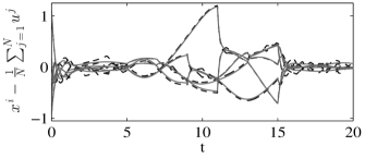
(a)

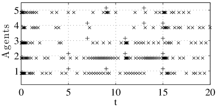
(b)

Figure 1: Executions of (4) with the event-triggered communication law described in Section 3 whose sampling rule is (11) and of (2) with continuous-time communication. The network is a weight-balanced time-varying digraph of $5$ agents with unit weights, where for $t\in[0,5)$ it is a fixed ring digraph, for $t\in[5,15)$ every $2$ seconds it is a single connected pair of nodes and then for $t\in[15,\infty)$ it is a ring digraph again. The inputs are $u^{1}(t)\!=\!0.5\sin(0.8t)$, $u^{2}(t)\!=\!0.5\sin(0.7t)\!+\!0.5\cos(0.6t)$, $u^{3}(t)=\sin(0.2t)\!+\!1$, $u^{4}(t)\!=\!\text{atan}(0.5t)$, $u^{5}(t)\!=\!0.1\cos(2t)$. The top plot shows the tracking error and the bottom one shows the communication times of each agent. Black dashed (resp. gray solid) lines correspond to the event-triggered strategy with the sampling law (11) with $\epsilon_{i}\!=\!0.1$ (resp. continuous-time communication (2)). In both cases, $\alpha\!=\!1$ and $\beta\!=\!4$. For each agent, $\times$ indicates a sampling (and broadcast) time and $+$ indicates a time when the agent acquires a new in-neighbor.

5 Simulations

In this section, we illustrate the performance of the coordination algorithm (4) under the event-triggered communication laws (11) and (22) over a recurrently jointly strongly connected digraph (cf. Fig. 1), a ring graph (cf. Fig. 2) and a time-varying connected graph (cf. Fig. 3). Figure 1 shows a small degradation between the tracking performance of the algorithm (4) with the event-triggered communication law (11) and the algorithm (2) with continuous-time communication. In the event-triggered implementation, the number of times that agents $\{1,2,3,4,5\}$ communicate in the time interval $[0,20]$ is $(41,49,44,31,40)$, respectively. The large error observed in the time interval $[5,15)$ is expected as in this time period every two seconds only two agents are communicating with each other. Naturally, these two agents tend to converge to the average of their inputs and the rest of the agents, being oblivious to the inputs of the other agents, follow their own input.

Figure 2 compares the algorithm (4) with event-triggered communication (22) and the Euler discretizations of the algorithm (2) and the proportional-integral (PI) dynamic average consensus algorithm proposed in [Freeman et al., 2006]. We set the parameters of the PI algorithm so that its ultimate tracking error is similar to that of (2). For the discretizations, we use the largest possible fixed stepsize $\delta=0.039$ for the PI algorithm (beyond this value the algorithm diverges) and we use the stepsize $\delta=0.12$ for the algorithm (2) (from [Kia et al., 2014b], convergence is guaranteed if $\delta\in(0,\min\{\alpha^{-1},\beta^{-1}(\text{d}_{\max}^{\text{out}})^{-1}\})$, which for this example results in $\delta\in(0,0.125)$). The number of times that agents $\{1,2,3,4,5\}$ communicate in the time interval $[0,20]$ is $(39,40,42,40,39)$, respectively, when implementing event-triggered communication (22). This is significantly less than the communication used by each agent in the Euler discretizations of (2) ($20/0.12\simeq 166$ rounds) and the PI algorithm ($20/0.039\simeq 512$ rounds).

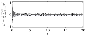
(a)

(b)

(c)

Figure 2: Comparison between the algorithm (4) employing the event-triggered communication law described in Section 3 with sampling rule (22) and the Euler discretizations of the algorithm (2) and the proportional-integral (PI) dynamic average consensus algorithm proposed in [Freeman et al., 2006]. For the first two, we set $\alpha=1$ and $\beta=4$. For the latter, we set $\gamma=5$, $\boldsymbol{\mathbf{L}}_{\text{P}}=\boldsymbol{\mathbf{L}}$ and $\boldsymbol{\mathbf{L}}_{\text{I}}=4\boldsymbol{\mathbf{L}}$. The network is a connected ring graph of $5$ agents with unit weights and the inputs are the same of Figure 1. In the top plot, black (resp. gray) lines correspond to the event-triggered law (22) with $\epsilon_{i}/(2\sqrt{\mathsf{d}_{\operatorname{out}}^{i}})=0.1$ (resp. the Euler discretization of the algorithm (2) with fixed stepsize $\delta=0.12$). The middle plot shows the response of the Euler discretization of the PI algorithm with fixed stepsize $\delta=0.039$. The horizontal lines in both the top and middle plots show the $\pm 0.05$ error bound for reference. The bottom plot shows the communication times of each agent using the event-triggered strategy.

Figure 3 shows the execution of (4) with the event-triggered communication laws (11) and (22) over a time-varying connected graph. For each agent $i\in\{1,2,3,4,5\}$, we choose $\epsilon_{i}$ for each law so that the summand in the right-hand side of the trigger ($\epsilon_{i}$ for (11), $\epsilon_{i}/(2\sqrt{\bar{\mathsf{d}}_{\operatorname{out}}^{i}})$ for (22)) amounts to the same quantity. The plots show similar tracking performance for both algorithms, with the law (22) inducing less than half communication than (11). In fact, the number of times that agents $\{1,2,3,4,5\}$ communicate in the time interval $[0,12]$ is $(43,56,72,57,55)$ under (11) and $(21,30,33,26,23)$ under (22).

(a)

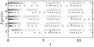
(b)

Figure 3: Executions of (4) with the sampling rule (11) and (22) with the event-triggered communication law described in Section 3. The network is a time-varying graph of $5$ agents corresponding to a connected ring graph with unit weights where one edge breaks every 3 seconds. The inputs are $u^{1}(t)\!=\!0.5\sin(t)+1/(t+2)+2$, $u^{2}(t)\!=\!0.5\sin(t)+1/(t+2)^{2}+4$, $u^{3}(t)\!=\!0.5\sin(t)+1/(t+2)^{3}+5$, $u^{4}(t)\!=\!0.5\sin(t)+\text{e}^{-t}+4$, $u^{5}(t)\!=\!0.5\sin(t)+\text{atan}(t)-1.5$. The top plot shows the tracking error with the gray solid (resp. black dashed) lines correspond to the law (11) with $\epsilon_{i}\!=\!0.1$ (resp. (22) with $\epsilon_{i}/(2\sqrt{\mathsf{d}_{\operatorname{out}}^{i}})\!=\!0.1$). In both cases, $\alpha=\beta=1$. The bottom plot shows the communication times of each agent with o (resp. $\times$) markers corresponding to the law (11) (resp. (22)). For both cases, $+$ shows the broadcasts associated to the acquisition of new in-neighbors.

6 Conclusions

We have studied the multi-agent dynamic average consensus problem over networks where inter-agent communication takes place at discrete time instants in an opportunistic fashion. Our starting point has been our previously developed continuous-time dynamic average consensus algorithm which is known to converge exponentially to a small neighborhood of the network’s inputs average. We have proposed two different distributed event-triggered laws that agents can employ to trigger communication with neighbors, depending on whether the interaction topology is described by a weight-balanced and recurrently jointly strongly connected digraph or a time-varying connected undirected graph. In both cases, we have established the correctness of the algorithm and showed that a positive lower bound on the inter-event times of each agent exists, ruling out the presence of Zeno behavior. Future work will be devoted to further relaxing the connectivity requirements on the interaction topology (tying them in to the evolution of the dynamic inputs available to the agents), the improvement of the practical convergence guarantees using time-varying thresholds in the trigger design, the use of agent abstractions in the development of self-triggered communication laws, and the synthesis of other distributed triggers that individual agents can evaluate autonomously and lead to a more efficient use of the limited network resources.

References

• Bai et al. [2010] H. Bai, R. A. Freeman, and K. M. Lynch. Robust dynamic average consensus of time-varying inputs. In IEEE Int. Conf. on Decision and Control, pages 3104–3109, Atlanta, GA, USA, December 2010.
• Bullo et al. [2009] F. Bullo, J. Cortés, and S. Martínez. Distributed Control of Robotic Networks. Applied Mathematics Series. Princeton University Press, 2009. ISBN 978-0-691-14195-4. Available at http://www.coordinationbook.info.
• Carron et al. [2013] A. Carron, M. Todescato, R. Carli, and L. Schenato. Adaptive consensus-based algorithms for fast estimation from relative measurements. In IFAC Workshop on Distributed Estimation and Control in Networked Systems, Koblenz, Germany, March 2013.
• Dimarogonas et al. [2012] D. V. Dimarogonas, E. Frazzoli, and K. H. Johansson. Distributed event-triggered control for multi-agent systems. IEEE Transactions on Automatic Control, 57(5):1291–1297, 2012.
• Donkers and Heemels [2012] M. C. F. Donkers and W. P. M. H. Heemels. Output-based event-triggered control with guaranteed $\mathcal{L}_{\infty}$-gain and improved and decentralized event-triggering. IEEE Transactions on Automatic Control, 57(6):1362–1376, 2012.
• Fan et al. [2013] Y. Fan, G. Feng, Y Wang, and C. Song. Distributed event-triggered control of multi-agent systems with combinational measurements. Automatica, 49(2):671–675, 2013.
• Freeman et al. [2006] R. A. Freeman, P. Yang, and K. M. Lynch. Stability and convergence properties of dynamic average consensus estimators. In IEEE Int. Conf. on Decision and Control, pages 338–343, 2006.
• Garcia et al. [2013] E. Garcia, Y. Cao, H. Yuc, P. Antsaklis, and D. Casbeer. Decentralised event-triggered cooperative control with limited communication. International Journal of Control, 86(9):1479–1488, 2013.
• Heemels et al. [2012] W. P. M. H. Heemels, K.H Johansson, and P. Tabuada. An introduction to event-triggered and self-triggered control. In IEEE Int. Conf. on Decision and Control, pages 3270–3285, Maui, HI, 2012.
• Khalil [2002] H. Khalil. Nonlinear Systems. Prentice Hall, 2002.
• Kia et al. [2014a] S. S. Kia, J. Cortés, and S. Martínez. Dynamic average consensus with distributed event-triggered communication. In IEEE Int. Conf. on Decision and Control, Los Angeles, CA, 2014a. Submitted.
• Kia et al. [2014b] S. S. Kia, J. Cortés, and S. Martínez. Dynamic average consensus under limited control authority and privacy requirements. International Journal on Robust and Nonlinear Control, 2014b. To appear.
• Mazo and Tabuada [2011] M. Mazo and P. Tabuada. Decentralized event-triggered control over wireless sensor/actuator networks. IEEE Transactions on Automatic Control, 56(10):2456–2461, 2011.
• Nowzari and Cortés [2014] C. Nowzari and J. Cortés. Zeno-free, distributed event-triggered communication and control for multi-agent average consensus. In American Control Conference, Portland, OR, 2014. To appear.
• Olfati-Saber [2007] R. Olfati-Saber. Distributed Kalman filtering for sensor networks. In IEEE Int. Conf. on Decision and Control, pages 5492–5498, New Orleans, LA, December 2007.
• Olfati-Saber and Shamma [2005] R. Olfati-Saber and J. S. Shamma. Consensus filters for sensor networks and distributed sensor fusion. In IEEE Int. Conf. on Decision and Control and European Control Conference, pages 6698–6703, Seville, Spain, December 2005.
• Seyboth et al. [2013] G. S. Seyboth, D. V. Dimarogonas, and K. H. Johansson. Event-based broadcasting for multi-agent average consensus. Automatica, 49(1):245–252, 2013.
• Spanos et al. [2005] D. P. Spanos, R. Olfati-Saber, and R. M. Murray. Dynamic consensus on mobile networks. In IFAC World Congress, Prague, Czech Republic, July 2005.
• Wang and Lemmon [2011] X. Wang and M. D. Lemmon. Event-triggering in distributed networked control systems. IEEE Transactions on Automatic Control, 56(3):586–601, 2011.
• Yang et al. [2007] P. Yang, R. A. Freeman, and K. M. Lynch. Distributed cooperative active sensing using consensus filters. In IEEE Int. Conf. on Robotics and Automation, pages 405–410, Roma, Italy, April 2007.
• Yang et al. [2008] P. Yang, R. A. Freeman, and K. M. Lynch. Multi-agent coordination by decentralized estimation and control. IEEE Transactions on Automatic Control, 53(11):2480?–2496, 2008.
• Zhu and Martínez [2010] M. Zhu and S. Martínez. Discrete-time dynamic average consensus. Automatica, 46(2):322–329, 2010.