Abstract

Existence of the upper critical dimension $d_{c2}=4$ for the Anderson transition is a rigorous consequence of the Bogoliubov theorem on renormalizability of $\phi^{4}$ theory. For dimensions $d\geq 4$, one-parameter scaling does not hold, and all existent numerical data should be reinterpreted. These data are exhausted by results for $d=4,\,5$ from scaling in quasi-one-dimensional systems, and results for $d=4,\,5,\,6$ from level statistics. All these data are compatible with the theoretical scaling dependencies obtained from self-consistent theory of localization by Vollhardt and W${\rm{\ddot{o}}}$lfle. The critical discussion is given for a widespread point of view that $d_{c2}=\infty$.

The main defect of the current literature on the Anderson transition is the ignorance of the upper critical dimension $d_{c2}=4$, which is a rigorous consequence of the Bogoliubov theorem on renormalizability of $\phi^{4}$ theory [1, 2]. The problem of the Anderson transition can be reduced (in the mathematically exact manner) to one of the variants of $\phi^{4}$ theory [3, 4, 5, 6] , which is nonrenormalizable for space dimensions $d>4$. Therefore, the cut-off momentum $\Lambda$, corresponding to the atomic length scale $a$, cannot be excluded from results. It rules out the existence of one-parameter scaling [9], according to which the correlation radius $\xi$ is the only essential length scale. In the latter case, any dimensionless quantity $Q$, related to a finite system of size $L$, can be written as a function of ratio $L/\xi$,

$$Q=F(L/\xi)\,,$$

which is a base for all numerical algorithms. The study of $Q$ as a function of $L$ and a distance to the transition $\tau$ allows to determine the critical exponent $\nu$ of the correlation length ($\xi\sim|\tau|^{-\nu}$). Indeed, if two $L$-dependencies for $\tau=\tau_{1}$ and $\tau=\tau_{2}$ are calculated, then the scale transformation allows to determine the ratio of two correlation lengths. Producing this procedure for a succession $\tau_{1}$, $\tau_{2}$ $\tau_{3},\,\ldots$, one can determine $\xi(\tau_{i})$ apart from numerical factor.

Relation (1) is invalid for $d>4$, and the more general form should be used,

$$Q=F(L/\xi,L/a)\,.$$

For $d=4$, a situation is more complicated and needs the additional study; in fact, the existence of logarithmic factors like $\ln(L/a)$ leads to the relation of type (2). The latter can be reduced to a function of one argument, if an appropriate choice of the scaling variables is made [10, 11].

Currently, there exist the following results for the Anderson transition in high dimensions: the data by Markos for $d=4$, $d=5$ [12, 13], obtained from scaling in quasi-one-dimensional systems; the data by Zharekeshev and Kramer for $d=4$ [14], and those by Garcia-Garcia and Cuevas for $d=5$, $d=6$ [15], obtained from the level statistics. All these results are based on relation (1) and need reinterpretation due to above arguments.

Below (Secs. 3, 4) these results are compared with the modified scaling for high dimensions obtained in [10, 11] from self-consistent theory of localization by Vollhardt and W${\rm{\ddot{o}}}$lfle [17]. The latter gives correct values of the upper critical dimension $d_{c2}=4$ and the exponent $\nu=1/2$ for $d>d_{c2}$, and at least is of interest as a possible scenario. According to certain arguments [18, 19], the Vollhardt and W${\rm{\ddot{o}}}$lfle theory predicts the exact critical behavior, and a lot of numerical results can be matched with it [10, 11, 20, 21]. The present paper supports the same tendency: all indicated numerical data [13, 14, 15] can be matched with theoretical scaling dependencies. As a rule, the ”experimental” points lie on the quasi-linear portions of the scaling curves, and was interpreted as dependence $L^{1/\nu}$ with $\nu\approx 1$ in the original papers. The actual critical behavior suggests $\nu=1/2$, but the corresponding parts of the scaling dependencies are difficult for study in numerical experiments due to their restricted accuracy.

The widespread viewpoint that $d_{c2}=\infty$ [22]–[27], is discussed in the next section.

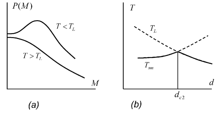
Figure 1: (a) One can use the sigma-model concept only in the case when the distribution function $P(M)$ of the modulus of ${\bf M}$ has a maximum at finite $M$. Such a maximum arises as a result of the mean-field type transition in the spirit of the Landau theory. (b) The temperature $T_{L}$ at which a sigma-model arises and the critical point $T_{sm}$ according to the ”sigma-model scenario” as functions of space dimensionality $d$. Solid and dashed lines show the real and fictitious phase transitions.

2. Sigma-models and $d_{c2}$.

A hypothesis that $d_{c2}=\infty$ is based on the following arguments:

(a) In the approach based on the use of the sigma-models [16], there are no indications on existence of the special dimensionality in the interval $2<d<\infty$ [22].

(b) Results $s=\infty$, $\nu=1/2$ for $d=\infty$ [23, 24] ($s$ is the critical exponent of conductivity) show validity of the Wegner relation $s=\nu(d-2)$ for $d=\infty$, and one can expect that this relation (and, consequently, the one-parameter scaling picture [9]) is valid for all $d>2$.

We do not question results $s=\infty$, $\nu=1/2$ for the infinite-dimensional sigma-model, but there is a problem of their correspondence with the initial disordered system. For electrons in the random potential, derivation of sigma-models is substantiated only for dimensions $d=2+\epsilon$ with $\epsilon\ll 1$; qualitatively, it can be extended to $\epsilon\sim 1$ but not to $d\gg 1$. Extension of sigma-models to higher dimensions is based on the artificial construction corresponding to a system of weakly connected metallic granules [22]. In each granule, only the zero Fourier component of the matrix field $Q$ is taken into account, while connections between granules are supposed to produce only slow variation of $Q$. The possibility that a coupling between granules leads to induction of higher Fourier components and a practical destruction of the sigma-model is not considered, while such situation looks rather probable from a standpoint of spatially homogeneous systems .

Let explain a situation on the example of the vector sigma-model. If a ferromagnet is described in terms of $\phi^{4}$ theory, then the magnetic moment ${\bf M}$ of a finite block can be considered as the Heisenberg spin with a certain fluctuation of its modulus $M$. Neglecting of such longitudinal fluctuations (which can be rigorously justified in dimensions $d=2+\epsilon$) by definition corresponds to a sigma-model. For $d=3$, the longitudinal fluctuations have no qualitative effect and the sigma-model looks applicable . However, when $d$ approaches to 4, the longitudinal fluctuations become anomalously soft and this is the origin of the upper critical dimension. If longitudinal fluctuations are artificially suppressed (which is a case in the sigma-models), then it can lead to elimination of $d_{c2}$.

In fact, one can use the sigma-model concept only in the case, when the distribution function $P(M)$ of the modulus of ${\bf M}$ has a maximum at finite $M$ (Fig.1,a). With a decrease of temperature, such a maximum arises in the result of the mean field type transition in the spirit of the Landau theory. However, the corresponding temperature $T_{L}$ does not signify the actual phase transition, since the transverse fluctuations of ${\bf M}$ destroy the long range order. Long range correlations for the transversal fluctuations arise at the lower temperature $T_{sm}$. Therefore, with a decrease of temperature, firstly (at point $T_{L}$) a sigma-model arises, and secondly (at point $T_{sm}$) the phase transition takes place according to the ”sigma-model scenario”. One can imagine that with change of $d$, dependencies $T_{L}(d)$ and $T_{sm}(d)$ intersect at point $d_{c2}$ (Fig.1,b). Hence, for $d>d_{c2}$ the phase transition occurs at the same point $T_{L}$ where a sigma-model arises, i.e. according to the ”Landau scenario”.

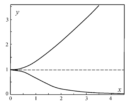
Figure 2: Scaling function $y(x)$, corresponding to high dimensions, for an algorithm based on the use of the auxiliary quasi-one-dimensional systems.

One can see that the ”sigma-model transition” (at point $T_{sm}$) is not realized for $d>d_{c2}$, if the properties of the sigma-model correspond to the properties of the real system. However, such transition can exist (as a theoretical construction) and correspond to the analytical continuation from lower dimensions, if a sigma-model is introduced artificially. In our opinion, exactly such situation takes place in the Anderson transition theory: the results $s=\infty$, $\nu=1/2$ for $d=\infty$ correspond to the formal sigma-model and not to the initial disordered system . Direct analysis of the Bete lattice (without use of sigma-models) gives results $s=1$, $\nu=1/2$ [30, 31], in correspondence with the Vollhardt and W${\rm{\ddot{o}}}$lfle theory.

In addition, let discuss the paper [27] where a conclusion that $d_{c2}=\infty$ is drawn from the modification of self-consistent theory. This paper is based on the wrong idea that the $L$ dependence for the diffusion constant in the critical point, $D_{L}\sim L^{2-d}$, signifies the existence of the momentum dependence $D(q)\sim q^{d-2}$. In fact, the dependence on $L$ arises not only from spatial, but also from the temporal dispersion, and for a given function $D(\omega,q)$ is determined by relation

$$D_{L}\sim D\left(D_{L}/L^{2},L^{-1}\right)\,.$$

If a power law dependence on $\omega$ and $q$ is accepted, then a combination

$$D(\omega,q)\sim\omega^{\eta/d}q^{d-2-\eta}$$

provides the correct behavior $D_{L}\sim L^{2-d}$ for any value of the exponent $\eta$ [32]. If one repeat the construction of [27] with an arbitrary value of $\eta$, then it is easy to test that the Wegner relation $s=\nu(d-2)$ is valid (for $d<d_{c2}$) only for $\eta=d-2$, i.e. in the absence of the spatial dispersion . For the choice $\eta=0$ made in [27], the Wegner relation is violated and the main argument of this paper (agreement with numerics) becomes fictitious, since all numerical results are based on the one-parameter scaling [9].

One of the popular numerical algorithms is based on consideration of the auxiliary quasi-one-dimensional systems [34], whose correlation length $\xi_{1D}$ is always finite. As a scaling parameter one use the quantity [12, 10]

$$z_{1}=L/\xi_{1D}\,.$$

In numerical experiments, $\xi_{1D}$ is estimated through the minimal Lyapunov exponent [34, 35], while the scaling relation of type (1) is postulated for $z_{1}$. In high dimensions such relation is invalid and one should use the modified scaling suggested in [10]. The theoretical scaling function $y(x)$ is determined by equation

$$\pm\,x^{2}=\frac{1}{y}-y^{2}\,,$$

where variables $y$ are $x$ are defined as

$$y=\frac{L}{\xi_{1D}}\left(\frac{L}{a}\right)^{(d-4)/3},\qquad x=\frac{L}{\xi}\left(\frac{L}{a}\right)^{(d-4)/3},$$

for $d>4$, and

$$y=\frac{L}{\xi_{1D}}\left[\ln(L/a)\right]^{1/3}\,,\qquad x=\frac{L}{\xi}\frac{\left[\ln(\xi/a)\right]^{1/2}}{\left[\ln(L/a)\right]^{1/6}}\,,$$

for $d=4$. Dependence $y(x)$ consists of two branches and is shown in Fig.2. It is clear from (6–8) that the usual scaling constructions are possible, if the quantity $y$ is considered as a function of the ”modified length” $\mu(L)=L^{(d-1)/3}$ ($d>4$) or $\mu(L)=L[\ln(L/a)]^{-1/6}$ ($d=4$).

Fig.3,a illustrates the numerical data by Markos for $d=4$ extracted from Fig.61 of paper [12] and presented as $z_{1}(\ln L)^{1/3}$ versus $\mu(L)$. The constant limit is realized for $W=33$, which gives the estimate of the critical point somewhat different in comparison with $W_{c}=34.3$ in [12]. Accepting $y(W,L)-y(33,L)$ as $y-y_{c}$, one can put all numerical data on the theoretical scaling curve by the change of the scale along the horizontal axis (Fig.3,b), if the common scale along the $y$ axis is chosen in appropriate manner.

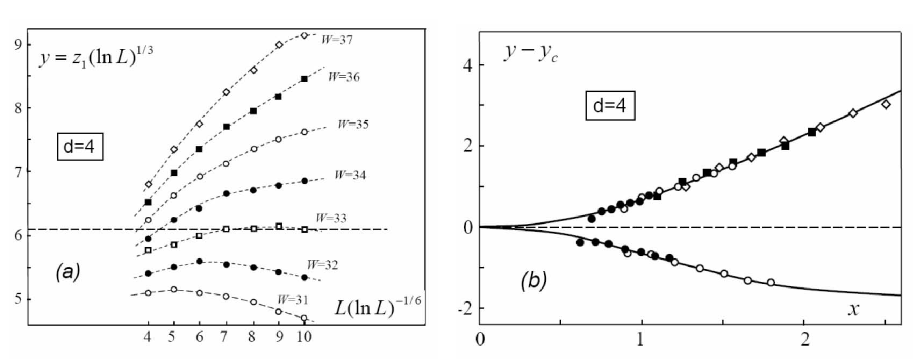
Figure 3: (a) Numerical data by Markos for $d=4$ (quasi-one-dimensional systems) extracted from Fig.61 of paper [12]; figures near the horizontal axis show the corresponding value of $L$. (b) Comparison with the theoretical scaling dependence.

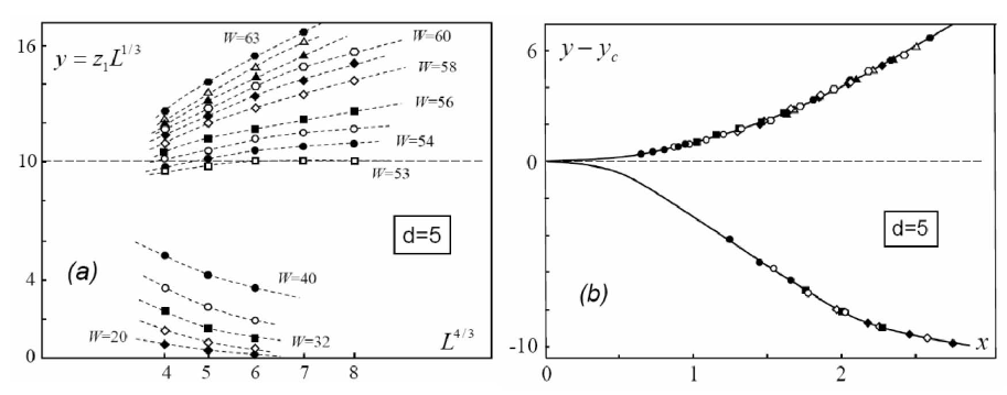
Figure 4: Numerical data by Markos for $d=5$ (quasi-one-dimensional systems) extracted from Fig.61 of paper [12] and Figs.4, 5 of paper [13] (a), and their comparison with the theoretical scaling dependence (b).

Fig.4,a illustrates the numerical data by Markos for $d=5$ extracted from Fig.61 of [12] and Figs.4,5 of [13], presented as $z_{1}L^{1/3}$ versus $L^{4/3}$. The change of the treatment procedure led to the essential shift of the critical point, from $W_{c}=57.3$ [12] to $W_{c}=53$, and made it close to the estimate $W_{c}=51.4$ of paper [15], obtained from the level statistics (see Sec. 4). Accepting $y(W,L)-y(53,L)$ as $y-y_{c}$, one can put all experimental points on the theoretical scaling curve (Fig.4,b).

In both cases, the main body of data lies on quasi-linear portions $y\sim x$ of the scaling curves and corresponds to dependencies $z_{1}\sim L(\ln L)^{1/3}$ for $d=4$ and $z_{1}\sim L$ for $d=5$, which were interpreted in [12] as $z_{1}\sim L^{1/\nu}$ with $\nu\approx 1$. In fact, these data are consistent with predictions of the Vollhardt and W${\rm{\ddot{o}}}$lfle theory, which gives $\nu=1/2$; the corresponding dependence $y-y_{c}\sim x^{2}$ is valid only for small deviations from the critical point, which are comparable with the scattering of experimental points.

To conclude the section, let discuss the technical moment related with a choice of the scaling procedure. The scaling constructions can be carried out in the usual or logarithmic coordinates, which is absolutely identical in the case of the rigorous scaling. In the actual situation, the logarithmic scaling may not provide a sufficiently smooth matching of two ”pieces” of the measured dependence, since it rigidly fix the origin of the $L$ axis. Scaling in the usual coordinates allows a more smooth matching of pieces due to small shifts along the horizontal axis. Such shifts should be absent in the case of exact scaling, but practically they arise due to scaling corrections. For example, the structure of scaling corrections to relation (1) has a following form for small $\tau$ [10]

$$y-y_{c}=\tau\left\{A_{0}L^{1/\nu}+A_{1}L^{\omega_{1}}+A_{2}L^{\omega_{2}}+\ldots\right\}+$$

$$+\left\{B_{1}L^{-\alpha_{1}}+B_{2}L^{-\alpha_{2}}+\ldots\right\}\,,$$

where $1/\nu>\omega_{1}>\omega_{2}>\ldots$, $\alpha_{1}<\alpha_{2}<\ldots$. In the accepted interpretation of $y-y_{c}$ as $y(W,L)-y(W_{c},L)$, the term in the second brackets is excluded from consideration. The expression in the first brackets is dominated by $L^{1/\nu}$ for large $L$, while other terms are dominant for small $L$: effectively, it shifts the origin of the $L$ axis. With variable $L/\xi$ used instead of $L$, such shift becomes $\tau$-dependent. If numerical data are sufficiently detailed to provide matching of pieces from the smoothness condition, then such procedure allows to account for the main scaling corrections. By this reason we use the usual and not logarithmic coordinates.

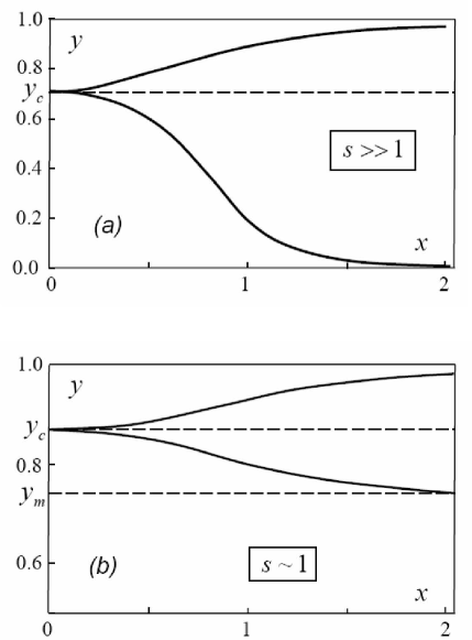
Figure 5: Examples of scaling dependencies $y(x)$ for level statistics in high dimensions: (a) for $s\gg 1$ ($u_{0}=0$) and (b) for $s\sim 1$ ($u_{0}=22.3$). The choice of parameters $k_{1}=0.0652$, $B=0.230$ corresponds to numerical data for $d=4$ [11].

4. Level statistics.

In the analysis of level statistics [11], the following combination is of the main interest,

$$y=\sigma^{2}/\sigma_{P}^{2}\,,$$

where $\sigma$ is a root-mean-square fluctuation of the number of levels $N$ in the energy interval $E=s\Delta$, where $\Delta$ is the mean level spacing in a finite system, and $\sigma_{P}$ is a value of $\sigma$ for the Poisson statistics. This quantity is closely related with parameter $A$ in the asymptotics of the distribution function $P(s)$

$$P(s)\sim\exp\left(-As\right)\,,\qquad A=\sigma_{P}^{2}/\sigma^{2}$$

of the distance $\omega=s\Delta$ between the nearest levels in the large $s$ limit. According to [11], the quantity (10) is a function of variable $x$, which is defined as

$$x=s^{-1/4}\,\frac{L}{\xi}\left(\frac{L}{a}\right)^{(d-4)/4},\qquad d>4\,,$$

$$x=s^{-1/4}\,\frac{L}{\xi}\frac{\left[\ln(\xi/a)\right]^{1/2}}{\left[\ln(L/a)\right]^{1/4}},\qquad d=4\,.$$

Dependence $y(x)$ in the parametric form is given by equations

$$y=\frac{\sigma^{2}}{\sigma_{P}^{2}}=k_{1}u\ln\frac{1+k_{1}+k_{1}u}{k_{1}+k_{1}u}\,,$$

$$\pm\,x^{2}=\frac{(1+u)^{1/2}-B(u-u_{0})}{(u-u_{0})^{1/2}}\,,$$

where the running variable $u$ changes from $u_{0}$ till infinity. Parameters $B$ and $k_{1}$ are chosen according to the procedure described in [11]; parameter $u_{0}$ account for a finiteness of $s$ and disappears for $s\to\infty$. The form of equations (14) is the same for all $d\geq 4$, while the choice of parameters depends on $d$.

Practically, the following quantity is used as a scaling variable [14]

$$J_{0}={\textstyle\frac{1}{2}}\langle s^{2}\rangle={\textstyle\frac{1}{2}}\int_{0}^{\infty}s^{2}P(s)\,ds\,,$$

or another quantity $\eta$ [15], closely related with it:

$$\eta=\frac{J_{0}-J_{0W}}{J_{0P}-J_{0W}}=\frac{J_{0}-0.643}{0.357}\,,$$

where indices $W$ and $P$ mark the values of $J_{0}$ for the Wigner–Dyson and Poisson statistics, $J_{0W}=0.643$, $J_{0P}=1$.

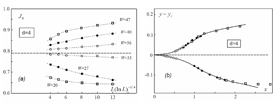
Figure 6: (a) Numerical data by Zharekeshev and Kramer for $d=4$ (level statistics), extracted from Fig.4 of paper [14] and presented as a functional dependence on the ”modified length” $\mu(L)=L(\ln L)^{-1/4}$; (b) their comparison with the theoretical scaling dependence (Fig.5,b).

Quantities $J_{0}$ and $\eta$ are the regular functions of variable (10) for some $s\sim 1$ [11], so their small deviations from the critical values are proportional to each other:

$$J_{0}-J_{0c}\sim\eta-\eta_{c}\sim y-y_{c}\,.$$

Examples of dependencies $y(x)$ for $s\to\infty$ (a) and $s\sim 1$ (b) are presented in Fig.5; they correspond to the critical value $A_{c}=1.4$ of parameter $A$ in (11), which is specific for $d=4$ [14]. Parameter $u_{0}$ in Fig.5,b is chosen so as to provide the approximate symmetry of two branches, discovered in numerical experiments by Zharekeshev and Kramer [14] (Fig.6,a). These data can be successfully matched with the theoretical dependence (Fig.6,b).

The critical value $y_{c}$ (Fig.5,a) tends to unity with the increase of $d$. Indeed, starting from the critical values $A_{c}=1.4$ ($d=4$) [14], $A_{c}=1.17$ ($d=5$) [15], $A_{c}=1.13$ ($d=6$) [15] and following the procedure of paper [11], one can obtain $y_{c}=0.714$ ($d=4$), $y_{c}=0.858$ ($d=5$), $y_{c}=0.885$ ($d=6$). This tendency agrees with the theorem [35], that level statistics for the Bete lattice (corresponding to $d=\infty$) has the Poisson form even in the metallic phase.

With this observation, it is possible to obtain the universal scaling function for high dimensions. Suggesting $1-y\ll 1$, one can expand the first equation (14) in $1/k_{1}u$ and linearize the right hand side of the second equation (14) near the critical value $u_{c}$; then

$$y-y_{c}={\rm const}\,F(x)\,,\qquad F(x)=\frac{\pm x^{2}}{1\pm x^{2}}\,,$$

where an appropriate choice of the common scale along the $x$ axis is made; signs $+$ and $-$ corresponds to the upper and lower branches of function $F(x)$ shown in Fig.7; singularity at $x=1$ is fictitious and lies beyond the limits of applicability of (18). According to (17), deviations of $J_{0}$ and $\eta$ from the critical values are described by the same function.

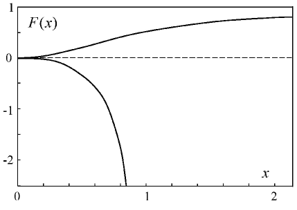
Figure 7: The universal scaling dependence for level statistics, corresponding to high dimensions.

Fig.8,a and Fig.9,a illustrates the numerical data by Garcia–Garcia and Cuevas [15] for $d=5$ and $d=6$ presented as a functional dependence on the ”modified length” $\mu(L)=L^{d/4}$; they are in a good agreement with the universal scaling function $F(x)$ (see Fig.8,b and Fig.9,b).

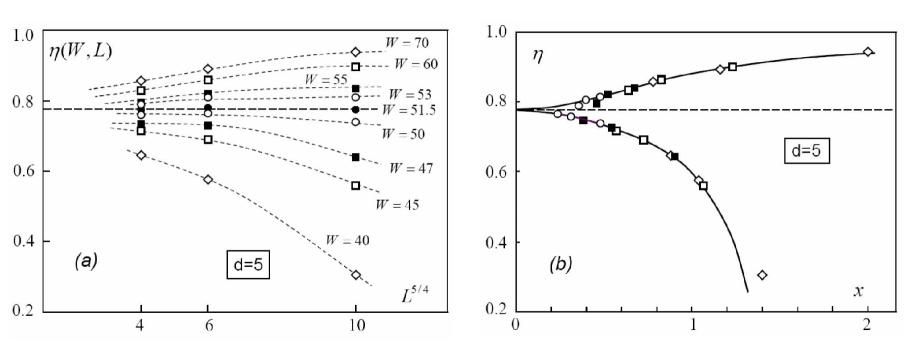
Figure 8: Numerical data by Garcia–Garcia and Cuevas for $d=5$ (level statistics), extracted from Fig.1 of paper [15] (a) and their comparison with the theoretical scaling dependence shown in Fig.7 (b).

In cases $d=5$ and $d=6$ (in opposite to $d=4$) corrections related with a finiteness of $s$ are not essential. Indeed, according to [14] the quantity $J_{0}$ at $d=4$ runs the interval $(0.64,0.79)$ along the lower branch, and the interval $(0.79,1.00)$ along the upper branch. According to [15], these intervals are $(0.64,0.92)$, $(0.92,1.00)$ for $d=5$, and $(0.64,0.95)$, $(0.95,1.00)$ for $d=6$. If a choice of $u_{0}$ provides the same proportion for the intervals $(y_{m},y_{c})$ and $(y_{c},1)$ in Fig.5,b, then $1-y_{c}\approx y_{c}-y_{m}$ for $d=4$ and $1-y_{c}\ll y_{c}-y_{m}$ for $d=5,\,6$. In the latter case, the difference of $y_{m}$ from zero is practically not manifested in the region of applicability for (18).

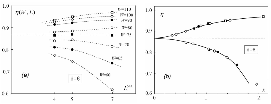
Figure 9: Numerical data by Garcia–Garcia and Cuevas for $d=6$ (level statistics), extracted from Fig.1 of paper [15] (a) and their comparison with the universal scaling dependence (b).

For $d>4$, equations (14) define scaling of the form

$$y=\frac{\sigma^{2}}{\sigma_{P}^{2}}=F\left(\frac{L^{d/4}}{\xi a^{(d-4)/4}}\right)\,,$$

which for large $\xi$ gives

$$y=\tilde{F}\left(\tau\frac{L^{d/4\,\nu}}{a^{(d-4)/4\,\nu}}\right)=y_{c}+C\tau L^{d/4\,\nu}+\ldots\,,$$

i.e. derivative $y^{\prime}_{\tau}$ at $\tau=0$ has a behavior $L^{d/4\,\nu}$ instead $L^{1/\nu}$ corresponding to scaling of type (1). Hence, values of the exponents $\nu=0.84$ ($d=5$), $\nu=0.78$ ($d=6$) obtained in [15] in the framework of (1) transform to $\nu=0.67$ ($d=5$), $\nu=0.52$ ($d=6$) if (19) is used. Therefore, the results of paper [15] for $d=5,\,6$ becomes close to $\nu=1/2$ simply in the result of transfer to a correct scaling relation. Situation for $d=4$ is analogous to that of Sec. 3, i. e. the main body of data corresponds to quasi-linear portions $y\sim x\sim L(\ln L)^{-1/4}$ of the scaling curves, which was interpreted in [14, 15] as $L^{1/\nu}$ with $\nu\approx 1$. Such situation is aggravated by the accepted scheme of treatment when a derivative over $\tau=W-W_{c}$ is determined by expansion over $W-W_{c}$ and fitting by a polynomial of finite degree. In such procedure, the result is dominated by experimental points remote of $W_{c}$ and linearity in $x$ preserves even in case, when the data close to $W_{c}$ demonstrate an essential nonlinearity.

5. Conclusion

The present paper suggests a new interpretation of existing numerical data for the Anderson transition in high dimensions: results for $d=4,\,5$ obtained from scaling in quasi-one-dimensional systems, and results for $d=4,\,5,\,6$ obtained from level statistics. Such reinterpretation is necessary due to the absence of one-parameter scaling [9] in high dimensions, which is a consequence of nonrenormalizability of theory. All indicated numerical data appear to be compatible with theoretical scaling dependencies obtained from self-consistent theory of localization by Vollhardt and W${\rm{\ddot{o}}}$lfle. It supports the same tendency as was observed in preceding papers [10, 11, 20, 21]: on the level of raw data, the Vollhardt and W${\rm{\ddot{o}}}$lfle theory looks satisfactory, while the opposite statements of the original papers are related with ambiguity of the treatment procedure. It gives new arguments in favor of the viewpoint [18, 19] that the Vollhardt and W${\rm{\ddot{o}}}$lfle theory predicts the exact critical behavior.

References

- [1] N. N. Bogoliubov and D. V. Shirkov, Introduction to the Theory of Quantized Fields (Nauka, Moscow, 1976; Wiley, New York, 1980).
- [2] E. Brezin, J. C. Le Guillou, J. Zinn-Justin, in Phase Transitions and Critical Phenomena, ed. by C. Domb and M. S. Green, Academic, New York (1976), Vol. VI.
- [3] S. Ma, Modern Theory of Critical Phenomena (Benjamin, Reading, Mass., 1976).
- [4] A. Nitzan, K. F. Freed, M. N. Cohen, Phys. Rev. B 15, 4476 (1977).
- [5] M. V. Sadovskii, Usp. Fiz. Nauk 133, 223 (1981) [Sov. Phys. Usp. 24, 96 (1981)];
- [6] I. M. Suslov, Usp. Fiz. Nauk 168, 503 (1998) [Physics – Uspekhi 41, 441 (1998)].
- [7] J. J. M. Verbaarschot, M. R. Zirnbauer, J. Phys. A 18, 1093 (1985).
- [8] M. R. Zirnbauer, cond-mat/9903338.
- [9] E. Abrahams, P. W. Anderson, D. C. Licciardello, and T. V. Ramakrishman, Phys. Rev. Lett. 42, 673 (1979).
- [10] I. M. Suslov, Zh. Eksp. Teor. Fiz. 141, 122 (2012) [ JETP 114, 107 (2012)].
- [11] I. M. Suslov, Zh. Eksp. Teor. Fiz. 145, issue 5 (2014); arXiv: 1402.2382.
- [12] P. Markos, acta physica slovaca 56, 561 (2006); cond-mat/0609580.
- [13] P. Markos, Zh. Eksp. Teor. Fiz. 142, 1226 (2012) [ JETP 115, 1075 (2012)].
- [14] I. Kh. Zharekeshev, B. Kramer, Ann. Phys. (Leipzig) 7, 442 (1998).
- [15] A. M. Garcia-Garcia, E. Cuevas, Phys. Rev. B 75, 174203 (2007).
- [16] F. Wegner, Z. Phys. B 35, 207 (1979); L. Schfer, F. Wegner, Z. Phys. B 38, 113 (1980). S. Hikami, Phys. Rev. B 24, 2671 (1981). K. B. Efetov, A. I. Larkin, D. E. Khmelnitskii, Zh. Eksp. Teor. Fiz. 79, 1120 (1980) [Sov. Phys. JETP 52, 568 (1980)]. K. B. Efetov, Adv. Phys. 32, 53 (1983).
- [17] D. Vollhardt, P. Wlfle, Phys. Rev. B 22, 4666 (1980); Phys. Rev. Lett. 48, 699 (1982). D. Vollhardt, P. Wlfle, in Modern Problems in Condensed Matter Sciences, ed. by V. M. Agranovich and A. A. Maradudin, v. 32, North-Holland, Amsterdam (1992).
- [18] H. Kunz, R. Souillard, J. de Phys. Lett. 44, L506 (1983).
- [19] I. M. Suslov, Zh. Eksp. Teor. Fiz. 108, 1686 (1995) [ JETP 81, 925 (1995)].
- [20] I. M. Suslov, Zh. Eksp. Teor. Fiz. 142, 1020 (2012) [ JETP 115, 897 (2012)].
- [21] I. M. Suslov, Zh. Eksp. Teor. Fiz. 142, 1230 (2012) [ JETP 115, 1079 (2012)].
- [22] K. B. Efetov, Zh. Eksp. Teor. Fiz. 88, 1032 (1985) [Sov. Phys. JETP 61, 606 (1985)].
- [23] K. B. Efetov, Zh. Eksp. Teor. Fiz. 93, 1125 (1987); 94, 357 (1988) [Sov. Phys. JETP 66, 634 (1987); 67, 199 (1988)].
- [24] M. R. Zirnbauer, Phys. Rev. B 34, 6394 (1986); Nucl. Phys. B 265, 375 (1986).
- [25] A. D. Mirlin, Y. V. Fyodorov, Phys. Rev. Lett. 72, 526 (1994).
- [26] F. Evers, A. D. Mirlin, Rev. Mod. Phys. 80, 1355 (2008).
- [27] A. M. Garcia-Garcia, Phys. Rev. Lett. 100, 076404 (2008).
- [28] K. B. Efetov, Zh. Eksp. Teor. Fiz. 83, 833 (1982) [Sov. Phys. JETP 56, 467 (1982)].
- [29] M. Moshe, J. Zinn-Justin, Phys. Rept. 385, 69 (2003).
- [30] B. Shapiro, Phys. Rev. Lett. 50, 747 (1983).
- [31] H. Kunz, R. Souillard, J. de Phys. Lett. 44, L411 (1983).
- [32] J. T. Chalker, Physica A 167, 253 (1990). T. Brandes, B. Huckestein, L. Schweitzer, Ann. Phys. 5, 633 (1996).
- [33] I. M. Suslov, cond-mat/0612654.
- [34] J. L. Pichard, G. Sarma, J. Phys. C: Solid State Phys. 14, L127 (1981).
- [35] A. MacKinnon, B. Kramer, Phys. Rev. Lett. 47, 1546 (1981).
- [36] M. Aizenman, S. Warzel, Math. Phys. Anal. Geom. 9, 291 (2006).