Generalized Nonconvex Nonsmooth Low-Rank Minimization

Canyi Lu1, Jinhui Tang2, Shuicheng Yan1, Zhouchen Lin3,
1 Department of Electrical and Computer Engineering, National University of Singapore
2 School of Computer Science, Nanjing University of Science and Technology
3 Key Laboratory of Machine Perception (MOE), School of EECS, Peking University
canyilu@gmail.com, jinhuitang@mail.njust.edu.cn, eleyans@nus.edu.sg, zlin@pku.edu.cn
Corresponding author.
Abstract

As surrogate functions of L0subscript𝐿0L_{0}-norm, many nonconvex penalty functions have been proposed to enhance the sparse vector recovery. It is easy to extend these nonconvex penalty functions on singular values of a matrix to enhance low-rank matrix recovery. However, different from convex optimization, solving the nonconvex low-rank minimization problem is much more challenging than the nonconvex sparse minimization problem. We observe that all the existing nonconvex penalty functions are concave and monotonically increasing on [0,)0[0,\infty). Thus their gradients are decreasing functions. Based on this property, we propose an Iteratively Reweighted Nuclear Norm (IRNN) algorithm to solve the nonconvex nonsmooth low-rank minimization problem. IRNN iteratively solves a Weighted Singular Value Thresholding (WSVT) problem. By setting the weight vector as the gradient of the concave penalty function, the WSVT problem has a closed form solution. In theory, we prove that IRNN decreases the objective function value monotonically, and any limit point is a stationary point. Extensive experiments on both synthetic data and real images demonstrate that IRNN enhances the low-rank matrix recovery compared with state-of-the-art convex algorithms.
Refer to caption
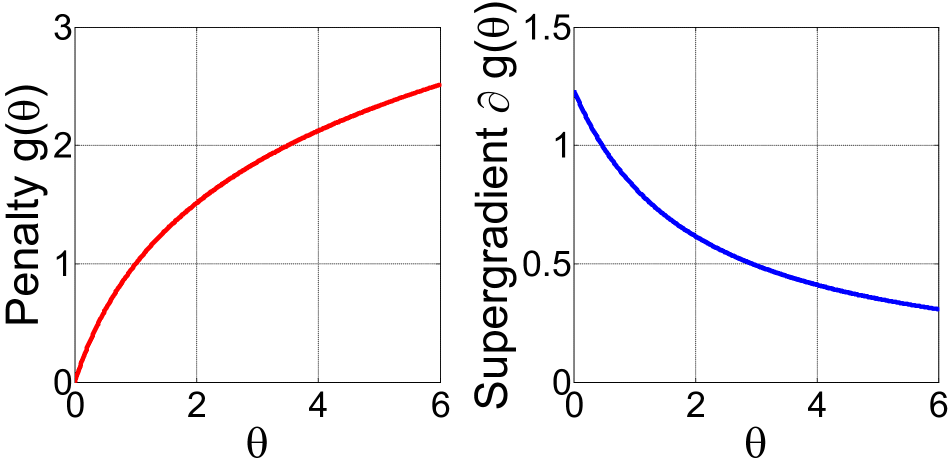
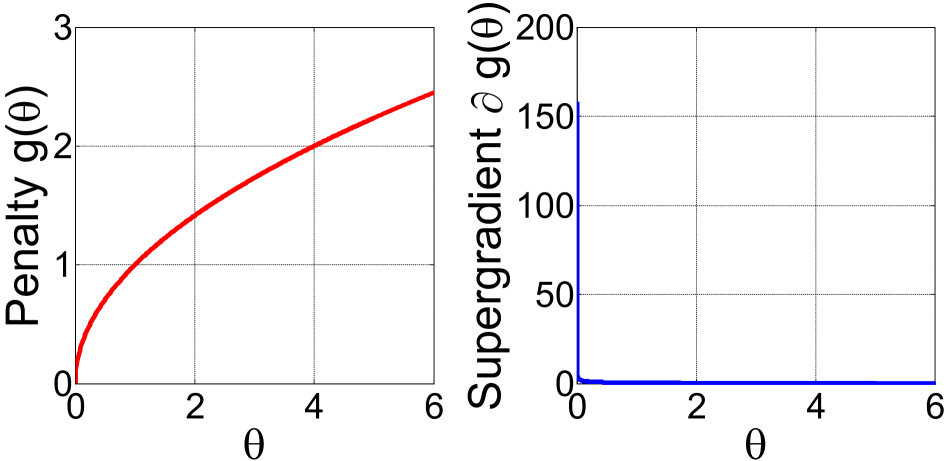
(a) Lpsubscript𝐿𝑝L_{p} Penalty [11]
Refer to caption
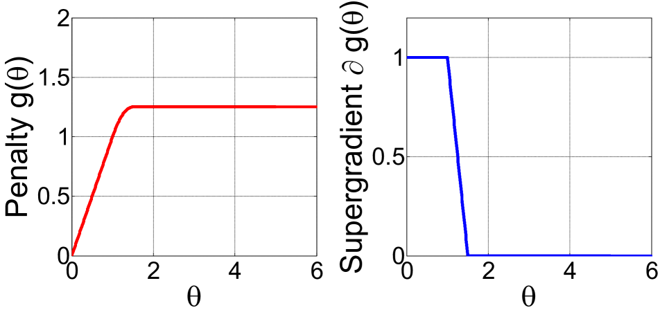
(b) SCAD Penalty [10]
Refer to caption
(c) Logarithm Penalty [12]
Refer to caption
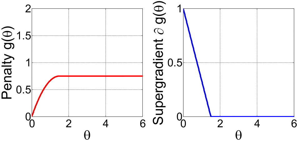
(d) MCP Penalty [23]
Refer to caption
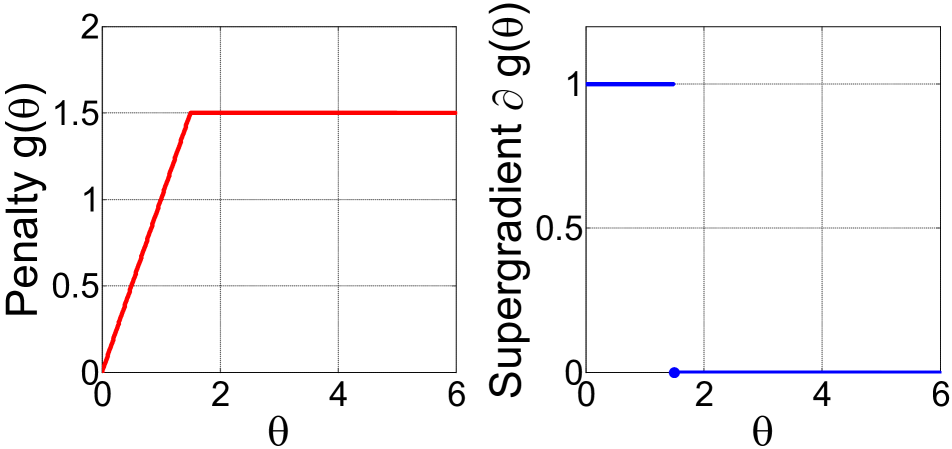
(e) Capped L1subscript𝐿1L_{1} Penalty [24]
Refer to caption
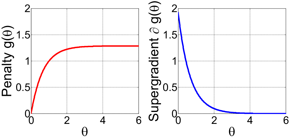
(f) ETP Penalty [13]
Refer to caption
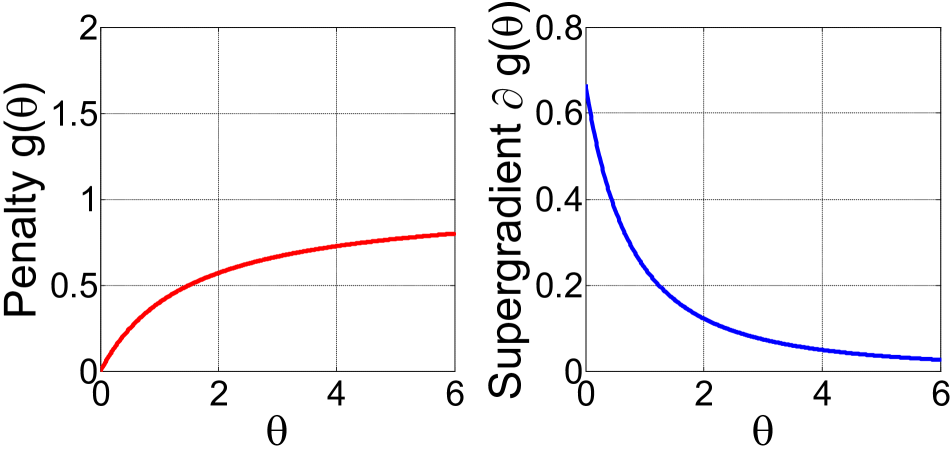
(g) Geman Penalty [15]
Refer to caption
(h) Laplace Penalty [21]
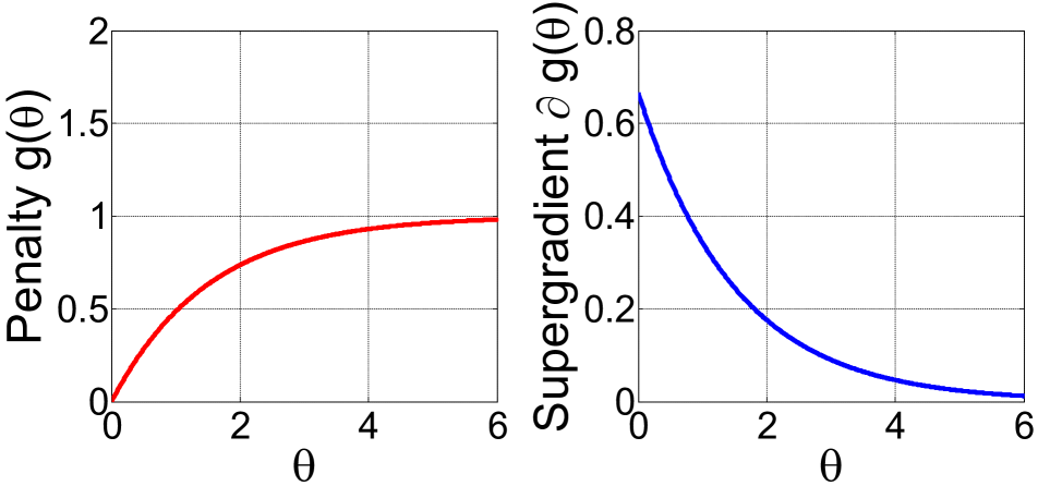
Figure 1: Illustration of the popular nonconvex surrogate functions of θ0subscriptnorm𝜃0||\theta||_{0} (left), and their supergradients (right). All these penalty functions share the common properties: concave and monotonically increasing on [0,)0[0,\infty). Thus their supergradients (see Section 2.1) are nonnegative and monotonically decreasing. Our proposed general solver is based on this key observation.
Table 1: Popular nonconvex surrogate functions of θ0subscriptnorm𝜃0||\theta||_{0} and their supergradients.
Penalty Formula gλ(θ)subscript𝑔𝜆𝜃g_{\lambda}(\theta), θ0𝜃0\theta\geq 0, λ>0𝜆0\lambda>0 Supergradient gλ(θ)subscript𝑔𝜆𝜃\partial g_{\lambda}(\theta)
Lpsubscript𝐿𝑝L_{p} [11] λθp𝜆superscript𝜃𝑝\lambda\theta^{p} {, if θ=0,λpθp1, if θ>0.cases if 𝜃0𝜆𝑝superscript𝜃𝑝1 if 𝜃0\begin{cases}\infty,&\text{ if }\theta=0,\\ \lambda p\theta^{p-1},&\text{ if }\theta>0.\end{cases}
SCAD [10] {λθ, if θλ,θ2+2γλθλ22(γ1), if λ<θγλ,λ2(γ+1)2, if θ>γλ.cases𝜆𝜃 if 𝜃𝜆superscript𝜃22𝛾𝜆𝜃superscript𝜆22𝛾1 if 𝜆𝜃𝛾𝜆superscript𝜆2𝛾12 if 𝜃𝛾𝜆\begin{cases}\lambda\theta,&\text{ if }\theta\leq\lambda,\\ \frac{-\theta^{2}+2\gamma\lambda\theta-\lambda^{2}}{2(\gamma-1)},&\text{ if }\lambda<\theta\leq\gamma\lambda,\\ \frac{\lambda^{2}(\gamma+1)}{2},&\text{ if }\theta>\gamma\lambda.\end{cases} {λ, if θλ,γλθγ1, if λ<θγλ,0, if θ>γλ.cases𝜆 if 𝜃𝜆𝛾𝜆𝜃𝛾1 if 𝜆𝜃𝛾𝜆0 if 𝜃𝛾𝜆\begin{cases}\lambda,&\text{ if }\theta\leq\lambda,\\ \frac{\gamma\lambda-\theta}{\gamma-1},&\text{ if }\lambda<\theta\leq\gamma\lambda,\\ 0,&\text{ if }\theta>\gamma\lambda.\end{cases}
Logarithm [12] λlog(γ+1)log(γθ+1)𝜆𝛾1𝛾𝜃1\frac{\lambda}{\log(\gamma+1)}\log(\gamma\theta+1) γλ(γθ+1)log(γ+1)𝛾𝜆𝛾𝜃1𝛾1\frac{\gamma\lambda}{(\gamma\theta+1)\log(\gamma+1)}
MCP [23] {λθθ22γ, if θ<γλ,12γλ2, if θγλ.cases𝜆𝜃superscript𝜃22𝛾 if 𝜃𝛾𝜆12𝛾superscript𝜆2 if 𝜃𝛾𝜆\begin{cases}\lambda\theta-\frac{\theta^{2}}{2\gamma},&\text{ if }\theta<\gamma\lambda,\\ \frac{1}{2}\gamma\lambda^{2},&\text{ if }\theta\geq\gamma\lambda.\end{cases} {λθγ, if θ<γλ,0, if θγλ.cases𝜆𝜃𝛾 if 𝜃𝛾𝜆0 if 𝜃𝛾𝜆\begin{cases}\lambda-\frac{\theta}{\gamma},&\text{ if }\theta<\gamma\lambda,\\ 0,&\text{ if }\theta\geq\gamma\lambda.\end{cases}
Capped L1subscript𝐿1L_{1} [24] {λθ, if θ<γ,λγ, if θγ.cases𝜆𝜃 if 𝜃𝛾𝜆𝛾 if 𝜃𝛾\begin{cases}\lambda\theta,&\text{ if }\theta<\gamma,\\ \lambda\gamma,&\text{ if }\theta\geq\gamma.\end{cases} {λ, if θ<γ,[0,λ], if θ=γ,0, if θ>γ.cases𝜆 if 𝜃𝛾0𝜆 if 𝜃𝛾0 if 𝜃𝛾\begin{cases}\lambda,&\text{ if }\theta<\gamma,\\ [0,\lambda],&\text{ if }\theta=\gamma,\\ 0,&\text{ if }\theta>\gamma.\end{cases}
ETP [13] λ1exp(γ)(1exp(γθ))𝜆1𝛾1𝛾𝜃\frac{\lambda}{1-\exp(-\gamma)}(1-\exp(-\gamma\theta)) λγ1exp(γ)exp(γθ)𝜆𝛾1𝛾𝛾𝜃\frac{\lambda\gamma}{1-\exp(-\gamma)}\exp(-\gamma\theta)
Geman [15] λθθ+γ𝜆𝜃𝜃𝛾\frac{\lambda\theta}{\theta+\gamma} λγ(θ+γ)2𝜆𝛾superscript𝜃𝛾2\frac{\lambda\gamma}{(\theta+\gamma)^{2}}
Laplace [21] λ(1exp(θγ))𝜆1𝜃𝛾\lambda(1-\exp(-\frac{\theta}{\gamma})) λγexp(θγ)𝜆𝛾𝜃𝛾\frac{\lambda}{\gamma}\exp(-\frac{\theta}{\gamma})

1 Introduction

This paper aims to solve the following general nonconvex nonsmooth low-rank minimization problem

min𝐗m×nF(𝐗)=i=1mgλ(σi(𝐗))+f(𝐗),subscript𝐗superscript𝑚𝑛𝐹𝐗superscriptsubscript𝑖1𝑚subscript𝑔𝜆subscript𝜎𝑖𝐗𝑓𝐗\min_{\mathbf{X}\in\mathbb{R}^{m\times n}}F(\operatorname*{\mathbf{X}})=\sum_{i=1}^{m}g_{\lambda}(\sigma_{i}(\mathbf{X}))+f(\mathbf{X}), (1)

where σi(𝐗)subscript𝜎𝑖𝐗\sigma_{i}(\operatorname*{\mathbf{X}}) denotes the i𝑖i-th singular value of 𝐗m×n𝐗superscript𝑚𝑛\operatorname*{\mathbf{X}}\in\mathbb{R}^{m\times n} (we assume mn𝑚𝑛m\leq n in this work). The penalty function gλsubscript𝑔𝜆g_{\lambda} and loss function f𝑓f satisfy the following assumptions:

  • A1

    gλ::subscript𝑔𝜆absentg_{\lambda}: +superscript\mathbb{R}\rightarrow\mathbb{R}^{+} is continuous, concave and monotonically increasing on [0,)0[0,\infty). It is possibly nonsmooth.

  • A2

    f𝑓f: m×n+superscript𝑚𝑛superscript\mathbb{R}^{m\times n}\rightarrow\mathbb{R}^{+} is a smooth function of type C1,1superscript𝐶11C^{1,1}, i.e., the gradient is Lipschitz continuous,

    f(𝐗)f(𝐘)FL(f)𝐗𝐘F,subscriptnorm𝑓𝐗𝑓𝐘𝐹𝐿𝑓subscriptnorm𝐗𝐘𝐹||\nabla f(\mathbf{X})-\nabla f(\mathbf{Y})||_{F}\leq L(f)||\mathbf{X}-\mathbf{Y}||_{F}, (2)

    for any 𝐗,𝐘m×n𝐗𝐘superscript𝑚𝑛\mathbf{X},\mathbf{Y}\in\mathbb{R}^{m\times n}, L(f)>0𝐿𝑓0L(f)>0 is called Lipschitz constant of f𝑓\nabla f. f(𝐗)𝑓𝐗f(\operatorname*{\mathbf{X}}) is possibly nonconvex.

  • A3

    F(𝐗)𝐹𝐗F(\operatorname*{\mathbf{X}})\rightarrow\infty iff 𝐗Fsubscriptnorm𝐗𝐹||\operatorname*{\mathbf{X}}||_{F}\rightarrow\infty.

Many optimization problems in machine learning and computer vision areas fall into the formulation in (1). As for the choice of f𝑓f, the squared loss f(𝐗)=12𝒜(𝐗)𝐛F2𝑓𝐗12superscriptsubscriptnorm𝒜𝐗𝐛𝐹2f(\operatorname*{\mathbf{X}})=\frac{1}{2}||\mathcal{A}(\operatorname*{\mathbf{X}})-\mathbf{b}||_{F}^{2}, with a linear mapping 𝒜𝒜\mathcal{A}, is widely used. In this case, the Lipschitz constant of f𝑓\nabla f is then the spectral radius of 𝒜𝒜superscript𝒜𝒜\mathcal{A}^{*}\mathcal{A}, i.e., L(f)=ρ(𝒜𝒜)𝐿𝑓𝜌superscript𝒜𝒜L(f)=\rho(\mathcal{A}^{*}\mathcal{A}), where 𝒜superscript𝒜\mathcal{A}^{*} is the adjoint operator of 𝒜𝒜\mathcal{A}. By choosing gλ(x)=λxsubscript𝑔𝜆𝑥𝜆𝑥g_{\lambda}(x)=\lambda x, i=1mgλ(σi(𝐗))superscriptsubscript𝑖1𝑚subscript𝑔𝜆subscript𝜎𝑖𝐗\sum_{i=1}^{m}g_{\lambda}(\sigma_{i}(\operatorname*{\mathbf{X}})) is exactly the nuclear norm λi=1mσi(𝐗)=λ𝐗𝜆superscriptsubscript𝑖1𝑚subscript𝜎𝑖𝐗𝜆subscriptnorm𝐗\lambda\sum_{i=1}^{m}\sigma_{i}(\operatorname*{\mathbf{X}})=\lambda||\operatorname*{\mathbf{X}}||_{*}. Problem (1) resorts to the well known nuclear norm regularized problem

min𝐗λ𝐗+f(𝐗).subscript𝐗𝜆subscriptnorm𝐗𝑓𝐗\min_{\operatorname*{\mathbf{X}}}\lambda||\operatorname*{\mathbf{X}}||_{*}+f(\operatorname*{\mathbf{X}}). (3)

If f(𝐗)𝑓𝐗f(\operatorname*{\mathbf{X}}) is convex, it is the most widely used convex relaxation of the rank minimization problem:

min𝐗λrank(𝐗)+f(𝐗).subscript𝐗𝜆rank𝐗𝑓𝐗\min_{\operatorname*{\mathbf{X}}}\lambda\text{rank}(\operatorname*{\mathbf{X}})+f(\operatorname*{\mathbf{X}}). (4)

The above low-rank minimization problem arises in many machine learning tasks such as multiple category classification [1], matrix completion [20], multi-task learning [2], and low-rank representation with squared loss for subspace segmentation [18]. However, solving problem (4) is usually difficult, or even NP-hard. Most previous works solve the convex problem (3) instead. It has been proved that under certain incoherence assumptions on the singular values of the matrix, solving the convex nuclear norm regularized problem leads to a near optimal low-rank solution [6]. However, such assumptions may be violated in real applications. The obtained solution by using nuclear norm may be suboptimal since it is not a perfect approximation of the rank function. A similar phenomenon has been observed in the convex L1subscript𝐿1L_{1}-norm and nonconvex L0subscript𝐿0L_{0}-norm for sparse vector recovery [7].

In order to achieve a better approximation of the L0subscript𝐿0L_{0}-norm, many nonconvex surrogate functions of L0subscript𝐿0L_{0}-norm have been proposed, including Lpsubscript𝐿𝑝L_{p}-norm [11], Smoothly Clipped Absolute Deviation (SCAD) [10], Logarithm [12], Minimax Concave Penalty (MCP) [23], Capped L1subscript𝐿1L_{1} [24], Exponential-Type Penalty (ETP) [13], Geman [15], and Laplace [21]. Table 1 tabulates these penalty functions and Figure 1 visualizes them. One may refer to [14] for more properties of these penalty functions. Some of these nonconvex penalties have been extended to approximate the rank function, e.g. the Schatten-p𝑝p norm [19]. Another nonconvex surrogate of rank function is the truncated nuclear norm [16].

For nonconvex sparse minimization, several algorithms have been proposed to solve the problem with a nonconvex regularizer. A common method is DC (Difference of Convex functions) programming [14]. It minimizes the nonconvex function f(𝐱)(gλ(𝐱))𝑓𝐱subscript𝑔𝜆𝐱f(\operatorname*{\mathbf{x}})-(-g_{\lambda}(\operatorname*{\mathbf{x}})) based on the assumption that both f𝑓f and gλsubscript𝑔𝜆-g_{\lambda} are convex. In each iteration, DC programming linearizes gλ(𝐱)subscript𝑔𝜆𝐱-g_{\lambda}(\operatorname*{\mathbf{x}}) at 𝐱=𝐱k𝐱superscript𝐱𝑘\operatorname*{\mathbf{x}}={\operatorname*{\mathbf{x}}}^{k}, and minimizes the relaxed function as follows

𝐱k+1=argmin𝐱f(𝐱)(gλ(𝐱k))𝐯k,𝐱𝐱k,superscript𝐱𝑘1subscript𝐱𝑓𝐱subscript𝑔𝜆superscript𝐱𝑘superscript𝐯𝑘𝐱superscript𝐱𝑘{\operatorname*{\mathbf{x}}}^{k+1}=\arg\min_{\operatorname*{\mathbf{x}}}f(\operatorname*{\mathbf{x}})-(-g_{\lambda}({\operatorname*{\mathbf{x}}}^{k}))-\left\langle\mathbf{v}^{k},\operatorname*{\mathbf{x}}-{\operatorname*{\mathbf{x}}}^{k}\right\rangle, (5)

where 𝐯ksuperscript𝐯𝑘{\mathbf{v}}^{k} is a subgradient of gλ(𝐱)subscript𝑔𝜆𝐱-g_{\lambda}(\operatorname*{\mathbf{x}}) at 𝐱=𝐱k𝐱subscript𝐱𝑘\operatorname*{\mathbf{x}}=\operatorname*{\mathbf{x}}_{k}. DC programming may be not very efficient, since it requires some other iterative algorithm to solve (5). Note that the updating rule (5) of DC programming cannot be extended to solve the low-rank problem (1). The reason is that for concave gλsubscript𝑔𝜆g_{\lambda}, i=1mgλ(σi(𝐗))superscriptsubscript𝑖1𝑚subscript𝑔𝜆subscript𝜎𝑖𝐗-\sum_{i=1}^{m}g_{\lambda}(\sigma_{i}(\operatorname*{\mathbf{X}})) does not guarantee to be convex w.r.t. 𝐗𝐗\operatorname*{\mathbf{X}}. DC programming also fails when f𝑓f is nonconvex in problem (1).

Another solver is to use the proximal gradient algorithm which is originally designed for convex problem [3]. It requires computing the proximal operator of gλsubscript𝑔𝜆g_{\lambda},

Pgλ(y)=argminxgλ(x)+12(xy)2,subscript𝑃subscript𝑔𝜆𝑦subscript𝑥subscript𝑔𝜆𝑥12superscript𝑥𝑦2P_{g_{\lambda}}(y)=\arg\min_{x}g_{\lambda}(x)+\frac{1}{2}(x-y)^{2}, (6)

in each iteration. However, for nonconvex gλsubscript𝑔𝜆g_{\lambda}, there may not exist a general solver for (6). Even if (6) is solvable, different from convex optimization, (Pgλ(y1)Pgλ(y2))(y1y2)0subscript𝑃subscript𝑔𝜆subscript𝑦1subscript𝑃subscript𝑔𝜆subscript𝑦2subscript𝑦1subscript𝑦20(P_{g_{\lambda}}(y_{1})-P_{g_{\lambda}}(y_{2}))(y_{1}-y_{2})\geq 0 does not always hold. Thus we cannot perform Pgλ()subscript𝑃subscript𝑔𝜆P_{g_{\lambda}}(\cdot) on the singular values of 𝐘𝐘\operatorname*{\mathbf{Y}} directly for solving

Pgλ(𝐘)=argmin𝐗i=1mgλ(σi(𝐗))+𝐗𝐘F2.subscript𝑃subscript𝑔𝜆𝐘subscript𝐗superscriptsubscript𝑖1𝑚subscript𝑔𝜆subscript𝜎𝑖𝐗superscriptsubscriptnorm𝐗𝐘𝐹2P_{g_{\lambda}}(\operatorname*{\mathbf{Y}})=\arg\min_{\operatorname*{\mathbf{X}}}\sum_{i=1}^{m}g_{\lambda}(\sigma_{i}(\operatorname*{\mathbf{X}}))+||\operatorname*{\mathbf{X}}-\operatorname*{\mathbf{Y}}||_{F}^{2}. (7)

The nonconvexity of gλsubscript𝑔𝜆g_{\lambda} makes the nonconvex low-rank minimization problem much more challenging than the nonconvex sparse minimization.

Another related work is the Iteratively Reweighted Least Squares (IRLS) algorihtm. It has been recently extended to handle the nonconvex Schatten-p𝑝p norm penalty [19]. Actually it solves a relaxed smooth problem which may require many iterations to achieve a low-rank solution. It cannot solve the general nonsmooth problem (1). The alternative updating algorithm in [16] minimizes the truncated nuclear norm by using a special property of this penalty. It contains two loops, both of which require computing SVD. Thus it is not very efficient. It cannot be extended to solve the general problem (1) either.

In this work, all the existing nonconvex surrogate functions of L0subscript𝐿0L_{0}-norm are extended on the singular values of a matrix to enhance low-rank recovery. In problem (1), gλsubscript𝑔𝜆g_{\lambda} can be any existing nonconvex penalty function shown in Table 1 or any other function which satisfies the assumption (A1). We observe that all the existing nonconvex surrogate functions are concave and monotonically increasing on [0,)0[0,\infty). Thus their gradients (or supergradients at the nonsmooth points) are nonnegative and monotonically decreasing. Based on this key fact, we propose an Iteratively Reweighted Nuclear Norm (IRNN) algorithm to solve problem (1). IRNN computes the proximal operator of the weighted nuclear norm, which has a closed form solution due to the nonnegative and monotonically decreasing supergradients. In theory, we prove that IRNN monotonically decreases the objective function value, and any limit point is a stationary point. To the best of our knowledge, IRNN is the first work which is able to solve the general problem (1) with convergence guarantee. Note that for nonconvex optmization, it is usually very difficult to prove that an algorithm converges to stationary points. At last, we test our algorithm with several nonconvex penalty functions on both synthetic data and real image data to show the effectiveness of the proposed algorithm.

Refer to caption
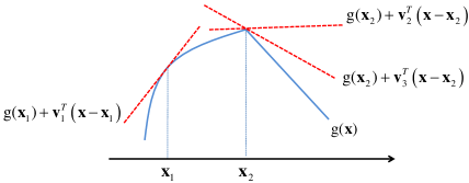
Figure 2: Supergraidients of a concave function. 𝐯1subscript𝐯1\mathbf{v}_{1} is a supergradient at 𝐱1subscript𝐱1\mathbf{x}_{1}, and 𝐯2subscript𝐯2\mathbf{v}_{2} and 𝐯3subscript𝐯3\mathbf{v}_{3} are supergradients at 𝐱2subscript𝐱2\mathbf{x}_{2}.

2 Nonconvex Nonsmooth Low-Rank Minimization

In this section, we present a general algorithm to solve problem (1). To handle the case that gλsubscript𝑔𝜆g_{\lambda} is nonsmooth, e.g., Capped L1subscript𝐿1L_{1} penalty, we need the concept of supergradient defined on the concave function.

2.1 Supergradient of a Concave Function

The subgradient of the convex function is an extension of gradient at a nonsmooth point. Similarly, the supergradient is an extension of gradient of the concave function at a nonsmooth point. If g(𝐱)𝑔𝐱g(\operatorname*{\mathbf{x}}) is concave and differentiable at 𝐱𝐱\operatorname*{\mathbf{x}}, it is known that

g(𝐱)+g(𝐱),𝐲𝐱g(𝐲).𝑔𝐱𝑔𝐱𝐲𝐱𝑔𝐲g(\operatorname*{\mathbf{x}})+\langle\nabla g(\operatorname*{\mathbf{x}}),\operatorname*{\mathbf{y}}-\operatorname*{\mathbf{x}}\rangle\geq g(\operatorname*{\mathbf{y}}). (8)

If g(𝐱)𝑔𝐱g(\operatorname*{\mathbf{x}}) is nonsmooth at 𝐱𝐱\operatorname*{\mathbf{x}}, the supergradient extends the gradient at 𝐱𝐱\operatorname*{\mathbf{x}} inspired by (8) [5].

Definition 1

Let g:n:𝑔superscript𝑛g:\mathbb{R}^{n}\rightarrow\mathbb{R} be concave. A vector 𝐯𝐯\mathbf{v} is a supergradient of g𝑔g at the point 𝐱n𝐱superscript𝑛\operatorname*{\mathbf{x}}\in\mathbb{R}^{n} if for every 𝐲n𝐲superscript𝑛\operatorname*{\mathbf{y}}\in\mathbb{R}^{n}, the following inequality holds

g(𝐱)+𝐯,𝐲𝐱g(𝐲).𝑔𝐱𝐯𝐲𝐱𝑔𝐲g(\operatorname*{\mathbf{x}})+\langle\mathbf{v},\operatorname*{\mathbf{y}}-\operatorname*{\mathbf{x}}\rangle\geq g(\operatorname*{\mathbf{y}}). (9)

All supergradients of g𝑔g at 𝐱𝐱\operatorname*{\mathbf{x}} are called the superdifferential of g𝑔g at 𝐱𝐱\operatorname*{\mathbf{x}}, and are denoted as g(𝐱)𝑔𝐱\partial g(\operatorname*{\mathbf{x}}). If g𝑔g is differentiable at 𝐱𝐱\operatorname*{\mathbf{x}}, g(𝐱)𝑔𝐱\nabla g(\operatorname*{\mathbf{x}}) is also a supergradient, i.e., g(𝐱)={g(𝐱)}𝑔𝐱𝑔𝐱\partial g(\operatorname*{\mathbf{x}})=\{\nabla g(\operatorname*{\mathbf{x}})\}. Figure 2 illustrates the supergradients of a concave function at both differentiable and nondifferentiable points.

For concave g𝑔g, g𝑔-g is convex, and vice versa. From this fact, we have the following relationship between the supergradient of g𝑔g and the subgradient of g𝑔-g.

Lemma 1

Let g(𝐱)𝑔𝐱g(\operatorname*{\mathbf{x}}) be concave and h(𝐱)=g(𝐱)𝐱𝑔𝐱h(\operatorname*{\mathbf{x}})=-g(\operatorname*{\mathbf{x}}). For any 𝐯g(𝐱)𝐯𝑔𝐱\mathbf{v}\in\partial g(\operatorname*{\mathbf{x}}), 𝐮=𝐯h(𝐱)𝐮𝐯𝐱\mathbf{u}=-\mathbf{v}\in\partial h(\operatorname*{\mathbf{x}}), and vice versa.

The relationship of the supergradient and subgradient shown in Lemma 1 is useful for exploring some properties of the supergradient. It is known that the subdiffierential of a convex function hh is a monotone operator, i.e.,

𝐮𝐯,𝐱𝐲0,𝐮𝐯𝐱𝐲0\langle\mathbf{u}-\mathbf{v},\operatorname*{\mathbf{x}}-\operatorname*{\mathbf{y}}\rangle\geq 0, (10)

for any 𝐮h(𝐱)𝐮𝐱\mathbf{u}\in\partial h(\operatorname*{\mathbf{x}}), 𝐯h(𝐲)𝐯𝐲\mathbf{v}\in\partial h(\operatorname*{\mathbf{y}}). The superdifferential of a concave function holds a similar property, which is called antimonotone operator in this work.

Lemma 2

The superdifferential of a concave function g𝑔g is an antimonotone operator, i.e.,

𝐮𝐯,𝐱𝐲0,𝐮𝐯𝐱𝐲0\langle\mathbf{u}-\mathbf{v},\operatorname*{\mathbf{x}}-\operatorname*{\mathbf{y}}\rangle\leq 0, (11)

for any 𝐮g(𝐱)𝐮𝑔𝐱\mathbf{u}\in\partial g(\operatorname*{\mathbf{x}}), 𝐯g(𝐲)𝐯𝑔𝐲\mathbf{v}\in\partial g(\operatorname*{\mathbf{y}}).

This can be easily proved by Lemma 1 and (10).

Lemma 2 is a key lemma in this work. Supposing that the assumption (A1) holds for g(x)𝑔𝑥g(x), (11) indicates that

uv, for any ug(x) and vg(y),formulae-sequence𝑢𝑣 for any 𝑢𝑔𝑥 and 𝑣𝑔𝑦u\geq v,\text{ for any }u\in\partial g(x)\text{ and }v\in\partial g(y), (12)

when xy𝑥𝑦x\leq y. That is to say, the supergradient of g𝑔g is monotonically decreasing on [0,)0[0,\infty). Table 1 shows some usual concave functions and their supergradients. We also visualize them in Figure 1. It can be seen that they all satisfy the assumption (A1). Note that for the Lpsubscript𝐿𝑝L_{p} penalty, we further define that g(0)=𝑔0\partial g(0)=\infty. This will not affect our algorithm and convergence analysis as shown latter. The Capped L1subscript𝐿1L_{1} penalty is nonsmooth at θ=γ𝜃𝛾\theta=\gamma, with the superdifferential gλ(γ)=[0,λ]subscript𝑔𝜆𝛾0𝜆\partial g_{\lambda}(\gamma)=[0,\lambda].

2.2 Iteratively Reweighted Nuclear Norm

In this subsection, we show how to solve the general nonconvex and possibly nonsmooth problem (1) based on the assumptions (A1)-(A2). For simplicity of notation, we denote σi=σi(𝐗)subscript𝜎𝑖subscript𝜎𝑖𝐗\sigma_{i}=\sigma_{i}(\operatorname*{\mathbf{X}}) and σik=σi(𝐗k)superscriptsubscript𝜎𝑖𝑘subscript𝜎𝑖superscript𝐗𝑘\sigma_{i}^{k}=\sigma_{i}(\operatorname*{\mathbf{X}}^{k}).

Since gλsubscript𝑔𝜆g_{\lambda} is concave on [0,)0[0,\infty), by the definition of the supergradient, we have

gλ(σi)gλ(σik)+wik(σiσik),subscript𝑔𝜆subscript𝜎𝑖subscript𝑔𝜆subscriptsuperscript𝜎𝑘𝑖superscriptsubscript𝑤𝑖𝑘subscript𝜎𝑖superscriptsubscript𝜎𝑖𝑘g_{\lambda}(\sigma_{i})\leq g_{\lambda}(\sigma^{k}_{i})+w_{i}^{k}(\sigma_{i}-\sigma_{i}^{k}), (13)

where

wikgλ(σik).superscriptsubscript𝑤𝑖𝑘subscript𝑔𝜆superscriptsubscript𝜎𝑖𝑘w_{i}^{k}\in\partial g_{\lambda}(\sigma_{i}^{k}). (14)

Since σ1kσ2kσmk0superscriptsubscript𝜎1𝑘superscriptsubscript𝜎2𝑘superscriptsubscript𝜎𝑚𝑘0\sigma_{1}^{k}\geq\sigma_{2}^{k}\geq\cdots\geq\sigma_{m}^{k}\geq 0, by the antimonotone property of supergradient (12), we have

0w1kw2kwmk.0superscriptsubscript𝑤1𝑘superscriptsubscript𝑤2𝑘superscriptsubscript𝑤𝑚𝑘0\leq w_{1}^{k}\leq w_{2}^{k}\leq\cdots\leq w_{m}^{k}. (15)

This property is important in our algorithm shown latter. (13) motivates us to minimize its right hand side instead of gλ(σi)subscript𝑔𝜆subscript𝜎𝑖g_{\lambda}(\sigma_{i}). Thus we may solve the following relaxed problem

𝐗k+1=argmin𝐗i=1mgλ(σik)+wik(σiσik)+f(𝐗)=argmin𝐗i=1mwikσi+f(𝐗).superscript𝐗𝑘1subscript𝐗superscriptsubscript𝑖1𝑚subscript𝑔𝜆subscriptsuperscript𝜎𝑘𝑖superscriptsubscript𝑤𝑖𝑘subscript𝜎𝑖superscriptsubscript𝜎𝑖𝑘𝑓𝐗subscript𝐗superscriptsubscript𝑖1𝑚superscriptsubscript𝑤𝑖𝑘subscript𝜎𝑖𝑓𝐗\begin{split}{\operatorname*{\mathbf{X}}}^{k+1}=&\arg\min_{\operatorname*{\mathbf{X}}}\sum_{i=1}^{m}g_{\lambda}(\sigma^{k}_{i})+w_{i}^{k}(\sigma_{i}-\sigma_{i}^{k})+f(\operatorname*{\mathbf{X}})\\ =&\arg\min_{\operatorname*{\mathbf{X}}}\sum_{i=1}^{m}w_{i}^{k}\sigma_{i}+f(\operatorname*{\mathbf{X}}).\end{split} (16)

It seems that updating 𝐗k+1superscript𝐗𝑘1{\operatorname*{\mathbf{X}}}^{k+1} by solving the above weighted nuclear norm problem (16) is an extension of the weighted L1subscript𝐿1L_{1}-norm problem in IRL1 algorithm [7] (IRL1 is a special DC programming algorithm). However, the weighted nuclear norm is nonconvex in (16) (it is convex if and only if w1kw2kwmk0superscriptsubscript𝑤1𝑘superscriptsubscript𝑤2𝑘superscriptsubscript𝑤𝑚𝑘0w_{1}^{k}\geq w_{2}^{k}\geq\cdots\geq w_{m}^{k}\geq 0 [8]), while the weighted L1subscript𝐿1L_{1}-norm is convex. Solving the nonconvex problem (16) is much more challenging than the convex weighted L1subscript𝐿1L_{1}-norm problem. In fact, it is not easier than solving the original problem (1).

Algorithm 1 Solving problem (1) by IRNN

Input: μ>L(f)𝜇𝐿𝑓\mu>L(f) - A Lipschitz constant of f(𝐗)𝑓𝐗\nabla f({\operatorname*{\mathbf{X}}}).
Initialize: k=0𝑘0k=0, 𝐗ksuperscript𝐗𝑘{\operatorname*{\mathbf{X}}}^{k}, and wiksubscriptsuperscript𝑤𝑘𝑖w^{k}_{i}, i=1,,m𝑖1𝑚i=1,\cdots,m.
Output: Xsuperscript𝑋X^{*}.
while not converge do

  1. 1.

    Update 𝐗k+1superscript𝐗𝑘1{\operatorname*{\mathbf{X}}}^{k+1} by solving problem (18).

  2. 2.

    Update the weights wik+1superscriptsubscript𝑤𝑖𝑘1w_{i}^{k+1}, i=1,,m𝑖1𝑚i=1,\cdots,m, by

    wik+1gλ(σi(𝐗k+1)).superscriptsubscript𝑤𝑖𝑘1subscript𝑔𝜆subscript𝜎𝑖superscript𝐗𝑘1w_{i}^{k+1}\in\partial g_{\lambda}\left(\sigma_{i}({\operatorname*{\mathbf{X}}}^{k+1})\right). (17)

    end while

Instead of updating 𝐗k+1superscript𝐗𝑘1{\operatorname*{\mathbf{X}}}^{k+1} by solving (16), we linearize f(𝐗)𝑓𝐗f(\operatorname*{\mathbf{X}}) at 𝐗ksuperscript𝐗𝑘{\operatorname*{\mathbf{X}}^{k}} and add a proximal term:

f(𝐗)f(𝐗k)+f(𝐗k),𝐗𝐗k+μ2𝐗𝐗kF2,𝑓𝐗𝑓superscript𝐗𝑘𝑓superscript𝐗𝑘𝐗superscript𝐗𝑘𝜇2superscriptsubscriptnorm𝐗superscript𝐗𝑘𝐹2f({\operatorname*{\mathbf{X}}})\approx f({\operatorname*{\mathbf{X}}}^{k})+\langle\nabla f({\operatorname*{\mathbf{X}}}^{k}),{\operatorname*{\mathbf{X}}}-{\operatorname*{\mathbf{X}}}^{k}\rangle+\frac{\mu}{2}||{\operatorname*{\mathbf{X}}}-{\operatorname*{\mathbf{X}}}^{k}||_{F}^{2},

where μ>L(f)𝜇𝐿𝑓\mu>L(f). Such a choice of μ𝜇\mu guarantees the convergence of our algorithm as shown latter. Then we update 𝐗k+1superscript𝐗𝑘1{\operatorname*{\mathbf{X}}}^{k+1} by solving

𝐗k+1=argmin𝐗i=1mwikσi+f(𝐗k)+f(𝐗k),𝐗𝐗k+μ2𝐗𝐗kF2=argmin𝐗i=1mwikσi+μ2𝐗(𝐗k1μf(𝐗k))F2.superscript𝐗𝑘1subscript𝐗superscriptsubscript𝑖1𝑚superscriptsubscript𝑤𝑖𝑘subscript𝜎𝑖𝑓superscript𝐗𝑘𝑓superscript𝐗𝑘𝐗superscript𝐗𝑘𝜇2superscriptsubscriptnorm𝐗superscript𝐗𝑘𝐹2subscript𝐗superscriptsubscript𝑖1𝑚superscriptsubscript𝑤𝑖𝑘subscript𝜎𝑖𝜇2superscriptsubscriptdelimited-∥∥𝐗superscript𝐗𝑘1𝜇𝑓superscript𝐗𝑘𝐹2\begin{split}{\operatorname*{\mathbf{X}}}^{k+1}=&\arg\min_{{\operatorname*{\mathbf{X}}}}\sum_{i=1}^{m}w_{i}^{k}\sigma_{i}+f({\operatorname*{\mathbf{X}}}^{k})\\ &+\langle\nabla f({\operatorname*{\mathbf{X}}}^{k}),{\operatorname*{\mathbf{X}}}-{\operatorname*{\mathbf{X}}}^{k}\rangle+\frac{\mu}{2}||{\operatorname*{\mathbf{X}}}-{\operatorname*{\mathbf{X}}}^{k}||_{F}^{2}\\ =&\arg\min_{{\operatorname*{\mathbf{X}}}}\sum_{i=1}^{m}w_{i}^{k}\sigma_{i}+\frac{\mu}{2}\left\|{\operatorname*{\mathbf{X}}}-\left({\operatorname*{\mathbf{X}}}^{k}-\frac{1}{\mu}\nabla f({\operatorname*{\mathbf{X}}}^{k})\right)\right\|_{F}^{2}.\end{split} (18)

Problem (18) is still nonconvex. Fortunately, it has a closed form solution due to (15).

Lemma 3

[8, Theorem 2.3] For any λ>0𝜆0\lambda>0, 𝐘m×n𝐘superscript𝑚𝑛{\operatorname*{\mathbf{Y}}}\in\mathbb{R}^{m\times n} and 0w1w2ws(s=min(m,n))0subscript𝑤1subscript𝑤2subscript𝑤𝑠𝑠𝑚𝑛0\leq w_{1}\leq w_{2}\leq\cdots\leq w_{s}\ (s=\min(m,n)), a globally optimal solution to the following problem

minλi=1swiσi(𝐗)+12𝐗𝐘F2,𝜆superscriptsubscript𝑖1𝑠subscript𝑤𝑖subscript𝜎𝑖𝐗12superscriptsubscriptnorm𝐗𝐘𝐹2\min\lambda\sum_{i=1}^{s}w_{i}\sigma_{i}({\operatorname*{\mathbf{X}}})+\frac{1}{2}||{\operatorname*{\mathbf{X}}}-{\operatorname*{\mathbf{Y}}}||_{F}^{2}, (19)

is given by the weighted singular value thresholding

𝐗=U𝒮λ𝒘(𝚺)𝑽T,superscript𝐗𝑈subscript𝒮𝜆𝒘𝚺superscript𝑽𝑇{\operatorname*{\mathbf{X}}}^{*}=U\mathcal{S}_{\lambda\bm{w}}(\bm{\Sigma})\bm{V}^{T}, (20)

where 𝐘=𝐔𝚺𝐕T𝐘𝐔𝚺superscript𝐕𝑇{\operatorname*{\mathbf{Y}}}=\bm{U}\bm{\Sigma}\bm{V}^{T} is the SVD of 𝐘𝐘{\operatorname*{\mathbf{Y}}}, and 𝒮λ𝐰(𝚺)=Diag{(𝚺iiλwi)+}subscript𝒮𝜆𝐰𝚺Diagsubscriptsubscript𝚺𝑖𝑖𝜆subscript𝑤𝑖\mathcal{S}_{\lambda\bm{w}}(\bm{\Sigma})=\operatorname*{Diag}\{(\bm{\Sigma}_{ii}-\lambda w_{i})_{+}\}.

It is worth mentioning that for the Lpsubscript𝐿𝑝L_{p} penalty, if σik=0superscriptsubscript𝜎𝑖𝑘0\sigma_{i}^{k}=0, wikgλ(σik)={}superscriptsubscript𝑤𝑖𝑘subscript𝑔𝜆superscriptsubscript𝜎𝑖𝑘w_{i}^{k}\in\partial g_{\lambda}(\sigma_{i}^{k})=\{\infty\}. By the updating rule of 𝐗k+1superscript𝐗𝑘1\operatorname*{\mathbf{X}}^{k+1} in (18), we have σik+1=0superscriptsubscript𝜎𝑖𝑘10\sigma_{i}^{k+1}=0. This guarantees that the rank of the sequence {𝐗k}superscript𝐗𝑘\{\operatorname*{\mathbf{X}}^{k}\} is nonincreasing.

Iteratively updating wiksuperscriptsubscript𝑤𝑖𝑘w_{i}^{k}, i=1,,m𝑖1𝑚i=1,\cdots,m, by (14) and 𝐗k+1superscript𝐗𝑘1{\operatorname*{\mathbf{X}}}^{k+1} by (18) leads to the proposed Iteratively Reweighted Nuclear Norm (IRNN) algorithm. The whole procedure of IRNN is shown in Algorithm 1. If the Lipschitz constant L(f)𝐿𝑓L(f) is not known or computable, the backtracking rule can be used to estimate μ𝜇\mu in each iteration [3].

3 Convergence Analysis

In this section, we give the convergence analysis for the IRNN algorithm. We will show that IRNN decreases the objective function value monotonically, and any limit point is a stationary point of problem (1). We first recall the following well-known and fundamental property for a smooth function in the class C1,1superscript𝐶11C^{1,1}.

Lemma 4

[4, 3] Let f:m×n:𝑓superscript𝑚𝑛f:\mathbb{R}^{m\times n}\rightarrow\mathbb{R} be a continuously differentiable function with Lipschitz continuous gradient and Lipschitz constant L(f)𝐿𝑓L(f). Then, for any 𝐗,𝐘m×n𝐗𝐘superscript𝑚𝑛{\operatorname*{\mathbf{X}}},{\operatorname*{\mathbf{Y}}}\in\mathbb{R}^{m\times n}, and μL(f)𝜇𝐿𝑓\mu\geq L(f),

f(𝐗)f(𝐘)+𝐗𝐘,f(𝐘)+μ2𝐗𝐘F2.𝑓𝐗𝑓𝐘𝐗𝐘𝑓𝐘𝜇2superscriptsubscriptnorm𝐗𝐘𝐹2f({\operatorname*{\mathbf{X}}})\leq f({\operatorname*{\mathbf{Y}}})+\langle{\operatorname*{\mathbf{X}}}-{\operatorname*{\mathbf{Y}}},\nabla f({\operatorname*{\mathbf{Y}}})\rangle+\frac{\mu}{2}||{\operatorname*{\mathbf{X}}}-{\operatorname*{\mathbf{Y}}}||_{F}^{2}. (21)
Theorem 1

Assume that gλsubscript𝑔𝜆g_{\lambda} and f𝑓f in problem (1) satisfy the assumptions (A1)-(A2). The sequence {𝐗k}superscript𝐗𝑘\{{\operatorname*{\mathbf{X}}}^{k}\} generated in Algorithm 1 satisfies the following properties:

  1. (1)

    F(𝐗k)𝐹superscript𝐗𝑘F({\operatorname*{\mathbf{X}}}^{k}) is monotonically decreasing. Indeed,

    F(𝐗k)F(𝐗k+1)μL(f)2𝐗k𝐗k+1F20;𝐹superscript𝐗𝑘𝐹superscript𝐗𝑘1𝜇𝐿𝑓2superscriptsubscriptnormsuperscript𝐗𝑘superscript𝐗𝑘1𝐹20F({\operatorname*{\mathbf{X}}}^{k})-F({\operatorname*{\mathbf{X}}}^{k+1})\geq\frac{\mu-L(f)}{2}||{\operatorname*{\mathbf{X}}}^{k}-{\operatorname*{\mathbf{X}}}^{k+1}||_{F}^{2}\geq 0;
  2. (2)

    limk(𝐗k𝐗k+1)=𝟎subscript𝑘superscript𝐗𝑘superscript𝐗𝑘10\lim\limits_{k\rightarrow\infty}({\operatorname*{\mathbf{X}}}^{k}-{\operatorname*{\mathbf{X}}}^{k+1})=\bm{0};

  3. (3)

    The sequence {𝐗k}superscript𝐗𝑘\{{\operatorname*{\mathbf{X}}}^{k}\} is bounded.

Proof. First, since 𝐗k+1superscript𝐗𝑘1{\operatorname*{\mathbf{X}}}^{k+1} is a global solution to problem (18), we get

i=1mwikσik+1+f(𝐗k),𝐗k+1𝐗k+μ2𝐗k+1𝐗kF2i=1mwikσik+f(𝐗k),𝐗k𝐗k+μ2𝐗k𝐗kF2.superscriptsubscript𝑖1𝑚superscriptsubscript𝑤𝑖𝑘superscriptsubscript𝜎𝑖𝑘1𝑓superscript𝐗𝑘superscript𝐗𝑘1superscript𝐗𝑘𝜇2subscriptsuperscriptnormsuperscript𝐗𝑘1superscript𝐗𝑘2𝐹superscriptsubscript𝑖1𝑚superscriptsubscript𝑤𝑖𝑘superscriptsubscript𝜎𝑖𝑘𝑓superscript𝐗𝑘superscript𝐗𝑘superscript𝐗𝑘𝜇2subscriptsuperscriptnormsuperscript𝐗𝑘superscript𝐗𝑘2𝐹\begin{split}&\sum_{i=1}^{m}w_{i}^{k}\sigma_{i}^{k+1}+\langle\nabla f({\operatorname*{\mathbf{X}}}^{k}),{\operatorname*{\mathbf{X}}}^{k+1}-{\operatorname*{\mathbf{X}}}^{k}\rangle+\frac{\mu}{2}||{\operatorname*{\mathbf{X}}}^{k+1}-{\operatorname*{\mathbf{X}}}^{k}||^{2}_{F}\\ \leq&\sum_{i=1}^{m}w_{i}^{k}\sigma_{i}^{k}+\langle\nabla f({\operatorname*{\mathbf{X}}}^{k}),{\operatorname*{\mathbf{X}}}^{k}-{\operatorname*{\mathbf{X}}}^{k}\rangle+\frac{\mu}{2}||{\operatorname*{\mathbf{X}}}^{k}-{\operatorname*{\mathbf{X}}}^{k}||^{2}_{F}.\end{split}

It can be rewritten as

f(𝐗k),𝐗k𝐗k+1i=1mwik(σikσik+1)+μ2𝐗k𝐗k+1F2.𝑓superscript𝐗𝑘superscript𝐗𝑘superscript𝐗𝑘1superscriptsubscript𝑖1𝑚superscriptsubscript𝑤𝑖𝑘superscriptsubscript𝜎𝑖𝑘superscriptsubscript𝜎𝑖𝑘1𝜇2superscriptsubscriptnormsuperscript𝐗𝑘superscript𝐗𝑘1𝐹2\begin{split}&\langle\nabla f({\operatorname*{\mathbf{X}}}^{k}),{\operatorname*{\mathbf{X}}}^{k}-{\operatorname*{\mathbf{X}}}^{k+1}\rangle\\ \geq&-\sum_{i=1}^{m}w_{i}^{k}(\sigma_{i}^{k}-\sigma_{i}^{k+1})+\frac{\mu}{2}||{\operatorname*{\mathbf{X}}}^{k}-{\operatorname*{\mathbf{X}}}^{k+1}||_{F}^{2}.\end{split} (22)

Second, since the gradient of f(𝐗)𝑓𝐗f({\operatorname*{\mathbf{X}}}) is Lipschitz continuous, by using Lemma 4, we have

f(𝐗k)f(𝐗k+1)f(𝐗k),𝐗k𝐗k+1L(f)2𝐗k𝐗k+1F2.𝑓superscript𝐗𝑘𝑓superscript𝐗𝑘1𝑓superscript𝐗𝑘superscript𝐗𝑘superscript𝐗𝑘1𝐿𝑓2superscriptsubscriptnormsuperscript𝐗𝑘superscript𝐗𝑘1𝐹2\begin{split}&f({\operatorname*{\mathbf{X}}}^{k})-f({\operatorname*{\mathbf{X}}}^{k+1})\\ \geq&\langle\nabla f({\operatorname*{\mathbf{X}}}^{k}),{\operatorname*{\mathbf{X}}}^{k}-{\operatorname*{\mathbf{X}}}^{k+1}\rangle-\frac{L(f)}{2}||{\operatorname*{\mathbf{X}}}^{k}-{\operatorname*{\mathbf{X}}}^{k+1}||_{F}^{2}.\end{split} (23)

Third, since wikgλ(σik)superscriptsubscript𝑤𝑖𝑘subscript𝑔𝜆superscriptsubscript𝜎𝑖𝑘w_{i}^{k}\in\partial g_{\lambda}(\sigma_{i}^{k}), by the definition of the supergradient, we have

gλ(σik)gλ(σik+1)wik(σikσik+1).subscript𝑔𝜆superscriptsubscript𝜎𝑖𝑘subscript𝑔𝜆superscriptsubscript𝜎𝑖𝑘1superscriptsubscript𝑤𝑖𝑘superscriptsubscript𝜎𝑖𝑘superscriptsubscript𝜎𝑖𝑘1g_{\lambda}(\sigma_{i}^{k})-g_{\lambda}(\sigma_{i}^{k+1})\geq w_{i}^{k}(\sigma_{i}^{k}-\sigma_{i}^{k+1}). (24)

Now, summing (22), (23) and (24) for i=1,,m𝑖1𝑚i=1,\cdots,m, together, we obtain

F(𝐗k)F(𝐗k+1)=i=1m(gλ(σik)gλ(σik+1))+f(𝐗k)f(𝐗k+1)μL(f)2𝐗k+1𝐗kF20.𝐹superscript𝐗𝑘𝐹superscript𝐗𝑘1superscriptsubscript𝑖1𝑚subscript𝑔𝜆superscriptsubscript𝜎𝑖𝑘subscript𝑔𝜆superscriptsubscript𝜎𝑖𝑘1𝑓superscript𝐗𝑘𝑓superscript𝐗𝑘1𝜇𝐿𝑓2superscriptsubscriptnormsuperscript𝐗𝑘1superscript𝐗𝑘𝐹20\begin{split}&F({\operatorname*{\mathbf{X}}}^{k})-F({\operatorname*{\mathbf{X}}}^{k+1})\\ =&\sum_{i=1}^{m}\left(g_{\lambda}(\sigma_{i}^{k})-g_{\lambda}(\sigma_{i}^{k+1})\right)+f({\operatorname*{\mathbf{X}}}^{k})-f({\operatorname*{\mathbf{X}}}^{k+1})\\ \geq&\frac{\mu-L(f)}{2}||{\operatorname*{\mathbf{X}}}^{k+1}-{\operatorname*{\mathbf{X}}}^{k}||_{F}^{2}\geq 0.\\ \end{split} (25)

Thus F(𝐗k)𝐹superscript𝐗𝑘F({\operatorname*{\mathbf{X}}}^{k}) is monotonically decreasing. Summing all the inequalities in (25) for k1𝑘1k\geq 1, we get

F(𝐗1)μL(f)2k=1𝐗k+1𝐗kF2,𝐹superscript𝐗1𝜇𝐿𝑓2superscriptsubscript𝑘1superscriptsubscriptnormsuperscript𝐗𝑘1superscript𝐗𝑘𝐹2F({\operatorname*{\mathbf{X}}}^{1})\geq\frac{\mu-L(f)}{2}\sum_{k=1}^{\infty}||{\operatorname*{\mathbf{X}}}^{k+1}-{\operatorname*{\mathbf{X}}}^{k}||_{F}^{2}, (26)

or equivalently,

k=1𝐗k𝐗k+1F22F(𝐗1)μL(f).superscriptsubscript𝑘1superscriptsubscriptnormsuperscript𝐗𝑘superscript𝐗𝑘1𝐹22𝐹superscript𝐗1𝜇𝐿𝑓\sum\limits_{k=1}^{\infty}||{\operatorname*{\mathbf{X}}}^{k}-{\operatorname*{\mathbf{X}}}^{k+1}||_{F}^{2}\leq\frac{2F(\operatorname*{\mathbf{X}}^{1})}{\mu-L(f)}. (27)

In particular, it implies that limk(𝐗k𝐗k+1)=𝟎subscript𝑘superscript𝐗𝑘superscript𝐗𝑘10\lim\limits_{k\rightarrow\infty}({\operatorname*{\mathbf{X}}}^{k}-{\operatorname*{\mathbf{X}}}^{k+1})=\bm{0}. The boundedness of {𝐗k}superscript𝐗𝑘\{{\operatorname*{\mathbf{X}}}^{k}\} is obtained based on the assumption (A3). \hfill\blacksquare

Theorem 2

Let {𝐗k}superscript𝐗𝑘\{{\operatorname*{\mathbf{X}}}^{k}\} be the sequence generated in Algorithm 1. Then any accumulation point 𝐗superscript𝐗{\operatorname*{\mathbf{X}}}^{*} of {𝐗k}superscript𝐗𝑘\{{\operatorname*{\mathbf{X}}}^{k}\} is a stationary point of (1).

Proof. The sequence {𝐗k}superscript𝐗𝑘\{{\operatorname*{\mathbf{X}}}^{k}\} generated in Algorithm 1 is bounded as shown in Theorem 1. Thus there exists a matrix 𝐗superscript𝐗{\operatorname*{\mathbf{X}}}^{*} and a subsequence {𝐗kj}superscript𝐗subscript𝑘𝑗\{{\operatorname*{\mathbf{X}}}^{k_{j}}\} such that limj𝐗kj=𝐗subscript𝑗superscript𝐗subscript𝑘𝑗superscript𝐗\lim\limits_{j\rightarrow\infty}{\operatorname*{\mathbf{X}}}^{k_{j}}={\operatorname*{\mathbf{X}}}^{*}. From the fact that limk(𝐗k𝐗k+1)=𝟎subscript𝑘superscript𝐗𝑘superscript𝐗𝑘10\lim\limits_{k\rightarrow\infty}({\operatorname*{\mathbf{X}}}^{k}-{\operatorname*{\mathbf{X}}}^{k+1})=\bm{0} in Theorem 1, we have limj𝐗kj+1=𝐗subscript𝑗superscript𝐗subscript𝑘𝑗1superscript𝐗\lim\limits_{j\rightarrow\infty}{\operatorname*{\mathbf{X}}}^{k_{j}+1}={\operatorname*{\mathbf{X}}}^{*}. Thus σi(𝐗kj+1)σi(𝐗)subscript𝜎𝑖superscript𝐗subscript𝑘𝑗1subscript𝜎𝑖superscript𝐗\sigma_{i}({\operatorname*{\mathbf{X}}}^{k_{j}+1})\rightarrow\sigma_{i}({\operatorname*{\mathbf{X}}}^{*}) for i=1,,m𝑖1𝑚i=1,\cdots,m. By the choice of wikjgλ(σi(𝐗kj))superscriptsubscript𝑤𝑖subscript𝑘𝑗subscript𝑔𝜆subscript𝜎𝑖superscript𝐗subscript𝑘𝑗w_{i}^{k_{j}}\in\partial g_{\lambda}(\sigma_{i}({\operatorname*{\mathbf{X}}}^{k_{j}})) and Lemma 1, we have wikj(gλ(σi(𝐗kj)))superscriptsubscript𝑤𝑖subscript𝑘𝑗subscript𝑔𝜆subscript𝜎𝑖superscript𝐗subscript𝑘𝑗-w_{i}^{k_{j}}\in\partial\left(-g_{\lambda}(\sigma_{i}({\operatorname*{\mathbf{X}}}^{k_{j}}))\right). By the upper semi-continuous property of the subdifferential [9, Proposition 2.1.5], there exists wi(gλ(σi(𝐗)))superscriptsubscript𝑤𝑖subscript𝑔𝜆subscript𝜎𝑖superscript𝐗-w_{i}^{*}\in\partial\left(-g_{\lambda}(\sigma_{i}(\operatorname*{\mathbf{X}}^{*}))\right) such that wikjwisuperscriptsubscript𝑤𝑖subscript𝑘𝑗superscriptsubscript𝑤𝑖-w_{i}^{k_{j}}\rightarrow-w_{i}^{*}. Again by Lemma 1, wigλ(σi(𝐗))superscriptsubscript𝑤𝑖subscript𝑔𝜆subscript𝜎𝑖superscript𝐗w_{i}^{*}\in\partial g_{\lambda}(\sigma_{i}(\operatorname*{\mathbf{X}}^{*})) and wikjwisuperscriptsubscript𝑤𝑖subscript𝑘𝑗superscriptsubscript𝑤𝑖w_{i}^{k_{j}}\rightarrow w_{i}^{*}.

Denote h(𝐗,𝒘)=i=1mwiσi(𝐗)𝐗𝒘superscriptsubscript𝑖1𝑚subscript𝑤𝑖subscript𝜎𝑖𝐗h({\operatorname*{\mathbf{X}}},\bm{w})=\sum_{i=1}^{m}w_{i}\sigma_{i}({\operatorname*{\mathbf{X}}}). Since 𝐗kj+1superscript𝐗subscript𝑘𝑗1{\operatorname*{\mathbf{X}}}^{k_{j}+1} is optimal to problem (18), there exists 𝑮kj+1h(𝐗kj+1,𝒘kj)superscript𝑮subscript𝑘𝑗1superscript𝐗subscript𝑘𝑗1superscript𝒘subscript𝑘𝑗\bm{G}^{k_{j}+1}\in\partial h({\operatorname*{\mathbf{X}}}^{k_{j}+1},\bm{w}^{k_{j}}), such that

𝑮kj+1+f(𝐗kj)+μ(𝐗kj+1𝐗kj)=𝟎.superscript𝑮subscript𝑘𝑗1𝑓superscript𝐗subscript𝑘𝑗𝜇superscript𝐗subscript𝑘𝑗1superscript𝐗subscript𝑘𝑗0\bm{G}^{k_{j}+1}+\nabla f({\operatorname*{\mathbf{X}}}^{k_{j}})+\mu({\operatorname*{\mathbf{X}}}^{k_{j}+1}-{\operatorname*{\mathbf{X}}}^{k_{j}})=\bm{0}. (28)

Let j𝑗j\rightarrow\infty in (28), there exists 𝑮h(𝐗,𝒘)superscript𝑮superscript𝐗superscript𝒘\bm{G}^{*}\in\partial h({\operatorname*{\mathbf{X}}}^{*},\bm{w}^{*}), such that

𝟎=𝑮+f(𝐗)F(𝐗).0superscript𝑮𝑓superscript𝐗𝐹superscript𝐗\bm{0}=\bm{G}^{*}+\nabla f({\operatorname*{\mathbf{X}}}^{*})\in\partial F({\operatorname*{\mathbf{X}}}^{*}). (29)

Thus 𝐗superscript𝐗{\operatorname*{\mathbf{X}}}^{*} is a stationary point of (1). \hfill\blacksquare

4 Extension to Other Problems

Our proposed IRNN algorithm can solve a more general low-rank minimization problem as follows,

min𝐗i=1mgi(σi(𝐗))+f(𝐗),subscript𝐗superscriptsubscript𝑖1𝑚subscript𝑔𝑖subscript𝜎𝑖𝐗𝑓𝐗\min_{\operatorname*{\mathbf{X}}}\sum_{i=1}^{m}g_{i}(\sigma_{i}(\operatorname*{\mathbf{X}}))+f(\operatorname*{\mathbf{X}}), (30)

where gisubscript𝑔𝑖g_{i}, i=1,,m𝑖1𝑚i=1,\cdots,m, are concave, and their supergradients satisfy 0v1v2vm0subscript𝑣1subscript𝑣2subscript𝑣𝑚0\leq v_{1}\leq v_{2}\leq\cdots\leq v_{m}, for any vigi(σi(𝐗))subscript𝑣𝑖subscript𝑔𝑖subscript𝜎𝑖𝐗v_{i}\in\partial g_{i}(\sigma_{i}(\operatorname*{\mathbf{X}})), i=1,,m𝑖1𝑚i=1,\cdots,m. The truncated nuclear norm 𝐗r=i=r+1mσi(𝐗)subscriptnorm𝐗𝑟superscriptsubscript𝑖𝑟1𝑚subscript𝜎𝑖𝐗||\operatorname*{\mathbf{X}}||_{r}=\sum_{i=r+1}^{m}\sigma_{i}(\operatorname*{\mathbf{X}}) [16] satisfies the above assumption. Indeed, 𝐗r=i=1mgi(σi(𝐗))subscriptnorm𝐗𝑟superscriptsubscript𝑖1𝑚subscript𝑔𝑖subscript𝜎𝑖𝐗||\operatorname*{\mathbf{X}}||_{r}=\sum_{i=1}^{m}g_{i}(\sigma_{i}(\operatorname*{\mathbf{X}})) by letting

gi(x)={0,i=1,,r,x,i=r+1,,m.subscript𝑔𝑖𝑥cases0𝑖1𝑟𝑥𝑖𝑟1𝑚g_{i}(x)=\begin{cases}0,&i=1,\cdots,r,\\ x,&i=r+1,\cdots,m.\end{cases} (31)

Their supergradients are

gi(x)={0,i=1,,r,1,i=r+1,,m.subscript𝑔𝑖𝑥cases0𝑖1𝑟1𝑖𝑟1𝑚\partial g_{i}(x)=\begin{cases}0,&i=1,\cdots,r,\\ 1,&i=r+1,\cdots,m.\end{cases} (32)

The convergence results in Theorem 1 and 2 also hold since (24) holds for each gisubscript𝑔𝑖g_{i}. Compared with the alternating updating algorithms in [16], which require double loops, our IRNN algorithm will be more efficient and with stronger convergence guarantee.

More generally, IRNN can solve the following problem

min𝐗i=1mg(h(σi(𝐗)))+f(𝐗),subscript𝐗superscriptsubscript𝑖1𝑚𝑔subscript𝜎𝑖𝐗𝑓𝐗\min_{\operatorname*{\mathbf{X}}}\sum_{i=1}^{m}g(h(\sigma_{i}(\operatorname*{\mathbf{X}})))+f(\operatorname*{\mathbf{X}}), (33)

when g(y)𝑔𝑦g(y) is concave, and the following problem

min𝐗wih(σi(𝐗))+𝐗𝐘F2,subscript𝐗subscript𝑤𝑖subscript𝜎𝑖𝐗superscriptsubscriptnorm𝐗𝐘𝐹2\min_{\operatorname*{\mathbf{X}}}w_{i}h(\sigma_{i}(\operatorname*{\mathbf{X}}))+||\operatorname*{\mathbf{X}}-\mathbf{Y}||_{F}^{2}, (34)

can be cheaply solved. An interesting application of (33) is to extend the group sparsity on the singular values. By dividing the singular values into k𝑘k groups, i.e., G1={1,,r1}subscript𝐺11subscript𝑟1G_{1}=\{1,\cdots,r_{1}\}, G2={r1+1,,r1+r21}subscript𝐺2subscript𝑟11subscript𝑟1subscript𝑟21G_{2}=\{r_{1}+1,\cdots,r_{1}+r_{2}-1\}, \cdots, Gk={ik1ri+1,,m}subscript𝐺𝑘superscriptsubscript𝑖𝑘1subscript𝑟𝑖1𝑚G_{k}=\{\sum_{i}^{k-1}r_{i}+1,\cdots,m\}, where iri=msubscript𝑖subscript𝑟𝑖𝑚\sum_{i}r_{i}=m, we can define the group sparsity on the singular values as 𝐗2,g=i=1kg(σGi2)subscriptnorm𝐗2𝑔superscriptsubscript𝑖1𝑘𝑔subscriptnormsubscript𝜎subscript𝐺𝑖2||\operatorname*{\mathbf{X}}||_{2,g}=\sum_{i=1}^{k}g(||\mathbf{\sigma}_{G_{i}}||_{2}). This is exactly the first term in (33) by letting hh be the L2subscript𝐿2L_{2}-norm of a vector. g𝑔g can be nonconvex functions satisfying the assumption (A1) or specially the convex absolute function.

Refer to caption
(a) random data without noise
Refer to caption
(b) random data with noise
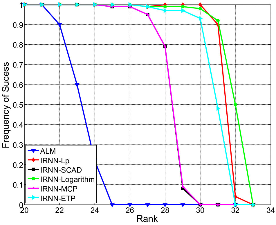
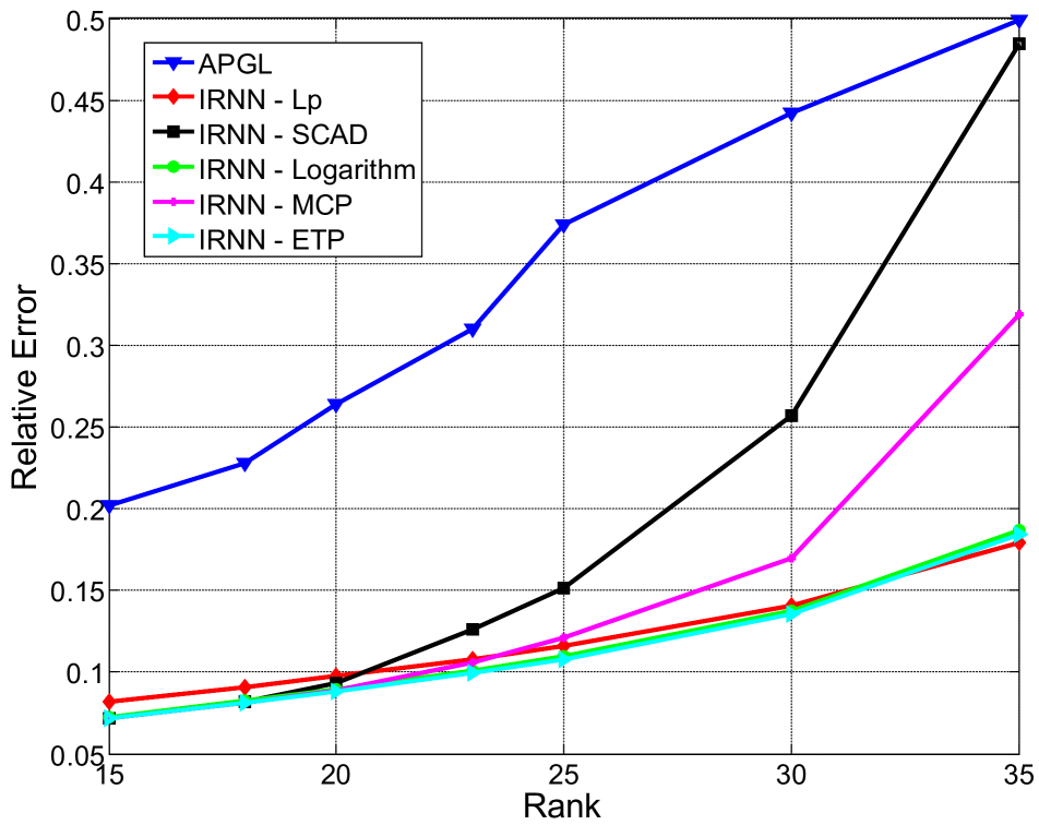
Figure 3: Comparison of matrix recovery on (a) random data without noise, and (b) random data with noise.
Refer to caption
Figure 4: Comparison of image recovery by using different matrix completion algorithms. (a) Original image. (b) Image with Gaussian noise and text. (c)-(g) Recovered images by APGL, LMaFit, TNNR-ADMM, IRNN-Lpsubscript𝐿𝑝L_{p}, and IRNN-SCAD, respectively. Best viewed in ×2absent2\times 2 sized color pdf file.

5 Experiments

In this section, we present several experiments on both synthetic data and real images to validate the effectiveness of the IRNN algorithm. We test our algorithm on the matrix completion problem

min𝐗i=1mgλ(σi(𝐗))+12𝒫Ω(𝐗𝐌)F2,subscript𝐗superscriptsubscript𝑖1𝑚subscript𝑔𝜆subscript𝜎𝑖𝐗12superscriptsubscriptnormsubscript𝒫Ω𝐗𝐌𝐹2\min_{\operatorname*{\mathbf{X}}}\sum_{i=1}^{m}g_{\lambda}(\sigma_{i}(\operatorname*{\mathbf{X}}))+\frac{1}{2}||\mathcal{P}_{\Omega}(\operatorname*{\mathbf{X}}-\operatorname*{\mathbf{M}})||_{F}^{2}, (35)

where ΩΩ\Omega is the set of indices of samples, and 𝒫Ω:m×nm×n:subscript𝒫Ωsuperscript𝑚𝑛superscript𝑚𝑛\mathcal{P}_{\Omega}:\mathbb{R}^{m\times n}\rightarrow\mathbb{R}^{m\times n} is a linear operator that keeps the entries in ΩΩ\Omega unchanged and those outside ΩΩ\Omega zeros. The gradient of squared loss function in (35) is Lipschitz continuous, with a Lipschitz constant L(f)=1𝐿𝑓1L(f)=1. We set μ=1.1𝜇1.1\mu=1.1 in Algorithm 1. For the choice of gλsubscript𝑔𝜆g_{\lambda}, we test all the penalty functions listed in Table 1 except for Capped L1subscript𝐿1L_{1} and Geman, since we find that their recovery performances are sensitive to the choices of γ𝛾\gamma and λ𝜆\lambda in different cases. For the choice of λ𝜆\lambda in IRNN, we use a continuation technique to enhance the low-rank matrix recovery. The initial value of λ𝜆\lambda is set to a larger value λ0subscript𝜆0\lambda_{0}, and dynamically decreased by λ=ηkλ0𝜆superscript𝜂𝑘subscript𝜆0\lambda=\eta^{k}\lambda_{0} with η<1𝜂1\eta<1. It is stopped till reaching a predefined target λtsubscript𝜆𝑡\lambda_{t}. 𝐗𝐗\operatorname*{\mathbf{X}} is initialized as a zero matrix. For the choice of parameters (e.g., p𝑝p and γ𝛾\gamma) in the nonconvex penalty functions, we search it from a candidate set and use the one which obtains good performance in most cases 111Code of IRNN: https://sites.google.com/site/canyilu/..

5.1 Low-Rank Matrix Recovery

We first compare our nonconvex IRNN algorithm with state-of-the-art convex algorithms on synthetic data. We conduct two experiments. One is for the observed matrix 𝐌𝐌\operatorname*{\mathbf{M}} without noise, and the other one is for 𝐌𝐌\operatorname*{\mathbf{M}} with noise.

For the noise free case, we generate the rank r𝑟r matrix 𝐌𝐌\operatorname*{\mathbf{M}} as 𝐌L𝐌Rsubscript𝐌𝐿subscript𝐌𝑅\operatorname*{\mathbf{M}}_{L}\operatorname*{\mathbf{M}}_{R}, where 𝐌L150×rsubscript𝐌𝐿superscript150𝑟\operatorname*{\mathbf{M}}_{L}\in\mathbb{R}^{150\times r}, and 𝐌Rr×150subscript𝐌𝑅superscript𝑟150\operatorname*{\mathbf{M}}_{R}\in\mathbb{R}^{r\times 150} are generated by the Matlab command dn. 50%percent5050\% elements of 𝐌𝐌\operatorname*{\mathbf{M}} are missing uniformly at random. We compare our algorithm with Augmented Lagrange Multiplier (ALM) 222Code: http://perception.csl.illinois.edu/matrix-rank/sample_code.html. [17] which solves the noise free problem

min𝐗𝐗 s.t. 𝒫Ω(𝐗)=𝒫Ω(𝐌).subscript𝐗subscriptnorm𝐗 s.t. subscript𝒫Ω𝐗subscript𝒫Ω𝐌\min_{\operatorname*{\mathbf{X}}}||\operatorname*{\mathbf{X}}||_{*}\ \text{ s.t. }\ \mathcal{P}_{\Omega}(\operatorname*{\mathbf{X}})=\mathcal{P}_{\Omega}(\operatorname*{\mathbf{M}}). (36)

For this task, we set λ0=𝒫Ω(𝐌)subscript𝜆0subscriptnormsubscript𝒫Ω𝐌\lambda_{0}=||\mathcal{P}_{\Omega}(\operatorname*{\mathbf{M}})||_{\infty}, λt=105λ0subscript𝜆𝑡superscript105subscript𝜆0\lambda_{t}=10^{-5}\lambda_{0}, and η=0.7𝜂0.7\eta=0.7 in IRNN, and stop the algorithm when 𝒫Ω(𝐗𝐌)F105subscriptnormsubscript𝒫Ω𝐗𝐌𝐹superscript105||\mathcal{P}_{\Omega}(\operatorname*{\mathbf{X}}-\operatorname*{\mathbf{M}})||_{F}\leq 10^{-5}. For ALM, we use the default parameters in the released codes. We evaluate the recovery performance by the Relative Error defined as 𝐗^𝐌F/𝐌F,subscriptnorm^𝐗𝐌𝐹subscriptnorm𝐌𝐹||\hat{\operatorname*{\mathbf{X}}}-\operatorname*{\mathbf{M}}||_{F}/||\operatorname*{\mathbf{M}}||_{F}, where 𝐗^^𝐗\hat{\operatorname*{\mathbf{X}}} is the recovered solution by a certain algorithm. If the Relative Error is smaller than 103superscript10310^{-3}, 𝐗^^𝐗\hat{\operatorname*{\mathbf{X}}} is regarded as a successful recovery of 𝐌𝐌\operatorname*{\mathbf{M}}. We repeat the experiments 100 times with the underlying rank r𝑟r varying from 20 to 33 for each algorithm. The frequency of success is plotted in Figure 3(a). The legend IRNN-Lpsubscript𝐿𝑝L_{p} in Figure 3(a) denotes the Lpsubscript𝐿𝑝L_{p} penalty function used in problem (1) and solved by our proposed IRNN algorithm. It can be seen that IRNN with all the nonconvex penalty functions achieves much better recovery performance than the convex ALM algorithm. This is because the nonconvex penalty functions approximate the rank function better than the convex nuclear norm.

For the noisy case, the data are generated by 𝒫Ω(𝐌)=𝒫Ω(𝐌L𝐌R)subscript𝒫Ω𝐌subscript𝒫Ωsubscript𝐌𝐿subscript𝐌𝑅\mathcal{P}_{\Omega}(\operatorname*{\mathbf{M}})=\mathcal{P}_{\Omega}(\operatorname*{\mathbf{M}}_{L}\operatorname*{\mathbf{M}}_{R})+0.1×\timesdn. We compare our algorithm with convex Accelerated Proximal Gradient with Line search (APGL) 333Code: http://www.math.nus.edu.sg/~mattohkc/NNLS.html. [20] which solves the noisy problem

min𝐗λ𝐗+12𝒫Ω(𝐗)𝒫Ω(𝐌)F2.subscript𝐗𝜆subscriptnorm𝐗12superscriptsubscriptnormsubscript𝒫Ω𝐗subscript𝒫Ω𝐌𝐹2\min_{\operatorname*{\mathbf{X}}}\lambda||\operatorname*{\mathbf{X}}||_{*}+\frac{1}{2}||\mathcal{P}_{\Omega}(\operatorname*{\mathbf{X}})-\mathcal{P}_{\Omega}(\operatorname*{\mathbf{M}})||_{F}^{2}. (37)

For this task, we set λ0=10𝒫Ω(𝐌)subscript𝜆010subscriptnormsubscript𝒫Ω𝐌\lambda_{0}=10||\mathcal{P}_{\Omega}(\operatorname*{\mathbf{M}})||_{\infty}, and λt=0.1λ0subscript𝜆𝑡0.1subscript𝜆0\lambda_{t}=0.1\lambda_{0} in IRNN. All the chosen algorithms are run 100 times with the underlying rank r𝑟r lying between 15 and 35. The relative errors can be ranging for each test, and the mean errors by different methods are plotted in Figure 3(b). It can be seen that IRNN for the nonconvex penalty outperforms the convex APGL for the noisy case. Note that we cannot conclude from Figure 3 that IRNN with Lpsubscript𝐿𝑝L_{p}, Logarithm and ETP penalty functions always perform better than SCAD and MCP, since the obtained solutions are not globally optimal.

5.2 Application to Image Recovery

In this section, we apply matrix completion for image recovery. As shown in Figure 4, the real image may be corrupted by different types of noises, e.g., Gaussian noise or unrelated text. Usually the real images are not of low-rank, but the top singular values dominate the main information [16]. Thus the corrupted image can be recovered by low-rank approximation. For color images which have three channels, we simply apply matrix completion for each channel independently. The well known Peak Signal-to-Noise Ratio (PSNR) is employed to evaluate the recovery performance. We compare IRNN with some other matrix completion algorithms which have been applied for this task, including APGL, Low-Rank Matrix Fitting (LMaFit) 444Code: http://lmafit.blogs.rice.edu/.. [22] and Truncated Nuclear Norm Regularization (TNNR) [16]. We use the solver based on ADMM to solve a subproblem of TNNR in the released codes (denoted as TNNR-ADMM) 555Code: https://sites.google.com/site/zjuyaohu/.. We try to tune the parameters to be optimal of the chosen algorithms and report the best result.

Refer to caption
Figure 5: Comparison of image recovery on more images. (a) Original images. (b) Images with noises. Recovered images by (c) APGL, and (d) IRNN-Lpsubscript𝐿𝑝L_{p}. Best viewed in ×2absent2\times 2 sized color pdf file.

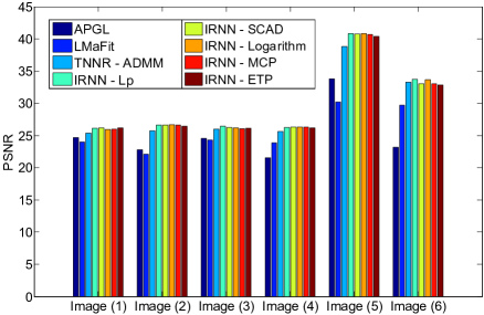
In our test, we consider two types of noises on the real images. The first one replaces 50%percent5050\% of pixels with random values (sample image (1) in Figure 4 (b)). The other one adds some unrelated texts on the image (sample image (2) in Figure 4 (b)). Figure 4 (c)-(g) show the recovered images by different methods. It can be observed that our IRNN method with different penalty functions achieves much better recovery performance than APGL and LMaFit. Only the results by IRNN-Lpsubscript𝐿𝑝L_{p} and IRNN-SCAD are plotted due to the limit of space. We further test on more images and plot the results in Figure 5. Figure 6 shows the PSNR values of different methods on all the test images. It can be seen that IRNN with all the evaluated nonconvex functions achieves higher PSNR values, which verifies that the nonconvex penalty functions are effective in this situation. The nonconvex truncated nuclear norm is close to our methods, but its running time is 3similar-to\sim5 times of that for ours.

6 Conclusions and Future Work

In this work, the nonconvex surrogate functions of L0subscript𝐿0L_{0}-norm are extended on the singular values to approximate the rank function. It is observed that all the existing nonconvex surrogate functions are concave and monotonically increasing on [0,)0[0,\infty). Then a general solver IRNN is proposed to solve problem (1) with such penalties. IRNN is the first algorithm which is able to solve the general nonconvex low-rank minimization problem (1) with convergence guarantee. The nonconvex penalty can be nonsmooth by using the supergradient at the nonsmooth point. In theory, we proved that any limit point is a local minimum. Experiments on both synthetic data and real images demonstrated that IRNN usually outperforms the state-of-the-art convex algorithms. An interesting future work is to solve the nonconvex low-rank minimization problem with affine constraint. A possible way is to combine IRNN with Alternating Direction Method of Multiplier (ADMM).
Refer to caption
Figure 6: Comparison of the PSNR values by different matrix completion algorithms.

Acknowledgements

This research is supported by the Singapore National Research Foundation under its International Research Centre @Singapore Funding Initiative and administered by the IDM Programme Office. Z. Lin is supported by NSF of China (Grant nos. 61272341, 61231002, and 61121002) and MSRA.

References

  • [1] Y. Amit, M. Fink, N. Srebro, and S. Ullman. Uncovering shared structures in multiclass classification. In ICML, 2007.
  • [2] A. Argyriou, T. Evgeniou, and M. Pontil. Convex multi-task feature learning. Machine Learning, 2008.
  • [3] A. Beck and M. Teboulle. A fast iterative shrinkage-thresholding algorithm for linear inverse problems. SIAM Journal on Imaging Sciences, 2009.
  • [4] D. P. Bertsekas. Nonlinear programming. Athena Scientific (Belmont, Mass.), 2nd edition, 1999.
  • [5] K. Border. The supergradient of a concave function. http://www.hss.caltech.edu/~kcb/Notes/Supergrad.pdf, 2001. [Online].
  • [6] E. Candès and T. Tao. The power of convex relaxation: Near-optimal matrix completion. IEEE Transactions on Information Theory, 2010.
  • [7] E. Candès, M. Wakin, and S. Boyd. Enhancing sparsity by reweighted 1subscript1\ell_{1} minimization. Journal of Fourier Analysis and Applications, 2008.
  • [8] K. Chen, H. Dong, and K. Chan. Reduced rank regression via adaptive nuclear norm penalization. Biometrika, 2013.
  • [9] F. Clarke. Nonsmooth analysis and optimization. In Proceedings of the International Congress of Mathematicians, 1983.
  • [10] J. Fan and R. Li. Variable selection via nonconcave penalized likelihood and its oracle properties. Journal of the American Statistical Association, 2001.
  • [11] L. Frank and J. Friedman. A statistical view of some chemometrics regression tools. Technometrics, 1993.
  • [12] J. Friedman. Fast sparse regression and classification. International Journal of Forecasting, 2012.
  • [13] C. Gao, N. Wang, Q. Yu, and Z. Zhang. A feasible nonconvex relaxation approach to feature selection. In AAAI, 2011.
  • [14] G. Gasso, A. Rakotomamonjy, and S. Canu. Recovering sparse signals with a certain family of nonconvex penalties and DC programming. IEEE Transactions on Signal Processing, 2009.
  • [15] D. Geman and C. Yang. Nonlinear image recovery with half-quadratic regularization. TIP, 1995.
  • [16] Y. Hu, D. Zhang, J. Ye, X. Li, and X. He. Fast and accurate matrix completion via truncated nuclear norm regularization. TPAMI, 2013.
  • [17] Z. Lin, M. Chen, L. Wu, and Y. Ma. The augmented lagrange multiplier method for exact recovery of a corrupted low-rank matrices. UIUC Technical Report UILU-ENG-09-2215, Tech. Rep., 2009.
  • [18] G. Liu, Z. Lin, S. Yan, J. Sun, Y. Yu, and Y. Ma. Robust recovery of subspace structures by low-rank representation. TPAMI, 2013.
  • [19] K. Mohan and M. Fazel. Iterative reweighted algorithms for matrix rank minimization. In JMLR, 2012.
  • [20] K. Toh and S. Yun. An accelerated proximal gradient algorithm for nuclear norm regularized linear least squares problems. Pacific Journal of Optimization, 2010.
  • [21] J. Trzasko and A. Manduca. Highly undersampled magnetic resonance image reconstruction via homotopic 0subscript0\ell_{0}-minimization. TMI, 2009.
  • [22] Z. Wen, W. Yin, and Y. Zhang. Solving a low-rank factorization model for matrix completion by a nonlinear successive over-relaxation algorithm. Mathematical Programming Computation, 2012.
  • [23] C. Zhang. Nearly unbiased variable selection under minimax concave penalty. The Annals of Statistics, 2010.
  • [24] T. Zhang. Analysis of multi-stage convex relaxation for sparse regularization. JMLR, 2010.