A semi-parametric Bayesian model of inter- and intra-examiner agreement for periodontal probing depth

Abstract

Periodontal probing depth is a measure of periodontitis severity. We develop a Bayesian hierarchical model linking true pocket depth to both observed and recorded values of periodontal probing depth, while permitting correlation among measures obtained from the same mouth and between duplicate examiners’ measures obtained at the same periodontal site. Periodontal site-specific examiner effects are modeled as arising from a Dirichlet process mixture, facilitating identification of classes of sites that are measured with similar bias. Using simulated data, we demonstrate the model’s ability to recover examiner site-specific bias and variance heterogeneity and to provide cluster-adjusted point and interval agreement estimates. We conclude with an analysis of data from a probing depth calibration training exercise.

and t1Supported in part by NIH Grants K25DE016863, P20RR017696, U24DE016508 and P30CA138313. t2Supported in part by NSF Grant DMS0604666, and by NIH Grants P20RR017696, R01DE16353, R03DE020114, R03CA137805 and U24DE016508.

1 Introduction

Periodontitis is a chronic infectious disease characterized by gingival bleeding and attachment loss, an increase in pocket depth (the distance from the gingival crest to the base of the periodontal pocket), and bone loss. Periodontitis is diagnosed using measures of clinical attachment loss and probing depth, and the present analysis concerns examiner agreement with respect to the latter.

1.1 Data description

The motivating data were obtained from a calibration exercise for dental hygienists in the clinical core of the South Carolina Center of Biomedical Research Excellence for Oral Health at the Medical University of South Carolina. These data are from a pilot calibration study used to obtain preliminary measures of agreement and corresponding uncertainty. Results were used subsequently to design a formal examiner calibration study described elsewhere [Hill et al. (2006)].

Periodontitis is a periodontal site-specific disease, meaning that one site may be severely affected, while a neighboring site on the same tooth remains unaffected. For this reason, pocket depth is measured using a manual probe at six sites on the same tooth: the distobuccal, midbuccal, mesiobuccal, distolingual, midlingual, and mesiolingual. Buccal sites are those nearest the cheek or lips, lingual sites are those nearest the tongue, and distal and mesial sites are those farthest from and closest to the midline of the dental arch, respectively. To facilitate development of the model presented in Section 2, we distinguish between the following quantities: (1) pocket depth, the true biological state; (2) observed probing depth, the manually probed measure of pocket depth observed on a continuum; and (3) recorded probing depth, equal to the greatest integer less than or equal to the observed probing depth. The collection of recorded probing depths comprise the recorded data for the purposes of analysis.

Prior to formal examiner calibration, a pilot calibration exercise was devised to provide initial assessment of examiners’ performance and identify areas in which examiners required additional training. In this study, a standard examiner (S)—an experienced periodontist with extensive training in periodontal research techniques—provided initial training for each of three dental hygienists (A, B and C) in basic methodology for clinical research and correct procedures for performing standardized periodontal examinations. The pilot calibration study was designed so that the standard and all hygienists measured pocket depth at all six periodontal sites of all teeth except third molars and teeth restored with implants. Probing depth was recorded as the largest whole millimeter less than or equal to the value observed on a manual probe, with minimum and maximum allowable probing depth measures of 0 mm and 15 mm, respectively.

A randomization sequence was used to assign examiner pairs to all quadrants—upper right, upper left, lower left and lower right—of calibration subjects. This scheme guaranteed examiners evaluated an equal number of quadrants from the upper and lower arches, and right and left sides. Probing depth measurements were obtained from nine subjects, and both inter- (AS, BS, CS, AB, AC and BC) and intra-examiner (AA, BB, CC and SS) data were collected. Each site was probed by exactly two examiners since pocket depth may increase with additional repeat probings [Osborn et al. (1992)]. Measures of a site by the same examiner contributed to intra-examiner assessment, while those from different examiners were used to evaluate inter-examiner agreement. Thus, a fully dentate calibration subject contributes 336 site-level measurements (28 teeth${}\times{}$6 sites per tooth${}\times{}$2 examiner measurements per site) from which we obtain examiner-pair calibration indices reflecting agreement at the level of the periodontal site.

1.2 Measuring agreement

In a separate analysis of these data, Hill et al. (2006) demonstrate the need to account for within-subject correlation among site-level binary indices of agreement. They report cluster-adjusted point and interval estimates of percent exact agreement and agreement within 1 mm for probing depth, with confidence intervals constructed as described by Cochran [Cochran (1977), pages 240–270]. For this pilot calibration data, the asymptotics of the variance estimator for the cluster-adjusted sample proportion are compromised due to two dominant data characteristics: (1) the number of clusters (subjects) for a given examiner pair is small (range${}={}$1 to 5); and (2) for a given examiner pair, the cluster sizes are large relative to the number of clusters (average cluster size${}={}$35 periodontal sites). Of the 20 cluster-adjusted 95% confidence intervals for percent agreement (exact or within 1 mm) of probing depth reported by Hill et al. (2006), one is truncated at 0%, nine are truncated at 100%, two are nonestimable because the point estimate is constructed from a single cluster, and one is nonestimable because the within-cluster estimates of agreement are equal. We note that estimating the uncertainty associated with any agreement measure (e.g., weighted kappa or intra-cluster correlation) is complicated by these data limitations.

Other authors have addressed the issue of agreement estimation for correlated observations. Williamson and Manatunga (1997) use a latent variable model to assess examiner agreement in classifying cervical ectopy where the examiners use two different cervical assessment methods. Their model includes random effects to capture both the correlation among ratings from the same subject using different assessment methods, as well as the correlation between ratings obtained from the same examiner using different assessment methods. In another paper, Williamson, Lipsitz and Manatunga (2000) analyze this same data using a pair of generalized estimating equations (GEEs), the first modeling the marginal distribution of the ratings and the second modeling the binary indicator of agreement between two subject-level ratings. Oden (1991) tackles the problem of agreement estimation for correlated binocular ratings. He derives an expression for the approximate variance of a pooled-$\kappa$ estimate for paired left- and right-eye ratings under the assumption that the true left- and right-eye $\kappa$ values are the same.

For our data, we use a Bayesian hierarchical modeling approach and specify three separate but conditionally related models for: (1) pocket depth, with subject-specific random effects capturing the marginal correlation among pocket depths within the same mouth; (2) observed probing depth conditional on pocket depth, with marginal correlation between duplicate observations from the same periodontal site, and a Dirichlet process prior (DPP) on the examiner-bias parameters to accommodate possible latent class structure in examiner effects; and (3) recorded probing depth conditional on observed probing depth, from which the data likelihood is constructed. We simulate data from the posterior predictive distribution to estimate indices of agreement and to obtain corresponding interval estimates corrected for the correlation in these data.

The motivation for our approach is twofold. First, a model-based approach utilizing all the data facilitates borrowing of strength across examiner pairs and helps mitigate problems associated with small numbers of large clusters (here, nine clusters with maximum size of 336). Second, by placing the DPP on model parameters, factors associated with examiner bias need not be specified a priori. Rather, our model learns characteristics associated with bias, and allows these to vary by site, subject and examiner. Investigating such effects in more traditional modeling settings would require specifying in advance all potential main and interaction effects of interest. We describe our model in Section 2 and present results from a simulation study in Section 3. We apply our method to the periodontal probing depth calibration study data and summarize our results in Section 4. We conclude in Section 5 with a discussion of the merits of our approach and identify areas for further research.

2 Model specification

We consider recorded probing depths to be measurements that result from error-prone and biased observations made of unobservable true pocket depth. We therefore construct our hierarchical model by sequentially modeling these phenomena, from truth to data.

2.1 Pocket depth

Among U.S. adults, probing depth follows a positively skewed distribution with the majority of values falling in the 1 mm to 3 mm range; depths greater than 6 mm occur infrequently [Albandar, Brunelle and Kingman (1999)]. Based on this observation and assuming all pockets have positive depth, we model pocket depth using lognormal distributions as described below.

For each of $n$ subjects, $m_{i}$ periodontal sites are examined, where $i=1,\ldots,n$ and $m_{i}$ is the total number of sites examined across all teeth for subject $i$. Let $\theta_{ij}$ be the pocket depth for the $j$th site of the $i$th subject, $j=1,\ldots,m_{i}$. We model the marginal correlation among pocket depths from the same subject using random effects. Specifically, we write

$$\log(\theta_{ij}) = \mu+b_{i}+\varepsilon_{ij},$$ (1)

where $b_{i}|\sigma^{2}_{b}\sim\mathrm{N}(0,\sigma^{2}_{b})$, $\varepsilon_{ij}|\sigma^{2}_{\varepsilon}\sim\mathrm{N}(0,\sigma^{2}_{\varepsilon})$, and $b_{i}$ and $\varepsilon_{ij}$ are assumed independent. This model yields an exchangeable correlation structure in which all sites in the same mouth are equally correlated, a simplifying assumption that has been used previously in the analysis of periodontal data [DeRouen, Mancl and Hujoel (1991)].

2.2 Observed probing depth

Like pocket depth, we assume observed probing depth is positive and follows a lognormal distribution. Let $k=1,2$ index the duplicate observed probing depth measures, $T_{ijk}$, for the $j$th periodontal site of subject $i$. Because $T_{ijk}$ is the probing depth observed by any one of the four examiners, we introduce indicator variables to denote the examiner associated with observation $T_{ijk}$. Hygienists’ performance relative to the standard is of primary importance, and we therefore select the standard as the reference level for the examiner indicator variables. Accordingly, let $X_{E,ijk}$ equal 1 when $T_{ijk}$ is measured by examiner $E={}$A, B or C, and 0 otherwise. Then $\mathbf{X}_{ijk}=(X_{A,ijk},X_{B,ijk},X_{C,ijk})^{\prime}$ consists of all zeros if the examiner is the standard, and is a vector of zeros and a single one otherwise. Let $\beta_{E,ij}$ be the effect, relative to the standard examiner, of examiner $E$ on observed probing depth, so that $\bolds{\beta}_{ij}=(\beta_{A,ij},\beta_{B,ij},\beta_{C,ij})^{\prime}$ is the parameter vector associated with $\mathbf{X}_{ijk}$.

Let $\mathbf{T}_{ij}=(T_{ij1},T_{ij2})^{\prime}$ and model $T_{ijk}$ as

$$\log(T_{ijk}) = \log(\theta_{ij})+\mathbf{X}_{ijk}^{\prime}\bolds{\beta}_{ij}+\gamma_{ijk}.$$ (2)

To accommodate variance heterogeneity across examiners, we model the error terms $\gamma_{ijk}|\mathbf{X}_{ijk},\bolds{\sigma}^{2}\sim\mathrm{N}(0,\tilde{\mathbf{X}}_{ijk}^{\prime}\bolds{\sigma}^{2})$, where $\tilde{\mathbf{X}}_{ijk}=(\mathbf{X}_{ijk}^{\prime},\prod_{E}(1-X_{E,ijk}))^{\prime}$ and $\bolds{\sigma}^{2}=(\sigma_{A}^{2},\sigma_{B}^{2},\sigma_{C}^{2},\sigma_{S}^{2})^{\prime}$. Thus, the $\gamma_{ijk}$ are independent mean zero Gaussian random variables with variance one of $\sigma^{2}_{A}$, $\sigma^{2}_{B}$, $\sigma^{2}_{C}$ or $\sigma^{2}_{S}$ according to the examiner associated with observation $T_{ijk}$. We further assume that $\gamma_{ijk}$ and $b_{i}$, and $\gamma_{ijk}$ and $\varepsilon_{ij}$ are independent. Finally, since $\theta_{ij}$ is a random quantity, duplicate observations ($T_{ij1}$ and $T_{ij2}$) are marginally correlated.

Throughout, we assume the standard examiner exhibits no bias. However, if unbiased measuring behavior for the standard cannot be assumed, then equation (1) represents “truth” as seen by the standard. Our reference model, Model 0, has common examiner variances and no examiner biases. Specifically, $\sigma^{2}_{A}=\sigma^{2}_{B}=\sigma^{2}_{C}=\sigma^{2}_{S}=\sigma^{2}$ and $\bolds{\beta}_{ij}\equiv\mathbf{0}$. We consider three alternative models for observed probing depth described as follows.

2.2.1 Unequal variances and no biases

Model 1 assumes $\bolds{\beta}_{ij}\equiv\mathbf{0}$, but imposes no constraints among the examiner variances. Here examiners may differ in the variability of their probing depth measures, but all are unbiased.

2.2.2 Unequal variances and constant bias

Model 2 relaxes Model 1 by permitting a common examiner effect so that $\beta_{E,ij}=\beta_{E}$ for all $i$ and $j$. Thus, study examiners A, B and C are equally biased for all periodontal sites, but need not have the same bias.

2.2.3 Unequal variances and site-level biases

Model 3 further relaxes assumptions by placing a nonparametric Dirichlet process prior (DPP) on $\beta_{E,ij}$ that supports different effects for examiners A, B and C associated with site-level characteristics. Our motivation is to incorporate flexibility in the examiner bias parameters to facilitate discovery of any latent class structure among the sites. Here classes define collections of sites with common measurement bias, the identification of which may be useful in designing follow-up training for examiners or future calibration exercises. Our approach is similar to that used by Congdon (2007) in which he placed DPPs on regression coefficients in a bivariate analysis of male and female suicides in England to capture spatial variability in the regression parameters.

Escobar and West [Escobar and West (1995, 1998)] describe mixture modeling via DPPs. Congdon (2001), pages 260–273, summarizes their work (and others) and provides examples of DPP mixture modeling using WinBUGS [Lunn et al. (2000)]. To briefly summarize, let $y_{i}$, $i=1,\ldots,n$, be drawn from the distribution $f(y_{i}|\phi_{i})$, where the parameter $\phi_{i}$ is unknown. The DPP treats the underlying distribution of $\phi_{i}$ as unknown but centered around a base distribution, $G_{0}$, from which candidate values for $\phi_{i}$ are drawn according to a concentration parameter, $\alpha$. The $\phi_{i}$ cluster based on similarities among the $y_{i}$, so that assignment of a given candidate value from $G_{0}$ to multiple $\phi_{i}$ may be expected. In practice, $M\leq n$ candidate values, denoted $\phi_{m}^{\ast}$ with $m=1,\ldots,M$, are drawn from $G_{0}$ and $M^{\ast}\leq M$ of these are allocated to one or more of the $\phi_{i}$. The density of $\phi_{i}$ more closely resembles $G_{0}$ for large values of $\alpha$, while small values of $\alpha$ result in a density similar to a finite mixture model. A practical approach to implementation of the DPP using a ‘stick-breaking prior’ is described by Ishwaran and James (2001) and is based on a finite version of the constructive definition introduced by Sethuraman (1994). Our implementation uses this finite approximation.

In our probing depth application, we accommodate different latent class structures across examiners A, B and C, and assign the DPP to the model regression parameters, $\beta_{E,ij}$, as $\beta_{E,ij}|\Gamma_{E}\sim\Gamma_{E}$ with $\Gamma_{E}\sim DP(\alpha_{E}G_{E,0})$. We specify $G_{E,0}$ to be a normal distribution with examiner-specific mean and variance, and $\alpha_{E}$ is a precision parameter. Sites $(i,j)$ and $(i^{\prime},j^{\prime})$ are identified as belonging to the same cluster for examiner $E$ when $\beta_{E,ij}=\beta_{E,i^{\prime}j^{\prime}}$. Congdon (2001) notes the number of classes cannot exceed the number of distinct data values. In our application, recorded probing depth takes integer values ranging from 0 mm to 8 mm, with the difference in duplicate measures ranging from $-$4 mm to 4 mm. These values lead to at most 9 distinct intervals for the observed probing depth and, although $T_{ijk}$ may vary within these intervals, such variation within 1 mm adds little to understanding examiner performance. Since we place separate DPPs on the distribution of $\beta_{E,ij}$ for examiners A, B and C, we use an examiner subscript for the number of candidate values, $M_{E}$, drawn from the baseline distribution, $G_{E,0}$. We used $M_{E}=6$ for all examiners to facilitate sufficient model flexibility to discover latent class structure. We specified a range of potential values for the concentration parameters with $\alpha_{E}=0.5,1,2,3,4,5,6,7,8,9,10$ and $20$ and conducted a sensitivity analysis (summarized in Section 3.1) to facilitate selection. Based on comparisons of posterior class inference across the range of $\alpha_{E}$ values, we selected $\alpha_{E}=8$ for all $E$.

2.3 Recorded probing depth

The translation from observed to recorded probing depth is based on both examination protocol and physical characteristics of the manual probe. The probe is scored at sequential millimeter markings so that observed probing depths fall at or between markings. In our study, probing depths were recorded as the greatest integer less than or equal to the probing depth observed on the manual probe. Although our protocol accommodated recorded probing depths up to 15 mm, the largest recorded value was 8 mm.

Let $U_{ijk}$ be the recorded probing depth for the $k$th replicate of the $j$th site for the $i$th subject. Then

$$U_{ijk} = \cases{\lfloor T_{ijk}\rfloor,&\quad if $0\leq T_{ijk}<15$,\vspace*{3pt}\cr 15,&\quad otherwise,}$$ (3)

where $\lfloor a\rfloor$ is the greatest integer less than or equal to $a$. It follows that

$$\pi_{u,ijk} = \operatorname{Pr}\bigl{(}U_{ijk}=u|\log(\theta_{ij}),\bolds{\beta}_{ij},\mathbf{X}_{ijk},\bolds{\sigma}^{2}\bigr{)}$$

$$= \cases{\zeta_{u+1},&\quad if $u=0$,\cr\zeta_{u+1}-\zeta_{u},&\quad if $u=1,\ldots,14$,\cr 1-\zeta_{u},&\quad if $u=15$,}$$

where $\zeta_{u}=\Phi[\{\log(u)-\log(\theta_{ij})-\mathbf{X}_{ijk}^{\prime}\bolds{\beta}_{ij}\}/\tilde{\mathbf{X}}_{ijk}^{\prime}\bolds{\sigma}^{2}]$ and $\Phi(\cdot)$ is the standard normal distribution function. Let $\mathbf{V}_{ijk}=(V_{0,ijk},V_{1,ijk},\ldots,V_{15,ijk})^{\prime}$ be a vector of length 16 consisting of 15 zeros and a single one such that $V_{u,ijk}=1$ when $U_{ijk}=u$. Then $\mathbf{V}_{ijk}|\log(\theta_{ij}),\bolds{\beta}_{ij},\mathbf{X}_{ijk},\bolds{\sigma}^{2}\sim\operatorname{Multinomial}(1;\bolds{\pi}_{ijk})$, where $\bolds{\pi}_{ijk}=(\pi_{0,ijk},\pi_{1,ijk},\ldots,\pi_{15,ijk})^{\prime}$ and the (conditional) likelihood, $L$, is given by

$$L\propto\prod_{i=1}^{n}\prod_{j=1}^{m_{i}}\prod_{k=1}^{2}\prod_{u=0}^{15}\pi_{u,ijk}^{V_{u,ijk}}.$$ (4)

2.4 Estimation and inference

2.4.1 Prior specifications

For all analyses, we placed diffuse proper priors on the pocket depth model parameters, with $\mu\sim\mathrm{N}(0,1000)$, $\sigma_{b}\sim\operatorname{Uniform}(0,10)$ and $\sigma_{\varepsilon}\sim\operatorname{Uniform}(0,10)$. Likewise, we placed $\operatorname{Uniform}(0,10)$ priors on all standard deviation parameters of the observed probing depth model, $\sigma_{A}$, $\sigma_{B}$, $\sigma_{C}$ and $\sigma_{S}$. For the DPP on the examiner effects, we used the stick-breaking prior of Ishwaran and James (2001) with $G_{E,0}=\mathrm{N}(0,1000)$, $M_{E}=6$ and $\alpha_{E}=8$ for all examiners.

We fit our model using WinBUGS [Lunn et al. (2000)]. We ran three chains and assessed convergence graphically using trace plots and modified Gelman–Rubin statistics [Brooks and Gelman (1998)]. We used the batch-means method of Jones and colleagues [Jones et al. (2006)] to assess the precision with which posterior quantiles of agreement indices (the endpoints of primary interest in our analysis) were estimated. We used a burn-in of 50,500 iterations and conducted inference based on a chain of length 10,000 from the posterior distributions of model parameters. Additionally, we constructed point and interval estimates of agreement (weighted kappa, percent exact agreement and percent agreement within 1 mm) based on 10,000 samples from the posterior predictive distribution of recorded probing depths. We used an Intel Core 2 Quad CPU Windows machine for model fit with a total run time (including monitoring of all nodes) of 1468 minutes (approximately 24 hours) for our data.

2.4.2 Posterior clustering inference

The clustering induced by the DPP on the $\beta_{E,ij}$’s is used to identify examiner-specific classes of biased ratings. (Henceforth the terms ‘cluster’ and ‘class’ are used synonymously.) We used the least-squares clustering approach of Dahl (2006) to identify the most likely clustering among those sampled from its posterior distribution. Specifically, let $\mathbf{c}_{E,1},\ldots,\mathbf{c}_{E,D}$ be $D$ draws from the posterior clustering distribution of the $\beta_{E,ij}$’s. For each clustering $\mathbf{c}_{E}$ in $\mathbf{c}_{E,1},\ldots,\mathbf{c}_{E,D}$, let $\delta(\mathbf{c}_{E})$ be an $\mathcal{L}\times\mathcal{L}$ ($\mathcal{L}=\sum_{i=1}^{n}m_{i}$) association matrix with element $\delta(\mathbf{c}_{E})_{\ell\ell^{\prime}}=1$ indicating the examiner effects associated with sites $\ell$ and $\ell^{\prime}$ jointly classified, and 0 otherwise. Element-wise averaging of the collection of association matrices yields the pairwise probability clustering matrix, $\Delta_{E}$. Examiner E’s least-squares cluster, $\mathbf{c}^{\mathrm{LS}}_{E}$, is the observed clustering from the Markov chain for which the squared deviation of its association matrix, $\delta(\mathbf{c}^{\mathrm{LS}}_{E})$, from the pairwise probability clustering matrix, $\Delta_{E}$, is a minimum. Specifically,

$$\mathbf{c}^{\mathrm{LS}}_{E} = \mathop{\arg\min}_{\mathbf{c}_{E}\in\{\mathbf{c}_{E,1},\ldots,\mathbf{c}_{E,D}\}}\ \sum_{\ell=1}^{\mathcal{L}}\sum_{\ell^{\prime}=1}^{\mathcal{L}}\bigl{(}\delta(\mathbf{c}_{E})_{\ell\ell^{\prime}}-\Delta_{E,\ell\ell^{\prime}}\bigr{)}^{2}.$$

The posterior clustering via Dahl’s algorithm was performed on a 9-node cluster with 72 CPUs using code written by the authors in R (version 2.8.1), and took an average of 615 minutes (approximately 10 hours) of user time to conduct inference for a single examiner.

2.4.3 Understanding class membership

For each examiner, we examined the posterior density estimates of the $\beta_{E,ij}$’s for sites in a common class to shed light on the magnitude and direction of bias if present. Additionally, following Fleiss et al. (1991), we examined the association of tooth position (anterior versus posterior, and maxillary versus mandibular) and site location (proximal versus mid-tooth, and lingual versus buccal) with site class membership. We compared the proportion of sites with specified tooth and location characteristics between classes using generalized estimating equations (to accommodate within-mouth clustering).

3 Model evaluation

3.1 Data simulation model

Due to the extensive run time to both fit the model and conduct posterior clustering inference for three examiners, we conducted a simulation using a single data realization. While generalizability of findings are necessarily limited, we explored the model’s ability to recover-known parameter values and measures of agreement based on draws from the joint posterior and posterior predictive distributions, respectively. We constructed the simulated data to reflect the calibration study’s experimental design and resulting structure of the data. Accordingly, we simulated data composed of pocket depths for each of nine subjects using equation (1) with $\mu=1$, $\sigma_{b}=0.2$ and $\sigma_{\varepsilon}=0.3$. For simplicity, we assumed each subject was fully dentate, resulting in a total of 1512 simulated pocket depths. We modeled duplicates of observed probing depth conditional on pocket depth by specifying examiner biases dependent on site-specific characteristics as follows:

$$\qquad\log(T_{ijk}) = \log(\theta_{ij})+\beta_{B,ij}\cdot I(\theta_{ij}\geq 4\mbox{ mm})\cdot I(E=B)$$

$${}+\bigl{[}\beta_{C_{1},ij}+\beta_{C_{2},ij}\cdot I(\mbox{site }j\mbox{ is DLMM})\bigr{]}\cdot I(E=C)+\gamma_{ijk},$$

where $I(\cdot)$ is a binary indicator for the stated condition (DLMM${}={}$distolingual mandibular molar), $\beta_{B,ij}=-0.5$, $\beta_{C_{1},ij}=0.25$, and $\beta_{C_{2},ij}=-1$. The examiner-specific effects expressed in equation (3.1) indicate that, relative to the standard: (1) examiner A does not exhibit biased measuring behavior; (2) examiner B’s measurements on pockets of 4 mm or more are too shallow by 0.5 mm on average; and (3) overall, examiner C’s measures are too deep by 0.25 mm with the exception of distolingual mandibular molar sites, for which measures are negatively biased by 0.75 mm. We further simulated observed probing depths with $\sigma_{A}=0.1,\sigma_{B}=0.25,\sigma_{C}=0.15$ and $\sigma_{S}=0.07$. We then constructed recorded probing depths as described by equation (3). A total of 3024 (1512 pocket depths${}\times{}$2 recorded probing depths per site) simulated recorded probing depths comprised the final simulation data set. Of the sites examined by B, 82 had true depths of 4 mm or more. Of those examined by C, 28 were from distolingual mandibular molars.

We conducted a sensitivity analysis to tune our selection of the concentration parameter, $\alpha_{E}$. Specifically, we considered values of $\alpha_{E}$ equal to 0.5, 1, 2, 3, 4, 5, 6, 7, 8, 9, 10 and 20, and conducted posterior clustering inference using the method of least-squares clustering introduced by Dahl (2006) and described in Section 2.4.2. For each value of $\alpha_{E}$ we assessed both the number of clusters identified as well as the strength of association between class membership and factors known to be associated with biased measurement (e.g., deep pockets for examiner B and distolingual mandibular molars for examiner C). We selected $\alpha_{E}=8$ based on the resulting model’s ability to recover the correct number of clusters for each examiner (1 for A and 2 for B and C), maximum sensitivity and specificity of the recovered cluster assignments, and statistical significance of association of class membership with characteristics inducing bias.

Using the simulated recorded measures as data, we fit Model 3 as described by equations (1), (2) and (4), with examiner-specific variances and site-level examiner biases modeled as described in Section 2.2.3.

3.2 Simulation results

We summarize first our assessment of inter- and intra-examiner agreement, as this was the primary objective of our analysis. For each agreement index, we report three values: the true value, derived from true joint and marginal probabilities of recorded probing depths based on the model described in Section 3.1; the observed value, calculated from the estimated joint and marginal probabilities of recorded probing depths based on the single simulated set of recorded probing depths derived from the model described in Section 3.1; and the median and 95% predictive interval obtained from 10,000 estimates of each agreement measure based on the same number of data realizations derived from the posterior predictive distribution using the analysis model described in Section 3.1. We begin with a detailed description of our approach to agreement evaluation in Sections 3.2.1 through 3.2.4.

3.2.1 True agreement measures

We derived true agreement values based on theoretical joint and marginal probabilities of recorded probing depths. Consider the following example based on examiners B and S. Let $T_{B}$ and $T_{S}$ be observed probing depth duplicates measured by examiners B and S, respectively, for a given periodontal site with corresponding pocket depth $\theta$. From equation (2), the joint distribution of $T_{B}$ and $T_{S}$ is given by

$$\bigl{(}\log(T_{B}),\log(T_{S})\bigr{)}^{\prime} \sim \mathrm{N}(\bolds{\mu},\bolds{\Sigma}),$$ (6)

where $\bolds{\mu}=(\mu-0.5,\mu)^{\prime}$ if $\theta\geq 4$ mm, $\bolds{\mu}=(\mu,\mu)^{\prime}$ if $\theta<4$ mm, $\Sigma_{11}=\sigma^{2}_{b}+\sigma^{2}_{\varepsilon}+\sigma^{2}_{B}$, $\Sigma_{22}=\sigma^{2}_{b}+\sigma^{2}_{\varepsilon}+\sigma^{2}_{S}$, and $\Sigma_{12}=\Sigma_{21}=\sigma^{2}_{b}+\sigma^{2}_{\varepsilon}$. Defining $\eta=\operatorname{Pr}(\theta\geq 4\mbox{~{}mm})=1-\Phi\{(\log 4-\mu)/\sqrt{\Sigma_{12}}\}$, the respective marginal distributions of observed probing depths are

$$\log(T_{B}) \sim \mathrm{N}(\mu-0.5,\Sigma_{11})\eta+\mathrm{N}(\mu,\Sigma_{11})(1-\eta)$$ (7)

and

$$\log(T_{S}) \sim \mathrm{N}(\mu,\Sigma_{22}).$$ (8)

Based on the compound symmetry induced by equation (1), distributions of observed probing depths for other sites within the same mouth are equivalent. Joint and marginal probabilities of recorded probing depths for other examiner pairs are similarly derived.

Weighted kappa, $\kappa_{w}$, is a chance-corrected agreement measure that weights disagreements based on the measures’ relative distance [Cohen (1968); Fleiss (2001), pages 223–225]. Continuing with our example, let $U_{B}$ and $U_{S}$ be recorded probing depths corresponding to observed values $T_{B}$ and $T_{S}$. Define $p_{u_{1},u_{2}}=\operatorname{Pr}(U_{B}=u_{1},U_{S}=u_{2})$, $p_{u_{1}}=\operatorname{Pr}(U_{B}=u_{1})$, and $p_{u_{2}}=\operatorname{Pr}(U_{S}=u_{2})$. Then $\kappa_{w}$ is defined as $\kappa_{w}=(p_{o(w)}-p_{e(w)})/(1-p_{e(w)})$, where $p_{o(w)}=\sum_{u_{1}=0}^{15}\sum_{u_{2}=0}^{15}w_{u_{1},u_{2}}p_{u_{1},u_{2}}$, and $p_{e(w)}=\sum_{u_{1}=0}^{15}\sum_{u_{2}=0}^{15}w_{u_{1},u_{2}}p_{u_{1}}p_{u_{2}}$. We use the common weighting scheme $w_{u_{1},u_{2}}=1-\{(u_{1}-u_{2})^{2}/(N-1)^{2}\}$, where $N$ is the total number of categories (16 in this case).

We also constructed measures of percent exact agreement, $P_{\mathrm{exact}}$, and percent agreement within 1 mm, $P_{\pm 1}$, where $P_{\mathrm{exact}}=\sum_{u=0}^{15}\operatorname{Pr}(U_{B}=U_{S}=u)$ and

$$P_{\pm 1} = P_{\mathrm{exact}}+\sum_{u=1}^{15}\bigl{\{}\operatorname{Pr}(U_{B}=u,U_{S}=u-1)+\mbox{Pr}(U_{B}=u-1,U_{S}=u)\bigr{\}}.$$

We constructed the true value of $\kappa_{w}$ for each examiner pair using the true values of $p_{u_{1}}$, $p_{u_{2}}$ and $p_{u_{1},u_{2}}$ obtained from the joint and marginal distributions shown in (6)–(8) (or analagous distributions for other examiners), and the relationship between observed and recorded probing depths described by equation (3). In a similar manner, we constructed true values of $P_{\mathrm{exact}}$ and $P_{\pm 1}$. The resulting agreement values for each examiner pair are reported in the column labeled “Truth” in Table 1.

Table 1: Simulation agreement results. A, B, C and S are the three examiners and standard. PD${}={}$pocket depth. AS, BS and CS results are based on 210 site-level measures from 5 subjects. Results for all other pairings are based on 126 measures from 3 subjects. Observed results are point estimates obtained from the simulated data set, and results obtained from the posterior predictive distribution are medians and 95% predictive intervals

	Truth			Observed			Post pred
		%			%			%
Pair	$\bolds{\kappa_{w}}$	agree	% $\bolds{\pm 1}$	$\bolds{\kappa_{w}}$	agree	% $\bolds{\pm 1}$	$\bolds{\kappa_{w}}$	agree	% $\bolds{\pm 1}$
AS	0.890	72.2	$99.5$	0.902	66.7	$100.0$	0.846	66.2	99.1
							(0.765, 0.927)	(55.7, 76.7)	(95.7, 100.0)
BS	0.693	44.9	$89.3$	0.454	51.0	$83.3$	0.669	45.2	90.0
							(0.550, 0.819)	(34.8, 57.1)	(80.5, 96.2)
CS	0.664	31.4	$81.3$	0.591	31.0	$79.0$	0.613	31.4	79.1
							(0.498, 0.770)	(22.4, 43.3)	(66.7, 90.0)
AB	0.683	44.0	$88.5$	0.429	48.4	$88.9$	0.633	43.7	88.9
							(0.474, 0.801)	(31.8, 57.1)	(77.0, 96.8)
AC	0.659	31.7	$80.8$	0.709	28.6	$77.8$	0.586	31.0	78.6
							(0.449, 0.762)	(19.8, 45.2)	(62.7, 91.3)
BC	0.547	26.5	$70.5$	0.454	34.1	$81.7$	0.497	26.2	70.6
							(0.332, 0.694)	(16.7, 38.9)	(54.8, 85.7)
AA	0.872	68.1	$99.0$	0.825	64.3	$98.4$	0.835	65.1	98.4
							(0.730, 0.923)	(50.8, 77.8)	(93.7, 100.0)
BB	0.559	35.8	$79.8$	0.344	33.3	$83.3$	0.619	42.1	85.7
							(0.441, 0.789)	(29.4, 55.6)	(73.0, 95.2)
CC	0.719	43.1	$84.5$	0.845	54.0	$88.9$	0.819	48.4	91.3
							(0.712, 0.907)	(35.7, 63.5)	(81.0, 98.4)
SS	0.911	77.2	$99.8$	0.884	70.6	$100.0$	0.872	72.2	100.0
							(0.776, 0.947)	(59.5, 84.1)	(96.8, 100.0)
A/PD	0.910	77.0	$99.8$				0.873	71.8	99.3
							(0.815, 0.939)	(63.6, 79.6)	(97.6, 100.0)
B/PD	0.703	45.9	$90.1$				0.696	46.8	91.2
							(0.611, 0.830)	(38.6, 56.8)	(84.0, 95.9)
C/PD	0.669	30.9	$81.9$				0.629	31.3	80.1
							(0.545, 0.779)	(23.5, 42.0)	(69.6, 89.5)
S/PD	0.936	83.8	$100.0$				0.917	80.3	100.0
							(0.875, 0.963)	(72.9, 86.5)	(99.5, 100.0)

3.2.2 Observed agreement

Additionally, for each examiner pair we constructed empirical estimates of $\kappa_{w}$, $P_{\mathrm{exact}}$ and $P_{\pm 1}$ based on estimated joint and marginal probabilities of recorded probing depths from the simulated data set described in Section 3.1. These values are reported in the column labeled “Observed” in Table 1, and are obtained by using sample proportions to estimate the probabilities required to construct the agreement measures.

3.2.3 Posterior predictive agreement estimates

We also obtained point and interval estimates of agreement for each examiner pair from 10,000 data realizations obtained from the posterior predictive distribution based on the Bayesian analysis model described in Section 3.1. Specifically, for each data set simulated from the posterior predictive distribution, we estimated joint and marginal probabilities of recorded probing depths based on sample proportions, and subsequently constructed estimates of $\kappa_{w}$, $P_{\mathrm{exact}}$ and $P_{\pm 1}$ for each examiner pair. These values are reported in the column labeled “Post pred” in Table 1.

3.2.4 Examiner agreement with pocket depth

We define examiner agreement with true pocket depth as the value of the agreement measure achieved when the collection of recorded probing depths associated with a given examiner, $\{U_{ijk}\}$, are compared to the corresponding values of true pocket depths censored according to the rule described in equation (3). We derived both true measures of agreement based on theoretical joint and marginal probabilities as well as point and interval estimates of agreement resulting from the 10,000 data realizations from the posterior predictive distribution and summarize these results in Table 1. Because truth is not observable, we omit a measure of “Observed” agreement with true pocket depth.

3.2.5 Simulation agreement summary

Although results based on a single simulated data set preclude generalizability, the observations summarized herein are meant to provide a “first look” at model performance. Agreement measures for the simulated data are summarized in Table 1. We observe that estimates based on the posterior predictive distribution recover agreement indices’ true values with all 95% predictive intervals containing the truth, although we can make no claims pertaining to coverage. Still, there are advantages in using repeated draws from the posterior predictive distribution to construct these indices. The ability to obtain interval estimates correctly accounting for the correlation of pocket depths in the same mouth and between duplicate readings is a strength. Furthermore, only the model-based approach provides an estimate of agreement between each examiner and true pocket depth. Finally, since the posterior predictive draws are sampled from a distribution derived from a model utilizing the complete data, the pooling of information yields improved power to make inferential statements about individual examiners.

3.2.6 Model parameters

Table 2 shows posterior estimates of all model parameters (except the $\beta_{E,ij}$’s). Supplementary Figure 1 [Hill and Slate (2014)] shows posterior density estimates of the $\beta_{E,ij}$’s for examiners A, B and C. The posteriors for A effects are strongly unimodal and centered at zero, indicating no bias. In contrast, posterior densities for examiner B effects indicate two modes, one at 0 and another at $-$0.5. Similarly, posterior densities for examiner C effects identify two modes, one at 0.25 and the second at $-$0.75. The locations of these modes are consistent with the data simulation model described by equation (3.1).

=230pt Parameter Truth Posterior estimate $\mu$ $1$ $1.03\ (0.80,1.18)$ $\sigma_{b}$ $0.2$ $0.19\ (0.11,0.40)$ $\sigma_{\varepsilon}$ $0.3$ $0.29\ (0.28,0.30)$ $\sigma_{A}$ $0.1$ $0.11\ (0.09,0.13)$ $\sigma_{B}$ $0.25$ $0.24\ (0.22,0.28)$ $\sigma_{C}$ $0.15$ $0.15\ (0.12,0.17)$ $\sigma_{S}$ $0.07$ $0.08\ (0.07,0.10)$ A classes $1$ 1tt10 (0.07, 0.10) B classes $2$ $2$ C classes $2$ $2$ tt1Two additional classes included a single site each.

Table 2: Simulation model posterior parameter estimates (median and 95% predictive interval). For each examiner, we report the true and estimated number of classes as determined by the method of least-squares clustering

A number of the $\beta_{E,ij}$’s posterior density estimates are bimodal, suggesting, perhaps, that examiner effects sometimes suffer from nonidentifiability. This is most pronounced for examiner pairings without the standard, situations in which there is less information to “anchor” true pocket depth ($\theta_{ij}$). Still, the modes and their relative heights inform on rating behavior: examiner A’s measures are unbiased; examiner B’s measures are most often unbiased but sometimes negatively biased; and examiner C’s measures are most often positively biased but sometimes negatively biased. This information together with the least-squares cluster assignment of the examiner effects provides a picture of both the magnitude of bias as well as those factors influencing bias.

In our simulation, the least-squares clustering for examiner A effects identified a single dominant class consistent with our simulation of no bias for examiner A measures. Two additional classes were identified for examiner A, each comprising a single site. On closer inspection, these correspond to the only cases in which A records a probing depth of 0. In these situations, $\log(T_{ijk})$ will take on large negative values when the Markov chain for $T_{ijk}$ samples small positive values. The Markov chain for the corresponding examiner effect will likewise sample large negative values and the posterior density estimate is subsequently diffuse and negatively skewed with a single mode at 0. Because these posterior distributions are so markedly different from the norm, the examiner effects for these sites are assigned to singleton classes.

The least-squares clusterings for examiners B and C both identified two classes—a single dominant class corresponding to the highest mode of the posterior density estimates and a second class corresponding to the subordinate mode. Specifically, examiner B’s classes comprised 539 and 49 site-specific examiner effects. Recalling examiner B’s biased measures for deep pockets, 10% (54 of 539) of sites associated with the larger class were deep versus 57% (28 of 49) in the smaller class ($p<0.0001$), although the corresponding sensitivity was weak [Sens${}={}$Prob(subordinate class assignment${}|{}$deep site)${}\doteq 28/82=34$%]. For examiner C, the classes comprised 547 and 41 site-specific examiner effects. One-half percent (3 of 547) of sites associated with the larger class were distolingual mandibular molars versus 61% (25 of 41) in the smaller class ($p<0.0001$), and the sensitivity was excellent [Sens${}={}$Prob(subordinate class assignment${}|{}$DLMM)${}\doteq 25/28=89$%].

4 Application to calibration training data

We fit the reference model, Model 0, and Models 1, 2 and 3 (described in Sections 2.2.1 through 2.2.3)to the calibration training data. We compared model fit using $\mathrm{DIC}_{3}=\break-4\mathrm{E}_{\vartheta}[\log f(\mathbf{U}|\vartheta)|\mathbf{U}]+2\log\hat{f}(\mathbf{U})$, as described by Celeux et al. (2006), where $\vartheta$ is a vector of model parameters,

$$\hat{f}(\mathbf{U})=\prod_{i=1}^{n}\prod_{j=1}^{m_{i}}\prod_{k=1}^{2}\hat{f}(U_{ijk})$$

and $\hat{f}(U_{ijk})$ approximates $\mathrm{E}_{\vartheta}[f(U_{ijk}|\vartheta)|\mathbf{U}]$, the predictive density averaged over the MCMC run. The fit was dramatically improved for Model 3 (DIC₃ for Models 0 through 3 were 4560.11, 4402.13, 4129.07 and 3381.83).

Table 3: Examiner calibration training agreement results. A, B, C and S are the three examiners and standard. PD${}={}$pocket depth. Italicized estimates and 95% confidence intervals (CIs) are obtained from the observed data as described in Section 3.2.2. Nonitalicized estimates (medians and 95% predictive intervals) are obtained as described in Sections 3.2.3 and 3.2.4. The number of subjects and sites examined by examiners $E$ and $E^{\prime}$ is given by $n_{EE^{\prime}}$ and $\mathcal{L}_{EE^{\prime}}$, respectively

Pair	$\bolds{n_{EE^{\prime}}}$	$\bolds{\mathcal{L}_{EE^{\prime}}}$	$\bolds{\kappa_{w}}$	% agree	% $\bolds{\pm 1}$
AS	5	$180$	$\mathit{0.713}$	$\mathit{62.2}$ $\mathit{(36.1,88.4)}$	$\mathit{94.4}$ $\mathit{(83.3,100.0)}$t31
			0.793 (0.687, 0.893)	58.9 (47.2, 69.4)	95.0 (89.4, 98.9)
BS	5	$156$	$\mathit{0.666}$	$\mathit{48.7}$ $\mathit{(24.6,72.8)}$	$\mathit{87.8}$ $\mathit{(70.6,100.0)}$t31
			0.641 (0.485, 0.796)	43.6 (32.1, 55.1)	88.5 (78.2, 94.9)
CS	5	$180$	$\mathit{0.691}$	$\mathit{42.8}$ $\mathit{(34.2,51.4)}$	$\mathit{92.2}$ $\mathit{(82.4,100.0)}$t31
			0.709 (0.586, 0.836)	47.2 (35.6, 58.9)	92.2 (83.3, 97.2)
AB	3	$108$	$\mathit{0.629}$	$\mathit{45.4}$ $\mathit{(28.0,62.7)}$	$\mathit{81.5}$ $\mathit{(49.6,100.0)}$t31
			0.601 (0.420, 0.772)	40.7 (28.7, 54.6)	85.2 (73.2, 94.4)
AC	3	$96$	$\mathit{0.585}$	$\mathit{43.8}$ $\mathit{(0.0,88.5)}$t32	$\mathit{87.5}$ $\mathit{(63.7,100.0)}$t31
			0.622 (0.443, 0.793)	43.8 (30.2, 58.3)	87.5 (76.0, 95.8)
BC	3	$120$	$\mathit{0.615}$	$\mathit{46.7}$ $\mathit{(13.2,80.2)}$	$\mathit{80.8}$ $\mathit{(59.0,100.0)}$t31
			0.602 (0.433, 0.768)	45.0 (32.5, 57.5)	88.3 (76.7, 95.8)
AA	2	$60$	$\mathit{0.896}$	$\mathit{73.3}$t33	$\mathit{98.3}$ $\mathit{(77.2,100.0)}$t31
			0.839 (0.685, 0.930)	61.7 (43.3, 78.3)	98.3 (88.3, 100.0)
BB	2	$72$	$\mathit{0.581}$	$\mathit{55.6}$ $\mathit{(43.8,67.3)}$	$\mathit{94.4}$ $\mathit{(35.6,100.0)}$t31
			0.644 (0.409, 0.829)	45.8 (30.6, 63.9)	88.9 (73.6, 98.6)
CC	2	$78$	$\mathit{0.728}$	$\mathit{79.5}$ $\mathit{(59.4,99.5)}$	$\mathit{97.4}$ $\mathit{(67.4,100.0)}$t31
			0.792 (0.616, 0.904)	61.5 (43.6, 76.9)	97.4 (88.5, 100.0)
SS	1	$30$	$\mathit{0.971}$	$\mathit{80.0}$t34	$\mathit{100.0}$t34
			0.866 (0.664, 0.966)	73.3 (46.7, 93.3)	100.0 (93.3, 100.0)
A/PD	8	$444$	0.811 (0.734, 0.896)	61.9 (52.5, 70.5)	95.5 (91.2, 98.4)
B/PD	8	$456$	0.689 (0.593, 0.811)	45.6 (36.0, 55.7)	90.8 (82.9, 95.6)
C/PD	8	$474$	0.738 (0.650, 0.844)	48.3 (38.2, 58.7)	94.1 (87.3, 97.7)
S/PD	7	$546$	0.931 (0.869, 0.974)	81.3 (69.2, 91.2)	100.0 (98.9, 100.0)

t31Upper bound truncated at 100. t32Lower bound truncated at 0. t3395% CI not estimable because cluster-specific point estimates were equal. t3495% CI not estimable with a single cluster.

Table 3 shows agreement results for the calibration training data. Italicized values are those reported by Hill et al. (2006) and are constructed as described in Section 3.2.2. Nonitalicized values are medians and 95% predictive intervals constructed from 10,000 draws from the posterior predictive distribution as described in Sections 3.2.3 and 3.2.4. Evaluation of the precision with which quantiles of agreement indices were estimated from the MCMC yielded posterior standard errors no larger than 0.008 [Jones et al. (2006)]. We observe reductions in the widths of nearly all agreement interval estimates, likely due to the pooling of information across examiners and subjects in a single model. Furthermore, interval estimates were available for all agreement indices despite the small number of subjects (clusters) examined by examiner pairs, a major limitation for interval estimation based on traditional asymptotics.

Figure 1 shows posterior density estimates of the $\beta_{E,ij}$’s for each examiner across classes identified by the least-squares clustering algorithm. An additional class comprising a single site was identified for each examiner. (The posterior density estimates of the corresponding examiner effects for these sites are not shown in Figure 1.) These singleton classes were all cases in which the examiner recorded a probing depth of 0. The associated bias parameters’ posterior density estimates are diffuse and negatively skewed, a behavior we observed in our simulation for similar data.

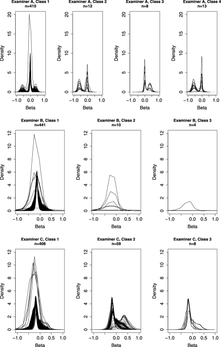
Figure 1: Examiner-specific posterior density estimates of bias parameters ($\beta$’s) for least-squares clusters based on examiner calibration training data.

Based on similarities among posterior density estimates, we collapsed into a single group those sites in classes: 2 and 4 for examiner A; 2 and 3 for examiner B; and 1 and 3 for examiner C. This resulted in posterior clustering inference based on three classes for examiner A, two for examiner B, and two for examiner C (excluding singleton classes). Examiner A’s measures are predominantly unbiased (class 1), but with some evidence of both negative (class 2) and positive (class 3) bias. Examiner B’s measures are overall mildly negatively biased (class 1), but 14 sites in class 2 are cases in which examiner B’s recorded probing depth is 0. In contrast, only 12 of the 441 sites in class 1 are associated with a recording of 0 by examiner B. Examiner C’s measures are overall mildly negatively biased (class 1), but a number of sites are measured with positive bias (class 2).

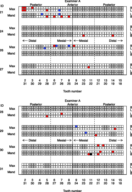
Figure 2: Examiner calibration training exercise examiner A posterior class structure. White${}={}$class 1; Red${}={}$class 2; Blue${}={}$class 3; Black${}={}$Singleton class; Gray${}={}$not observed by examiner. Anterior versus posterior teeth are indicated by the vertical dashed line. For each tooth, the mesial and distal sites are those closest to and furthest from the midline of the dental arch, indicated by the solid vertical line. Abbreviations: Max${}={}$Maxillary; Mand${}={}$Mandibular; B${}={}$Buccal; L${}={}$Lingual.

Figure 2 shows the distribution of class membership across the mouth for sites examined by examiner A [Slate and Hill (2012)]. Using the approach described in Section 2.4.3, for examiner A we observed a significantly larger proportion of: mid-tooth sites in class 2 versus class 1 (64% versus 31%, $p=0.030$); buccal sites in class 2 versus class 1 (68% versus 49%, $p=0.016$); and sites associated with anterior teeth in class 3 versus class 1 (75% versus 49%, $p=0.028$). Recalling for examiner A that class 1 reflects no bias, class 2 reflects negative bias, and class 3 positive bias, we conclude that examiner A is significantly more likely to be negatively biased for mid-tooth and buccal sites and more likely to be positively biased for anterior teeth. Based on similar analyses for examiner B comparing class 2 to class 1, we observe a greater proportion of mid-tooth sites (100% versus 31%) and sites located on mandibular teeth (93% versus 70%, $p=0.052$). Again, recalling for examiner B that class 1 sites are negatively biased, and class 2 sites have recorded depths of 0, we conclude examiner B displays an overall negative bias in measuring behavior relative to the standard, and is more likely to measure a depth of 0 mm for mid-tooth and mandibular sites. For examiner C, there is marginal evidence of a larger proportion of anterior teeth in class 2 versus class 1 (49% versus 24%, $p=0.052$). Recall examiner C’s class 1 and class 2 sites are positively and negatively biased, respectively, relative to the standard. We conclude examiner C’s measures are overall negatively biased, but tend to be positively biased on anterior teeth.

We also examined the relationship between class membership and pocket depth. Specifically, we calculated the median of the posterior distribution of $\theta_{ij}$ and assessed the significance of its association with class membership. Examiner B is significantly more likely to record a probing depth of zero for more shallow sites ($p=0.012$), and examiner C is significantly positively biased for deeper sites ($p=0.0007$).

5 Discussion

In this manuscript we develop a novel approach to inter- and intra-examiner agreement using a semi-parametric Bayesian model with a Dirichlet process prior on model parameters capturing examiner biases, accommodating dependence among measures obtained from the same unit, as well as the dependence between duplicate measures made on the same experimental subunit. At the suggestion of a referee, we fit an alternative model for pocket depth [equation (1)] with an additional tooth-level random effect. We observed modest improvement in fit relative to Model 3 with a reduction in $\mathrm{DIC}_{3}$ ($\Delta\mathrm{DIC}_{3}=13.29$), but there was no meaningful change in posterior inference (results not shown). Recently, a number of authors have demonstrated spatial correlation among measures obtained from periodontal sites within the same mouth, with higher correlation among measures obtained from sites closer together than from those further apart [Reich, Hodges and Carlin (2007)]; we speculate the tooth-level random effect captures some of this spatial heterogeneity. An interesting extension of our approach would investigate improvements in model fit and subsequent inference by specifically modeling spatial correlation among sites in equation (1).

Our analysis has several implications with respect to the design of experiments intended to measure examiner agreement. First, the discovery of sample items where examiners demonstrate greater difficulty with agreement suggests over-sampling within these discovered classes in follow-up calibration studies. Furthermore, it may be possible to reduce the sample sizes needed to determine agreement within specified precision bounds because the model borrows strength across examiner pairs. Finally, we observed in our simulated data set that agreement indices (in particular, $\kappa_{w}$) tend to be smoothed in the direction of the truth. Although our simulation does not permit generalization, this observation is consistent with conclusions made by Guggenmoos-Holzmann and Vonk [Guggenmoos-Holzmann and Vonk (1998)] who show that Cohen’s kappa may be biased when examiners disagree systematically. To mitigate this bias, they suggest using more informative study designs incorporating simultaneous assessment of intra- and inter-examiner variation, a characteristic of the design used in our examiner calibration exercise.

Our approach is not limited to periodontal data applications. For example, a common measure of anti-tumor activity in cancer clinical trials is tumor response, measured on an ordinal scale but derived from a continuous measure of the percentage of tumor shrinkage from baseline in (potentially) multiple target lesions in the same subject [Eisenhauer et al. (2009)]. This endpoint is typically measured by expert reading of CT or MRI scans by trained radiologists. One can envision a calibration exercise in which radiologists are trained to measure response, but scan assessments may be biased based on (for example) tumor location or scan quality. When pooling across examiner pairs is appropriate, our hierarchical model provides refined inference for calibration data that yields greater precision and identification of classes of units measured with similar bias, contributions that enhance the knowledge gained and enable subsequent targeted examiner training.

References

- Albandar, Brunelle and Kingman (1999) {barticle}[pbm] \bauthor\bsnmAlbandar, \bfnmJ. M.\binitsJ. M., \bauthor\bsnmBrunelle, \bfnmJ. A.\binitsJ. A. and \bauthor\bsnmKingman, \bfnmA.\binitsA. (\byear1999). \btitleDestructive periodontal disease in adults 30 years of age and older in the United States, 1988–1994. \bjournalJ. Periodontol. \bvolume70 \bpages13–29. \biddoi=10.1902/jop.1999.70.1.13, issn=0022-3492, pmid=10052767 \bptokimsref \endbibitem
- Brooks and Gelman (1998) {barticle}[mr] \bauthor\bsnmBrooks, \bfnmStephen P.\binitsS. P. and \bauthor\bsnmGelman, \bfnmAndrew\binitsA. (\byear1998). \btitleGeneral methods for monitoring convergence of iterative simulations. \bjournalJ. Comput. Graph. Statist. \bvolume7 \bpages434–455. \biddoi=10.2307/1390675, issn=1061-8600, mr=1665662 \bptokimsref \endbibitem
- Celeux et al. (2006) {barticle}[mr] \bauthor\bsnmCeleux, \bfnmG.\binitsG., \bauthor\bsnmForbes, \bfnmF.\binitsF., \bauthor\bsnmRobert, \bfnmC. P.\binitsC. P. and \bauthor\bsnmTitterington, \bfnmD. M.\binitsD. M. (\byear2006). \btitleDeviance information criteria for missing data models. \bjournalBayesian Anal. \bvolume1 \bpages651–673 (electronic). \biddoi=10.1214/06-BA122, issn=1931-6690, mr=2282197 \bptokimsref \endbibitem
- Cochran (1977) {bbook}[mr] \bauthor\bsnmCochran, \bfnmWilliam G.\binitsW. G. (\byear1977). \btitleSampling Techniques, \bedition3rd ed. \bpublisherWiley, \blocationNew York. \bidmr=0474575 \bptokimsref \endbibitem
- Cohen (1968) {barticle}[pbm] \bauthor\bsnmCohen, \bfnmJ.\binitsJ. (\byear1968). \btitleWeighted kappa: Nominal scale agreement with provision for scaled disagreement or partial credit. \bjournalPsychol. Bull. \bvolume70 \bpages213–220. \bidissn=0033-2909, pmid=19673146 \bptokimsref \endbibitem
- Congdon (2001) {bbook}[mr] \bauthor\bsnmCongdon, \bfnmPeter\binitsP. (\byear2001). \btitleBayesian Statistical Modelling. \bpublisherWiley, \blocationChichester. \bidmr=1852012 \bptokimsref \endbibitem
- Congdon (2007) {barticle}[mr] \bauthor\bsnmCongdon, \bfnmP.\binitsP. (\byear2007). \btitleBayesian modelling strategies for spatially varying regression coefficients: A multivariate perspective for multiple outcomes. \bjournalComput. Statist. Data Anal. \bvolume51 \bpages2586–2601. \biddoi=10.1016/j.csda.2006.01.004, issn=0167-9473, mr=2338990 \bptokimsref \endbibitem
- Dahl (2006) {bincollection}[author] \bauthor\bsnmDahl, \bfnmD B\binitsD. B. (\byear2006). \btitleModel-based clustering for expression data via a Dirichlet process mixture model. In \bbooktitleBayesian Inference for Gene Expression and Proteomics \bpages201–218. \bpublisherCambridge Univ. Press, \baddressNew York. \bptokimsref \endbibitem
- DeRouen, Mancl and Hujoel (1991) {barticle}[pbm] \bauthor\bsnmDeRouen, \bfnmT. A.\binitsT. A., \bauthor\bsnmMancl, \bfnmL.\binitsL. and \bauthor\bsnmHujoel, \bfnmP.\binitsP. (\byear1991). \btitleMeasurement of associations in periodontal diseases using statistical methods for dependent data. \bjournalJ. Periodont. Res. \bvolume26 \bpages218–229. \bidissn=0022-3484, pmid=1831845 \bptokimsref \endbibitem
- Eisenhauer et al. (2009) {barticle}[pbm] \bauthor\bsnmEisenhauer, \bfnmE. A.\binitsE. A., \bauthor\bsnmTherasse, \bfnmP.\binitsP., \bauthor\bsnmBogaerts, \bfnmJ.\binitsJ., \bauthor\bsnmSchwartz, \bfnmL. H.\binitsL. H., \bauthor\bsnmSargent, \bfnmD.\binitsD., \bauthor\bsnmFord, \bfnmR.\binitsR., \bauthor\bsnmDancey, \bfnmJ.\binitsJ., \bauthor\bsnmArbuck, \bfnmS.\binitsS., \bauthor\bsnmGwyther, \bfnmS.\binitsS., \bauthor\bsnmMooney, \bfnmM.\binitsM., \bauthor\bsnmRubinstein, \bfnmL.\binitsL., \bauthor\bsnmShankar, \bfnmL.\binitsL., \bauthor\bsnmDodd, \bfnmL.\binitsL., \bauthor\bsnmKaplan, \bfnmR.\binitsR., \bauthor\bsnmLacombe, \bfnmD.\binitsD. and \bauthor\bsnmVerweij, \bfnmJ.\binitsJ. (\byear2009). \btitleNew response evaluation criteria in solid tumours: Revised RECIST guideline (version 1.1). \bjournalEur. J. Cancer \bvolume45 \bpages228–247. \biddoi=10.1016/j.ejca.2008.10.026, issn=1879-0852, pii=S0959-8049(08)00873-3, pmid=19097774 \bptokimsref \endbibitem
- Escobar and West (1995) {barticle}[mr] \bauthor\bsnmEscobar, \bfnmMichael D.\binitsM. D. and \bauthor\bsnmWest, \bfnmMike\binitsM. (\byear1995). \btitleBayesian density estimation and inference using mixtures. \bjournalJ. Amer. Statist. Assoc. \bvolume90 \bpages577–588. \bidissn=0162-1459, mr=1340510 \bptokimsref \endbibitem
- Escobar and West (1998) {bincollection}[mr] \bauthor\bsnmEscobar, \bfnmMichael D.\binitsM. D. and \bauthor\bsnmWest, \bfnmMike\binitsM. (\byear1998). \btitleComputing nonparametric hierarchical models. In \bbooktitlePractical Nonparametric and Semiparametric Bayesian Statistics \bpages1–22. \bpublisherSpringer, \blocationNew York. \biddoi=10.1007/978-1-4612-1732-9_1, mr=1630073 \bptokimsref \endbibitem
- Fleiss (2001) {bbook}[author] \bauthor\bsnmFleiss, \bfnmJ L\binitsJ. L. (\byear2001). \btitleStatistical Methods for Rates and Proportions. \bpublisherWiley, \blocationNew York. \bptokimsref \endbibitem
- Fleiss et al. (1991) {barticle}[pbm] \bauthor\bsnmFleiss, \bfnmJ. L.\binitsJ. L., \bauthor\bsnmMann, \bfnmJ.\binitsJ., \bauthor\bsnmPaik, \bfnmM.\binitsM., \bauthor\bsnmGoultchin, \bfnmJ.\binitsJ. and \bauthor\bsnmChilton, \bfnmN. W.\binitsN. W. (\byear1991). \btitleA study of inter- and intra-examiner reliability of pocket depth and attachment level. \bjournalJ. Periodont. Res. \bvolume26 \bpages122–128. \bidissn=0022-3484, pmid=1826526 \bptokimsref \endbibitem
- Guggenmoos-Holzmann and Vonk (1998) {barticle}[pbm] \bauthor\bsnmGuggenmoos-Holzmann, \bfnmI.\binitsI. and \bauthor\bsnmVonk, \bfnmR.\binitsR. (\byear1998). \btitleKappa-like indices of observer agreement viewed from a latent class perspective. \bjournalStat. Med. \bvolume17 \bpages797–812. \bidissn=0277-6715, pii=10.1002/(SICI)1097-0258(19980430)17:8¡797::AID-SIM776¿3.0.CO;2-G, pmid=9595612 \bptokimsref \endbibitem
- Hill and Slate (2014) {bmisc}[mr] \bauthor\bsnmHill, \bfnmE. G.\binitsE. G. and \bauthor\bsnmSlate, \bfnmE. H.\binitsE. H. (\byear2014). \bhowpublishedSupplement to “A semi-parametric Bayesian model of inter- and intra-examiner agreement for periodontal probing depth.” DOI:\doiurl10.1214/13-AOAS688SUPP. \bptokimsref \endbibitem
- Hill et al. (2006) {barticle}[pbm] \bauthor\bsnmHill, \bfnmElizabeth G.\binitsE. G., \bauthor\bsnmSlate, \bfnmElizabeth H.\binitsE. H., \bauthor\bsnmWiegand, \bfnmRyan E.\binitsR. E., \bauthor\bsnmGrossi, \bfnmSara G.\binitsS. G. and \bauthor\bsnmSalinas, \bfnmCarlos F.\binitsC. F. (\byear2006). \btitleStudy design for calibration of clinical examiners measuring periodontal parameters. \bjournalJ. Periodontol. \bvolume77 \bpages1129–1141. \biddoi=10.1902/jop.2006.050395, issn=0022-3492, pmid=16805674 \bptokimsref \endbibitem
- Ishwaran and James (2001) {barticle}[mr] \bauthor\bsnmIshwaran, \bfnmHemant\binitsH. and \bauthor\bsnmJames, \bfnmLancelot F.\binitsL. F. (\byear2001). \btitleGibbs sampling methods for stick-breaking priors. \bjournalJ. Amer. Statist. Assoc. \bvolume96 \bpages161–173. \biddoi=10.1198/016214501750332758, issn=0162-1459, mr=1952729 \bptokimsref \endbibitem
- Jones et al. (2006) {barticle}[mr] \bauthor\bsnmJones, \bfnmGalin L.\binitsG. L., \bauthor\bsnmHaran, \bfnmMurali\binitsM., \bauthor\bsnmCaffo, \bfnmBrian S.\binitsB. S. and \bauthor\bsnmNeath, \bfnmRonald\binitsR. (\byear2006). \btitleFixed-width output analysis for Markov chain Monte Carlo. \bjournalJ. Amer. Statist. Assoc. \bvolume101 \bpages1537–1547. \biddoi=10.1198/016214506000000492, issn=0162-1459, mr=2279478 \bptokimsref \endbibitem
- Lunn et al. (2000) {barticle}[author] \bauthor\bsnmLunn, \bfnmD J\binitsD. J., \bauthor\bsnmThomas, \bfnmA\binitsA., \bauthor\bsnmBest, \bfnmN\binitsN. and \bauthor\bsnmSpiegelhalter, \bfnmD\binitsD. (\byear2000). \btitleWinBUGS—A Bayesian modelling framework: Concepts, structure, and extensibility. \bjournalStatist. Comput. \bvolume10 \bpages325–337. \bptokimsref \endbibitem
- Oden (1991) {barticle}[pbm] \bauthor\bsnmOden, \bfnmN. L.\binitsN. L. (\byear1991). \btitleEstimating kappa from binocular data. \bjournalStat. Med. \bvolume10 \bpages1303–1311. \bidissn=0277-6715, pmid=1925161 \bptokimsref \endbibitem
- Osborn et al. (1992) {barticle}[author] \bauthor\bsnmOsborn, \bfnmJ B\binitsJ. B., \bauthor\bsnmStoltenberg, \bfnmJ L\binitsJ. L., \bauthor\bsnmHuso, \bfnmB A\binitsB. A., \bauthor\bsnmAeppli, \bfnmD M\binitsD. M. and \bauthor\bsnmPhilstrom, \bfnmB L\binitsB. L. (\byear1992). \btitleComparison of measurement variability in subjects with moderate periodontitis using a conventional and constant force periodontal probe. \bjournalJ. Periodontol. \bvolume63 \bpages283–289. \bptokimsref \endbibitem
- Reich, Hodges and Carlin (2007) {barticle}[mr] \bauthor\bsnmReich, \bfnmBrian J.\binitsB. J., \bauthor\bsnmHodges, \bfnmJames S.\binitsJ. S. and \bauthor\bsnmCarlin, \bfnmBradley P.\binitsB. P. (\byear2007). \btitleSpatial analyses of periodontal data using conditionally autoregressive priors having two classes of neighbor relations. \bjournalJ. Amer. Statist. Assoc. \bvolume102 \bpages44–55. \biddoi=10.1198/016214506000000753, issn=0162-1459, mr=2345531 \bptokimsref \endbibitem
- Sethuraman (1994) {barticle}[mr] \bauthor\bsnmSethuraman, \bfnmJayaram\binitsJ. (\byear1994). \btitleA constructive definition of Dirichlet priors. \bjournalStatist. Sinica \bvolume4 \bpages639–650. \bidissn=1017-0405, mr=1309433 \bptokimsref \endbibitem
- Slate and Hill (2012) {barticle}[author] \bauthor\bsnmSlate, \bfnmE H\binitsE. H. and \bauthor\bsnmHill, \bfnmE G\binitsE. G. (\byear2012). \btitleDiscovering factors influencing examiner agreement for periodontal measures. \bjournalCommunity Dentistry and Oral Epidemiology \bvolume40 \bpages21–27. \bnoteSuppl. 1. \bptokimsref \endbibitem
- Williamson, Lipsitz and Manatunga (2000) {barticle}[pbm] \bauthor\bsnmWilliamson, \bfnmJ. M.\binitsJ. M., \bauthor\bsnmLipsitz, \bfnmS. R.\binitsS. R. and \bauthor\bsnmManatunga, \bfnmA. K.\binitsA. K. (\byear2000). \btitleModeling kappa for measuring dependent categorical agreement data. \bjournalBiostatistics \bvolume1 \bpages191–202. \biddoi=10.1093/biostatistics/1.2.191, issn=1468-4357, pii=1/2/191, pmid=12933519 \bptokimsref \endbibitem
- Williamson and Manatunga (1997) {barticle}[pbm] \bauthor\bsnmWilliamson, \bfnmJ. M.\binitsJ. M. and \bauthor\bsnmManatunga, \bfnmA. K.\binitsA. K. (\byear1997). \btitleAssessing interrater agreement from dependent data. \bjournalBiometrics \bvolume53 \bpages707–714. \bidissn=0006-341X, pmid=9192459 \bptokimsref \endbibitem