The Kuramoto model of coupled oscillators with a bi-harmonic coupling function

Abstract

We study synchronization in a Kuramoto model of globally coupled phase oscillators with a bi-harmonic coupling function, in the thermodynamic limit of large populations. We develop a method for an analytic solution of self-consistent equations describing uniformly rotating complex order parameters, both for single-branch (one possible state of locked oscillators) and multi-branch (two possible values of locked phases) entrainment. We show that synchronous states coexist with the neutrally linearly stable asynchronous regime. The latter has a finite life time for finite ensembles, this time grows with the ensemble size as a power law.

1 Introduction

Large systems of coupled nonidentical oscillators are of general interest in various branches of science. They describe Josephson junction circuits [1, 2, 3], electrochemical [4] and spin-torque [5, 6] oscillators, as well as variety of interdisciplinary applications including pedestrian induced oscillations of footbridges [7], applauding persons [8], and others. Similar models are also used in biology, for example in studying of neural ensembles dynamics [9, 10] and systems describing circadian clocks in mammals [11, 12]. In many cases the analysis of large ensembles consisting of heterogeneous oscillators can be successfully performed in the phase approximation [13, 14]. Indeed, if the interaction between the elements is weak, the amplitudes are enslaved, and the dynamics of self-sustained oscillators can be effectively described by a relatively simple system of coupled phase equations. The special case of a globally coupled network of phase oscillators (so-called Kuramoto model [13, 15]) attracted a lot of attention [16] and has been established as a paradigmatic model describing transitions from incoherent to synchronous states in the ensembles of coupled oscillators.

Quite a complete analysis of the Kuramoto model can be performed in the case of a harmonic sin-coupling function [13, 17, 18], although even here non-trivial scenaria of transition to synchrony have been reported [19]. Less studied is the case of more general coupling functions, containing many harmonics. Here we perform a systematic study of the synchronous regimes for a bi-harmonic coupling function (see [20] for a short presentation of these results which have been later confirmed in [21]). We introduce the model and discuss previous findings in Section 2. Then in Section 3 we give a general solution of the self-consistent equations describing rotating-wave synchronous solutions. In Section 4 we give a detailed analysis of the simplest symmetric case (no phase shifts in the coupling), while a general situation is illustrated in Section 5. In Conclusion we summarize the results and outline open questions. In this paper we focus on the deterministic oscillator dynamics, the case of noisy oscillators will be considered elsewhere [22].

2 Kuramoto Model and Bi-Harmonic Coupling

The general Kuramoto model is formulated as a system of differential equations for the phases $\phi_{k}$ of $N$ oscillators:

$$\dot{\phi_{k}}=\omega_{k}+\frac{1}{N}\sum_{n=1}^{N}\Gamma(\phi_{n}-\phi_{k}),\qquad k=1,..,N.$$ (1)

All the oscillators are identical, except for diversity of the natural frequencies $\omega_{k}$, distributed according to a certain distribution function $g(\omega)$. The level of coherence in the network of phase oscillators can be essentially described by order parameters $R_{n}$ defined by:

$$R_{n}e^{i\Theta_{n}}=\frac{1}{N}\sum_{k=1}^{N}e^{in\psi_{k}},\ n\in\mathbb{N}.$$

The state with $R_{n}=0$ for all $n$ corresponds to a purely incoherent dynamics (uniform distribution of the phases), while non-zero values of at least some order parameters indicate for certain synchrony in the ensemble. In the case of pure sinusoidal coupling, $\Gamma(x)=\varepsilon\sin(x+\alpha)$, the original analysis by Kuramoto [15, 13] and its subsequent extensions [23, 24, 25, 17, 18] revealed a clear picture of a transition from asynchronous state to coherence in the thermodynamical limit $N\to\infty$. It was shown that above certain critical value of the coupling ($\varepsilon>\varepsilon_{c}$), the system undergoes a transition from disordered behavior to synchronous collective motion via a supercritical bifurcation with the main order parameter obeying $R_{1}\sim(\varepsilon-\varepsilon_{c})^{\frac{1}{2}}$.

The situation is much less trivial for more general coupling functions $\Gamma$. The presence of higher harmonics in coupling function [26, 24, 25, 27] may change scaling of the order parameter to linear law $R_{1}\sim\varepsilon-\varepsilon_{c}$. Moreover, as has been already mentioned in an early paper by Winfree [28] and in subsequent numerical studies by Daido in [29, 30], sufficiently strong higher modes in the coupling function $\Gamma$ may cause a so-called multibranch entrainment, in which a huge number of stable or multistable phase-locked states exists. In certain cases the interplay between synchronizing action of one coupling mode and repelling force from another one can be a reason for an oscillatory behavior of macroscopic order parameters [31].

This paper is devoted to a systematic study of the Kuramoto model in the case of a general bi-harmonic coupling function

$$\Gamma(x)=\varepsilon\sin(x-\beta_{1})+\gamma\sin(2x-\beta_{2})$$ (2)

in the thermodynamic limit $N\to\infty$. In Section 3 we formulate an analytic self-consistent approach [15, 13, 32] which allows us to calculate stationary or uniformly rotating order parameters $R_{1,2}$ (including all possible multi-branch entrainment states) depending on the parameters of the bi-harmonic coupling function $\Gamma$. Based on the self-consistent method, we present in Section 4 a complete diagram of uniformly rotating states with constant order parameters, for a special case of symmetric coupling function $\Gamma$ ($\beta_{1,2}=0$). Surprisingly, (i) synchronous solutions appear prior to the stability threshold of incoherent state; (ii) these regimes have order parameters that can take values anywhere in the range $(0,R_{max}]$ for some $R_{max}<1$; (iii) there is a huge multiplicity of these states for fixed coupling parameters (multi-branch entrainment) which can also appear for relatively weak second mode (when parameter $\gamma$ is small compare to absolute value of $\varepsilon$) in the coupling. Here we also illustrate the multiplicity of solutions, and, combining the self-consistent approach and a perturbative analysis, we derive the scaling laws of $R_{1,2}(\varepsilon,\gamma)$ near the transition points where coherent state appears.

For a general case of non-zero $\beta_{1,2}$, consideration of the self-consistent equations becomes rather tedious due to a large number of parameters involved. We restrict our attention in Section 5 to several examples with multibranch entrainment and to already mentioned oscillatory states [31].

Before proceeding with the analysis, we mention three examples of realistic physical systems where the second harmonics term in the coupling function is strong or even dominating. The first example is the classical Hyugens’ setup with pendulum clocks suspended on a common beam (common platform). The horizontal displacement of the beam leads to the first harmonics coupling $\sim\varepsilon$, while the vertical mode produces the second harmonics term $\sim\gamma$ [33]. We give a derivation of the phase equations for the case where both horizontal and vertical displacements of the platform are present, in Appendix Appendix, where Eq. (29) is in fact the Kuramoto model with bi-harmonic coupling. Another example are recently experimentally realized $\varphi-$Josephson junctions [34], where the dynamics of a single junction in the array is governed by a double-well energy potential. Therefore one can expect strong effects caused by the second harmonics in the interaction. The third example are experiments with globally coupled electrochemical oscillators [35, 36], where a pronounced second harmonics has been observed in the coupling function inferred from the experimental data.

3 Self-consistent equations and their solution

We start our analysis with reformulation of equation (1) for the bi-harmonic coupling as

$$\dot{\varphi}_{k}=\omega_{k}+\varepsilon\text{Im}\left[e^{-i\beta_{1}-i\varphi_{k}}\frac{1}{N}\sum_{n}e^{i\varphi_{n}}\right]+\gamma\text{Im}\left[e^{-i\beta_{2}-i2\varphi_{k}}\frac{1}{N}\sum_{n}e^{i2\varphi_{n}}\right]\;.$$

In the thermodynamical limit, using the two relevant order parameters $R_{1,2}e^{i\Theta_{1,2}}$, we obtain:

$$\dot{\varphi}=\omega+\varepsilon R_{1}\sin(\Theta_{1}-\varphi-\beta_{1})+\gamma R_{2}\sin(\Theta_{2}-2\varphi-\beta_{2})\;.$$ (3)

We assume the natural frequencies $\omega$ to be distributed according to a symmetric, single-maximum function $g(\omega)$. In the thermodynamical limit the complex order parameters $R_{m}e^{i\Theta_{m}}$ can be represented using the conditional distribution function $\rho(\varphi|\omega)$:

$$R_{m}e^{i\Theta_{m}}=\iint d\varphi d\omega\;g(\omega)\rho(\varphi|\omega)e^{im\varphi},\qquad m=1,2\;.$$ (4)

Let us perform a following transformation of variables to the rotating (with some frequency $\Omega$) reference frame:

$$\Theta_{1}=\Omega t+\theta_{1};\ \Theta_{2}=\Omega t+\theta_{2};\ \varphi=\Omega t+\theta_{1}-\beta_{1}+\psi\;.$$ (5)

Then equation (3) changes as follows:

$$\dot{\psi}=\omega-\Omega+\varepsilon R_{1}\sin(-\psi)+\gamma R_{2}\sin(\theta_{2}-2\theta_{1}+2\beta_{1}-\beta_{2}-2\psi)\;.$$ (6)

It is convenient to introduce a set of parameters $\{R,\ u,\ v,\ z\}=\mathbf{P}$ in the following way:

$$\varepsilon R_{1}=R\sin{u},\quad\gamma R_{2}=R\cos{u},\quad\Omega=zR,\quad v=\theta_{2}-2\theta_{1}+2\beta_{1}-\beta_{2}\;.$$ (7)

Now equation (6) takes the form:

$$\dot{\psi}=R\left(x-z-\sin{u}\sin{\psi}-\cos{u}\sin(2\psi-v)\right)=R\left(x-z-y(u,v,\psi)\right)\;.$$ (8)

Here we denoted $x=\omega/R$ and $y(u,v,\psi)=\sin u\sin\psi+\cos u\sin(2\psi-v)$.

Setting parameters $\mathbf{P}$ to some constant values in (8) [this means that $R_{1,2},\theta_{1,2}$ are constants, i.e. the order parameters are uniformly rotating with velocity $\Omega$], one can find a stationary distribution function $\rho(\psi|x,\mathbf{P})$ and then calculate corresponding complex order parameters as:

$$R_{1}e^{i\theta_{1}}=e^{i(\theta_{1}-\beta_{1})}R\iint dxd\psi\rho(\psi|x,\mathbf{P})e^{i\psi}g(Rx)=e^{i(\theta_{1}-\beta_{1})}RF_{1}(\mathbf{P})e^{iQ_{1}(\mathbf{P})}$$ (9)

$$R_{2}e^{i\theta_{2}}=e^{i2(\theta_{1}-\beta_{1})}R\iint dxd\psi\rho(\psi|x,\mathbf{P})e^{i2\psi}g(Rx)=e^{i2(\theta_{1}-\beta_{1})}RF_{2}(\mathbf{P})e^{iQ_{2}(\mathbf{P})}$$

$$F_{m}(\mathbf{P})e^{iQ_{m}(\mathbf{P})}\equiv\iint dxd\psi\rho(\psi|x,\mathbf{P})e^{im\psi}g(Rx)\qquad m=1,2\;.$$

(a) (b)

(c) (d)

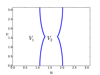
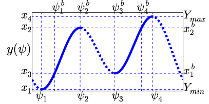
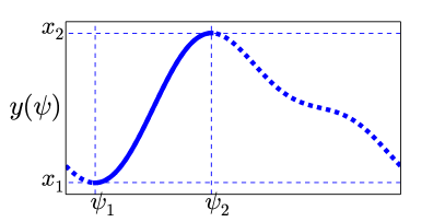
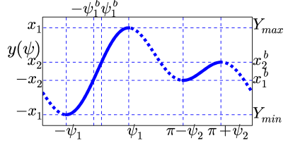
Figure 1: (a) Regions $V_{1}$ and $V_{2}$ in the plane of parameters $(u,v)$: Domain $V_{1}$ corresponds to a double-well form of function $y(u,v,\psi)$ (Fig. 1(b,d)), while in $V_{2}$ $y(u,v,\psi)$ has a single-well form like sown in Fig. 1(c). (b) Example of function $y(u,v,\psi)$ with 4 extrema is presented. There are two stable branches (solid curves) for stationary phases of locked oscillators. The left branch $\psi=\Psi_{1}(x,\mathbf{P})$ is larger than the right one $\psi=\Psi_{2}(x,\mathbf{P})$. $(\psi_{1,2},x_{1,2})$ denote coordinates of the extrema corresponding to the branch $\Psi_{1}$, while $(\psi_{3,4},x_{3,4})$ denotes extrema at $\Psi_{2}$. (c) Example of function $y(u,v,\psi)$ with only two extrema and one stable branch $\psi=\Psi_{1}(x,\mathbf{P})$ (solid curve). (d) Example of function $y(u,v,\psi)$ in the special case $v=0$.

Our next goal is to calculate the integrals $F_{m}(\mathbf{P})$, for this we need to find, using the dynamical equation (8), the distribution function $\rho(\psi|x,\mathbf{P})$. Let $Y_{min}$ and $Y_{max}$ denote the global minimum and the global maximum of function $y(u,v,\psi)$, correspondingly (Fig.1(b)). All the oscillators can be separated into locked ones (for $Y_{max}\geq|x-z|\geq Y_{min}$) or rotating, unlocked ones ($x-z>Y_{max}$ or $x-z<Y_{min}$). The distribution function of rotating oscillators (index $r$) is inversely proportional to their phase velocity:

$$\rho_{r}(\psi|x,\mathbf{P})=g(Rx)\rho(\psi|x,\mathbf{P})=\frac{C(x)}{|x-z-y(\psi,u,v)|}\;,$$ (10)

where $C(x)$ is the normalization constant to which we included also the distribution of frequencies:

$$C(x)=\frac{g(Rx)}{\int_{0}^{2\pi}\frac{d\psi}{|x-z-y|}}.$$

The stationary phases of locked oscillators (index $l$) can be found from the following relation:

$$x-z=y(u,v,\psi)\;.$$ (11)

When finding $\psi$ as a function of $x$, we have to satisfy an additional stability condition $\frac{\partial y(u,v,\psi)}{\partial\psi}>0$ that follows from the dynamical equation (8). In the $(u,v)$ plane there are two regions $V_{1}$ and $V_{2}$ (Fig. 1(a)) which produce qualitatively different properties of system (8) and different types of distribution function $\rho_{l}(\psi|x,\mathbf{P})$:

(i) $\{u,v\}\in V_{1}$

In this case function $y(u,v,\psi)$ has a double-well form like shown in Fig.1(b). According to (11), oscillators can be located on two possible stable branches highlighted by solid curves in Fig.1(b): the first branch is $\psi=\Psi_{1}(x,\mathbf{P})$ in the range $\psi\in[\psi_{1},\psi_{2}]$ and another branch is $\psi=\Psi_{2}(x,\mathbf{P})$ for $\psi\in[\psi_{3},\psi_{4}]$. Here and below we assume $\Psi_{1}(x,\mathbf{P})$ to be the biggest stable branch. In the range $(x-z)\in(x^{b}_{1},x^{b}_{2})$ (Fig. 1(b)) there is an area of bistability on the microscopic level: the oscillators with the same natural frequency $x$ can be locked at two different phases $\Psi_{1}(x,\mathbf{P})$ and $\Psi_{2}(x,\mathbf{P})$. Therefore, the distribution function has the following form:

$$\rho_{l}(\psi|x,\mathbf{P})=\left\{\begin{array}[]{l}(1-S(x))\delta(\psi-\Psi_{1}(x,\mathbf{P}))+S(x)\delta(\psi-\Psi_{2}(x,\mathbf{P}))\\ \text{for $(x-z)\in(x^{b}_{1},x^{b}_{2})$}\\ \delta(\psi-\Psi_{1}(x,\mathbf{P}))\ \ \ \text{for $(x-z)\in[x_{1},x_{2}]\setminus(x_{1}^{b},x_{2}^{b})$}\\ \delta(\psi-\Psi_{2}(x,\mathbf{P}))\ \ \ \text{for $(x-z)\in[x_{3},x_{4}]\setminus(x_{1}^{b},x_{2}^{b})$}\\ \end{array}\right.$$ (12)

Here $0\leq S(x)\leq 1$ is an indicator function describing the redistribution over the stable brunches; this function is arbitrary.

(ii) $\{u,v\}\in V_{2}$

In the second case, function $y(u,v,\psi)$ has only two extrema (Fig. 1(c)) and there is only one stable branch $\psi=\Psi_{1}(x,\mathbf{P})$. The distribution function is:

$$\rho_{l}(\psi|x,\mathbf{P})=\delta(\psi-\Psi_{1}(x,\mathbf{P}))\ \text{for $x\in(z+x_{1},z+x_{2})$}$$ (13)

Taking into account the obtained expressions for the distribution function (10,12,13), the integrals in (9) can be rewritten as follows:

$$F_{m}(\mathbf{P})e^{iQ_{m}(\mathbf{P})}=\int_{\psi_{1}}^{\psi_{2}}d\psi e^{im\psi}g\left(R(z+y)\right)\frac{\partial y}{\partial\psi}-$$ (14)

$$\int_{\psi^{b}_{1}}^{\psi^{b}_{2}}d\psi e^{im\psi}S(z+y)g\left(R(z+y)\right)\frac{\partial y}{\partial\psi}+\int_{\psi_{3}}^{\psi_{4}}d\psi e^{im\psi}g\left(R(z+y)\right)\frac{\partial y}{\partial\psi}-$$

$$\int_{\psi^{b}_{3}}^{\psi^{b}_{4}}d\psi e^{im\psi}\left(1-S(z+y)\right)g\left(R(z+y)\right)\frac{\partial y}{\partial\psi}+\int_{\mathcal{X}}\int_{0}^{2\pi}dxd\psi\frac{C(x)e^{im\psi}}{|x-z-y|}$$

Here in the last integral we denote the interval $\mathcal{X}=(-\infty,z+Y_{min})\bigcup(z+Y_{max},\infty)$.

Now, using the integrals (14), one can calculate the absolute values of the complex order parameters $R_{1,2}$ and the frequency $\Omega$ as functions of introduced parameters $R$, $u$, $v$, $z$:

$$R_{1,2}(\mathbf{P})=RF_{1,2}(\mathbf{P}),\ \Omega(\mathbf{P})=Rz\;.$$ (15)

Then, from relations (7), (9) and (15) it follows that:

$$\varepsilon(\mathbf{P})=\frac{\sin{u}}{F_{1}(\mathbf{P})},\ \gamma(\mathbf{P})=\frac{\cos{u}}{F_{2}(\mathbf{P})},\ \beta_{1}(\mathbf{P})=Q_{1}(\mathbf{P}),\ \beta_{2}(\mathbf{P})=Q_{2}(\mathbf{P})-v\;.$$ (16)

All together equations (15) and (16) determine the stationary amplitudes of the order parameters $R_{1,2}$ and the frequency of their rotation $\Omega$ in dependence on model parameters $\varepsilon$, $\gamma$, $\beta_{1,2}$ in an analytic, albeit parametric form. Note that this solution fully accounts to multi-branch entrainment, due to presence of the indicator function $S$. Arbitrariness of this functions means that there is a huge multiplicity of microstates.

We stress, that in the solution (15,16) parameters $R$, $u$, $v$, $z$ and the indicator function are independent, while the order parameters $R_{1,2}$ and the coupling parameters $\varepsilon,\gamma,\beta_{1,2}$ are functions of them. If, on the other hand, one wants to fix the coupling parameters, then one should adjust some of the parameters $R$, $u$, $v$, $z$ and the indicator function, which will be now not independent. This is a standard procedure in a parametric representation of a solution.

4 Symmetric bi-harmonic coupling function

Here we consider the simplest case where $\beta_{1}=\beta_{2}=0$, what corresponds to a symmetric coupling function $\Gamma(x)=\varepsilon\sin(x)+\gamma\sin(2x)$.

4.1 General solution of self-consistent equations

Due to the symmetry of the coupling function, it is possible to perform the self-consistent approach in the special case $z=v=0$ (see however Section 4.7 for a more general situation). First we will simplify equations (14,15,16) taking into account the relation $z=v=0$.

A typical form of function $y(u,v=0,\psi)$ is presented in Fig. 1(d). For $v=0$, the critical value $u=\pm\arctan(2)$ separates double-well and single-well shapes of function $y(u,0,\psi)$. If $|\tan(u)|<2$, the function $y(u,0,\psi)$ contains two stable branches $\Psi_{1}$ and $\Psi_{2}$ (see Fig. 1(d)), otherwise only one branch $\Psi_{1}$ exists like it is shown in Fig. 1(c). The stable branches $\Psi_{1}$ and $\Psi_{2}$ (if exists) are always centered in the intervals

$$\Psi_{1}:\ [-\psi_{1},+\psi_{2}]\ \text{and}\ \Psi_{2}:[\pi-\psi_{2},\pi+\psi_{2}],$$

where the values $\psi_{1,2}$ can be calculated explicitly:

$$\psi_{1,2}=\arccos\left(\frac{\mp\sin u+\sqrt{\sin^{2}u+32\cos^{2}u}}{8\cos u}\right)$$

Moreover, the branches $\Psi_{1,2}$ are symmetric (see Fig.1(d)):

$$y(u,0,\psi)=-y(u,0,-\psi),\ y(u,0,\pi+\psi)=-y(u,0,\pi-\psi).$$

Taking all this into account, the relations (14) can be radically simplified:

$$F_{m}(R,u)e^{iQ_{m}(R,u)}=\int_{-\psi_{1}}^{\psi_{1}}d\psi e^{im\psi}S(y)g\left(R(y)\right)\frac{\partial y}{\partial\psi}+$$ (17)

$$\int_{\pi-\psi_{2}}^{\pi+\psi_{2}}d\psi e^{im\psi}(1-S(y))g\left(R(y)\right)\frac{\partial y}{\partial\psi}+\int_{|x|>x_{1}}\int_{0}^{2\pi}dxd\psi\frac{C(x)e^{im\psi}}{|x-z-y|}\;.$$

Here we assumed that $S(y)=1$ everywhere outside interval $[-\psi_{2},\psi_{2}]$ (see Fig. 1). If the functions $S(x)$ and $g(x)$ are even, then it is easy to see that the imaginary part in all of the integrals in (17) vanishes (recall that $y(u,0,\psi)$ is odd). Thus, for any $S(x)=S(-x)$ and $g(x)=g(-x)$ we obtain $Q_{1,2}(R,u)=0$ and automatically $\beta_{1,2}=0$. (See Section 4.7 below for discussion of an asymmetric indicator function $S$.)

In summary, for the case $z=v=0$ and even $S(x)$, $g(x)$ we have $\Omega=\beta_{1,2}=0$ and the following expressions for the parameters $\varepsilon,\gamma$ and real order parameters $R_{1,2}$ as functions of two introduced parameters $R,u$:

$$R_{1,2}(R,u)=RF_{1,2}(R,u),\ \varepsilon(R,u)=\frac{\sin{u}}{F_{1}(R,u)},\ \gamma(R,u)=\frac{\cos{u}}{F_{2}(R,u)}.$$ (18)

4.2 Stability of the incoherent state

(a) (b)

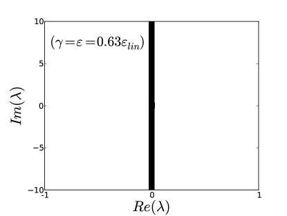
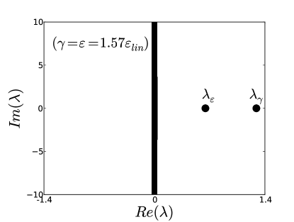
Figure 2: Illustration of the spectra of incoherent state in two different regions: (a) continuous part of the spectrum lies on the imaginary axes revealing neutral stability in the region $\gamma<\gamma_{lin}$, $\varepsilon<\varepsilon_{lin}$, (b) when on of the couplings exceeds threshold $\varepsilon>\varepsilon_{lin}$ or $\gamma>\gamma_{lin}$ the eigenvalue with positive real part appears in the discrete part of the spectrum. Both calculation were made for the Gaussian distribution of frequencies $g(\omega)=\frac{1}{2\pi}e^{-\omega^{2}/2}$, $\varepsilon_{lin}=\gamma_{lin}=2\sqrt{\frac{2}{\pi}}$.

Before proceeding with presentation of the main results we recall that an issue of linear stability of the incoherent state (with uniform distribution of phases) was a milestone in almost all preceding mathematical studies [37, 24, 25, 27] of Kuramoto-type models. This analysis of the partial differential equation for the density distribution function revealed the following stability properties of the incoherent state [37, 24, 25, 27]: (i) the continuous part of the spectrum always lies on the imaginary axis; (ii) when one of the couplings exceeds certain threshold $\varepsilon>\varepsilon_{lin}$ or $\gamma>\gamma_{lin}$, in the discrete spectrum appears an eigenvalue ($\lambda_{\varepsilon}$ or $\lambda_{\gamma}$ correspondingly) with a positive real part revealing instability of the asynchronous state. We illustrate this in Fig. 2. In the linear theory, the modes of the perturbation corresponding to the harmonics of the coupling are independent on each other, and one gets $\varepsilon_{lin}=\gamma_{lin}=\frac{2}{\pi g(0)}$. Below in this paper we use a Gaussian distribution of frequencies $g(\omega)=(2\pi)^{-1/2}\exp(-\omega^{2}/2)$, thus $\varepsilon_{lin}=\gamma_{lin}=2\sqrt{\frac{2}{\pi}}$. In presentation of the results, we will always normalize the values of the coupling parameters $\varepsilon,\gamma$ by the linear stability thresholds.

4.3 Diagram of synchronous states

(a) (b)

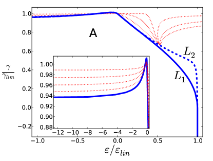
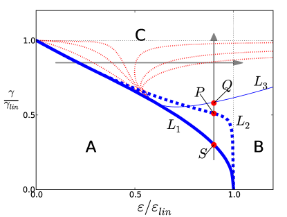
Figure 3: (a) Diagram of different synchronous states in dependence on parameters $(\varepsilon,\gamma)$, resulting from the analytical solution Eqs. (17,18). Bold (blue) line $L_{1}$: border of synchronous states, inside area A there is only the incoherent solution; bold dashed (blue) line $L_{2}$: order parameters vanish. Between lines $L_{1}$ and $L_{2}$ there are two solutions (stable and unstable) with non-zero $R_{1,2}$ and the transition to synchrony is hard (see region between points $S$ and $P$ in Fig. 4(a)). Dotted (red) lines: onset of synchrony for $\sigma=0.2,\,0.4,\,0.5,\,0.6,\,0.8,\,1$ (from left to right). Inset shows the domain $\varepsilon<0$ in more details (with the same axes). (b) The same as in Fig. 3(a) but in the area $\varepsilon,\ \gamma>0$. An additional line $L_{3}$ is drawn from the condition $\tan u=2$, dividing domains B (single synchronous state) and C (multiple synchronous states). Above $L_{3}$ multiplicity of synchronous states due to multi-branch entrainment occurs (beyond point $Q$ in Fig. 4(a)).

(a) (b)

(c) (d)

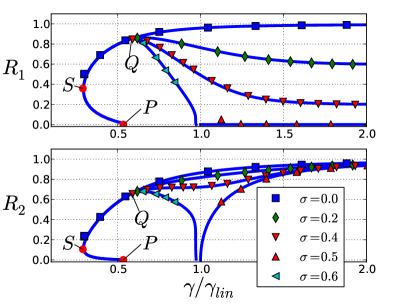
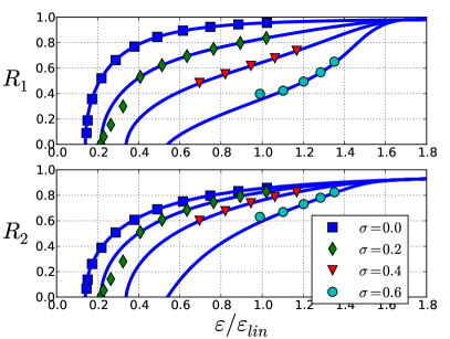
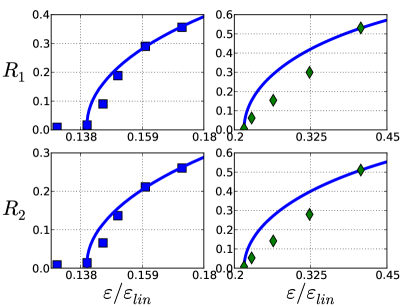
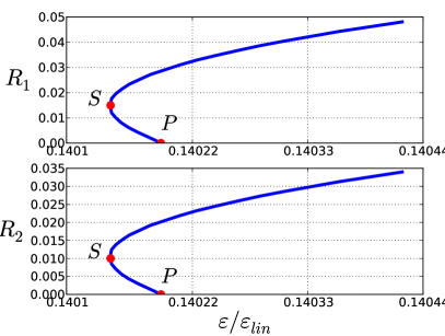
Figure 4: (a) Dependence of the order parameters $R_{1,2}$ on coupling strength $\gamma$ at fixed value of $\varepsilon=0.9\varepsilon_{lin}$ (see also vertical arrow in Fig. 3(b)). Markers are results of direct simulation of a population of $N=2\cdot 10^{4}$ oscillators. Different curves correspond to different values of $\sigma$, as depicted on the panel. For $\gamma\lesssim 0.6\gamma_{\text{lin}}$ there is a unique synchrony state, for larger couplings multiplicity is observed. Point $S$ denotes a “saddle-node bifurcation” at which coherent states appear (curve $L_{1}$ in Fig. 3). At point $P$ the order parameters at the unstable branch of coherent solution vanish (curve $L_{2}$ in Fig. 3). Between points $S$ and $P$ a finite perturbation of the incoherent state is needed to come to a synchronous regime. Point $Q$, the onset of multiplicity, corresponds to curve $L_{3}$ in Fig. 3(b). (b) The same as in Fig. 4(a) but for $\gamma=0.9\gamma_{lin}$, and varying $\varepsilon$. For $\varepsilon\gtrsim 1.6\varepsilon_{\text{lin}}$ the solution is unique, for smaller $\varepsilon$ there are multiple states with different $\sigma$ appearing at different critical couplings. (c) Detailed view of curves $R_{1,2}(\varepsilon)$ for $\sigma=0$ (left panels) and $\sigma=0.2$ (right panels). For both cases $\gamma=0.9\gamma_{lin}$. Here markers denote averaged values of stationary order parameters of different independent numerical simulations (see text). (d) Enlargement of the curves $R_{1,2}(\varepsilon)$ ($\sigma=0$, $\gamma=0.9\gamma_{lin}$, panel(b)) for small values of order parameters, indicating a first-order type of the transition hardly seen in (b).

In Figs. 3 we illustrate the diagram of the states on the plane of parameters $(\varepsilon,\gamma)$, and in Fig. 4 some cuts of it, for the simplest case, where the indicator function $S(\omega)=\sigma$ is a constant. This diagram is obtained by application of analytic formulas (18).

We start the description with an even simpler case $\sigma=0$ (so that all the phases are on one stable branch). Setting in (17),(18) $R=0^{+}$ and varying $u$, we find a curve on the plane of parameters $(\varepsilon,\gamma)$ where the order parameters $R_{1,2}$ vanish (line $L_{2}$ in Fig. 3, see Section 4.8 below for the details of calculation of this line). Remarkably, solutions $R_{1,2}(\varepsilon,\gamma)$ behavior characteristic for first-order phase transitions, as the coupling strengths $(\varepsilon,\gamma)$ increase (Fig. 4a; exception are the pure cases $\varepsilon=0$ and $\gamma=0$, see Section 4.8 below). Therefore, in the plane $(\varepsilon,\gamma)$ also exists the curve $L_{1}$ which corresponds to the line of a “saddle-node bifurcation” where two branches of coherent solutions first appear (point $S$ in Fig. 4a). This line $L_{1}$ split the plane $(\varepsilon,\gamma)$ in two different regions: in area $A$ in Fig. 3(a,b) only incoherent solution of self-consistent equations exists, outside area $A$ (regions $B$ and $C$ in Fig. 3(b)) synchronous solution(s) exist. Between curves $L_{1}$ and $L_{2}$ there are two solutions with $\sigma=0$. We also show a curve $L_{3}$ corresponding to the parameter value $\tan u=2$, which separates the two-branch (Fig. 1(a,d)) and the one-branch (Fig. 1(b)) situations (marked as C and B on panel Fig. 3(b) correspondingly).

Below $L_{3}$ there is a solution with $S(\omega)=0$ only, above it, multiplicity due to arbitrariness of the indicator function $S(\omega)$ occurs. We depict also curves corresponding to synchronous solutions with $R_{1,2}=0^{+}$ at several fixed values of $\sigma$ (red curves in Fig. 3), to the right of these curves synchronous states with corresponding values of $\sigma$ exist.

We illustrate different synchronous regimes as functions of coupling parameters $(\varepsilon,\gamma)$ in Figs. 4(a,b). Fig. 4(a) shows dependence of synchronous states on the coupling parameter $\gamma$ for fixed $\varepsilon=0.9\varepsilon_{\text{lin}}$ (vertical arrow in Fig. 3(b)). As it has been mentioned above, two branches of coherent solutions arise at point $S$. With increase of $\gamma$, the lower branch merge with incoherent solution at point $P$. The upper branch is unique until the border of multiplicity $\tan u=2$ (point $Q$) is crossed. Multiple solutions exist for all larger values of $\gamma$.

A special symmetric solution appears at the linear threshold $\gamma=\gamma_{lin}$. This regime contains only the second harmonic ($R_{1}=0$) and has symmetric redistribution of oscillators ($\sigma=0.5$) between the two symmetric stable branches. This regime appears as a square root of supercriticality $R_{2}\sim(\gamma-\gamma_{c})^{\frac{1}{2}}$ (see the branch of $R_{2}$ starting at $\gamma/\gamma_{lin}=1$ for $\sigma=0.5$ in Fig. 4(a)) and corresponds to the bifurcation from the asynchronous state as described in [24, 25].

In Fig. 4(b) the order parameters are shown as functions of $\varepsilon$ for fixed $\gamma=0.9\gamma_{lin}$(horizontal arrow in Fig. 3(b)). As here almost everywhere we are in the region of multiplicity, the synchrony arises at different values of $\varepsilon$ for different $\sigma$, and immediately beyond the threshold (which corresponds to $\sigma=0$) multiple synchrony states with $\sigma>0$ are possible (as here $\tan u<2$). With further increase of $\varepsilon$, when the line $L_{3}$ is crossed (at large values of $\varepsilon$ not shown in Fig. 3(b)), multiplicity disappears.

In contrast to Fig. 4(a), the first synchronous solution $\sigma=0$ in Fig. 4(b) looks like arising via a second-order phase transition. However a detailed analysis of the situation in Fig. 4(d) shows that it is not the case (as was erroneously stated in [20]). With decrease of parameter $u$ to zero (decrease of $\varepsilon$), lines $L_{1}$ and $L_{2}$ come close to each other but they merge only in the point $u=0$ which corresponds to the pure second-harmonics Kuramoto model ($\varepsilon=0$). In the Section 4.8 below, using a combination of the self-consistent approach and of a perturbative analysis, we will show that at $L_{2}$ the dependence of $R_{1,2}$ on coupling strengths $\varepsilon$ and $\gamma$ is linear with negative slope, everywhere except singular points $u=0$ and $u=\pi/2$ which correspond to the pure cases of second-harmonic and first-harmonic Kuramoto models, respectively.

4.4 Stability properties

Unfortunately, we cannot perform analytically, and even numerically, a thorough stability analysis of the constructed solutions. The only analytic results we can rely on, are outlined in Section 4.2 stability calculations of the asynchronous state $R_{1,2}=0$, yielding instability for $\varepsilon>\varepsilon_{\text{lin}}$ or $\gamma>\gamma_{\text{lin}}$, and neutral stability due to a continuous spectrum otherwise [37, 24, 25, 27]. This conclusion can be easily reproduced numerically, see Fig. 2. However, we could not study in the same manner stability of found self- consistent solutions, because these solutions have a singular component (delta-function in Eqs. (12,13)).

Therefore, we checked for stability via direct numerical simulation of large ensembles (see also [21]). They follow the theoretically predicted curves, as show markers in Figs. 4(a,b). At low values of $R_{1,2}$ these solutions however can be hardly confirmed due to finite-size effects.

In order to study these finite-size effects in the vicinity of “bifurcation points”, i.e. for small values of the order parameters, we performed additional simulations with large ensemble size $N=2^{18}=262144$. Two theoretical curves with $\sigma=0$ and $\sigma=0.2$ for $\gamma=0.9\gamma_{lin}$ (Fig. 4(b)) have been tested for stability. In each simulation we independently generated random distribution of frequencies for $N=262144$ oscillators and prepared initial conditions according to the distribution function, obtained from our self-consistent analysis at given parameters. As a result, Fig. 4(c) shows the averaged values of $R_{1,2}$ (obtained from the numerical simulation of more than 32 independent runs for each point). One can see that the markers are slightly below the curves, indicating that on average synchronization is weaker than the analytically predicted level. Nevertheless, certain level of coherence is always present and it is in a reasonable agreement with analytically predicted curves.

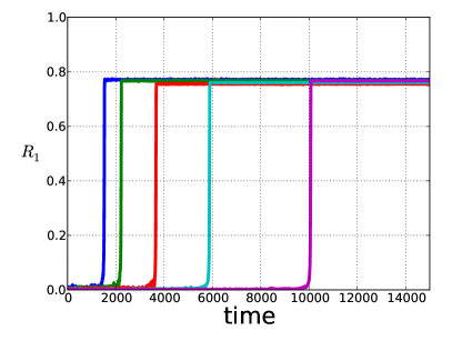
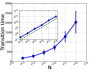
Figure 5: (a) Examples of time evolution of the order parameter $R_{1}$ in direct simulations of an ensemble (1) for $\gamma=0.85\gamma_{lin},\varepsilon=0.6\varepsilon_{lin}$ and different $N$ (from left to right, $N=5\cdot 10^{4},10^{5},2\cdot 10^{5},5\cdot 10^{5},10^{6}$). (b) Averaged transition times from the incoherent state to a synchronous solution, in dependence on the ensemble size $N$ for $\gamma=0.85\gamma_{lin}$, $\varepsilon=0.6\varepsilon_{lin}$. Error bars show standard deviations. Each point was obtained from a statistics of 128 different simulations. Inset shows the same plot in log-log scale. One can see a power low with exponent $\approx 0.7151$.

Next, we simulated the linearly neutrally stable asynchronous state, in the region beyond the curve $L_{2}$, where also synchronous solutions exist. In simulations this state appears to be only metastable. After a transient, which becomes longer for very large ensembles, the ensemble evolves abruptly to one of the synchronous states, we illustrate this in the Fig. 5(a). Remarkably, the averaged time that the system spends in the vicinity of incoherent metastable state grows as a power low of number of oscillators $N$ (Fig. 5(b)).

Thus, although the curves in Fig. 4(b) look like for a standard hysteretic transition, it is not the case: on line $L_{2}$ (at point $P$) the incoherent steady state does not become linearly unstable, instead it remains linearly neutrally stable in the thermodynamic limit, but is metastable due to finite-size effects. This neutral stability/metastability allows also synchronous states to appear with arbitrary small amplitudes $R_{1,2}$ (see on Fig. 3(a,b) curve $L_{2}$ and corresponding curves for different values of $\sigma$, which occupy the whole region on this diagram, and also Fig. 4(b)). Therefore, the points in Fig. 4(b) where $R_{1,2}$ vanish, do not correspond to a usual bifurcation from an equilibrium, and cannot be described as the points where the incoherent state becomes linearly unstable. While this issue requires further investigation, we attribute it to singularity of the appearing states: as one can see from Eq. (12),(13), the density includes a combination of delta-functions for any small $R_{1,2}$, similar to the Van Kampen modes in plasmas [38], while in the stability analysis [24, 25] one operates with modes which apparently cannot straightforwardly describe constructed singular solutions.

4.5 Illustration of multi-branch entrainment states

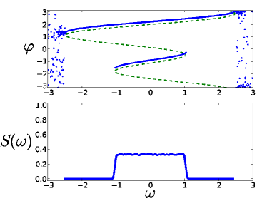
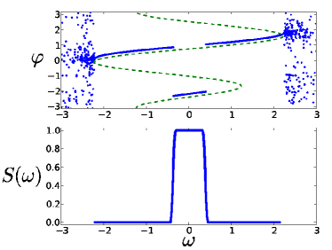
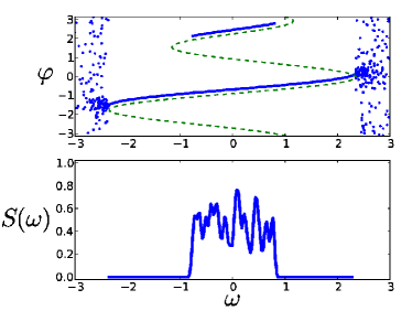
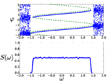
Figure 6: Illustration of multiplicity of states ($\varepsilon=\gamma=1.25\varepsilon_{\text{lin}}$, $N=2\cdot 10^{4}$). In all cases one can see two stable branches of locked phases and the corresponding coarse-grained indicator function $S(\omega)$.

Here we discuss the issue of multiplicity and illustrate different multi-branch entrainment states [29, 30]. As mentioned above, in the thermodynamic limit any indicator function $S(x)$ admittable, so that for fixed parameters $\varepsilon,\gamma$, to a macro-state with given order parameters $\varepsilon,\gamma,R_{1,2}$ belong many micro-states with different redistributions between the stable branches. In Fig. 6 we show several multi-branch states for a certain choice of coupling parameters. If both branches are occupied, one observes a two-hump distribution of locked phases which can be also interpreted as a two-cluster state (cf. [35]).

In fact, we can easily estimate the degree of the multiplicity. We can view the locked oscillators in the bistability range as “uncoupled spins”. Assuming for simplicity that the phases of two branches differ by $\pi$, we conclude that the order parameter $R_{2}$ does not depend on the “spin orientation”, i.e. on which branch they are sitting, while $R_{1}$ can be interpreted as a “magnetization”. Then finding the number of different micro-states at prescribed values of the order parameters reduces to a textbook problem of calculating the entropy

$$\mathcal{S}(R_{1})=N_{\text{bist}}\left[-\left(\frac{1-R_{1}}{2}\right)\ln\left(\frac{1-R_{1}}{2}\right)-\left(\frac{1+R_{1}}{2}\right)\ln\left(\frac{1+R_{1}}{2}\right)\right]$$

for a constant magnetization for $N_{\text{bist}}$ non-interacting spins (the latter is the number of locked oscillators in the range of bistability; it is less than $N$ but is a macroscopic quantity for $R_{1,2}$ not too small). Correspondingly, the number of micro-states grows exponentially with the number of locked oscillators $\sim e^{\mathcal{S}(R_{1})}$ (cf. [30]).

4.6 Competition of the coupling terms

(a)

(b) (c)

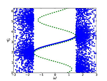
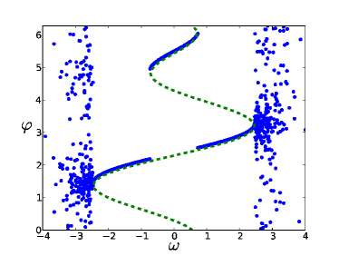
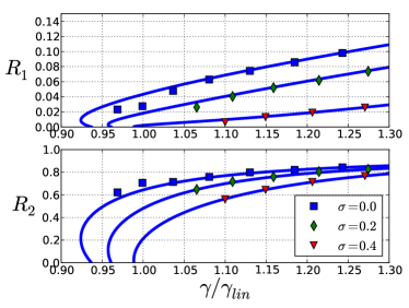
Figure 7: (a) Dependence of order parameters $R_{1,2}$ on coupling strength $\gamma$ at $\varepsilon=-9.29\gamma_{lin}$. (b,c) Phases of oscillators versus internal frequencies are plotted. For both cases $\gamma=1.18\gamma_{lin}$. In the plot (a) $\varepsilon=0.16\varepsilon_{lin}$, in (b) $\varepsilon=-9.29\varepsilon_{lin}$. Markers are result of direct simulation for $N=2\times 10^{4}$.

A non-trivial consequence of the multi-branch entrainment occurs in the region of negative $\varepsilon$. When $\varepsilon<0$, the coupling due to the first mode in the coupling function is repulsive (or desynchronizing); it tends to stabilize the incoherent state and to destroy synchrony. With the second harmonic in coupling function, one might expect that the repulsion for large negative $\varepsilon$ should be compensated by a strong attractive second-harmonic coupling with large positive $\gamma$, for synchronization in the system to occur. However, following the curve $L_{1}$ in Fig. 3(a) one can see that the critical value of $\gamma$ decreases and tends to some constant value below $\gamma_{\text{lin}}$ as $\varepsilon\to-\infty$. This means that the effect of very strong repulsive coupling via the first harmonic can be compensated by a relatively weak synchronizing force $\sim\gamma$. Figure 7(a) shows dependencies $R_{1,2}(\gamma)$ at $\varepsilon=-9.29\varepsilon_{lin}$. Remarkably, the presented solutions are characterized by rather low values of $R_{1}$. The plots of $\phi(\omega)$ in Fig. 7(b,c) shed light onto this effect. In the region $\varepsilon>0$ the solutions appearing on the line $L_{1}$ have simple structure of single-branch entrainment states (Fig. 7(b)). On the contrary, in the region of repulsing first-harmonic coupling $\varepsilon<0$, the appearing solutions represent two-cluster states with indicator function $S=1$, like in Fig. 7(c). The oscillators are distributed among the branches in such a way that the value of $R_{1}$ is minimal, so that effective repulsive force $\varepsilon R_{1}$ (see eq.(3)) is sufficiently weak.

4.7 Non-symmetric solutions

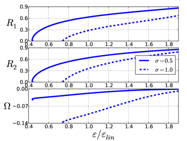
Until now we considered the cases where the functions $S(x)$ (indicator function) and $g(x)$ (distribution of frequencies) were even $S(x)=S(-x)$, $g(x)=g(-x)$. Such symmetric indicator and frequency distribution functions yield solutions with $\beta_{1,2}=0$ and $\Omega=0$ at zero values of parameters $z=v=0$ in the self-consistent equations (14,15,16). However in the general case of non-even $S(x)$ or $g(x)$ zero values of $\beta_{1,2}$ correspond to certain non-zero $z$ and $v$. For example, asymmetric redistribution of oscillators between stable branches (a non-even indicator function $S(x)\neq S(-x)$) gives rise to a non-zero frequency shift $\Omega=Rz\neq 0$ even in the case of $\beta_{1,2}=0$ and symmetric distribution of frequencies $g$. The example is presented in the figure 8 where we use $S(x)=\sigma$ for $x<(x^{b}_{1}+x^{b}_{2})/2$ (see Fig. 1(b)) and $S(x)=0$ otherwise.

Figure 8: Dependence of the order parameters $R_{1,2}$ and their frequency $\Omega$ on coupling strength $\varepsilon$ at $\gamma=0.9\gamma_{lin}$ and $\beta_{1,2}=0$ for non-even indicator function: $S(x)=\sigma$ for $x<(x^{b}_{1}+x^{b}_{2})/2$ (see Fig. 1(b)) and $S(x)=0$ otherwise.

4.8 Perturbative analysis near critical points

In this section we combine the self-consistent approach (17,18) with a perturbative analysis, to derive the scaling law of macroscopic order parameters in the vicinity of bifurcation line $L_{2}$ (Fig. 3) where coherent solution appears. The idea is to consider (17,18) in the limit $R\to 0$ and to find dependence of $R_{1,2}$ on criticalities $(\varepsilon-\varepsilon_{c})$ and $(\gamma-\gamma_{c})$ in this limit of vanishing order parameters. For simplicity of presentation we will assume below $S(x)=0$ (all oscillators are on the same branch and $\varepsilon_{c}$, $\gamma_{c}$ are on the curve $L_{2}$) and shortly discuss other possibilities at the end of this section. In this case (17) reads

$$F_{m} =\int_{0}^{2\pi}d\psi\cos m\psi g(Ry)\frac{\partial y}{\partial\psi}+\int_{0}^{2\pi}\int_{|x|>x_{1}}^{\pm\infty}dxd\psi\frac{g(Rx)C^{\prime}(x)\cos(m\psi)}{|x-y(u,\psi)|}$$

$$\equiv A_{m}(R,u)+B_{m}(R,u)\;,\qquad m=1,2\;.$$

(Here $C^{\prime}$ is the normalization constant). Because $g(x)$ is a symmetric one-hump function, its expansion for small arguments reads $g(x)=g(0)-G_{2}x^{2}+\ldots$. Suppose that $R\ll 1$, than the first term in equation for $F_{m}$ can be represented using this series for $g$ as follows:

$$A_{m}=\int_{0}^{2\pi}d\psi\cos m\psi(g(0)-G_{2}R^{2}y^{2})\frac{\partial y}{\partial\psi}=A_{m0}-A_{m2}R^{2}\;.$$ (19)

For calculation of the second term $B_{m}$ we first compute

$$\Phi_{m}(x)=\frac{\int_{0}^{2\pi}\frac{d\psi\cos(m\psi)}{|x-y(u,\psi)|}}{\int_{0}^{2\pi}\frac{d\psi}{|x-y(u,\psi)|}}$$

With notation $z=1/x$ we get

$$\Phi_{m}(z)=\frac{\int_{0}^{2\pi}\frac{d\psi\cos(m\psi)}{|1-zy(u,\psi)|}}{\int_{0}^{2\pi}\frac{d\psi}{|1-zy(u,\psi)|}}$$

$$=\frac{\int_{0}^{2\pi}d\psi\cos(m\psi)[1+zy(u,\psi)+z^{2}y^{2}(u,\psi)+\ldots]}{\int_{0}^{2\pi}d\psi[1+zy(u,\psi)+z^{2}y^{2}(u,\psi)+\ldots]}\;.$$

Substituting here expression for $y$ we get

$$\Phi_{1}(z)=\frac{z^{2}\pi\sin u\cos u}{2\pi+z^{2}\pi}\approx z^{2}\frac{1}{2}\sin u\cos u=z^{2}\Phi_{12}\;,$$

$$\Phi_{2}(z)=\frac{z^{2}\pi(-\sin^{2}u/2}{2\pi+z^{2}\pi}\approx-z^{2}\frac{1}{4}\sin^{2}u=z^{2}\Phi_{22}\;,$$

or in the old notation

$$\Phi_{1}(x)=x^{-2}\Phi_{12},\quad\Phi_{2}(x)=x^{-2}\Phi_{22},\quad\Phi_{12}=\frac{\sin u\cos u}{2},\quad\Phi_{22}=-\frac{\sin^{2}u}{4}\;.$$ (20)

The last expressions are valid for $x\gg 1$. For small $x$, $\Phi_{m}$ are bounded from above $\Phi_{m}(x)\leq\bar{\Phi}_{m}$.

Now we can rewrite the integrals in the expression for $B_{m}$ as

$$B_{m}=\int_{|x|>x_{1}}^{\pm\infty}dxg(Rx)\Phi_{m}(x)=2\int_{x_{1}}^{\infty}dxg(Rx)\Phi_{m}(x)=$$

$$=2\int_{x_{1}}^{\infty}dxg(0)\Phi_{m}(x)+2\int_{x_{1}}^{\infty}dx[g(Rx)-g(0)]\Phi_{m}(x)\equiv B_{m0}-\tilde{B}_{m}\;.$$

To calculate the last term, we divide the integration range into two subintervals

$$\tilde{B}_{m} =2\int_{x_{1}}^{\infty}dx[g(0)-g(Rx)]\Phi_{m}(x)$$

$$=2\int_{x_{1}}^{R^{-1/6}}dx[g(0)-g(Rx)]\Phi_{m}(x)+2\int_{R^{-1/6}}^{\infty}dx[g(0)-g(Rx)]\Phi_{m}(x)$$

In the first interval we use the upper bound for $\Phi_{m}$, and because here $Rx\ll 1$, we use the expansion $g(x)=g(0)-G_{2}x^{2}$:

$$2\int_{x_{1}}^{R^{-1/6}}dx[g(0)-g(Rx)]\Phi_{m}(x)<2\bar{\Phi}_{m}G_{2}R^{2}\int_{x_{1}}^{R^{-1/6}}x^{2}dx=$$

$$2/3\bar{\Phi}_{m}G_{2}R^{2}(R^{-1/2}-x_{1}^{3})=\mathcal{O}(R^{3/2})$$

In the second integral, because $x\gg 1$, we use the expansion (20) for $\Phi_{m}(x)$

$$2\int_{R^{-1/6}}^{\infty}dx[g(0)-g(Rx)]\Phi_{m}(x)=2\Phi_{m2}\int_{R^{-1/6}}^{\infty}dx[g(0)-g(Rx)]x^{-2}=$$

$$=2\Phi_{m2}R\int_{R^{5/6}}^{\infty}dz[g(0)-g(z)]z^{-2}=$$

$$2\Phi_{m2}R\int_{0}^{\infty}dz[g(0)-g(z)]z^{-2}-2\Phi_{m2}R\int_{0}^{R^{5/6}}dz[g(0)-g(z)]z^{-2}\approx$$

$$\Phi_{m2}R\Gamma-2\Phi_{m2}RG_{2}\int_{0}^{R^{5/6}}dz\approx\Phi_{m2}RQ$$

where

$$Q=2\int_{0}^{\infty}dz[g(0)-g(z)]z^{-2}$$

characterizes the frequency distribution, and we neglected terms having higher orders in $R$. Summing together we get

$$B_{m}=B_{m0}-RQ\Phi_{m2}\;.$$

Thus, in the leading order, we obtain the following expressions for the functions $F_{m}$:

$$F_{m}(R,u)=A_{m0}+B_{m0}-R\Gamma\Phi_{m2}=F_{m0}(u)-RQ\Phi_{m2}(u)\;.$$ (21)

Here we can immediately identify cases where the expansion (21) is not sufficient: these are situations where $\Phi_{m2}=0$. For $u=0$ we have $\Phi_{12}=\Phi_{22}=0$; according to Eqs. (18) this corresponds to $\varepsilon=0$, i.e. to pure second harmonic coupling. For $u=\pi/2$ only one coefficient vanishes $\Phi_{12}=0$, this corresponds to the standard Kuramoto model with $\gamma=0$. In both cases the dependencies of the order parameters on the coupling constants follow the square-root law $R_{1}\sim(\varepsilon-\varepsilon_{\text{lin}})^{1/2}$, $R_{2}\sim(\gamma-\gamma_{\text{lin}})^{1/2}$ [13].

Using general expression (21) we can find how the order parameters depend on the coupling constants for any crossing of the critical curve. Suppose we consider a critical point $\varepsilon_{c},\gamma_{c}$ corresponding to $u_{c}$, and we choose some direction $q$ of crossing the criticality, so that $u=u_{c}+qR$. Then

$$\varepsilon=\frac{\sin u}{F_{10}(u)-R\Gamma\Phi_{12}(u)}=\frac{\sin u_{c}+\cos u_{c}qR}{F_{10}(u_{c})+(F^{\prime}_{10}q-\Gamma\Phi_{12}(u_{c}))R}=$$

$$\frac{\sin u_{c}}{F_{10}(u_{c})}+R[q\frac{\cos u_{c}}{F_{10}(u_{c})}-\frac{\sin u_{c}(F^{\prime}_{10}q-\Gamma\Phi_{12}(u_{c}))}{F_{10}^{2}(u_{c})}]=$$

$$=\varepsilon_{c}+\varepsilon_{1}(q)R$$

$$\gamma=\frac{\cos u}{F_{20}(u)-R\Gamma\Phi_{22}(u)}=\frac{\cos u_{c}-\sin u_{c}qR}{F_{20}(u_{c})+(F^{\prime}_{20}q-\Gamma\Phi_{22}(u_{c}))R}=$$

$$\frac{\cos u_{c}}{F_{20}(u_{c})}+R[q\frac{-\sin u_{c}}{F_{20}(u_{c})}-\frac{\cos u_{c}(F^{\prime}_{20}q-\Gamma\Phi_{22}(u_{c}))}{F_{20}^{2}(u_{c})}]=$$

$$=\gamma_{c}+\gamma_{1}(q)R$$

This yields

$$R_{m}=\frac{F_{m0}(u_{c})}{\varepsilon_{1}(q)}(\varepsilon-\varepsilon_{c})=\frac{F_{m0}(u_{c})}{\gamma_{1}(q)}(\gamma-\gamma_{c})$$ (22)

Choosing parameter $q=q_{0}$ in such a way that $\gamma_{1}(q_{0})=0$ we have:

$$R_{m}=\kappa_{m}^{\varepsilon}(\varepsilon-\varepsilon_{c}),\ \gamma\equiv\gamma_{c};$$ (23)

$\gamma_{1}(q_{0})=0$ implies that:

$$q_{0}=\frac{\cos u_{c}\Gamma\Phi_{22}(u_{c})}{\sin u_{c}F_{20}(u_{c})+\cos u_{c}\frac{\partial F_{20}}{\partial q}}$$

The same for $\varepsilon_{1}(q_{1})=0$:

$$R_{m}=\kappa_{m}^{\gamma}(\gamma-\gamma_{c}),\ \varepsilon\equiv\varepsilon_{c}$$ (24)

with

$$q_{1}=\frac{\sin u_{c}\Gamma\Phi_{12}(u_{c})}{\sin u_{c}\frac{\partial F_{10}(u_{c})}{\partial q}-F_{10}(u_{c})\cos u_{c}}$$

Here we denote

$$\kappa_{m}^{\varepsilon}(u_{c})=\frac{F_{m0}(u_{c})}{\varepsilon_{1}(q_{0})},\ \kappa_{m}^{\gamma}(u_{c})=\frac{F_{m0}(u_{c})}{\gamma_{1}(q_{1})}$$ (25)

Equations (22,23,24) show that generally the order parameters $R_{1,2}$ scale linearly at the “bifurcation points”, in contradistinction to the situations $\varepsilon=0$ and $\gamma=0$, see also [39] for the first discovery of this scaling.

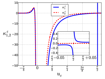
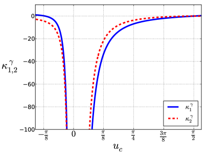
For the Gaussian distribution of frequencies $g(\omega)=\frac{1}{\sqrt{2\pi}}e^{-\frac{x^{2}}{2}}$ the constant $Q$ can be evaluated explicitly and it is equal to one. In the latter case calculations of (25) show (Fig. 9) that $\kappa^{\varepsilon,\gamma}_{1,2}(u_{c})$ are finite and non-zero everywhere except for mentioned above singular points $u_{c}=0$ and $u_{c}=\pi/2$, which correspond to the one-harmonic Kuramoto model where the transition has a continuous second-order type form.

Figure 9: Dependences of $\kappa^{\varepsilon,\gamma}_{1,2}$ on $u_{c}$.

5 Asymmetric coupling function

Figure 10: Dependences of the order parameters $R_{1,2}$ and their frequency $\Omega$ on coupling strength $\varepsilon$ at fixed values of $\beta_{1,2}$ and $\gamma=1.5$. In the panel (a) $\beta_{1,2}=\pi/8$, in the panel (b) $\beta_{1,2}=\pi/4$. Here no normalization on the linear stability thresholds is performed.

In this section we present several examples of application of our general theory for calculation of uniformly rotating synchronous states for the case of non zero phase shifts $\beta_{1,2}$ in the coupling function, see Eqs. (15,16). Here the number of control parameters ($\varepsilon,\gamma,\beta_{1},\beta_{2}$) is large, thus we do not perform a comprehensive analysis but just illustrate applicability of the method.

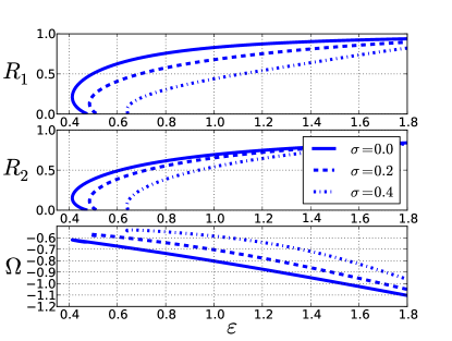
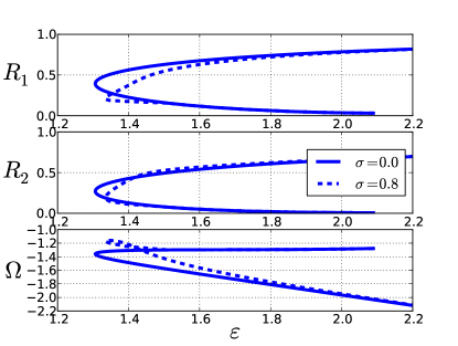
The main general feature at non-zero phase shifts $\beta_{1},\beta_{2}$ is a general appearance of a frequency shift $\Omega$, so that coherent solutions rotate with the frequency different from the mean frequency of the distribution $g(\omega)$. Figure 10 shows dependences of the order parameters $R_{1,2}$ and of frequency $\Omega$ on coupling constants $\varepsilon$ and $\gamma$, for fixed values of $\beta_{1,2}=\pi/8$ (Fig. 10(a)) and $\beta_{1,2}=\pi/4$ (Fig. 10(b)). These curves have been obtained from Eqs. (15,16) by adjusting free parameters $\mathbf{P}$ to achieve the given values of $\beta_{1},\beta_{2}$/

Another interesting example is motivated by work by Hansel et.al. [31] In this paper the authors consider an ensemble of identical (with equal natural frequencies) phase oscillators with a bi-harmonic coupling function. At $\pi/3<\beta_{1}<\pi/2$, $\beta_{2}=\pi$, $\varepsilon/\gamma=4$ the authors describe slow periodic oscillations of the order parameters and show that these variations arise due to a closed heteroclinic cycle in the phase space of the model. In order to model identical oscillators in our setup, one has to consider a delta-distribution of frequencies $g(\omega)=\delta(\omega)$. However, we have normalized the width of this distribution to one. Because normalization of frequencies is equivalent to normalization of time, in our approach the limit of identical oscillators corresponds to the limit $\varepsilon,\gamma\to\infty$ at a fixed width of the distribution $g(\omega)$. Thus, we applied our method for the parameters $\beta_{1,2}$ as in [31], for very large values of the coupling constants.

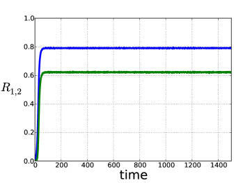
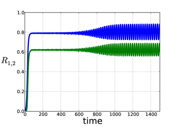
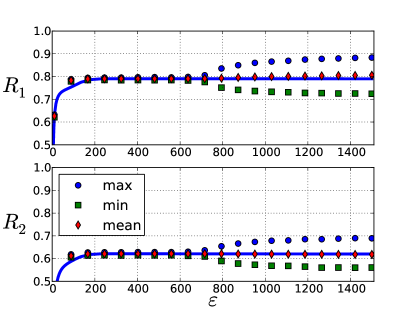
Figure 11(a) shows the solutions of equations (14-16) at $\beta_{1}=\pi/2.5$ $\beta_{2}=\pi$ and $\varepsilon/\gamma=4$, together with the results of direct numerical simulations of a large ensemble with $N=2\times 10^{4}$. At small values of coupling ($\varepsilon<650$), the stationary state obtained from our self-consistent approach is reproduced by direct numerical simulations of (1) (the time series is shown in Fig. 11(b)). At larger values of the coupling, this stationary solution loses stability via (presumably) a supercritical Andronov-Hopf bifurcation at which slow oscillatory variations of the order parameters appear (Fig. 11(c)). This example shows that while we always can find a uniformly rotating solution with constant order parameters, this solution can be unstable in some parameter range, where a more complex dynamics establishes.

(a)

(b) (c)

Figure 11: (a) Solutions of self-consistent equations (14-16) at $\beta_{1}=\pi/2.5$, $\beta_{2}=\pi$ and $\varepsilon/\gamma=4$ are shown. Markers (showing maximum, minimum and mean values of $R_{1,2}$ calculated from time series after some transient period) depict results of direct numerical simulation of equations (1) at the same parameters for $N=2\times 10^{4}$. The stationary state loses stability at a large coupling strength $\varepsilon\approx 650$, beyond which stable oscillations appear. (b,c) Time series of $R_{1,2}$ at different coupling strength are presented: in the panel (b) $\varepsilon=323$, in (c) $\varepsilon=1420$.

6 Conclusion

In this paper we have described nontrivial synchronous states that appear in the Kuramoto model with a bi-harmonic coupling function. Here we summarize essential novel features compared to the standard Kuramoto setup.

1. Due to a possibility to have two stable branches of phase-locked oscillators, one observes a multi-branch locking with a multiplicity of micro- states [28, 30]. On the macro-level, this multiplicity manifests itself as existence of a whole range of possible order parameters for given coupling constants. We have incorporated this multiplicity of multi-branch states into an analysis of self-consistent equations for the order parameters, and presented a general analytic solution.

2. Appearance of the synchronous states is not related to a standard bifurcation, as the asynchronous state does not change its neutral linear stability. We have found domains on the plane of basic coupling constants for the existence of such solutions, for different distributions of the locked phases between the branches (Fig. 3).

3. When a synchronous state is present, numerical experiments with finite ensembles show that the asynchronous state lives a finite time that scales like $T\sim N^{0.7}$, after which an abrupt transition to synchrony occurs. Similarly, we checked numerically stability of the states with single- and multi-branch entrainment through simulations of finite ensembles (Fig. 4).

4. At asymmetric distribution between the branches, the frequency of the order parameters deviates from the central frequency of the distribution, even if the latter and the coupling are symmetric.

Below we outline some open questions deserving further analysis. In the case of a general multi-harmonic coupling function $\Gamma$, one can expect existence of more than two stable brunches for oscillators at a particular frequency, with more possibilities for different redistributions of the oscillators phases. Another feature not addressed in this paper is related to a possibility of non-standard transitions to synchrony for particular distributions of the natural frequencies, similar to the analysis presented in Ref. [19] for the one-harmonic coupling. Detailed theoretical understanding of stability of the asynchronous states constructed via the self-consistency approach in this paper, is still missing. Finally, noise regularizes the multiplicity of the micro-states and turns neutral stability into an asymptotic one [40, 20]; these effects will be discussed in details elsewhere [22].

Appendix

Let us consider a system of $N$ pendulums (with mass $m$ and length $l$, described by angles $\theta_{j}$) suspended on a beam of mass $M$, which can move vertically (axis $y$) and horizontally (axis $x$) without rotation. These motions are controlled by two springs $k_{x}$ and $k_{y}$. This conservative system is described by the Lagrangean (cf. [41, 33])

$$L=\frac{M}{2}\left(\dot{x}^{2}+\dot{y}^{2}\right)+\frac{m}{2}\sum_{j}\left(\dot{x}^{2}+\dot{y}^{2}+l\dot{x}\dot{\theta_{j}}\cos\theta_{j}-l\dot{y}\dot{\theta_{j}}\sin\theta_{j}+l^{2}\dot{\theta_{j}}^{2}\right)+$$

$$+mgl\sum_{j}\cos\theta_{j}+gy\left(Nm+M\right)-\frac{k_{x}x^{2}}{2}-\frac{k_{y}y^{2}}{2}$$

The equations are two equations for the degrees of freedom of the beam (where we shift $y$ to the steady position $g(Nm+M)/ky$), and for each pendulum:

$$(M+Nm)\ddot{x}+k_{x}x=\sum_{j}-\frac{ml}{2}\ddot{\theta_{j}}\cos\theta_{j}+\sum_{j}\frac{ml}{2}\dot{\theta_{j}}^{2}\sin\theta_{j}$$

$$(M+Nm)\ddot{y}+k_{y}y=\sum_{j}\frac{ml}{2}\ddot{\theta_{j}}\sin\theta_{j}+\sum_{j}\frac{ml}{2}\dot{\theta_{j}}^{2}\cos\theta_{j}$$

$$ml^{2}\ddot{\theta_{j}}+mgl\sin\theta_{j}=\frac{ml}{2}\ddot{y}\sin\theta_{j}-\frac{ml}{2}\ddot{x}\cos\theta_{j}$$

In order to model self-sustained oscillations of the pendulum clocks, we add dissipation terms ($\sim\gamma_{x,y}$) to beam equations, and van-der-Pol-type self-exciation terms $\sim\sigma$, together with cubic saturation, to the pendula dynamics. In the case of small deviations $\theta_{1,2}$ (i.e. for $\sigma/rho\ll 1$) we have:

$$(M+Nm)\ddot{x}+\gamma_{x}\dot{x}+k_{x}x=\sum_{j}-\frac{ml}{2}\ddot{\theta_{j}}+\sum_{j}\frac{ml}{2}\dot{\theta_{j}}^{2}\theta_{j}$$ (26)

$$(M+Nm)\ddot{y}+\gamma_{y}\dot{y}+k_{y}y=\sum_{j}\frac{ml}{2}\ddot{\theta_{j}}\theta_{j}+\sum_{j}\frac{ml}{2}\dot{\theta_{j}}^{2}$$ (27)

$$\ddot{\theta_{j}}-(\sigma-\rho\theta_{j}^{2})\dot{\theta_{j}}+\omega^{2}\theta_{j}=\frac{1}{2l}\ddot{y}\theta_{j}-\frac{1}{2l}\ddot{x}$$ (28)

where $\omega^{2}=g/l$.

For small $\sigma\ll\omega$ we can apply the averaging (van der Pol) method. We will seek for a solution of the form:

$$\theta_{j}=A_{j}e^{i\omega t}+A^{*}_{j}e^{-i\omega t},\quad\dot{\theta}_{j}=i\omega(A_{j}e^{i\omega t}-A^{*}_{j}e^{-i\omega t})$$

where $A_{j}$ are slowly varying in time amplitudes.

Using this represntation, we can express the driving terms in the equations for the beam as follows:

$$\frac{ml}{2}\ddot{\theta_{j}}=-\frac{ml\omega^{2}}{2}\left(A_{j}e^{i\omega t}+A_{j}^{*}e^{-\omega t}\right)$$

$$\frac{ml}{2}\dot{\theta_{j}}^{2}\theta_{j}=-\frac{ml\omega^{2}}{2}\left(A_{j}^{3}e^{3\omega t}-|A|_{j}^{2}A_{j}e^{i\omega t}-A_{j}^{*}|A|_{j}^{2}e^{-i\omega t}+(A_{j}^{*})^{3}e^{-3\omega t}\right)$$

$$\frac{ml}{2}\ddot{\theta_{j}}\theta_{j}=-\frac{ml\omega^{2}}{2}\left(A_{j}^{2}e^{2i\omega t}+2|A|^{2}_{j}+(A^{*}_{j})^{2}e^{-2\omega t}\right)$$

$$\frac{ml}{2}\dot{\theta}_{j}^{2}=-\frac{ml\omega^{2}}{2}\left(A_{j}^{2}e^{2i\omega t}-2|A_{j}|^{2}+(A_{j}^{*})^{2}e^{-2i\omega t}\right)$$

Now the response of the beam to this driving can be expressed via solution of the linear equations, where the amplitudes $A$ are considered as constants:

$$x(t)=\sum_{j}\frac{ml\omega^{2}}{2}[H_{x}(\omega)A_{j}(1+|A|_{j}^{2})e^{i\omega t}+H^{*}_{x}(\omega)A^{*}_{j}(1+|A_{j}|^{2})e^{-i\omega t}-$$

$$-\left(H_{x}(3\omega)A_{j}^{3}e^{3\omega t}+H^{*}_{x}(3\omega)(A_{j}^{*})^{3}e^{-3\omega t}\right)]$$

$$y(t)=\sum_{j}-ml\omega^{2}\left[H_{y}(2\omega)A^{2}_{j}e^{2i\omega t}+H^{*}_{y}(2\omega)(A^{*}_{j})^{2}e^{-2i\omega t}\right]$$

and for the second derivatives we get

$$\ddot{x}(t)=\sum_{j}-\frac{ml\omega^{4}}{2}[H_{x}(\omega)A_{j}(1+|A|_{j}^{2})e^{i\omega t}+H^{*}_{x}(\omega)A^{*}_{j}(1+|A_{j}|^{2})e^{-i\omega t}-$$

$$-9\left(H_{x}(3\omega)A_{j}^{3}e^{3\omega t}+H^{*}_{x}(3\omega)(A_{j}^{*})^{3}e^{-3\omega t}\right)]$$

$$\ddot{y}(t)=\sum_{j}4ml\omega^{4}\left[H_{y}(2\omega)A^{2}_{j}e^{2i\omega t}+H^{*}_{y}(2\omega)(A^{*}_{j})^{2}e^{-2i\omega t}\right]$$

Here $H_{x,y}(\omega)$ are the response functions for the linear oscillators:

$$H_{x,y}(\omega)=\frac{1}{-\omega^{2}(M+Nm)+i\gamma_{x,y}\omega+k_{x,y}}$$

Equations for the complex amplitudes $A_{j}(t)$ follow from the rewriting Eq. (28) in terms of $A_{j}$ and averaging it over the fast time (basic period $2\pi/\omega$):

$$\dot{A}_{j}=\frac{1}{2}A_{j}\left(\sigma-\rho|A_{j}|^{2}\right)+\frac{1}{4i\omega l}\langle\ddot{y}\theta_{j}e^{-i\omega t}\rangle-\frac{1}{4i\omega l}\langle\ddot{x}e^{-i\omega t}\rangle$$

After averaging only the terms with $\ddot{y}\theta_{j}\sim e^{i\omega t}$ and $\ddot{x}\sim e^{i\omega t}$ survive:

$$\dot{A_{j}}=\frac{1}{2}A_{j}\left(\sigma-\rho|A_{j}|^{2}\right)+DA_{j}^{*}\sum_{k}A_{k}^{2}+S\sum_{k}A_{k}$$

where

$$D=-im\omega^{3}H_{y}(2\omega),\qquad S=-\frac{im\omega^{3}}{8}H_{x}(\omega)$$

[here we neglected terms containing higher orders in $A_{j}$, due to smallness of the amplitudes]. Terms $\sim D$ arise from the vertical motion of the beam $\ddot{y}$, while terms $\sim S$ are due to the horizontal motion $\ddot{x}$.

In the phase approximation we assume that the amplitudes $|A_{j}|$ are nearly constants $|A_{j}|=\sqrt{\sigma/\rho}$ and the interaction does not affect their dynamics. Therefore for phases $\phi_{j}$ ($A_{j}=|A_{j}|e^{i\phi_{j}}$) we have the following equations:

$$\dot{\phi_{j}}=\Omega+d\sum_{k}\sin(2(\phi_{k}-\phi_{j})+\beta)+s\sum_{k}\sin(\phi_{k}-\phi_{j}+\alpha)$$ (29)

where $d=\sigma\rho^{-1}|D|$, $s=|S|$, $\beta=arg(D)$ and $\alpha=arg(S)$. The freqeuncy is determined as $\Omega=Im\left(\sigma\rho^{-1}D+S\right)$. The obtained system is the Kuramoto model with bi-harmonic coupling.

References

• [1] K. Wiesenfeld, J. W. Swift, Averaged equations for Josephson junction series arrays, Phys. Rev. E 51 (2) (1995) 1020–1025.
• [2] K. Wiesenfeld, P. Colet, S. H. Strogatz, Synchronization transition in a disordered Josephson series array, Phys. Rev. Lett. 76 (3) (1996) 404–407.
• [3] K. Wiesenfeld, P. Colet, S. Strogatz, Frequency locking in Josephson arrays: Connection with the Kuramoto model, Physical Review E 57 (2) (1998) 1563–1569.
• [4] I. Kiss, Y. Zhai, J. Hudson, Emerging coherence in a population of chemical oscillators, Science 296 (2002) 1676–1678.
• [5] J. Grollier, V. Cros, A. Fert, Synchronization of spin-transfer oscillators driven by stimulated microwave currents, Phys. Rev. B 73 (2006) 060409(R).
• [6] B. Georges, J. Grollier, V. Cros, A. Fert, Impact of the electrical connection of spin transfer nano-oscillators on their synchronization: an analytical study, Applied Physics Letters 92 (23) (2008) 232504. doi:10.1063/1.2945636.
URL http://link.aip.org/link/?APL/92/232504/1
• [7] B. Eckhardt, E. Ott, S. H. Strogatz, D. M. Abrams, A. McRobie, Modeling walker synchronization on the Millennium Bridge, Phys. Rev. E 75 (2007) 021110.
• [8] Z. Néda, E. Ravasz, T. Vicsek, Y. Brechet, A. L. Barabási, Physics of the rhythmic applause, Phys. Rev. E 61 (2000) 6987–6992. doi:10.1103/PhysRevE.61.6987.
URL http://link.aps.org/doi/10.1103/PhysRevE.61.6987
• [9] D. Golomb, D. Hansel, G. Mato, Mechanisms of Synchrony of Neural Activity in Large Networks, in: F. Moss, S. Gielen (Eds.), Neuro-informatics and Neural Modeling, Vol. 4 of Handbook of Biological Physics, Elsevier, Amsterdam, 2001, pp. 887–968.
• [10] M. Breakspear, S. Heitmann, A. Daffertshofer, Generative models of cortical oscillations: neurobiological implications of the Kuramoto model, Frontiers in human neuroscience 4 (2010) 190.
• [11] D. Gonze, S. Bernard, C. Waltermann, A. Kramer, H. Herzel, Spontaneous synchronization of coupled circadian oscillators, Biophysical Journal 89 (1) (2005) 120 – 129. doi:http://dx.doi.org/10.1529/biophysj.104.058388.
URL http://www.sciencedirect.com/science/article/pii/S0006349505726643
• [12] G. Bordyugov, P. Westermark, A. Korencic, H. Herzel, Mathematical Modelling in Chronobiology, in: A. Kramer, M. Merrow (Eds.), Circadian Clocks, Springer, 2013.
• [13] Y. Kuramoto, Chemical Oscillations, Waves and Turbulence, Springer, Berlin, 1984.
• [14] A. Pikovsky, M. Rosenblum, J. Kurths, Synchronization. A Universal Concept in Nonlinear Sciences., Cambridge University Press, Cambridge, 2001.
• [15] Y. Kuramoto, Self-entrainment of a population of coupled nonlinear oscillators, in: H. Araki (Ed.), International Symposium on Mathematical Problems in Theoretical Physics, Springer Lecture Notes Phys., v. 39, New York, 1975, p. 420.
• [16] J. A. Acebrón, L. L. Bonilla, C. J. P. Vicente, F. Ritort, R. Spigler, The Kuramoto model: A simple paradigm for synchronization phenomena, Rev. Mod. Phys. 77 (1) (2005) 137–175.
• [17] E. Ott, T. M. Antonsen, Low dimensional behavior of large systems of globally coupled oscillators, CHAOS 18 (3) (2008) 037113.
• [18] E. Ott, T. M. Antonsen, Long time evolution of phase oscillator systems, CHAOS 19 (2) (2009) 023117.
• [19] O. E. Omel’chenko, M. Wolfrum, Nonuniversal transitions to synchrony in the sakaguchi-kuramoto model, Phys. Rev. Lett. 109 (2012) 164101.
• [20] M. Komarov, A. Pikovsky, Multiplicity of singular synchronous states in the Kuramoto model of coupled oscillators, Phys. Rev. Lett. 111 (2013) 204101. doi:10.1103/PhysRevLett.111.204101.
URL http://link.aps.org/doi/10.1103/PhysRevLett.111.204101
• [21] K. Li, S. Ma, H. Li, J. Yang, Transition to synchronization in a kuramoto model with the first- and second-order interaction terms, Phys. Rev. E 89 (2014) 032917.
• [22] V. Vlasov, M. Komarov, A. Pikovsky, unpublished (2014).
• [23] H. Sakaguchi, Y. Kuramoto, A soluble active rotator model showing phase transition via mutual entrainment, Prog. Theor. Phys. 76 (3) (1986) 576–581.
• [24] J. D. Crawford, Scaling and singularities in the entrainment of globally coupled oscillators, Phys. Rev. Lett. 74 (21) (1995) 4341–4344.
• [25] J. D. Crawford, K. T. R. Davies, Synchronization of globally coupled phase oscillators: Singularities and scaling for general couplings, Physica D 125 (1-2) (1999) 1–46.
• [26] H. Daido, Onset of cooperative entrainment in limit-cycle oscillators with uniform all-to-all interactions: Bifurcation of the order function, Physica D 91 (1996) 24–66.
• [27] H. Chiba, I. Nishikawa, Center manifold reduction for large populations of globally coupled phase oscillators, Chaos 21 (4) (2011) 043103. doi:10.1063/1.3647317.
URL http://link.aip.org/link/?CHA/21/043103/1
• [28] A. T. Winfree, The Geometry of Biological Time, Springer, Berlin, 1980.
• [29] H. Daido, Multi-branch entrainment and multi-peaked order-functions in a phase model of limit-cycle oscillators with uniform all-to-all coupling, J. Phys. A: Math. Gen. 28 (1995) L151–L157.
• [30] H. Daido, Multibranch entrainment and scaling in large populations of coupled oscillators, Phys. Rev. Lett. 77 (7) (1996) 1406–1409.
• [31] D. Hansel, G. Mato, C. Meunier, Clustering and slow switching in globally coupled phase oscillators, Phys. Rev. E 48 (1993) 3470–3477. doi:10.1103/PhysRevE.48.3470.
URL http://link.aps.org/doi/10.1103/PhysRevE.48.3470
• [32] P. S. Skardal, E. Ott, J. G. Restrepo, Cluster synchrony in systems of coupled phase oscillators with higher-order coupling, Phys. Rev. E 84 (2011) 036208. doi:10.1103/PhysRevE.84.036208.
URL http://link.aps.org/doi/10.1103/PhysRevE.84.036208
• [33] K. Czolczyński, P. Perlikowski, A. Stefański, T. Kapitaniak, Synchronization of the self-excited pendula suspended on the vertically displacing beam, Communications in Nonlinear Science and Numerical Simulation 18 (2) (2013) 386 – 400.
• [34] E. Goldobin, D. Koelle, R. Kleiner, R. G. Mints, Josephson junction with a magnetic-field tunable ground state, Phys. Rev. Lett. 107 (2011) 227001.
• [35] I. Z. Kiss, Y. Zhai, J. L. Hudson, Predicting mutual entrainment of oscillators with experiment-based phase models, Phys. Rev. Lett. 94 (2005) 248301.
• [36] I. Z. Kiss, Y. Zhai, J. L. Hudson, Characteristics of cluster formation in a population of globally coupled electrochemical oscillators: An experiment-based phase model approach, Prog. Theor. Phys. Suppl. 161 (2006) 99–106.
• [37] S. H. Strogatz, R. E. Mirollo, Stability of incoherence in a population of coupled oscillators, J. Stat. Phys. 63 (3/4) (1991) 613–635.
• [38] N. G. V. Kampen, On the theory of stationary waves in plasmas, Physica 21 (1955) 949–963.
• [39] H. Daido, Generic scaling at the onset of macroscopic mutual entrainment in limit-cycle oscillators with uniform all-to-all coupling, Phys. Rev. Lett. 73 (5) (1994) 760–763.
• [40] T. Aonishi, M. Okada, Multibranch entrainment and slow evolution among branches in coupled oscillators, Phys. Rev. Lett. 88 (2001) 024102. doi:10.1103/PhysRevLett.88.024102.
URL http://link.aps.org/doi/10.1103/PhysRevLett.88.024102
• [41] M. Kapitaniak, K. Czolczyński, P. Perlikowski, A. Stefański, T. Kapitaniak, Synchronization of clocks, Physics Reports 517 (1-2) (2012) 1–69.