The Pattern Method for Incorporating Tidal Uncertainty Into Probabilistic Tsunami Hazard Assessment (PTHA)

Abstract

In this paper we describe a general framework for incorporating tidal uncertainty into probabilistic tsunami hazard assessment and propose the Pattern Method and a simpler special case called the $\Delta t$ Method as effective approaches. The general framework also covers the method developed by Mofjeld et al (2007) that was used for the 2009 Seaside, Oregon probabilistic study by González et al (2009). We show the Pattern Method is superior to past approaches because it takes advantage of our ability to run the tsunami simulation at multiple tide stages and uses the time history of flow depth at strategic gauge locations to infer the temporal pattern of waves that is unique to each tsunami source. Combining these patterns with knowledge of the tide cycle at a particular location improves the ability to estimate the probability that a wave will arrive at a time when the tidal stage is sufficiently large that a quantity of interest such as the maximum flow depth exceeds a specified level.

1 Introduction

A numerical tsunami modeling code typically takes as input the seafloor deformation due to an event (such as an earthquake or submarine landslide) and then simulates the resulting tsunami generation and propagation. Often the desired output is a map of the maximum depth of flooding, maximum flow velocity, or some other quantity of interest over some region along the coast. We will use $\zeta(x,y)$ to denote some generic Quantity of Interest (QoI) that might be computed as a function of spatial location (typically maximizing some non-negative quantity over the entire duration of the tsunami event). We use the open source GeoClaw model (http://www.clawpack.org/geoclaw) described in detail by Berger et al (2010) and LeVeque et al (2011), but the methodology developed here could be used in conjunction with other tsunami modeling codes.

One use of such models is in performing Probabilistic Tsunami Hazard Assessment (PTHA), in which a probability distribution is specified over a space of possible seafloor deformations and the desired output is a probabilistic map of the QoI: At each point $(x,y)$ in the region of interest we wish to estimate the annual probability that $\zeta(x,y)$ will exceed some value $\hat{\zeta}$, typically for a specified set of exceedance values $\hat{\zeta}=\zeta_{1},~{}\zeta_{2},~{}\ldots,~{}\zeta_{I}$. A curve that shows the annual probability of exceedance $P[\zeta(x,y)>\hat{\zeta}]$ as a function of $\hat{\zeta}$ is called a hazard curve, and plotting contours derived from these hazard curves constructed at each point on a dense grid of $(x,y)$ locations gives the desired hazard map.

There are many uncertainties that must be taken into account in performing PTHA. The largest source of epistemic uncertainty is the paucity of knowledge of the proper probability distribution for seafloor deformations. PTHA associated with subduction zone megathrust events (e.g. Sumatra 2004, Maule 2010, Tohoku 2011) is typically done by first developing a finite set of “characteristic earthquakes” that are thought to be representative of possible events and assigning an annual probability of occurrence to each. If this correctly described the probability distribution, and if there were no other sources of uncertainty, then computing the QoI via a single tsunami simulation for each event would give a set of values that could be easily combined into the desired hazard curves.

There are many other sources of uncertainty that must also be considered in a full PTHA. In this paper we consider one important source of aleatoric uncertainty: the fact that for hypothetical tsunamis in the future we do not know whether the tsunami will reach the region of interest at high tide or low tide and the effect can be considerably different in some cases depending on the tide stage. We assume the region of interest is sufficiently small (e.g. a single harbor or city) that the tide can be described by a single function $\xi(t)$ that is measured in meters relative to Mean Sea Level (MSL) in this region. We also assume we know $\xi(t)$ for all $t$ spanning a sufficiently long time period (e.g. one year) that we can assume this time series properly describes the statistical properties of the tide. Tide gauge records are available at many locations that can be used, or $\xi(t)$ can be determined analytically from Fourier series with known coefficents for the tidal constituents, which have also been determined for many locations. With this assumption, there is no epistemic uncertainty in the tide and we have only the aleatoric uncertainty associated with the fact that the earthquake could happen at any time, which means that the time $t_{0}$ of the first arrival of a tsunami at the region of interest can be viewed as a random variable that is uniformly distributed over the time period for which we have the representative tidal record $\xi(t)$.

The tide function $\xi(t)$ represents the tide at the location of interest as a function of time, relative to Mean Sea Level (MSL) which is taken to be $\xi_{\scriptscriptstyle MSL}=0$. Certain site-specific values will be referred to below and we summarize these here, adapted from http://tidesandcurrents.noaa.gov/datum_options.html. Typically the tide function $\xi(t)$ exhibits two high tides each tidal day, one of which is often considerably higher than the other. The value $\xi_{\scriptscriptstyle MHW}$ (Mean High Water) denotes the average of all the high water heights observed over the National Tidal Datum Epoch, while $\xi_{\scriptscriptstyle MHHW}$ (Mean Higher High Water) denotes the average of the higher high water height of each tidal day. Similarly, $\xi_{\scriptscriptstyle MLW}$ and $\xi_{\scriptscriptstyle MLLW}$ denote Mean Low Water and Mean Lower Low Water, respectively. Finally $\xi_{\scriptscriptstyle LAT}$ and $\xi_{\scriptscriptstyle HAT}$ denote the lowest and highest predicted astronomical tide expected to occur at the site. (Observed tides may be higher or lower due to non-astronomical effects such as storm surge or other meterological effects, for example). Values for Crescent City are given in Section 5.1.

In this paper we focus entirely on the following question: Given that a particular tsunami-generating event $E$ occurs, what is the probability that $\zeta(x,y)$ exceeds some specified level $\hat{\zeta}$? We are not concerned with estimating the probability that $E$ occurs (or any sources of uncertainty other than the fact that $t_{0}$ is a random variable distributed uniformly as described above), and so we are really concerned with the conditional probability $P[\zeta>\hat{\zeta}\,|\,E]$, where the only randomness is in $t_{0}$. Note that if $P_{E}$ is the probability that event $E$ occurs, then the annual probability of exceeding $\hat{\zeta}$ due to this event is then given by the product $P_{E}P[\zeta>\hat{\zeta}\,|\,E]$ and it is these probabilities that are combined with those from other events to obtain the hazard curves. Henceforth we simplify notation by simply writing $P[\zeta>\hat{\zeta}]$ for the conditional probability and assume we are focusing on one possible event. Note that we also drop the explicit dependence on $(x,y)$ for brevity, but these conditional probabilities will vary in space and must be computed separately at each point of interest.

2 Background and context

The methods and theory presented in this paper were first developed in conjunction with a PTHA study (González et al, 2013) of Crescent City, California funded by BakerAECOM and motivated by FEMA’s desire to improve products of the FEMA Risk Mapping, Assessment, and Planning (Risk MAP) Program. At Crescent City, the difference in tide level between Mean Lower Low water (MLLW) and Mean Higher High water (MHHW) is about 2.1 meters. Coastal sites with such a significant tidal range experience tsunami/tide interactions that are an important factor in the degree of flooding. For example, Kowalik and Proshutinsky (2010) conducted a modeling study that focused on two sites, Anchorage and Anchor Point, in Cook Inlet, Alaska. They found tsunami/tide interactions to be very site-specific, with strong dependence on local bathymetry and coastal geometry, and concluded that the tide-induced change in water depth was the major factor in tsunami/tide interactions. Similarly, a study of the 1964 Prince William Sound tsunami (Zhang et al, 2011) compared simulations conducted with and without tide/tsunami interactions. They also found large site-specific differences and determined that tsunami/tide interactions can account for as much as 50% of the run-up and up to 100% of the inundation. Thus, probabilistic tsunami hazard assessment (PTHA) studies must account for the uncertainty in tidal stage during a tsunami event.

Houston and Garcia (1978) developed probabilistic tsunami inundation predictions that included tidal uncertainty for points along the US West Coast. The study was conducted for the Federal Insurance Agency, which needed such assessments to set federal flood insurance rates. They considered only far-field sources in the Alaska-Aleutian and Peru-Chile Subduction Zones, because local West Coast sources such as the CSZ (Cascadia Subduction Zone) and Southern California Bight landslides, http://www.usc.edu/dept/tsunamis/2005/pdf/GRL2004BorreroEtal.pdf, had not yet been discovered, and assigned probabilities to each source based on the work of Soloviev (2011). Maximum runup estimates were made at 105 coastal sites rather than from actual inundation computations on land. The tidal uncertainty methodology began with a modeled 2-hour tsunami time series that was extended by 24-hours by appending a sinusoidal wave with an amplitude that was 40% of the maximum modeled wave, to approximate the observed decay of West Coast tsunamis. This 24-hour tsunami time series was then added sequentially to 35,040 24-hour segments of a year-long record of the predicted tides, each segment being temporally displaced by 15 minutes. Determination of the maximum value in each 24-hour segment then yielded a year-long record of maximum combined tide and tsunami elevations, each associated with the probability assigned to the corresponding far-field source. Ordering the elevations and, starting with the largest elevations, summing elevations and probabilities to the desired levels of 0.01 and 0.002, produced the 100-year and 500-year elevations, respectively.

Mofjeld et al (2007) developed a tidal uncertainty methodology that, unlike that of (Houston and Garcia, 1978), does not use modeled tsunami time series. Instead, a family of synthetic tsunami series are constructed, each with a period in the tsunami mid-range of 20 minutes and an initial amplitude ranging from 0.5 to 9.0 m that decreases exponentially with the decay time of 2.0 days, as estimated by Van Dorn (1984) for Pacific-wide tsunamis. As in (Houston and Garcia, 1978), linear superposition of tsunami and tide is assumed and the time series are added sequentially to a year-long record of predicted tides at progressively later arrival times, in 15 minute increments. Direct computations are then made of the probability density function (PDF) of the maximum values of tsunami plus tide. The results are then approximated by a least squares fit Gaussian expression that is a function of known tidal constants for the area and the computed tsunami maximum amplitude; for this reason, we refer to this approach as the Gaussian method, or G Method. This expression provides a convenient means of estimating the tidal uncertainty, and was used by González et al (2009) in the PTHA study of Seaside, OR.

In this paper we present a unified framework that will be seen to include the G Method used by Mofjeld et al (2007) and González et al (2009). We also present the Pattern Method which falls within this unified framework but has the following improvements on that methodology: (a) The assumption of linear superposition of the tide and tsunami waves is replaced by a methodology that utilizes multiple runs at different tidal stages; thereby introducing nonlinearities in the inundation process that are not accounted for in previous methods. (b) Synthetic time series are replaced by the actual time series computed by the inundation model. (c) The Pattern Method takes account of temporal wave patterns that are unique to each tsunami source; for example, some sources produce only one large wave, others a sequence of equally dangerous waves that arrive over several hours. Combining these patterns with knowledge of the tide cycle at a particular location like Crescent City improves estimates of the probability that a wave will arrive at a time when the tidal stage is sufficiently large that inundation above a level of interest occurs. A special case of the Pattern Method that we call the $\Delta t$ Method is discussed first since it is easier to understand and implement, and may be sufficient for many tsunami studies.

In Section 3, we give an overview of our framework for calculating $P(\zeta>\hat{\zeta})$ assuming event $E$ has occurred. The $\Delta t$ Method, the Pattern Method, and the G Method are introduced and unified under this framework in Section 4. In Section 5, we use results from an example Crescent City PTHA study to compare these methods.

3 Overview of the framework

Recall that we consider one specific (hypothetical) tsunami event and one location $(x,y)$ and are attempting to compute the conditional probability that the QoI $\zeta(x,y)$ will exceed some value $\hat{\zeta}$, given that this event occurs. In practice we estimate these only for a set of discrete exceedance values $\hat{\zeta}=\zeta_{i}$ for $i=1,~{}2,~{}\ldots,I$, but the methodology can be described as a general approach to determining a complementary cumulative distribution function (CCDF) $\Psi(\hat{\zeta})$ such that

$$P[\zeta>\hat{\zeta}]\approx\Psi(\hat{\zeta}).$$ (1)

Recall that the random variable is the time $t_{0}$ at which the tsunami arrives, which is assumed to be uniformly distributed over a typical year of the tidal record, for example. All statements about probability are with respect to this underlying uniform distribution.

Once a specific tsunami event has been specified and a numerical method chosen to estimate the QoI, the only free parameter is the (static) tide stage $\hat{\xi}$ used to run the code. We assume it is possible to run the code for any choice of $\hat{\xi}$ and so in principle there is a function $\hat{Z}$ so that $\hat{\zeta}=\hat{Z}(\hat{\xi})$ is the value of the QoI that results from running the code with tide stage $\hat{\xi}$. In practice we cannot determine this function for all $\hat{\xi}$ in finite time, but we can approximate the function by various approaches and we refer to the approximation as $Z(\hat{\xi})$. In this paper we consider two possibilities:

• Run the code at a single tide level, for example taking a nearly worst-case value $\hat{\xi}=\xi_{\scriptscriptstyle MHHW}$, and then assume that for other values of $\hat{\xi}$ the value of $Z(\hat{\xi})$ varies in some specified manner. If the QoI is maximum depth of inundation, then assuming linear variation with slope 1 might be the natural choice. With this choice, any change in tide level is simply added to the inundation and

  $$Z(\hat{\xi})=\hat{Z}(\xi_{\scriptscriptstyle MHHW})+(\hat{\xi}-\xi_{\scriptscriptstyle MHHW}).$$ (2)

  This may be the only option when using a numerical model that does not allow adjusting the sea level parameter, and was used in the methodology developed in (Mofjeld et al, 2007), as discussed further in Section 4.3.

• Run the code at several values of $\hat{\xi}$ and use piecewise linear interpolation to approximate $Z(\hat{\xi})$ for intermediate values. If the set of $\hat{\xi}$ values used to approximate $Z$ does not span the full range of possibilities from $\xi_{\scriptscriptstyle LAT}$ to $\xi_{\scriptscriptstyle HAT}$, then it may still be necessary to use linear extrapolation beyond the largest $\hat{\xi}$ used, for example.

The second approach is preferable when possible, and we have found in our study of Crescent City that the relation between $\hat{\xi}$ and the maximum inundation can be very different from (2) in many onshore regions. Typical $Z$ functions for these two approaches are illustrated in the left plot in Figure 1.

Our methodology also requires the inverse function $Z^{-1}$, with the interpretation that $\hat{\xi}=Z^{-1}(\hat{\zeta})$ is the minimal tide level above which $\zeta$ exceeds $\hat{\zeta}$. If the function $Z(\hat{\xi})$ is monotonically increasing then $Z^{-1}$ is truly the inverse function. If $Z$ is non-monotone, then several tide levels $\hat{\xi}$ could result in the same value of $\zeta$. As a conservative choice we might want to choose the smallest tide level above which the QoI exceeds level $\hat{\zeta}$ (i.e. the infimum of the open set of points where $Z(\hat{\xi})>\hat{\zeta}$), and so we could define

$$Z^{-1}(\hat{\zeta})\equiv\inf(\hat{\xi}:Z(\hat{\xi})>\hat{\zeta})$$ (3)

to make this function well-defined. (For some quantities of interest such as the maximum fluid velocity we have found that $Z(\hat{\zeta})$ may be far from monotone and there are also other alternatives, discussed briefly at the end of this section).

In addition to the functions $Z$ and $Z^{-1}$, the second main component of our general methodology is another CCDF, $\Phi(\hat{\xi})$, that allows us to map a specific tide level $\hat{\xi}$ to the probability that the tide will be above this level when the tsunami occurs. There are many approaches to defining this function, depending on how one interprets the phrase “when the tsunami occurs”. To explain the basic idea we first consider the simplest approximation, which is to assume that the tsunami consists of a single destructive wave that inundates and retreats over a much faster time scale than the rise and fall of the tide. In this case, we could choose $\Phi$ to be the function

$$\Phi_{0}(\hat{\xi})=P[\xi(t_{0})>\hat{\xi}]$$ (4)

where $t_{0}$ is a random time, sampled for example from a year of tidal records at the location of interest with a uniform distribution. This function $\Phi_{0}$ is easily approximated from available tide gauge records at many locations, or could be computed from $\xi(t)$ specified analytically from the tidal constituents, which have also been determined for many locations.

It is also sometimes useful to discuss the probability density $\phi(\hat{\xi})=-\Phi^{\prime}(\hat{\xi})$. Note that for the CCDF $\Phi_{0}$ of (4), the corresponding density $\phi_{0}$ has the property that

$$\int_{\hat{\xi}_{1}}^{\hat{\xi}_{2}}\phi_{0}(\hat{\xi})\,d\hat{\xi}=P[\hat{\xi}_{1}<\xi(t_{0})<\hat{\xi}_{2}],$$

where again $t_{0}$ is the uniformly distributed random variable and $\xi(t)$ is the known tidal variation function for the region of interest.

We can now explain how $\Psi$ in (1) is determined by our approach. If we accept $\Phi_{0}(\hat{\xi})$ as giving the probability that the tide will be above level $\hat{\xi}$ when a very short duration tsunami arrives, and if the tide level must be above some value $Z^{-1}(\hat{\zeta})$ in order for the QoI to exceed $\hat{\zeta}$, then clearly the probability of exceedance is $\Phi_{0}\left(Z^{-1}(\hat{\zeta})\right)$. This gives the definition of $\Psi(\hat{\zeta})$ we desire for (1). This is the key idea of our methodology. Several variants will be discussed in more detail based on our desire to improve on the choice $\Phi_{0}$.

Typically a tsunami does not consist of a single wave over a very short time duration, but rather a series of waves arriving over the course of several hours, during which the tide varies. In this case accurate modeling of the QoI might require a numerical model that also models the rise and fall of the tide and the resulting tidal currents and how they interact with the tsunami. Some work has been done in this direction, see (Androsov et al, 2011) and (Kowalik et al, 2006), but tsunami models currently in use for forcasting or hazard assessment work do not have this capability, even for modeling a specific event when the arrival time $t_{0}$ is known. Performing a probabilistic study where $t_{0}$ is random would be even more difficult since the model would have to be run with many different choices of $t_{0}$ to explore the full range of possibilities. Instead we focus on ways to improve the analysis in the practical case where the model can be run at different static tide levels $\hat{\xi}$ but not with dynamically varying tides.

We can still improve on the choice $\Phi_{0}$ in a number of ways, several of which are explored in this paper. If we know that destructive waves arrive over a time period of length $\Delta t$ then it is natural to consider the probability that the maximum value of $\xi(t)$ is above some specified level $\hat{\xi}$ over a random time interval $t_{0}\leq t\leq t_{0}+\Delta t$, which suggests the CCDF

$$\Phi_{\Delta t}(\hat{\xi})=P\left[\max_{t_{0}\leq t\leq t_{0}+\Delta t}\xi(t)>\hat{\xi}\right].$$ (5)

Again $t_{0}$ is the random variable, uniformly distributed over 1 year, say. Note that for $\Delta t=0$ this reduces to $\Phi_{0}$ defined in (4).

Several $\Phi_{\Delta t}$ curves are illustrated in Figure 1. The lowermost curve is $\Phi_{0}$ and as we increase the length of the time interval, the probability that $\xi(t)$ will be above a fixed $\hat{\xi}$ value over a random interval of this length will increase. The limiting curve as $\Delta t\rightarrow\infty$ is the discontinuous piecewise constant function

$$\Phi_{\infty}(\hat{\xi})=\left\{\begin{array}[]{ll}1&\mbox{if}~{}~{}\hat{\xi}<\xi_{\scriptscriptstyle HAT},\\ 0&\mbox{if}~{}~{}\hat{\xi}\geq\xi_{\scriptscriptstyle HAT}.\end{array}\right.$$ (6)

This results from the fact that over a sufficiently long time interval we are almost surely going to observe $\xi(t)$ above any value, up to the highest possible value that can be observed.

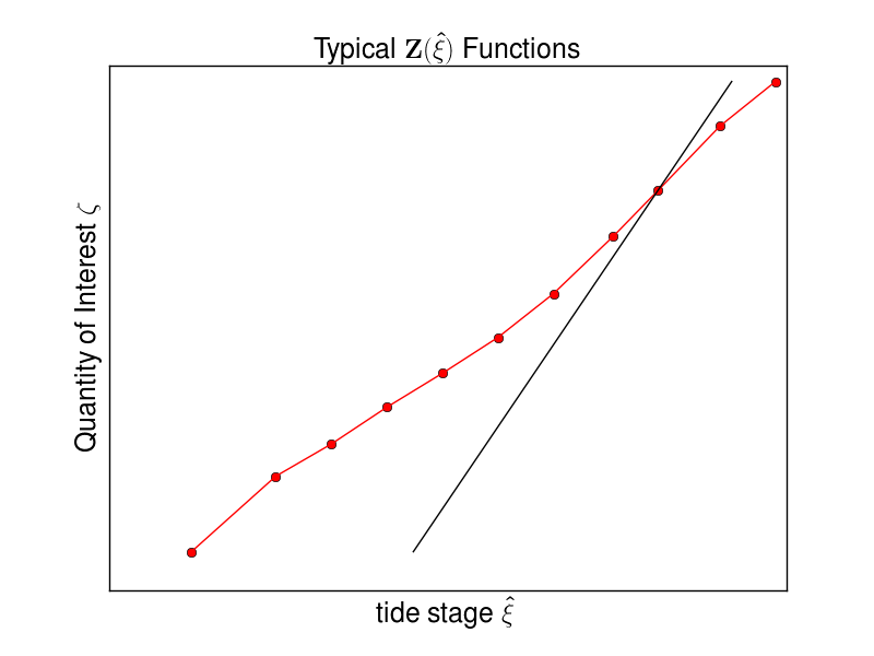
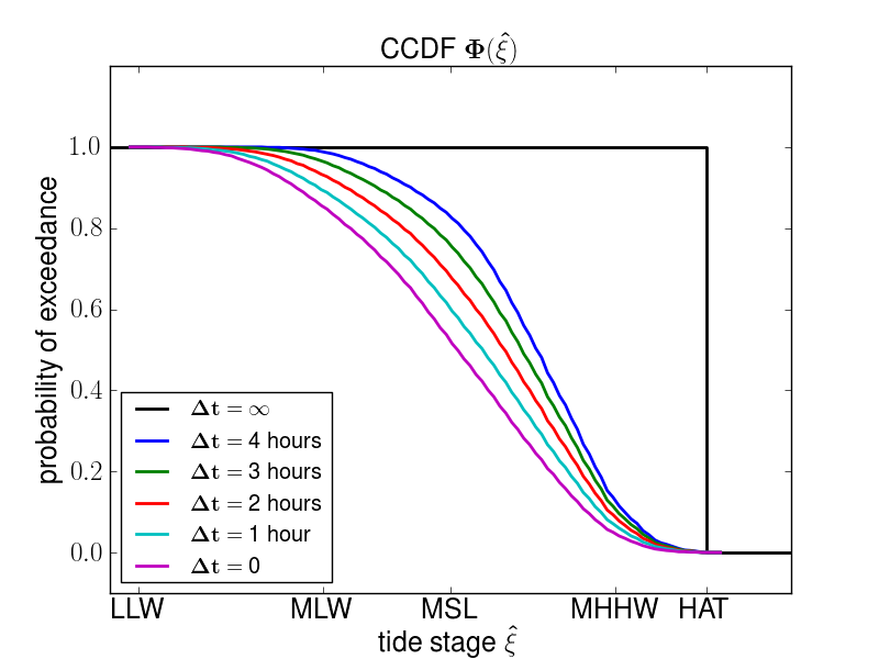
Figure 1: Left: Two possible functions $Z(\hat{\xi})$, a piecewise linear approximation (red) and a linear approximation based on a single run (black), Right: $\Phi_{\Delta t}(\hat{\xi})$

Choosing one of these $\Phi_{\Delta t}$ for $\Phi$ gives the $\Delta t$ Method described further in Section 4.1. These CCDF’s are also easily computed from tide gauge data or tidal constituents and for many tsunami events this may be a reasonable approach, estimating $\Delta t$ by examining the wave pattern observed in simulations.

For some events, however, there may be many destructive waves that arrive over the course of many hours or even several days, but interspersed by periods of no waves or outflow. In this case taking $\Delta t$ sufficiently large to capture all the waves might overestimate the probability that waves will arrive when the tide is high. So rather than looking at a single time interval of length $\Delta t$ starting at a random time $t_{0}$, it may be more accurate to specify a pattern of disjoint time intervals during which the large waves arrive, and then slide this pattern over the full tidal record to determine the probability that $\max_{t}\xi(t)$ will be above $\hat{\xi}$ (for $t$ ranging over this disjoint collection of time intervals, starting at some random time $t_{0}$). This approach can be made more general by also incorporating information about the relative magnitude of waves in the different intervals. This Pattern Method is discussed in more detail in Section 4.2.

Yet another approach to choosing $\Phi(\hat{\xi})$ would be to observe that most of the curves in Figure 1 resemble plots of the complementary error function (the CCDF corresponding to a Gaussian PDF) and choose

$$\Phi(\hat{\xi})=\frac{1}{2}\left(1-\text{erf}\left((\hat{\xi}-\xi_{0})/\sqrt{2}\sigma\right)\right),$$ (7)

for some choice of the mean $\xi_{0}$ and standard deviation $\sigma$. In Section 4.3 we show that the method proposed in (Mofjeld et al, 2007) can be reinterpreted in the framework of our methodology by making this choice for $\Phi$, even though the philosophy and derivation in that paper appear to be very different. In (Mofjeld et al, 2007), the parameters $\xi_{0}$ and $\sigma$ vary not only with the tsunami event being considered, but also with the specific point $(x,y)$ in the region of interest. In the $\Delta t$ Method or the Pattern Methods we recommend, the $\Phi$ might be chosen differently for different tsunami events (adjusting $\Delta t$ or the pattern), but the same $\Phi(\hat{\xi})$ is used for all $(x,y)$.

We now summarize the description of our general methodology. The key ingredients are the functions $Z$ (and hence the inverse $Z^{-1}$) and $\Phi$. Once these have been chosen, we estimate the probability that the QoI will exceed some level $\hat{\zeta}$ by

$$P[\zeta>\hat{\zeta}]\approx\Psi(\hat{\zeta})\equiv\Phi\left(Z^{-1}(\hat{\zeta})\right).$$ (8)

In practice this is applied for specific values of $\hat{\zeta}$, namely the exceedance values $\zeta_{i}$ of interest, in order to compute $\Psi(\zeta_{i})=\Phi(\hat{\xi}_{i})$ where $\hat{\xi}_{i}=Z^{-1}(\zeta_{i})$. In words, this means that for each exceedance level $\zeta_{i}$ we estimate the static tide level $\hat{\xi}_{i}$ above which $\zeta>\zeta_{i}$ in a tsunami simulation, and then we evaluate $\Phi(\hat{\xi}_{i})$ to determine the probability that the tide will be sufficiently high when the tsunami “arrives” (in the sense as encapsulated in the choice of $\Phi$).

This is further illustrated graphically in Figure 2. The top figure shows the function $Z(\hat{\xi})$. For a typical $\zeta_{i}$ on the vertical axis we invert $Z$ to find $\hat{\xi}_{i}$ on the horizontal axis. Then the bottom figure shows how this same value $\hat{\xi}_{i}$ is used to determine the desired probability by use of the function $\Phi$.

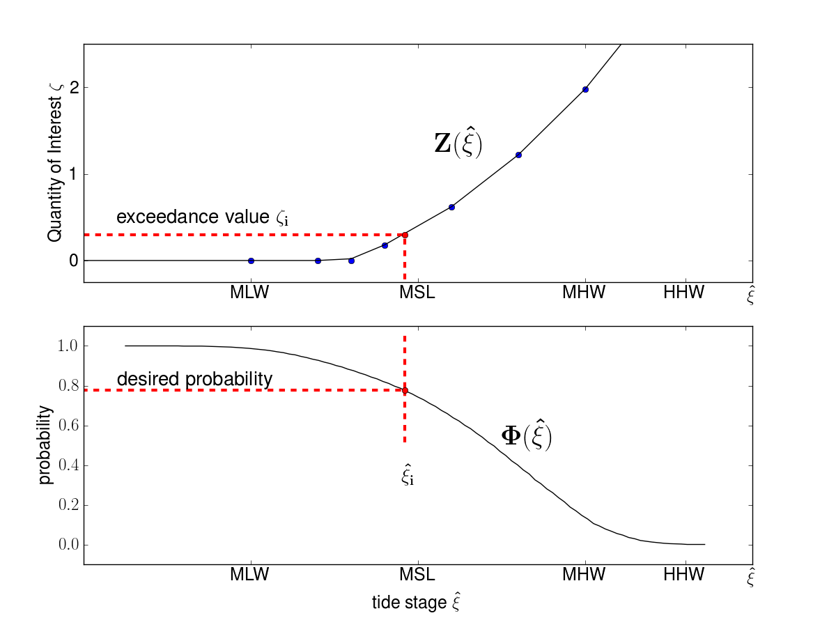
Figure 2: Determining $\Psi(\zeta_{i})$ by computing $\hat{\xi}_{i}=Z^{-1}(\zeta_{i}))$ and evaluating $\Phi(\hat{\xi}_{i})$.

Finally, we note that if $Z(\hat{\xi})$ is not a monotone function, then rather than using a single value $Z^{-1}(\hat{\zeta})$ defined by (3), we could instead determine the intervals $(\hat{\xi}_{j},\hat{\xi}_{j+1})$ over which $Z(\hat{\xi})>\hat{\zeta}$ and sum $\Phi(\hat{\xi}_{j})-\Phi(\hat{\xi}_{j+1})$ over all such intervals to define $\Psi(\hat{\zeta})$.

4 Methods based on the framework

We need to estimate $P[\zeta>\hat{\zeta}]$ in equation (8), the probability that the QoI $\zeta$ exceeds $\hat{\zeta}$ whenever a given tsunami event occurs. We select a method for doing this by choosing a function $Z$ and a function $\Phi$, such as one of those depicted in Figure 1. The choices of these functions are given in Section 4.1 for the $\Delta t$ Method, in Section 4.2 for the Pattern Method and in Section 4.3 for the G Method. These methods are then compared in Section 5 using tsunamis from the PTHA study in (González et al, 2013).

4.1 The $\Delta t$ Method

This method has been described briefly in Section 3. The function $Z(\hat{\xi})$ is chosen using the second approach outlined in Section 3. We typically use at least three values of $\hat{\xi}$ including $\xi_{\scriptscriptstyle MLLW}$, $\xi_{\scriptscriptstyle MSL}$, and $\xi_{\scriptscriptstyle MHHW}$ as sealevel parameters for GeoClaw simulations of the shallow water equations. The resulting $\hat{Z}$ values are used to make the piecewise linear $Z$ function shown in red in Figure 1.

Once $\Delta t$ has been selected for a particular tsunami, the function $\Phi(\hat{\xi})$ is given in equation (5) and its graph can be found in Figure 1. Discrete values of $\Phi(\hat{\xi})$ are gotten by first placing valid values of $\hat{\xi}$ in bins and then using a $\Delta t$-window of time and sliding it one minute at a time across a year’s worth of tide gauge data at the tsunami destination site of interest. Each time the $\Delta t$-slider window stops, we find the maximum tide level within the window. We increment a counter in the first bin whose right edge exceeds or equals this maximum (to create a histogram) and also in all lower bins (to create a cumulative histogram). Dividing by the number of times the $\Delta t$-slider window stops gives the probability mass function and $\Phi(\hat{\xi})$, respectively. The PDF $\phi(\hat{\xi})$ results by dividing the probability mass function by the bin size. The $\Phi$ values for each bin’s left edge are stored in a table and interpolated as needed.

Different tsunamis will require different choices of $\Delta t$. We place computational gauges at various locations where we collect time series output to determine the width and relative occurrence times of potentially damaging waves. The width of the responsible wave of biggest amplitude certainly gives a minimum value for the contiguous $\Delta t$ interval, and we increase $\Delta t$ if there are nearby waves of nearly equal amplitude, so the tsunami is effectively modelled as one square wave of width $\Delta t$.

In Section 5, we see the $\Delta t$ Method works remarkably well compared to the Pattern Method for appropriately chosen $\Delta t$, and there we give recommended values for particular tsunamis in the Crescent City study.

4.2 The Pattern Method

$Z(\hat{\xi})$ is chosen the same as for the $\Delta t$ Method, see Section 4.1. When the tsunami consists of only one wave, we will see that the Pattern Method is simply the $\Delta t$ Method where $\Delta t$ is the time duration of the wave.

The Pattern Method uses the relative heights of the waves seen at a computational gauge located in the water, their widths, and the relative times they occurred, to create the $\Phi(\hat{\xi})$ associated with this particular wave pattern. This is extra work, but the difference is that a fixed $\Delta t$ will not have to be chosen. Instead, the entire pattern will be taken into account to calculate $\Phi(\hat{\xi})$.

Suppose the tsunami has $K$ waves. We model wave $W_{k}$ with a square wave and record the difference of its height from that of the highest wave as $D_{k}$. That is, $D_{k}=H-H_{k}$ where $H_{k}$ is the height of wave $W_{k}$, and $H=\max_{k}H_{k}$. We record the starting and terminating times of $W_{k}$ as the interval $I_{k}=[S_{k},T_{k}]$. These times are relative to the start of $W_{1}$, so we set $S_{1}=0$; they are recorded in minutes since our tide record has minute data. The pattern’s duration is then $T_{K}$ minutes.

As an example, in Figure 3, we show the GeoClaw tsunami for an Alaskan Aleutian event (AASZe02) in red and the pattern in black. The first wave arrived at Crescent City 4 hours and 23 minutes after the earthquake and nothing significant was seen there after 11 hours. The pattern is well represented by the 7 waves shown. We are overestimating the probability a bit by using square waves, but we don’t have to account for tides between these waves. Table 1 shows the values that describe the pattern. We note that the first wave began at 263 minutes after the earthquake and the amplitude of the largest wave $W_{7}$ was about 1.5 meters. The black horizontal line starts at 0.2 meters since the GeoClaw run was done at $\xi_{\scriptscriptstyle MHHW}$ which is 0.2 meters above $\xi_{\scriptscriptstyle MHW}$, the zero level for the plot in Figure 3.

Figure 3: Pattern for AASZe02

Table 1: Pattern Values Wave $I_{k}=[S_{k},T_{k}]$ $D_{k}$ (meters) $W_{k}$ Wave Interval Difference to (min since $S_{1}$) Tallest Wave $W_{1}$ [000, 042] 0.561 $W_{2}$ [084, 124] 0.498 $W_{3}$ [160, 202] 0.517 $W_{4}$ [243, 275] 0.782 $W_{5}$ [309, 325] 0.876 $W_{6}$ [342, 349] 1.450 $W_{7}$ [372, 396] 0.000

As in the $\Delta t$ Method, we put the valid values of $\hat{\xi}$ into bins. But now we take our pattern-slider window that has length $T_{K}$ and slide it one minute at a time across a year’s worth of the tidal record. Each time the window stops we calculate $\max_{1\leq k\leq K}(\,\max_{t\in I_{k}}\xi(t+t_{0})-D_{k}\,)$ corresponding to a different tsunami start time $t_{0}$. Then we increment a counter in the first bin whose right edge exceeds or equals this value (and in all lower bins) to create a histogram (cumulative histogram). These histograms are used as before to determine $\Phi$ and $\phi$ values. Thus, the Pattern Method $\Phi$ function is

$$\Phi_{\rm Pattern}(\hat{\xi})=P[\max_{1\leq k\leq K}(\,\max_{t\in I_{k}}\xi(t+t_{0})-D_{k}\,)>\hat{\xi}].$$ (9)

Note, that if the pattern consists of only one wave, then $D_{1}=0$ and the Pattern Method is just the $\Delta t$ Method with $\Delta t$ being the length of $I_{1}$. The Pattern Method has advantages over the $\Delta t$ Method. Only one synthetic gauge needs to be examined. A wave with amplitude less than the maximum one could also cause exceedance of $\hat{\zeta}$ if it occurred at a time when the tide level was sufficiently high. Tsunamis with longer duration are more accurately represented since the tide record during each interval $I_{k}$ and not between needs to be examined. This gives an automatic procedure that avoids the difficulty in choosing an appropriate $\Delta t$. A possible limitation is that the Pattern-Method requires the simulation code to have GeoClaw’s capability of a computational gauge.

4.3 The G Method

We describe how this method fits our framework in Section 3. Only one GeoClaw simulation at $\xi_{\scriptscriptstyle MHHW}$ is done to get $\hat{Z}(\xi_{\scriptscriptstyle MHHW})$. The function $Z(\hat{\xi})$ for location $(x,y)$ within the destination area of interest is then given in equation (2).

A proxy tsunami is assumed for each $(x,y)$, defined as having a duration of 5 days (or $T_{G}=7200$ minutes) with e-folding time of 2 days and period of 20 minutes with maximum amplitude $A_{G}=A_{G}(x,y)$. This assumed tsunami has maximum height $H$ which can be measured to any fixed reference level for our purposes and occurs with the first wave having amplitude $A_{G}$. Its height at time $t$ after the first wave begins is $H(t)$, and following previous notation, the distance to the maximum is $D(t)=H-H(t)$. Then $\Phi_{G}(\hat{\xi})$ is

$$\Phi_{G}(\hat{\xi})=P\,[\,\max_{t_{0}\leq t\leq t_{0}+T_{G}}(\xi(t)-D(t))\,]>\hat{\xi},$$ (10)

and can be further approximated by equation (7) with mean $\xi_{0}$ and standard deviation $\sigma$. Using $\hat{\zeta}=Z(\hat{\xi})$ and (2), we get $\hat{\xi}=\hat{\zeta}-\hat{Z}(\xi_{\scriptscriptstyle MHHW})+\xi_{\scriptscriptstyle MHHW}$ and (7) becomes

$$P[\zeta>\hat{\zeta}]\approx\frac{1}{2}\left(1-\rm{erf}\left((\hat{\zeta}-\zeta_{0})/\sqrt{2}\sigma\right)\right)$$ (11)

where the mean $\zeta_{0}$ of $\zeta$ is given by

$$\zeta_{0}=\hat{Z}(\xi_{\scriptscriptstyle MHHW})-\xi_{\scriptscriptstyle MHHW}+\xi_{0}.$$ (12)

This makes sense. As the value $\xi_{0}$ approaches $\xi_{\scriptscriptstyle MHHW}$, the mean of $\zeta$ should be $\hat{Z}(\xi_{\scriptscriptstyle MHHW})$. Also, $\zeta$’s value is $\hat{Z}(\xi_{\scriptscriptstyle MHHW})-\xi_{\scriptscriptstyle MHHW}$ when $\hat{\xi}=0$, or $\xi_{\scriptscriptstyle MSL}$. As $\xi_{0}$ approaches 0, $\zeta_{0}$ should approach this value.

We can now make the final connection to the formula for $P[\zeta>\hat{\zeta}]$ given in (Mofjeld et al, 2007). There, $\xi_{0}$ and $\sigma$ are functions of location $(x,y)$ and are given by $\xi_{0}=C\xi_{\scriptscriptstyle MHHW}e^{-\alpha{(A_{G}/\sigma_{0})}^{\beta}}$, and $\sigma=\sigma_{0}(1-C^{\prime}e^{-\alpha^{\prime}{(A_{G}/\sigma_{0})}^{\beta^{\prime}}})$. When $\zeta+\xi_{ref}$ is the flow depth above $\xi_{\scriptscriptstyle MSL}$, and $S$ is the amount of subsidence or uplift (positive with subsidence so that $\xi_{\scriptscriptstyle MHHW}-S$ is the subsided background water of the simulation), it makes sense to express $A_{G}$ as

$$A_{G}=\hat{Z}(\xi_{\scriptscriptstyle MHHW})+\xi_{ref}-(\xi_{\scriptscriptstyle MHHW}-S).$$ (13)

Substituting into (12) gives

$$\zeta_{0}=A_{G}-\xi_{ref}-S+C\xi_{\scriptscriptstyle MHHW}e^{-\alpha{(A_{G}/\sigma_{0})}^{\beta}}.$$ (14)

Using $\xi_{ref}=\xi_{\scriptscriptstyle MLLW}$ and $S=0$ gives the method in (Mofjeld et al, 2007), where the parameters are also given for a variety of tsunami destinations. Those for Crescent City include $\sigma_{0}=0.638$, the standard deviation for the tides there, and the regression parameters $\alpha^{\prime}$ = 0.056, $\beta^{\prime}$ = 1.119, $C^{\prime}$=0.707, $\alpha$=0.17, $\beta$=0.858, and $C$=1.044.

The G Method has two major limitations. First, only one GeoClaw simulation with tide level $\hat{\xi}=\xi_{\scriptscriptstyle MHHW}$ is used. This is appropriate whenever $Z(\hat{\xi})$ is indeed a linear function of slope 1, since then $A_{G}$ will be uniquely defined from only one simulation. The $Z(\hat{\xi})$ functions created with multiple simulations show this is not true, especially at onshore locations, see Figure 5.

The second limitation is the use of the same 5-day proxy tsunami (where the amplitude alone varies at each $(x,y)$) as the pattern for modelling each tsunami in a PTHA study, especially when the major question being studied is the flow depth at land points. As seen in Table 2, the duration of all the tsunamis studied that could impact the maximum inundation at a land point is much less than 5 days, and we observe these tsunamis have patterns that are very different. A local tsunami from the Cascadia Subduction Zone will typically have only one or two waves occuring over a short time frame that are responsible for the maximum; whereas, far field events can have damaging waves occuring over a longer time frame whose amplitudes can increase during significant tidal variations.

5 An example PTHA study and method comparisons

5.1 The Crescent City PTHA study

Phase I of the PTHA study of Crescent City, California reported in (González et al, 2013) focused on flow depths. Output products such as 100- and 500-year hazard maps, hazard curves at specific locations, and probability contours for exceeding a specific $\hat{\zeta}$ level can be found in the report. All these products used the Pattern Method. Here we demonstrate why this is the preferred method for including tidal uncertainty.

GeoClaw simulations of the shallow water equations were conducted at multiple static tide levels for each tsunami in the study to find the QoI at each fixed grid location. For this study, the QoI was the maximum flow depth above topography/bathymetry (onshore points) and the maximum flow depth plus the original bathymetry (offshore points) measured in meters and was denoted $\zeta$. For offshore points the bathymetry is negative, and represents the negative of the distance between the underwater topography and $\xi_{\scriptscriptstyle MHW}$. The QoI for offshore points is then the amount of flow depth above $\xi_{\scriptscriptstyle MHW}$ plus the amount of subsidence (original minus final bathymetry). The QoI for onshore points is the flow depth measured above the final topography. With this definition, the QoI is continuous at the shoreline which corresponds to $\xi_{\scriptscriptstyle MHW}$.

The GeoClaw simulations made use of computational gauges placed at strategic locations where the time series of the QoI were monitored. One such gauge, called Gauge 101, was placed in the Crescent City harbor and was where some of our results are reported. In particular, this gauge is where we recorded each tsunami’s pattern for the Pattern Method.

A few important tidal constants at Crescent City Gauge No. 9419750, see http://tidesandcurrents.noaa.gov/waterlevels.html?id=9419750, that were used as sealevel parameters for GeoClaw simulations are Mean Lower Low Water ($\xi_{\scriptscriptstyle MLLW}=-1.13$), Mean Low Water ($\xi_{\scriptscriptstyle MLW}=-0.75$), Mean Sea Level ($\xi_{\scriptscriptstyle MSL}=0.0$), Mean High Water ($\xi_{\scriptscriptstyle MHW}=0.77$), and Mean Higher High Water ($\xi_{\scriptscriptstyle MHHW}=0.97$). The lowest and highest water seen at the gauge in a year’s data from July 2011 to July 2012 are $\xi_{Lowest}=-1.83$ and $\xi_{Highest}=1.50$ in meters, referenced to $\xi_{\scriptscriptstyle MSL}$ respectively. Figure 4 shows the PDF $\phi_{0}(\hat{\xi})$ and the CCDF $\Phi_{0}(\hat{\xi})$ for this yearly data. $\Phi_{0}(\hat{\xi})$ is that of the $\Delta t=0$ Method.

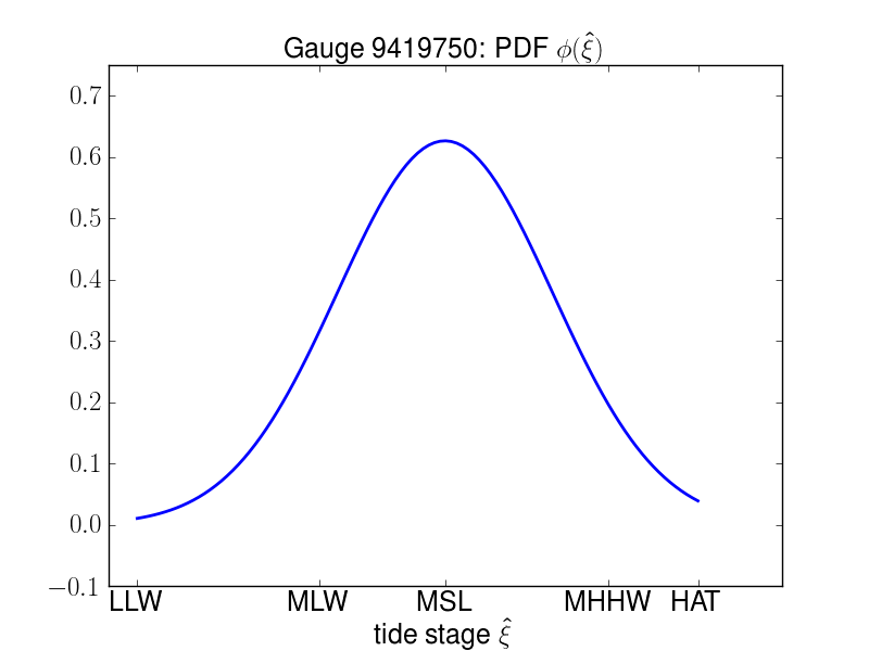
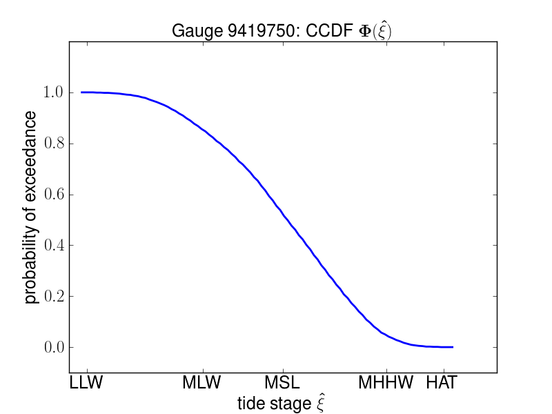
Figure 4: Crescent City Tides: Left: $\phi_{0}(\hat{\xi})$ ($\xi_{0}=0.0$, $\sigma_{0}$ = 0.638), Right: $\Phi_{0}(\hat{\xi})$

Column 1 of Table 2 gives representative tsunamis used in this PTHA study. The acronyms CSZ, AASZ, KmSZ, KrSZ, and SchSZ stand for the Cascadia, Alaskan Aleutian, Kamchatka, Kuril, and South Chile Subduction Zones, respectively, and TOH refers to Tohoku. We also denote tsunami events in the form AASZe03; for example, event number 3 on the Alaska Aleutian Subduction Zone. Some events, e.g., a CSZ Mw 9.1 event, have multiple realizations. CSZBe01r01-CSZBe01r15 refers to the CSZ Bandon sources modeled as 15 realizations of different slip distributions for a single event used in a PTHA study of Bandon, Oregon (Witter et al, 2011). More details about these earthquake source models can be found in (González et al, 2013).

The recommended value of $\Delta t$ for all tsunamis in Table 2 and in (González et al, 2013) can be given. We recommend $\Delta t=1$ for the Kamchatka event KmSZe01 and $\Delta t=3$ for KmSZe02. For the three Kuril events, we recommend $\Delta t=2$ for KrSZe01, $\Delta t=3$ for KrSZe02, and $\Delta t=4$ for KrSZe03. For the Alaska events, we recommend $\Delta t=1$ with the exception of $\Delta t=2$ for AASZe02. The value $\Delta t=1$ should be used for the Chilean event SChSZ01, the Tohoku event TOHe01, and the Cascadia Bandon CSZBe01r13 and CSZBe01r14 tsunamis. The value $\Delta t=0$ should be used for the remaining Cascadia Bandon tsunamis, CSZBe01r01-CSZBe01r12 and CSZBe01r15.

For the $\Delta t$ and Pattern Methods most of these tsunami events were simulated by running GeoClaw at $\xi_{\scriptscriptstyle MLLW}$, $\xi_{\scriptscriptstyle MSL}$, and $\xi_{\scriptscriptstyle MHHW}$, respectively. For more intense analysis, the AASZe03 event (similar to the 1964 Alaska tsunami) was run using 11 tide levels. These levels referenced to $\xi_{\scriptscriptstyle MSL}$ were -1.13, -0.75, -0.50, -0.25, 0.00, 0.25, 0.50, 0.77, 0.97, 1.25, and 1.5 meters. For the G Method, only the GeoClaw $\xi_{\scriptscriptstyle MHHW}$ results were required.

Figure 5 gives the $Z(\hat{\xi})$ functions for four different locations for the AASZe03 tsunami. The black line on the plots is the $Z(\hat{\xi})$ used with the G Method and is the slope 1 line through the point corresponding to $\hat{\xi}=\xi_{\scriptscriptstyle MHHW}=0.97$. The red line is the $Z(\hat{\xi})$ used by the $\Delta t$ and Pattern Methods. The longitude, latitude, and bathymetry of the location is given on the graphs. The top row shows the $Z(\hat{\xi})$ function for two offshore locations is similar for all three methods. The second row shows the $Z(\hat{\xi})$ function for the $\Delta t$ and Pattern Methods for two onshore locations is far from the slope 1 line used by the G Method.

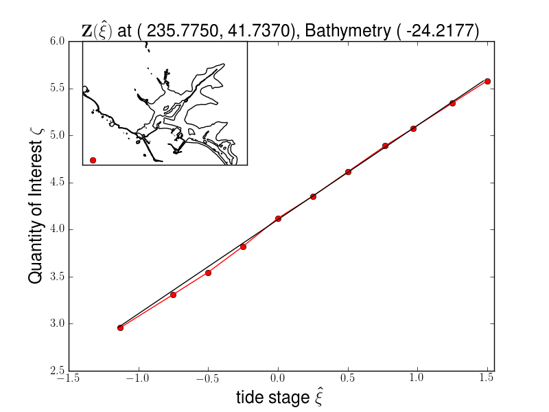
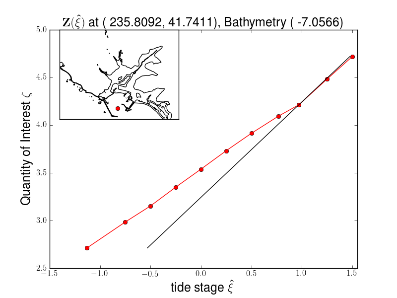
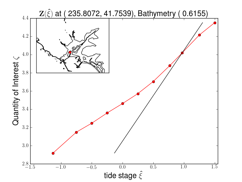
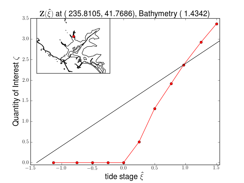
Figure 5: $Z(\hat{\xi})$ functions for flow depth at land locations (bottom row) and flow depth plus bathymetry at offshore locations (top row). Location longitude, latitude, and bathymetry are given for each location.

In Section 5.2, we compare the Pattern and G Methods based on the mean and standard deviations of their $\phi$ PDFs for many tsunamis. Graphs of the $\Phi$ CCDFs for the AASZe02 and AASZe03 tsunamis are given in Section 5.3 for the $\Delta t$ and Pattern Methods. In Section 5.4, we use graphs of the $\Phi$ functions for the Pattern and G Methods for the AASZe03 tsunami and vary the duration of its Proxy (used by the G Method) as a validation of the Pattern Method. Finally, in Section 5.5, we use the AASZe03 tsunami to compare all three methods, including their probabilities for exceeding the 35 values $\zeta_{i}$ = 0, 0.1, 0.2, $\dots$, 1.9, 2.0, 2.5, $\dots$, 5.5, 6.0, 7.0, $\dots$, 12.0 when the tsunami occurs.

5.2 G and Pattern $\phi$ comparisons at Gauge 101 for multiple sources

In Table 2, we compare the probability density functions $\phi$ of the G and Pattern Methods for some of the tsunamis considered in the Crescent City study. Table 2 shows there are significant differences between the G Method and the Pattern Method. Only for the five large amplitude tsunamis CSZBe01r01, CSZBe01r02, CSZBe01r03, CSZBe01r04, and CSBe01r05 do the two methods have $\phi$’s with similar means and standard deviations. For the other tsunamis in the table, the G Method has a much higher mean and smaller standard deviation than the Pattern Method.

Table 2: G and Pattern Method $\phi$ comparisons at the Gauge 101 location. The length $T$ in min. and amplitudes $A_{G}=\hat{Z}(\xi_{\scriptscriptstyle MHHW})+\xi_{\scriptscriptstyle MHW}-\xi_{\scriptscriptstyle MHHW}$ in m. are given in columns 2 and 3 for some tsunamis used in this study. Columns 4-7 give the mean $\xi_{0}$ and standard deviation $\sigma$ for these methods.

			G	G	Pattern	Pattern
Source	T	$A_{G}$	$\xi_{0}$	$\sigma$	$\xi_{0}$	$\sigma$
Name	(min)	(m)	(m)	(m)	(m)	(m)
AASZe03-Proxy	7205	3.92	0.45	0.34	0.46	0.34
AASZe01	328	1.96	0.65	0.27	0.12	0.53
AASZe02	396	1.50	0.71	0.25	0.36	0.37
AASZe03	267	3.92	0.45	0.34	0.14	0.60
AASZe08	114	0.30	0.93	0.20	0.18	0.60
KmSZe01	308	0.92	0.80	0.22	0.15	0.54
KrSZe01	275	0.50	0.88	0.21	0.22	0.52
SChSZe01	106	0.60	0.86	0.21	0.16	0.60
TOHe01	324	1.66	0.69	0.26	0.07	0.59
CSZBe01r01	329	14.18	0.09	0.56	0.04	0.63
CSZBe01r02	326	12.96	0.11	0.55	0.04	0.63
CSZBe01r03	326	13.31	0.10	0.55	0.04	0.63
CSZBe01r04	157	13.00	0.11	0.55	0.04	0.63
CSZBe01r05	160	11.30	0.14	0.53	0.04	0.63
CSZBe01r07	160	7.78	0.24	0.46	0.03	0.63
CSZBe01r08	161	6.56	0.29	0.43	0.03	0.63
CSZBe01r10	160	2.39	0.60	0.29	0.03	0.63
CSZBe01r11	163	4.79	0.39	0.37	0.03	0.63

We note that the $\Delta t$ method with a good choice of $\Delta t$ gives very similar results to the Pattern Method and was not included in Table 2. For example, for the AASZe03 event, the Pattern Method values were $\xi_{0}=0.14$ and $\sigma=0.60$. These same values for the $\Delta t$ method were 0.12 and 0.62, respectively.

5.3 $\Delta t$ and Pattern $\Phi$ comparisons for AASZe03 and AASZe02

Figure 6 shows that for some tsunamis $\Phi_{\rm{Pattern}}(\hat{\xi})$ is similar to $\Phi_{\Delta t}(\hat{\xi})$ for a fixed $\Delta t$ (AASZe03, $\Delta t=1$), while for other tsunamis $\Phi_{\rm{Pattern}}(\hat{\xi})$ is consistent with a varying $\Delta t$ (AASZe02). $\Phi_{\rm{Pattern}}$ is shown as a dotted line on the same graph as the $\Phi_{\Delta t}$’s for varying $\Delta t$.

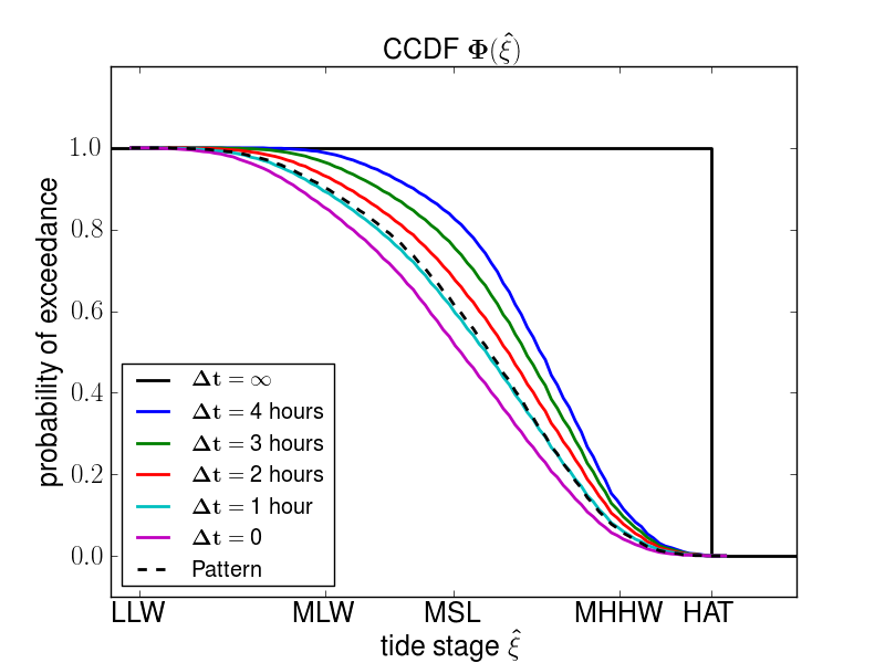
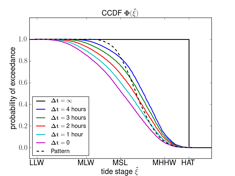
Figure 6: $\Phi(\hat{\xi})$ Comparisons. Left: AASZe03, Right: AASZe02

5.4 G and Pattern $\Phi$ comparisons at Gauge 101 for AASZe03

We ran the Pattern Method on the 5-day proxy tsunami that is assumed by the G Method and compared the resulting $\Phi$ functions at Gauge 101. The amplitude for the 5-day proxy tsunami was taken as that of the biggest wave seen at Gauge 101 for AASZe03. The two distributions when plotted are almost identical with values differing mostly less than 1% as seen in Figure 7 as the green and dashed red graphs and given in the first line of Table 2. The black graph is the distribution for the Pattern Method on the actual tsumani at Gauge 101 for which we used a $T=267$ minute duration. The blue graph shows the Pattern Method assuming a 267 minute proxy tsunami which shows differences in the proxy and actual tsunami patterns.

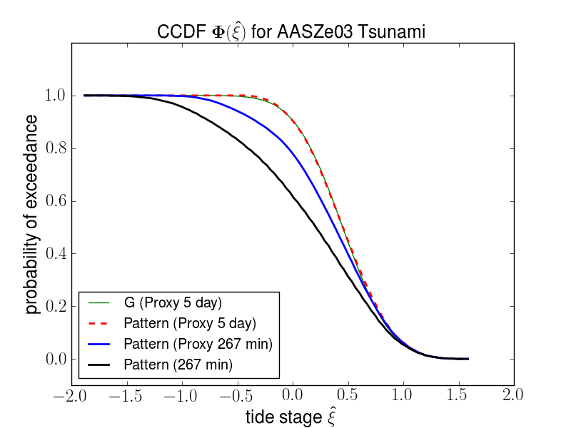
Figure 7: Pattern Method Validation

This explains that differences in $\Phi$ for any real tsunami are not due to our methodology, but to the fact that the real tsunami is not well approximated by the proxy one, even if we enforce both to have the same time duration.

5.5 Probability differences

For each grid location, we compared the 35 probabilities $P(\zeta>\zeta_{i})$ of the three methods for AASZe03. The numbers in Table 3 are over all the grid locations that cover the Crescent City area. The row labelled max is the maximum difference seen when the method being compared to the Pattern Method gives the larger result, and the row labelled min is the difference seen when the Pattern Method gives the larger result. Indeed, differences close to 1 are observed in the first column and the second column shows that the $\Delta t$ Method (with $\Delta t=1$) gives results very close to those of the Pattern Method.

Table 3: Probability Differences

	G - Pattern	$\Delta t$ - Pattern
max	+0.747	+0.006
min	-0.936	-0.017

Both the $\Delta t$ and Pattern Methods use the amplitude of the tsunami at Gauge 101 and assume its duration is T minutes instead of 5 days. Further analysis given in (Adams et al, 2013) shows that almost all of the -0.936 is due to the G Method’s choice of 5 days, while all but 0.158 of the 0.747 is due to this choice. This remaining 0.158 difference is due to the use of a proxy decaying e-folding pattern of 2 days for the tsunami, rather than the observed pattern.

In Figure 8 we compare the $\Delta t$ Method and the G Method to the Pattern Method by giving contour plots of the absolute value of the probability differences of exceeding $\zeta_{i}=0$ meters and $\zeta_{i}=2$ meters. The brighter colors in the plots indicate where these probabilities differ the most. As expected from Table 3, the $\Delta t$ and Pattern Methods differ less than 2%.

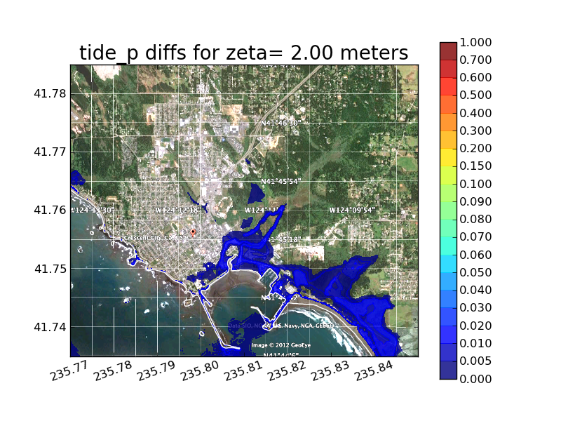
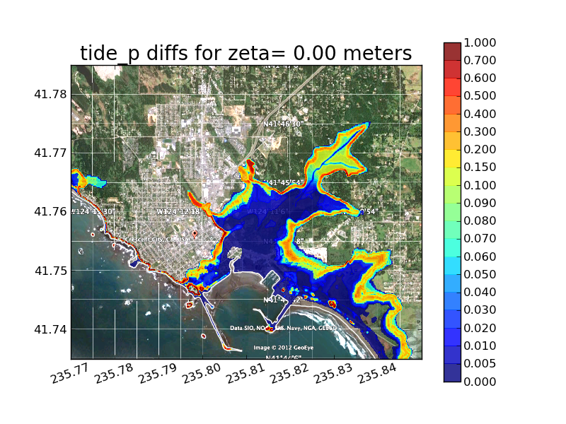
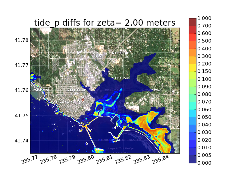
Figure 8: $P(\zeta>\zeta_{i})$ Difference Contours, Left: $\zeta_{i}=0$ m., Right: $\zeta_{i}=2$ m. Top: abs($\Delta t$ - Pattern), Bottom: abs(G - Pattern)

6 Conclusions and open questions

The $\Delta t$ Method and the Pattern Method give quite similar results for a properly chosen $\Delta t$ but vary significantly from the G Method, especially at land points. The Pattern Method is a very robust method coupled to the wave pattern for each individual tsunami and gives modelers a single method that can be used for both land and water locations. Both these methods were designed to use GeoClaw simulation information at multiple but static tidal levels, and will work with other codes that have the capability to produce similar results.

We do not model the currents that are generated by the tide rising and falling. A tsunami wave arriving on top of an incoming tide could potentially inundate further than the same amplitude wave moving against the tidal current, even if the tide stage is the same. Modeling this is beyond the scope of current tsunami models.

References

- Adams et al (2013) Adams L, LeVeque R, González FI (2013) Incorporating tidal uncertainty into probabilistic tsunami hazard assessment (ptha) for Crescent City, CA. Final Tidal Report for Phase I PTHA of Crescent City, CA, supported by FEMA Risk MAP Program, http://faculty.washington.edu/lma3/AGU2013
- Androsov et al (2011) Androsov A, Behrens J, Danilov S (2011) Tsunami modelling with unstructured grids. interaction between tides and tsunami waves. In: Computational Science and High Performance Computing IV, Springer, pp 191–206, URL http://link.springer.com/chapter/10.1007/978-3-642-17770-5_15
- Berger et al (2010) Berger MJ, George DL, LeVeque RJ, Mandli KT (2010) The geoclaw software for depth-averaged flows with adaptive refinement. Preprint and simulations: www.clawpack.org/links/papers/awr10
- González et al (2009) González FI, Geist EL, Jaffe B, Kanoglu U, et al (2009) Probabilistic tsunami hazard assessment at Seaside, Oregon, for near-and far-field seismic sources. J Geophys Res 114:C11,023
- González et al (2013) González FI, LeVeque RJ, Adams L (2013) Probabilistic tsunami hazard assessment (ptha) for Crescent City, CA, Final Report on Phase 1. http://hdl.handle.net/1773/22366