Simple single field inflation models and the running of spectral index

Abstract

The BICEP2 experiment confirms the existence of primordial gravitational wave with the tensor-to-scalar ratio $r=0$ ruled out at $7\sigma$ level. The consistency of this large value of $r$ with the Planck data requires a large negative running $n^{\prime}_{s}$ of the scalar spectral index. Herein we propose two types of the single field inflation models with simple potentials to study the possibility of the consistency of the models with the BICEP2 and Planck observations. One type of model suggested herein is realized in the supergravity model building. These models fail to provide the needed $n^{\prime}_{s}$ even though both can fit the tensor-to-scalar ratio and spectral index.

I Introduction

The observed temperature fluctuations in the cosmic microwave background radiation (CMB) strongly suggested that our Universe might experience an accelerated expansion, more precisely, inflation starobinskyfr ; guth81 ; linde83 ; Albrecht:1982wi , at a seminal stage of evolution. In addition to the solution to the problems in the standard big bang cosmology such as the flatness, horizon, and monopole problems, the inflation models predict the cosmological perturbations in the matter density from the inflaton vacuum fluctuations, which describes the primordial power spectrum consistently. Besides the scalar perturbation, the tensor perturbation is generated as well, which gives the B-mode polarisation as a signature of the primordial gravitational wave.

Recently, the BICEP2 experiment has discovered the primordial gravitational wave with the B-mode power spectrum around $\ell\sim 80$ Ade:2014xna . If it is confirmed, it will seemingly forward the study in fundamental physics. BICEP2 experiment Ade:2014xna has measured the tensor-to-scalar ratio to be $r=0.20^{+0.07}_{-0.05}$ at the 68% confidence level for the lensed-$\Lambda$CDM model, with $r=0$ disfavoured at $7.0\sigma$ level. Subtracting the various dust models and re-deriving the $r$ constraint still results in high significance of detection, it results in $r=0.16^{+0.06}_{-0.05}$. From the first-year observations, the Planck temperature power spectrum planck13 in combination with the nine years of Wilkinson Microwave Anisotropy Probe (WMAP) polarization low-multipole likelihood wmap9 and the high-multipole spectra from the Atacama Cosmology Telescope (ACT) act13 and the South Pole Telescope (SPT) spt11 (Planck+WP+highL) constrained the tensor-to-scalar ratio to be $r\leq 0.11$ at the 95% confidence level Ade:2013zuv ; Ade:2013uln . Therefore, the BICEP2 result is in disagreement with the Planck result. To reduce the inconsistency between Planck and BICEP2 experiments, we need to include the running of the spectral index $n^{\prime}_{s}=d\ln n_{s}/d\ln k$. With the running of the spectral index, the 68% constraints from the Planck+WP+highL data are $n_{s}=0.9570\pm 0.0075$ and $n^{\prime}_{s}=-0.022\pm 0.010$ with $r<0.26$ at the 95% confidence level. Thus, the running of the spectral index needs to be smaller than 0.008 at the 3$\sigma$ level for any viable inflation model.

Because different inflationary models predict different magnitudes for the tensor perturbations, such large tensor-to-scalar ratio $r$ from the BICEP2 measurement will give a strong constraint on the inflation models. Also, the inflaton potential is around the Grand Unified Theory (GUT) scale $2\times 10^{16}$ GeV, and Hubble scale is about $1.0\times 10^{14}$ GeV. From the naive analysis of Lyth bound Lyth:1996im , a large field inflation will be experienced, and then the validity of effective field theory will be challenged since the high-dimensional operators are suppressed by the reduced Planck scale. The inflation models, which can have $n_{s}\simeq 0.96$ and $r\simeq 0.16/0.20$, have been studied extensively Anchordoqui:2014uua ; Czerny:2014wua ; Ferrara:2014ima ; Zhu:2014wda ; Gong:2014cqa ; Okada:2014lxa ; Ellis:2014rxa ; Antusch:2014cpa ; Freivogel:2014hca ; Bousso:2014jca ; Kaloper:2014zba ; Choudhury:2014kma ; *Choudhury:2014wsa; *Choudhury:2013iaa; *Choudhury:2014kma; Choi:2014aca ; Murayama:2014saa ; McDonald:2014oza ; Gao:2014fha ; Ashoorioon:2014nta ; *Ashoorioon:2013eia; *Ashoorioon:2009wa; *Ashoorioon:2011ki; Sloth:2014sga ; Kawai:2014doa ; Kobayashi:2014rla ; *Kobayashi:2014ooa; *Kobayashi:2014jga; Bastero-Gil:2014oga ; DiBari:2014oja ; Ho:2014xza ; Hotchkiss:2011gz . Specifically, the simple chaotic and natural inflation models are preferred.

Conversely, supersymmetry is the most promising extension for the particle physics Standard Model (SM). Specifically, it can stabilize the scalar masses, and has a non-renormalized superpotential. Also, gravity is critical in the early Universe, so it seems to us that supergravity theory is a natural framework for inflation model building Freedman:1976xh ; *Deser:1976eh; Antusch:2009ty ; *Antusch:2011ei. However, supersymmetry breaking scalar masses in a generic supergravity theory are of the same order as the gravitino mass, inducing the reputed $\eta$ problem Copeland:1994vg ; *Stewart:1994ts; *adlinde90; *Antusch:2008pn; *Yamaguchi:2011kg; *Martin:2013tda; Lyth:1998xn , where all the scalar masses are of the order of the Hubble parameter because of the large vacuum energy density during inflation Goncharov:1984qm . There are two elegant solutions: no-scale supergravity Cremmer:1983bf ; *Ellis:1983sf; *Ellis:1983ei; *Ellis:1984bm; *Lahanas:1986uc; Ellis:1984bf ; Enqvist:1985yc ; Ellis:2013xoa ; Ellis:2013nxa ; Li:2013moa ; Ellis:2013nka , and shift-symmetry in the Kähler potential Kawasaki:2000yn ; Yamaguchi:2000vm ; Yamaguchi:2001pw ; Kawasaki:2001as ; Kallosh:2010ug ; Kallosh:2010xz ; Nakayama:2013jka ; Nakayama:2013txa ; Takahashi:2013cxa ; Li:2013nfa .

Thus, three issues need to be addressed regarding the criteria of the inflation model building:

Firstly (C-1), the spectral index is around 0.96, and the tensor-to-scalar ratio is around 0.16/0.20.

Secondly (C-2), to reconcile the Planck and BICEP2 results, we need to have $n^{\prime}_{s}\sim-0.22$. For simplicity, we do not consider the alternative approach here Freivogel:2014hca ; Bousso:2014jca .

Lastly (C-3), we need to violate the Lyth bound and try to realize the sub-Planckian inflation. For simplicity, we will not consider the alternative mechanisms such as two-field inflation models Hebecker:2013zda ; McDonald:2014oza , and the models which employ symmetries to control the quantum corrections like the axion monodromy McAllister:2008hb .

It seemingly appears that (C-1) can be satisfied by a considerable amount of inflaton potentials, thus, this is not a difficulty to overcome. In this paper, we will propose two types of the simple single field inflation models, and show that their spectral indices and tensor-to-scalar ratios are highly consistent with both the Planck and BICEP2 experiments. We construct one type of inflation models from the supergravity theory with shift symmetry in the Kähler potential. However, in these simple inflation models, we will show that (C-2) and (C-3) can not be satisfied.

II Slow-roll Inflation

The slow-roll parameters are defined as

$$\epsilon=\frac{M_{pl}^{2}V_{\phi}^{2}}{2V^{2}},$$ (1)

$$\eta=\frac{M_{pl}^{2}V_{\phi\phi}}{V},$$ (2)

$$\xi^{2}=\frac{M_{pl}^{4}V_{\phi}V_{\phi\phi\phi}}{V^{2}},$$ (3)

where $M^{2}_{pl}=(8\pi G)^{-1}$, $V_{\phi}=dV(\phi)/d\phi$, $V_{\phi\phi}=d^{2}V(\phi)/d\phi^{2}$ and $V_{\phi\phi\phi}=d^{3}V(\phi)/d\phi^{3}$. For the single field inflation, the scalar power spectrum is

$$\mathcal{P}_{\mathcal{R}}=A_{s}\left(\frac{k}{k_{*}}\right)^{n_{s}-1+n_{s}^{\prime}\ln(k/k_{*})/2},$$ (4)

where the subscript ”*” means the value at the horizon crossing, the scalar amplitude is thus

$$A_{s}\approx\frac{1}{24\pi^{2}M^{4}_{pl}}\frac{\Lambda^{4}}{\epsilon},$$ (5)

the scalar spectral index and the running are given Lyth:1998xn ; Stewart:1993bc by

$$\begin{split}n_{s}\approx 1+2\eta-6\epsilon+2\left[\frac{1}{3}\eta^{2}+(8C-1)\epsilon\eta\right.\\ \left.-\left(\frac{5}{3}+12C\right)\epsilon^{2}-\left(C-\frac{1}{3}\right)\xi^{2}\right],\end{split}$$ (6)

$$n_{s}^{\prime}=16\epsilon\eta-24\epsilon^{2}-2\xi^{2},$$ (7)

where $C=-2+\ln 2+\gamma\simeq-0.73$ with $\gamma$ the Euler-Mascheroni constant. The tensor power spectrum is

$$\mathcal{P}_{T}=A_{T}\left(\frac{k}{k_{*}}\right)^{n_{t}},$$ (8)

the tensor spectral index and the tensor to scalar ratio Lyth:1998xn ; Stewart:1993bc are

$$n_{t}=-2\epsilon\left[1+\left(4C+\frac{11}{3}\right)\epsilon-2\left(\frac{2}{3}+C\right)\eta\right]\approx-2\epsilon,$$ (9)

$$r=\frac{A_{T}}{A_{s}}=16\epsilon\left[1+8\left(C+\frac{2}{3}\right)(2\epsilon-\eta)\right]\approx 16\epsilon.$$ (10)

With the BICEP2 result $r=0.2$, the energy scale of inflation is $\Lambda\sim 2\times 10^{16}$ Gev and the slow roll parameter $\epsilon\sim 0.0125$ to the first order approximation. If $\xi^{2}\ll\epsilon$, then the second order correction for the scalar spectral index $n_{s}$ in Eq. (6) is negligible, we have

$$n^{\prime}_{s}=\frac{r(n_{s}-1)}{2}+\frac{3r^{2}}{32}-2\xi^{2}.$$ (11)

It is clear that $n_{s}^{\prime}\sim 10^{-3}$ with the observational results. Therefore, to get $n_{s}^{\prime}\sim-0.02$, we need to consider large $\xi^{2}$ and the second order correction to the scalar spectral index $n_{s}$ in Eq. (6). If $\xi^{2}\sim 0.01$, then the main contribution to the running of the spectral comes from $\xi^{2}$. For slow roll parameters $\epsilon$ and $\eta$, we have $|\epsilon|\leq 0.01$ and $|\eta|\leq 0.01$. Note that $8(C+\frac{2}{3})\simeq-0.506667$, we can neglect the term $8(C+\frac{2}{3})(2\epsilon-\eta)$ at the next leading order in Eqs. (9) and (10). Thus, we will take the leading order approximation $n_{t}=-2\epsilon$ and $r=16\epsilon$ for simplicity.

The number of e-folds before the end of inflation is given by

$$N(\phi)=\int_{t}^{t_{e}}Hdt\approx\frac{1}{M_{pl}^{2}}\int_{\phi_{e}}^{\phi}\frac{V(\phi)}{V_{\phi}(\phi)}d\phi=\frac{1}{\sqrt{2}\,M_{pl}}\int_{\phi_{e}}^{\phi}\frac{d\phi}{\sqrt{\epsilon}},$$ (12)

where the value $\phi_{e}$ of the inflaton at the end of inflation is defined by $\epsilon(\phi_{e})=1$. Now let us briefly consider the Lyth bound Lyth:1996im . From the above equation, we have

$$\Delta\phi\equiv|\phi_{*}-\phi_{e}|>{\sqrt{2\epsilon_{\rm min}}}N(\phi)M_{pl}~{},~{}\,$$ (13)

where $\epsilon_{\rm min}$ is the minimal $\epsilon$ during inflation. If $\epsilon(\phi)$ is a monotonous function of $\phi$, we have $\epsilon_{\rm min}=\epsilon(\phi_{*})\equiv\epsilon$. With the BICEP2 result $r=0.16/0.20$, we can obtain the large field inflation because of $\Delta\phi>7M_{pl}$. Thus, to violate the Lyth bound and have the magnitude of $\phi$ smaller than the reduced Planck scale during inflation, we require that $\epsilon(\phi)$ is not a monotonous function and it has a minimum between $\phi_{*}$ and $\phi_{e}$.

III Single Field Inflation Models with Simple Potentials

III.1 Inflaton Potentials

Herein, we will describe one type of the single field inflation models with simple potentials. The inflation models with potential $\alpha\phi^{n}e^{-\beta\phi^{m}}$ Li:2013nfa have been studied systematically previously, while such type of potentials may have the unlikeliness problem Ijjas:2013vea unless both $n$ and $m$ are even. Conversely, for the S-dual inflation with the potential $V(\phi)=V_{0}{\rm sech}(\phi/M)$ Anchordoqui:2014uua , the slow-roll parameters are

$$\epsilon=\frac{M^{2}_{pl}}{2M^{2}}\tanh^{2}(\phi/M),$$ (14)

$$\eta=4\epsilon-\frac{M^{2}_{pl}}{M^{2}},$$ (15)

$$\xi^{2}=24\epsilon^{2}-10\left(\frac{M_{pl}}{M}\right)^{2}\epsilon.$$ (16)

To satisfy slow-roll condition, $g=M/M_{pl}$ must be large, then $\epsilon<1$ always and inflation will not end. Thus we need another mechanism to end inflation. For the S-dual inflation, we have

$$r=16\epsilon=8g^{-2}\tanh^{2}(\phi/M)\leq 8/g^{2},$$ (17)

$$n_{s}=1+\frac{r}{8}-\frac{2}{g^{2}}\leq 1-\frac{r}{8},$$ (18)

$$n_{s}^{\prime}=\frac{r}{4}\left(\frac{1}{g^{2}}-\frac{r}{8}\right)\geq 0.$$ (19)

The number of e-folds before the end of inflation is given as

$$N(\phi)=\int_{\phi_{e}}^{\phi}\frac{g^{2}}{\tanh(\phi/M)}d\phi=g^{2}\,\ln\left[\frac{\sinh(\phi/M)}{\sinh(\phi_{e}/M)}\right].$$ (20)

If we take $\phi_{e}=M$, $g=M/M_{pl}=5.7735$ and $\phi/M=2.659$, we get $n_{s}=0.969$, $r=0.235$, $n_{s}^{\prime}=3.4\times 10^{-5}$ and $N=60$, which is marginally consistent with the observational constraint at the 95% confidence level.

Let us suggest one type of the inflation models with the hybrid monomial and S-dual potentials $V(\phi)=V_{0}\phi^{n}{\rm sech}(\phi/M)$, here $n$ is an even integer. The slow-roll parameters are

$$\epsilon=\frac{1}{2g^{2}}\left[\frac{n}{\phi/M}-\tanh(\phi/M)\right]^{2},$$ (21)

$$\eta=\frac{1}{g^{2}}\left[\frac{n(n-1)}{(\phi/M)^{2}}-\frac{2n}{\phi/M}\tanh(\phi/M)+\right.$$

$$2\tanh^{2}(\phi/M)-1],$$ (22)

$$\xi^{2}=\frac{1}{g^{4}}\left[6\tanh^{4}(\phi/M)-\frac{12n}{\phi/M}\tanh^{3}(\phi/M)+\right.$$

$$\left(\frac{9n^{2}-3n}{(\phi/M)^{2}}-5\right)\tanh^{2}(\phi/M)+$$

$$\left(\frac{8n}{\phi/M}-\frac{4n^{3}-6n^{2}+2n}{(\phi/M)^{3}}\right)\tanh(\phi/M)+$$

$$\left.\frac{n^{2}(n-1)(n-2)}{(\phi/M)^{4}}-\frac{3n^{2}}{(\phi/M)^{2}}\right].$$ (23)

So the spectral index also satisfies the bound

$$\eta=2\epsilon+g^{-2}\left[\tanh^{2}(\phi/M)-\frac{n}{(\phi/M)^{2}}-1\right]\leq 2\epsilon,$$ (24)

$$n_{s}=1+2\eta-\frac{3r}{8}\leq 1-\frac{r}{8}.$$ (25)

For $n=2$, $g=100$ and $N=60$, we obtain $\phi_{e}/M=0.0141$, $\phi/M=0.156$, $n_{s}=0.967$, $r=0.128$ and $n_{s}^{\prime}=-5.338\times 10^{-4}$. If we choose $n=4$, $g=30$ and $N=60$, we obtain $\phi_{e}/M=0.0941$, $\phi/M=0.715$, $n_{s}=0.954$, $r=0.221$ and $n_{s}^{\prime}=-7.960\times 10^{-4}$. For $n=6$, $g=10$ and $N=60$, we get $\phi_{e}/M=0.4129$, $\phi/M=2.350$, $n_{s}=0.953$, $r=0.198$ and $n_{s}^{\prime}=-8.667\times 10^{-4}$. The results for $n=2$, $n=4$ and $n=6$ are shown in Figs. 1 and 2. We also show the observational constraints. From Figs. 1 and 2, it can be seen that these models are marginally consistent with the observational results at the 95% confidence level. For $n=2$, if there is an increase of the value of $g$ or the value of the energy scale $M$, then both $r$ and $|n_{s}^{\prime}|$ increase when $n_{s}$ is retained, then the results are almost unchanged when $g\geq 100$. For $n=4$ and $n=6$, if there is an increase in $g$ and $n_{s}$ is fixed, then $r$ increases and $n_{s}^{\prime}$ moves closer to zero. At the 95% confidence level, we find that $g\geq 20$ for $n=2$, $8\leq g\leq 30$ for $n=4$ and $6\leq g\leq 10$ for $n=6$.

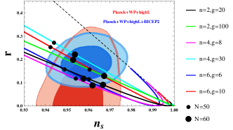
Figure 1: The $n_{s}-r$ diagrams for the potential $V(\phi)=V_{0}\phi^{n}{\rm sech}(\phi/M)$. Confidence levels of 68% and 95% confidence contour from the combinations of Planck+WP+highL Ade:2013zuv ; Ade:2013uln and Planck+WP+highL+BICEP2 data Ade:2014xna are also included.

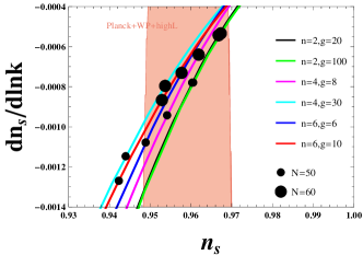
Figure 2: The $n_{s}-n_{s}^{\prime}$ diagrams for the potential $V(\phi)=V_{0}\phi^{n}{\rm sech}(\phi/M)$. Confidence level of 95% confidence contour from the combinations of Planck+WP+highL data Ade:2013zuv ; Ade:2013uln is also included.

III.2 Supergravity Model Building

For a given Kähler potential $K$ and a superpotential $W$ in the supergravity theory, we have the following scalar potential

$$V=e^{K}\left((K^{-1})^{i}_{\bar{j}}D_{i}WD^{\bar{j}}\overline{W}-3|W|^{2}\right)~{},~{}$$ (26)

where $(K^{-1})^{i}_{\bar{j}}$ is the inverse of the Kähler metric $K_{i}^{\bar{j}}=\partial^{2}K/\partial\Phi^{i}\partial{\bar{\Phi}}_{\bar{j}}$, and $D_{i}W=W_{i}+K_{i}W$. Also, the kinetic term for the scalar field is

$${\cal L}~{}=~{}K_{i}^{\bar{j}}\partial_{\mu}\Phi^{i}\partial^{\mu}{\bar{\Phi}}_{\bar{j}}~{}.~{}\,$$ (27)

Introducing two superfields $\Phi$ and $X$, we consider the following Kähler potential and superpotential

$$K=-\frac{1}{2}(\Phi+{\bar{\Phi}})^{2}+X{\bar{X}}-\delta(X{\bar{X}})^{2}~{},~{}$$ (28)

$$W~{}=~{}Xf(\Phi)~{}.~{}\,$$ (29)

Therefore, the Kähler potential $K$ is invariant under the following shift symmetry Kawasaki:2000yn ; Yamaguchi:2000vm ; Yamaguchi:2001pw ; Kawasaki:2001as ; Kallosh:2010ug ; Kallosh:2010xz ; Nakayama:2013jka ; Nakayama:2013txa ; Takahashi:2013cxa ; Li:2013nfa is thus

$$\Phi\rightarrow\Phi+iCM_{pl}~{},~{}\,$$ (30)

with $C$ a dimensionless real parameter. In general, the Kähler potential $K$ is a function of $\Phi+\Phi^{\dagger}$ and independent on the imaginary part of $\Phi$.

We can obtain the scalar potential as follows

$$V = e^{K}\left[|(\Phi+{\bar{\Phi}})Xf(\Phi)+X\frac{\partial f(\Phi)}{\partial\Phi}|^{2}-3|Xf(\Phi)|^{2}\right.$$ (31)

$$\left.+|({\bar{X}}-2\delta X{\bar{X}}^{2})Xf(\Phi)+f(\Phi)|^{2}\right]~{}.~{}\,$$

Because there is no imaginary component ${\rm Im}[\Phi]$ of $\Phi$ in the Kähler potential because of the shift symmetry, the potential along ${\rm Im}[\Phi]$ is considerably flat and then ${\rm Im}[\Phi]$ is a natural inflaton candidate. From the previous studies Kallosh:2010ug ; Kallosh:2010xz ; Li:2013nfa , the real component ${\rm Re}[\Phi]$ of $\Phi$ and $X$ can be stabilized at the origin during inflation, i.e., ${\rm Re}[\Phi]=0$ and $X=0$. Therefore, with ${\rm Im}[\Phi]=\phi/{\sqrt{2}}$, we obtain the inflaton potential

$$V~{}=~{}|f(\phi/{\sqrt{2}})|^{2}~{}.~{}\,$$ (32)

If we chosse $f(\Phi)$ as below

$$f(\Phi)~{}=~{}\frac{{\sqrt{V}_{0}}({\sqrt{2}}\Phi/M)^{m}}{e^{-i\Phi/{\sqrt{2}}M}+e^{i\Phi/{\sqrt{2}}M}}~{},~{}\,$$ (33)

with $m$ a positive integer, we realize the potential $V(\phi)=V_{0}\phi^{n}{\rm sech^{2}}(\phi/M)$ with $n=2m$. The slow-roll parameters for this type of models are

$$\epsilon=\frac{1}{2g^{2}}\left[\frac{n}{\phi/M}-2\tanh(\phi/M)\right]^{2},$$ (34)

$$\eta=\frac{1}{g^{2}}\left[\frac{n(n-1)}{(\phi/M)^{2}}-2{\rm sech^{2}}(\phi/M)+4\tanh^{2}(\phi/M)\right.$$

$$\left.-\frac{4n}{\phi/M}\tanh(\phi/M)\right],$$ (35)

$$\xi^{2}=\frac{1}{g^{4}}\left[\frac{n}{\phi/M}-2\tanh(\phi/M)\right]\times\left[\frac{n(2-3n+n^{2})}{(\phi/M)^{3}}-\right.$$

$$\frac{6n(n-1)}{(\phi/M)^{2}}\tanh(\phi/M)+\frac{12n}{\phi/M}\tanh^{2}(\phi/M)-8\tanh^{3}(\phi/M)+$$

$$\left.2{\rm sech^{2}}(\phi/M)(8\tanh(\phi/M)-\frac{3n}{\phi/M})\right].$$ (36)

Thus the spectral index also satisfies the bound

$$\eta=2\epsilon-g^{-2}\left[2{\rm sech^{2}}(\phi/M)+\frac{n}{(\phi/M)^{2}}\right]\leq 2\epsilon,$$ (37)

$$n_{s}=1+2\eta-\frac{3r}{8}\leq 1-\frac{r}{8}.$$ (38)

For $n=2$, $g=100$, and $N=60$, we obtain $\phi_{e}/M=0.0141$, $\phi/M=0.155$, $n_{s}=0.967$, $r=0.127$ and $n_{s}^{\prime}=-5.411\times 10^{-4}$. If we take $n=4$, $g=30$ and $N=60$, then we obtain $\phi_{e}/M=0.0939$, $\phi/M=0.694$, $n_{s}=0.956$, $r=0.185$ and $n_{s}^{\prime}=-7.795\times 10^{-4}$. For $n=6$, $g=10$ and $N=60$, we obtain $\phi_{e}/M=0.4025$, $\phi/M=2.030$, $n_{s}=0.958$, $r=0.084$ and $n_{s}^{\prime}=-6.794\times 10^{-4}$. The results for $n=2$, $n=4$ and $n=6$ are shown in Figs. 3 and 4. We also show the observational constraints. From Figs. 3 and 4, it can be seen from the models that they are also marginally consistent with the observational results at the 95% confidence level. For $n=2$, if $n_{s}$ is fixed and increase the value of $g$ or the value of the energy scale $M$, then both $r$ and $|n_{s}^{\prime}|$ increase, with the result almost unchanged when $g\geq 100$. For $n=4$ and $n=6$, if we increase $g$ and retain $n_{s}$ fixed, then $r$ increases and $n_{s}^{\prime}$ moves closer to zero. At the 95% confidence level, we find that $g\geq 30$ for $n=2$, $15\leq g\leq 30$ for $n=4$ and $g\sim 10$ for $n=6$.

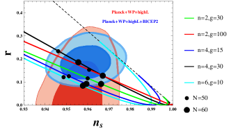
Figure 3: The $n_{s}-r$ diagrams for the potential $V(\phi)=V_{0}\phi^{n}{\rm sech^{2}}(\phi/M)$. Confidence levels of 68% and 95% confidence contours from the combinations of Planck+WP+highL Ade:2013zuv ; Ade:2013uln and Planck+WP+highL+BICEP2 data Ade:2014xna are also included.

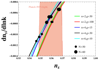
Figure 4: The $n_{s}-n_{s}^{\prime}$ diagrams for the potential $V(\phi)=V_{0}\phi^{n}{\rm sech^{2}}(\phi/M)$. Confidence level of 95% confidence contour from the combinations of Planck+WP+highL data Ade:2013zuv ; Ade:2013uln is also included.

IV Discussion

Herein we have proposed one type of the single field inflation models with the hybrid monomial and S-dual potentials $V(\phi)=V_{0}\phi^{n}{\rm sech}(\phi/M)$ and found that $n_{s}^{\prime}$ given by the model is around $-10^{-4}$ when $n_{s}$ and $r$ are consistent with the BICEP2 constraints. If we increase the model parameter $n$ or $g=M/M_{pl}$, for the same value of $n_{s}$, then the tensor-to-scalar ratio $r$ increases, but the running of the scalar spectral index $n_{s}^{\prime}$ moves closer to zero except for $n=2$. Therefore, the model parameters are constrained by the observational results. At the 95% confidence level, we obtained that $g\geq 20$ for $n=2$, $8\leq g\leq 30$ for $n=4$ and $6\leq g\leq 10$ for $n=6$.

Then we used the supergravity model building method to propose another type of models with the potentials $V(\phi)=V_{0}\phi^{n}{\rm sech}^{2}(\phi/M)$. The behavior of this model is similar to the inflation model with the potential $V(\phi)=V_{0}\phi^{n}{\rm sech}(\phi/M)$ and the model is more constrained by the observational data. At the 95% confidence level, we found that $g\geq 30$ for $n=2$, $15\leq g\leq 30$ for $n=4$ and $g\sim 10$ for $n=6$. The running of the scalar spectral index for both models is at the order of $-10^{-4}$. Both models failed to provide the second order slow-roll parameter $\xi^{2}$ as large as the first order slow-roll parameters $\epsilon$ and $\eta$. Furthermore, to obtain large $r$, the inflaton will experience a Planck excursion because of the Lyth bound. This is the common problem for single field inflation as suggested by Gong  Gong:2014cqa . To violate the Lyth bound and result in sub-Planckian inflaton field, the slow roll parameter $\epsilon$ needs not be retained by a monotonous function during inflation Hotchkiss:2011gz ; BenDayan:2009kv . Recently Ben-Dayan and Brustein  BenDayan:2009kv found that $n_{s}=0.96$, $r=0.1$ and $n_{s}^{\prime}=-0.07$ for a single field inflation with polynomial potential. It remains unclear if a single field inflation model can be constructed which both contain a large $r$ and $n_{s}^{\prime}$.

- (1) A. A. Starobinsky, Phys. Lett. B. 91 (1980) 99.
- (2) A. H. Guth, Phys. Rev. D 23 (1981) 347.
- (3) A. D. Linde, Phys. Lett. B 129 (1983) 177.
- (4) A. Albrecht and P. J. Steinhardt, Phys. Rev. Lett. 48 (1982) 1220.
- (5) P. Ade et al., BICEP2 I: Detection Of B-mode Polarization at Degree Angular Scales, arXiv:1403.3985 [astro-ph.CO], 2014.
- (6) P. Ade et al., Planck 2013 results. I. Overview of products and scientific results, arXiv:1303.5062 [astro-ph.CO], 2013.
- (7) G. Hinshaw et al., Astrophys. J. Suppl. 208 (2013) 19 (arXiv: 1212.5226).
- (8) S. Das et al., JCAP 1404 (2014) 014.
- (9) R. Keisler et al., Astrophys. J. 743 (2011) 28.
- (10) P. Ade et al., Planck 2013 results. XVI. Cosmological parameters, arXiv:1303.5076 [astro-ph.CO], 2013.
- (11) P. Ade et al., Planck 2013 results. XXII. Constraints on inflation, arXiv:1303.5082 [astro-ph.CO], 2013.
- (12) D. H. Lyth, Phys. Rev. Lett. 78 (1997) 1861.
- (13) L. A. Anchordoqui, V. Barger, H. Goldberg, X. Huang, and D. Marfatia, Phys. Lett. B 734 (2014) 134.
- (14) M. Czerny, T. Kobayashi, and F. Takahashi, Running Spectral Index from Large-field Inflation with Modulations Revisited, arXiv:1403.4589 [astro-ph.CO], 2014.
- (15) S. Ferrara, A. Kehagias, and A. Riotto, The Imaginary Starobinsky Model, arXiv:1403.5531 [hep-th], 2014.
- (16) T. Zhu and A. Wang, Gravitational quantum effects in the light of BICEP2 results, arXiv:1403.7696 [astro-ph.CO], 2014.
- (17) Q. Gao and Y. Gong, Phys. Lett. B 734 (2014) 41.
- (18) N. Okada, V. N. , and Q. Shafi, Simple Inflationary Models in Light of BICEP2: an Update, arXiv:1403.6403 [hep-ph], 2014.
- (19) J. Ellis, M. A. G. Garcia, D. V. Nanopoulos, and K. A. Olive, Resurrecting Quadratic Inflation in No-Scale Supergravity in Light of BICEP2, arXiv:1403.7518 [hep-ph], 2014.
- (20) S. Antusch and D. Nolde, JCAP 1405 (2014) 035.
- (21) B. Freivogel, M. Kleban, M. R. Martinez, and L. Susskind, Observational Consequences of a Landscape: Epilogue, arXiv:1404.2274 [astro-ph.CO], 2014.
- (22) R. Bousso, D. Harlow, and L. Senatore, Inflation After False Vacuum Decay: New Evidence from BICEP2, arXiv:1404.2278 [astro-ph.CO], 2014.
- (23) N. Kaloper and A. Lawrence, Natural Chaotic Inflation and UV Sensitivity, arXiv:1404.2912 [hep-th], 2014.
- (24) S. Choudhury and A. Mazumdar, Reconstructing inflationary potential from BICEP2 and running of tensor modes, arXiv:1403.5549 [hep-th], 2014.
- (25) S. Choudhury and A. Mazumdar, Sub-Planckian inflation & large tensor to scalar ratio with , arXiv:1404.3398 [hep-th], 2014.
- (26) S. Choudhury and A. Mazumdar, Nucl. Phys. B 882 (2014) 386.
- (27) K.-Y. Choi and B. Kyae, Primordial gravitational wave of BICEP2 from dynamical double hybrid inflation, arXiv:1404.3756 [hep-ph], 2014.
- (28) H. Murayama, K. Nakayama, F. Takahashi, and T. T. Yanagida, Sneutrino Chaotic Inflation and Landscape, arXiv:1404.3857 [hep-ph], 2014.
- (29) J. McDonald, Sub-Planckian Two-Field Inflation Consistent with the Lyth Bound, arXiv:1404.4620 [hep-ph], 2014.
- (30) X. Gao, T. Li, and P. Shukla, Fractional chaotic inflation in the lights of PLANCK and BICEP2, arXiv:1404.5230 [hep-ph], 2014.
- (31) A. Ashoorioon, K. Dimopoulos, M. Sheikh-Jabbari, and G. Shiu, Non-Bunch-Davis Initial State Reconciles Chaotic Models with BICEP and Planck, arXiv:1403.6099 [hep-th], 2014.
- (32) A. Ashoorioon, K. Dimopoulos, M. Sheikh-Jabbari, and G. Shiu, JCAP 1402 (2014) 025.
- (33) A. Ashoorioon, H. Firouzjahi, and M. Sheikh-Jabbari, JCAP 0906 (2009) 018.
- (34) A. Ashoorioon and M. Sheikh-Jabbari, JCAP 1106 (2011) 014.
- (35) M. S. Sloth, Chaotic inflation with curvaton induced running, arXiv:1403.8051 [hep-ph], 2014.
- (36) S. Kawai and N. Okada, TeV scale seesaw from supersymmetric Higgs-lepton inflation and BICEP2, arXiv:1404.1450 [hep-ph], 2014.
- (37) T. Kobayashi and O. Seto, Beginning of Universe through large field hybrid inflation, arXiv:1404.3102 [hep-ph], 2014.
- (38) T. Kobayashi, O. Seto, and Y. Yamaguchi, Axion monodromy inflation with sinusoidal corrections, arXiv:1404.5518 [hep-ph], 2014.
- (39) T. Kobayashi and O. Seto, Phys. Rev. D 89 (2014) 103524.
- (40) M. Bastero-Gil, A. Berera, R. O. Ramos, and J. G. Rosa, Observational implications of mattergenesis during inflation, arXiv:1404.4976 [astro-ph.CO], 2014.
- (41) P. Di Bari, S. F. King, C. Luhn, A. Merle, and A. Schmidt-May, Radiative Inflation and Dark Energy RIDEs Again after BICEP2, arXiv:1404.0009 [hep-ph], 2014.
- (42) C. M. Ho and S. D. H. Hsu, Does the BICEP2 Observation of Cosmological Tensor Modes Imply an Era of Nearly Planckian Energy Densities?, arXiv:1404.0745 [hep-ph], 2014.
- (43) S. Hotchkiss, A. Mazumdar, and S. Nadathur, JCAP 1202 (2012) 008.
- (44) D. Z. Freedman, P. van Nieuwenhuizen, and S. Ferrara, Phys. Rev. D 13 (1976) 3214.
- (45) S. Deser and B. Zumino, Phys. Lett. B 62 (1976) 335.
- (46) S. Antusch, M. Bastero-Gil, K. Dutta, S. F. King, and P. M. Kostka, Phys. Lett. B 679 (2009) 428.
- (47) S. Antusch, K. Dutta, J. Erdmenger, and S. Halter, JHEP 1104 (2011) 065.
- (48) E. J. Copeland, A. R. Liddle, D. H. Lyth, E. D. Stewart, and D. Wands, Phys. Rev. D 49 (1994) 6410.
- (49) E. D. Stewart, Phys. Rev. D 51 (1995) 6847.
- (50) A. Linde, Particle Physics and Inflationary Cosmology (Harwood Academic Publishers, Chur, Switzerland and New York, 1990).
- (51) S. Antusch, M. Bastero-Gil, K. Dutta, S. F. King, and P. M. Kostka, JCAP 0901 (2009) 040.
- (52) M. Yamaguchi, Class. Quant. Grav. 28 (2011) 103001.
- (53) J. Martin, C. Ringeval, and V. Vennin, Encyclopaedia Inflationaris, arXiv:1303.3787 [astro-ph.CO], 2013.
- (54) D. H. Lyth and A. Riotto, Phys. Rept. 314 (1999) 1.
- (55) A. S. Goncharov, A. D. Linde, and M. I. Vysotsky, Phys. Lett. B 147 (1984) 279.
- (56) E. Cremmer, S. Ferrara, C. Kounnas, and D. V. Nanopoulos, Phys. Lett. B 133 (1983) 61.
- (57) J. R. Ellis, A. Lahanas, D. V. Nanopoulos, and K. Tamvakis, Phys. Lett. B 134 (1984) 429.
- (58) J. R. Ellis, C. Kounnas, and D. V. Nanopoulos, Nucl. Phys. B 241 (1984) 406.
- (59) J. R. Ellis, C. Kounnas, and D. V. Nanopoulos, Nucl. Phys. B 247 (1984) 373.
- (60) A. Lahanas and D. V. Nanopoulos, Phys. Rept. 145 (1987) 1.
- (61) J. R. Ellis, K. Enqvist, D. V. Nanopoulos, K. A. Olive, and M. Srednicki, Phys. Lett. B 152 (1985) 175 (Erratum-ibid. 156 (1985) 452).
- (62) K. Enqvist, D. V. Nanopoulos, and M. Quiros, Phys. Lett. B 159 (1985) 249.
- (63) J. Ellis, D. V. Nanopoulos, and K. A. Olive, Phys. Rev. Lett. 111 (2013) 111301 (Erratum-ibid. 111 (2013) 12, 129902).
- (64) J. Ellis, D. V. Nanopoulos, and K. A. Olive, JCAP 1310 (2013) 009.
- (65) T. Li, Z. Li, and D. V. Nanopoulos, JCAP 1404 (2014) 018.
- (66) J. Ellis, D. V. Nanopoulos, and K. A. Olive, Phys. Rev. D 89 (2014) 043502.
- (67) M. Kawasaki, M. Yamaguchi, and T. Yanagida, Phys. Rev. Lett. 85 (2000) 3572.
- (68) M. Yamaguchi and J. Yokoyama, Phys. Rev. D 63 (2001) 043506.
- (69) M. Yamaguchi, Phys. Rev. D 64 (2001) 063502.
- (70) M. Kawasaki and M. Yamaguchi, Phys. Rev. D 65 (2002) 103518.
- (71) R. Kallosh and A. Linde, JCAP 1011 (2010) 011.
- (72) R. Kallosh, A. Linde, and T. Rube, Phys. Rev. D 83 (2011) 043507.
- (73) K. Nakayama, F. Takahashi, and T. T. Yanagida, Phys. Lett. B 725 (2013) 111.
- (74) K. Nakayama, F. Takahashi, and T. T. Yanagida, JCAP 1308 (2013) 038.
- (75) F. Takahashi, Phys. Lett. B 727 (2013) 21.
- (76) T. Li, Z. Li, and D. V. Nanopoulos, JCAP 1402 (2014) 028.
- (77) A. Hebecker, S. C. Kraus, and A. Westphal, Phys. Rev. D 88 (2013) 123506.
- (78) L. McAllister, E. Silverstein, and A. Westphal, Phys. Rev. D 82 (2010) 046003.
- (79) E. D. Stewart and D. H. Lyth, Phys. Lett. B 302 (1993) 171.
- (80) A. Ijjas, P. J. Steinhardt, and A. Loeb, Phys. Lett. B 723 (2013) 261.
- (81) I. Ben-Dayan and R. Brustein, JCAP 1009 (2010) 007.