SReach: A Bounded Model Checker for Stochastic
Hybrid Systems

Abstract

In this paper we describe a new tool, SReach, which solves probabilistic bounded reachability problems for two classes of stochastic hybrid systems. The first one is (nonlinear) hybrid automata with parametric uncertainty. The second one is probabilistic hybrid automata with additional randomness for both transition probabilities and variable resets. Standard approaches to reachability problems for linear hybrid systems require numerical solutions for large optimization problems, and become infeasible for systems involving both nonlinear dynamics over the reals and stochasticity. Our approach encodes stochastic information by using random variables, and combines the randomized sampling, a $\delta$-complete decision procedure, and statistical tests. SReach utilizes the $\delta$-complete decision procedure to solve reachability problems in a sound manner, i.e., it always decides correctly if, for a given assignment to all random variables, the system actually reaches the unsafe region. The statistical tests adapted guarantee arbitrary small error bounds between probabilities estimated by SReach and real ones. Compared to standard simulation-based methods, our approach supports non-deterministic branching, increases the coverage of simulation, and avoids the zero-crossing problem. We demonstrate our method’s feasibility by applying SReach to three representative biological models and to additional benchmarks for nonlinear hybrid systems with multiple probabilistic system parameters.

1 Introduction

Stochastic hybrid systems (SHSs) are dynamical systems exhibiting discrete, continuous, and stochastic dynamics. Due to their generality, SHSs have been widely used in various areas, including cyber-physical systems, financial decision problems, and biological systems [7, 11]. The popularity of SHSs in real-world applications motivates researchers to put a significant effort into analysis methods for this class of systems. One of the elementary questions for the quantitative analysis of SHSs is the probabilistic reachability problem, i.e., computing the probability of reaching a certain set of states. The set may represent unsafe states which should be avoided or visited only with some small probability, or dually, good states which should be visited frequently. There are two reasons why this kind of problem catches the researchers’ attention. One is that most temporal properties can be reduced to reachability problems, considering the very expressive hybrid modeling framework. The other is that probabilistic state reachability is a hard and challenging problem which is undecidable in general.

To describe stochastic dynamics, uncertainties have been added to hybrid systems in a number of different ways. One of the simplest ways replaces some of the system parameters with random variables, resulting in general hybrid automata (GHAs) with parametric uncertainty. Another approach integrates deterministic flows with probabilistic jumps. When state changes forced by continuous dynamics involve discrete random events, we refer to such systems as probabilistic hybrid automata (PHAs) [30]. When state changes also involve continuous probabilistic events, we call this kind of models stochastic hybrid automata (SHAs) [15]. Other models describe randomness by substituting deterministic flows with stochastic ones, such as stochastic differential equations (SDEs) [5], where the random perturbation affects the dynamics continuously. When all such modifications have been applied, the resulting models are called general stochastic hybrid systems (GSHSs) [23]. Among these different models, of particular interest for this paper are GHAs with parametric uncertainty and PHAs with additional randomness for both transition probabilities and variable resets.

When modeling real-world systems using hybrid models, parametric uncertainty arises naturally. Although its cause is multifaceted, two factors are critical. First, probabilistic parameters are needed when the physics controlling the system is known, but some parameters are either not known precisely, are expected to vary because of individual differences, or may change by the end of the system’s operational lifetime. Second, system uncertainty may occur when the model is constructed directly from experimental data. Due to imprecise experimental measurements, the values of system parameters may have ranges of variation with some associated likelihood of occurrence. Clearly, the GHAs with parametric uncertainty are suitable models considering these major causes. Note that, in both cases, we assume that the probability distributions of probabilistic system parameters are known. Another interesting and more expressive class of models is PHAs, which extends hybrid automata [21] with discrete probability distributions. More precisely, for discrete transitions in a model, instead of making a purely nondeterministic choice over the set of currently enabled jumps, a PHA nondeterministically chooses among the set of recently enabled discrete probability distributions, each of which is defined over a set of transitions. Although randomness is defined to only influence the discrete dynamics of the model, PHAs are still very useful and have interesting practical applications [31]. In this paper, we consider a variation of PHAs, where additional randomness for both transition probabilities and resets of some system variables are allowed. In other words, in terms of the randomness for jump probabilities, we mean that the probabilities attached to probabilistic jumps from one mode, instead of having a discrete distribution with predefined constant probabilities, can be expressed by equations involving random variables whose distributions can be either discrete or continuous. This extension is motivated by the fact that some transition probabilities can vary due to factors such as individual and environmental differences in real-world systems. When it comes to the randomness of variable resets, we allow that a system variable can be reset to a value obtained according to a known discrete or continuous distribution, instead of being assigned with a fixed value. For example, with this extension, on a discrete update, variable $t$ can be assigned to any value between $1$ and $2$ with equal probability.

In this paper, we describe our tool SReach which supports probabilistic bounded reachability analysis for these two interesting model classes: GHAs with parametric uncertainty and PHAs with additional randomness. It combines the recently proposed $\delta$-complete bounded reachability analysis technique [17] with statistical testing techniques. Our technique saves the virtues of the Satisfiability Modulo Theories (SMT) based Bounded Model Checking (BMC) for GHAs [12, 33], namely the fully symbolic treatment of hybrid state spaces, while advancing the reasoning power to probabilistic models and requirements. By utilizing the $\delta$-complete analysis method, the full nondeterminism of models can be considered. By adapting statistical tests, SReach can place arbitrarily small error bounds on the estimated probabilities. Compared to standard simulation-based approaches, our approach supports nondeterministic branching, increases the coverage of simulation, and avoids the zero-crossing problem which is critical for simulation-based methods. Comparing to the existing tools introduced in [36, 16, 13, 25], besides offering a sound way to analyze nonlinear dynamics within the SHSs, SReach also supports probabilistic bounded reachability analysis for hybrid systems with parametric uncertainty. With this modeling formalism, important elements such as probabilistic initial conditions and random variable coefficients can all be expressed by multiple random variables. Furthermore, for PHAs, SReach considers a more general and useful formalism where general randomness for transition probabilities and variable resets are allowed. We discuss three biological models - a cardiac atrial fibrillation model, a prostate cancer treatment model, and our synthesized Killerred biological model - to show how SReach can be used to answer several types of questions including model validation, parameter estimation, and sensitivity analysis. To further demonstrate the feasibility of SReach, we also apply it to additional real-world hybrid systems with parametric uncertainty, e.g. the quadcopter stabilization control.

Related Work. Analysis approaches for GSHSs are often based on Monte-Carlo simulation [6]. Considering the difficulty in dealing with this general case, efforts have been mainly placed on different subclasses. For PHAs, Zhang et al. [36] abstracted the original PHA to a probabilistic automaton (PA), and then used established Model Checking methods (e.g. PRISM [25]) for the abstracted model. Hahn et al. also discussed an abstraction-based method where the given PHA was translated into a $n$-player stochastic game using two different abstraction techniques [20]. Another method proposed is an SMT-based BMC procedure [16]. In [4, 1, 2, 3], a similar class of models called discrete-time stochastic hybrid systems (DTSHSs), which is widely used in control theory, was considered. With regard to system analysis, the control problem is to find an optimal control strategy that minimizes the probability of reaching unsafe states. Zuliani et al. also mentioned a simulation-based method for model checking DTSHSs against bounded temporal properties [37]. We refer to this method as Statistical Model Checking (StatMC). Although StatMC does not belong to the class of exhaustive state-space exploration methods, it usually returns results faster than the exhaustive search with a predefined arbitrarily small error bound on the estimated probability. StatMC was recently integrated into UPPAAL [27] in order to handle very general networks of SHAs [13]. To analyze reachability problems of SHAs, Fränzle et al. [15] first over-approximated a given SHA by a PHA, and then exploited the verification procedure introduced in [36] to model check the over-approximating PHA. Plazter introduced another interesting modeling formalism - stochastic hybrid programs (SHPs) in [29]. To specify system properties, Platzer proposed a logic called stochastic differential dynamic logic, and then suggested a proof calculus to verify logical properties of SHPs.

The paper proceeds by first, in Section 2, introducing two modeling formalisms of SHSs under consideration: GHAs with parametric uncertainty, and PHAs with additional randomness. Section 3 explains how SReach solves the probabilistic bounded reachability problem by encoding stochastic dynamics and combining SMT-based BMC with statistical tests. Case studies and additional experiments are discussed in Section 4. Section 5 concludes the paper.

2 Stochastic Hybrid Models

Before discussing the details of the SReach algorithm, we first define the two types of formalism that SReach considers. The first class is GHAs with parametric uncertainty. We follow the definition of GHAs in [21], and extend it to consider probabilistic parameters in the following way.

Definition 2.1.

(Hybrid Automata with Parametric Uncertainty) A hybrid automaton with probabilistic parameters is a tuple $H_{p}=\langle(Q,E),\;V,\;RV,\;\mathsf{Init},\;\mathsf{Flow},\;\mathsf{Inv},\;\mathsf{Jump},\;\Sigma\rangle$, where

• $(Q,E)$ is a finite directed multigraph. The vertices $Q=\{q_{1},\cdots,q_{m}\}$ is a finite set of discrete modes, and edges in $E$ are control switches.

• $V=\{v_{1},\cdots,v_{n}\}$ denotes a finite set of real-valued system variables, where $n$ is the dimension of $H_{p}$. We write $\dot{V}$ for the set $\{\dot{v_{1}},\cdots,\dot{v_{n}}\}$ to represent first derivatives of variables during the continuous change, and write $V^{\prime}$ for the set $\{v_{1}^{\prime},\cdots,v_{n}^{\prime}\}$ to denote values of variables at the conclusion of the discrete change.

• $RV=\{u_{1},\cdots,u_{k}\}$ is a finite set of random variables, where the distribution of $u_{i}$ is denoted by $P_{i}$.

• $\mathsf{Init}$, $\mathsf{Flow}$, and $\mathsf{Inv}$ are labeling functions over each mode $q\in Q$. The initial condition $Init(q)$ is predicate whose free variables are from $V\cup RV$, the invariant condition $Inv(q)$ is a predicate whose free variables are from $V\cup RV$, and the flow condition $Flow(q)$ is a predicate whose free variables are from $V\cup\dot{V}\cup RV$.

• $\mathsf{Jump}$ is a transition labeling function that assigns to each transition $e\in E$ a predicate whose free variables are from $V\cup V^{\prime}\cup RV$.

• $\Sigma$ is a finite set of events, and an edge labeling function $event:E\to\Sigma$ assigns to each control switch an event.

SReach also considers PHAs with additional randomness formally defined as follows.

Definition 2.2.

(Probabilistic Hybrid Automata) A probabilistic hybrid automaton (with additional randomness) $H$ is a tuple (${\it Q}$, ${\it\bar{q}}$, ${\it V}$, ${\it\left\langle Post_{m}\right\rangle_{m\in M}}$, $RV$, ${\it Cmds}$) where

• ${\it Q}:=\{q_{1},\cdots,q_{n}\}$ is a finite set of control modes.

• ${\it\bar{q}}\subseteq{\it Q}$ is the initial mode.

• $V=\{v_{1},\cdots,v_{k}\}$ denotes a finite set of real-numbered system variables, where $k$ is the dimension of $H$. As mentioned, $\dot{V}$ represents first derivatives of variables, and $V^{\prime}$ denotes values of variables at the conclusion of the discrete change.

• ${\it\left\langle Post_{q}\right\rangle_{q\in Q}}$ indicates continuous-time behaviors on each mode.

• $RV$ is a finite set of random variables with known discrete or continuous probability distributions.

• ${\it Cmds}$ is a finite set of probabilistic guarded commands of the form: $g\;\rightarrow\;p_{1}:u_{1}\;+\;\cdots\;+\;p_{m}:u_{m}$, where $g$ is a predicate representing a transition guard with free variables from $V$, $p_{i}$ is the transition probability for the $i$th probabilistic choice which can be expressed by an equation involving random variable(s) in $RV$ and the $p_{i}$’s satisfy $\sum_{i=1}^{m}p_{i}=1$, and $u_{i}$ is the corresponding transition updating function for the $i$th probabilistic choice, whose free variables are from $V\cup V^{\prime}\cup RV$.

To illustrate the additional randomness allowed for transition probabilities and variable resets, an example probabilistic guarded command is $x\geq 5\;\rightarrow\;p_{1}:(x^{\prime}=sin(x))+(1-p_{1}):(x^{\prime}=p_{x})$, where $x$ is a system variable, $p_{1}$ has a Uniform distribution $U(0.2,0.9)$, and $p_{x}$ has a Bernoulli distribution $B(0.85)$. This means that, the probability to choose the first transition is not a fixed value, but a random one having a Uniform distribution. Also, after taking the second transition, $x$ can be assigned to either $1$ with probability $0.85$, or $0$ with $0.15$. In general, for an individual probabilistic guarded command, the transition probabilities can be expressed by equations of one or more new random variables, as long as values of all transition probabilities are within $[0,1]$, and their sum is $1$. Currently, all four primary arithmetic operations are supported. Note that, to preserve the Markov property, only unused random variables can be adapted, so that no dependence between the current probabilistic jump and previous transitions will be introduced.

3 SReach algorithm

First, SReach uses a set of random variables to encode all the stochastic information. In detail, when a hybrid automaton with parametric uncertainty is given, SReach directly declares each probabilistic system parameter as a random variable with a known distribution. While for a PHA, each probabilistic guarded command $g\rightarrow p_{1}:u_{1}+\cdots+p_{m}:u_{m}$ is rewritten by introducing a new random variable $rv$ such that $Pr(rv=i)=p_{i}$. For example, a probabilistic command $x\geq 1\to 0.7:(x^{\prime}=1)+0.3:(x^{\prime}=x)$ will be rewritten as two new guarded commands after introducing a new random variable $r$ whose distribution is $(Pr(r=1)=0.7,Pr(r=2)=0.3)$. The first command is $x\geq 1\wedge r=1\to x^{\prime}=1$. The second is $x\geq 1\wedge r=2\to x^{\prime}=x$. When additional randomness is involved in assigning probabilities for probabilistic transitions or in resetting system variables, extra random variables are needed. For instance, SReach can express a probabilistic guarded command as $x\geq 1\to p_{1}:(x^{\prime}=p_{2})+(1-p_{1}):(x^{\prime}=x)$, where $p_{1}$ is a random variable which obeys a Uniform distribution $U(0.6,0.85)$, and $p_{2}$ is a random variable whose distribution is $N(0,1)$, i.e., normal with mean 0 and standard deviation 1.

After encoding all the stochastic elements using random variables, SReach randomly samples all the random variables according to their probability distributions. For each sampled assignment to these random variables, we obtain a corresponding intermediate hybrid automaton by replacing all the random variables with their assigned values. Then, the $\delta$-complete analyzer dReach [17] is utilized to analyze each intermediate hybrid automaton $M_{i}$, together with the desired precision $\delta$ and unfolding depth $k$. The analyzer returns either unsat or $\delta$-sat for $M_{i}$ (see Appendix B for more details on $\delta$-complete decision procedures). This information is then used by statistical tests to decide whether to stop or to repeat the procedure, and to return the estimated probability. The full procedure is illustrated in Algorithm 1, where $MP$ is a given probabilistic model, and $ST$ indicates which statistical testing method will be used. $Succ$ is used to record the number of $\delta$-sat instances that are returned by dReach, and $N$ denotes the total number of samples generated so far. These two numbers are then the inputs of SReach’s statistical testing procedure $ST$. The procedure $ExtractRV$ is used to obtain the full set of involved random variables, $Sim$ is to sample them according to their probability distributions, and $Gen$ is to generate an intermediate hybrid automaton considering the original probabilistic model and a sampled assignment to random variables. Since the full nondeterminism within the intermediate hybrid automata has been considered when handling the bounded reachability problems, the estimated probabilities computed by SReach are the maximum probabilities. Also, for a probabilistic hybrid automaton, sampling and fixing all the probabilistic transitions in advance results in an over-approximation of the original probabilistic model. Because the result is an over-approximation, safety properties are preserved. To improve the performance of SReach, each sampled assignment, together with its corresponding dReach result, has been recorded for avoiding repeated calls to dReach with the same sampled assignments. This significantly reduces the total calls to dReach for PHAs (with additional randomness for transition probabilities), as the size of the sample space involving random variables describing probabilistic jumps is comparatively small. For the example PHA, as shown in Figure 1, with this improvement, the total checking time for a reachability problem has been decreased from $11291.31$s for $658$ samples ($17.16$s per sample) to $3295.82$s ($5.01$s per sample). To further improve the performance, a parallel version of SReach has been implemented using OpenMP, where multiple samples and corresponding hybrid automata are generated, and passed to dReach simultaneously. Using this parallel SReach on a 4-core machine, the running time for the example PHA has been further decreased to $2119.55s$ for $660$ samples ($3.33$s per sample).

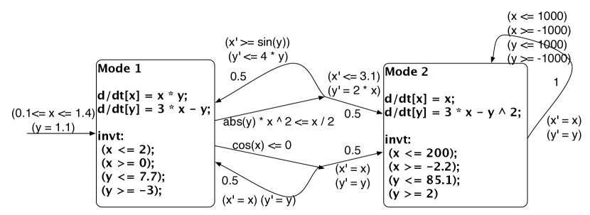
Figure 1: An example probabilistic hybrid automaton

Algorithm 1 SReach

1:function SReach($M\!P$, $ST$, $\delta$, $k$)

2:     $Succ\leftarrow 0$

3:     $N\leftarrow 0$

4:     $RV\leftarrow\mathrm{ExtractRV}(MP)$

5:     repeat

6:         $S_{i}\leftarrow\mathrm{Sim}(RV)$

7:         $M_{i}\leftarrow\mathrm{Gen}(M\!P,S_{i})$

8:         $Res\leftarrow\mathrm{dReach}(M_{i},\delta,k)$

9:         if $Res$ = $\delta$-sat then

10:              $Succ\leftarrow Succ+1$

11:         end if

12:         $N\leftarrow N+1$

13:     until $ST.done(Succ,N)$

14:   return $ST.output$

15:end function

Currently, SReach supports a number of hypothesis testing and statistical estimation techniques including: Lai’s test [26], Bayes factor test [24], Bayes factor test with indifference region [35], Sequential probability ratio test (SPRT)[34], Chernoff-Hoeffding bound [22], Bayesian Interval Estimation with Beta prior[37], and Direct Sampling. All methods produce answers which are correct up to a precision that can be set arbitrarily by the user. See Appendix A for more details about how these tests can guarantee an arbitrary small error bound between the estimated probability and the real one. With these hypothesis testing methods, SReach can answer qualitative questions, such as “Does the model satisfy a given reachability property in $k$ steps with probability greater than a certain threshold?” With the above statistical estimation techniques, SReach can offer answers to quantitative problems. For instance, “What is the probability that the model satisfies a given reachability property in $k$ steps?” SReach can also handle additional types of interesting problems by encoding them as bounded reachability problems. The model validation problem with prior knowledge can be encoded as a bounded reachability question. After expressing prior knowledge about the given model as reachability properties, is there any number of steps $k$ in which the model satisfies a given property? If none exists, the model is incorrect regarding the given prior knowledge. If, for each property, a witness is returned, we can conclude that the model is correct with regard to the prior knowledge. The parameter estimation problem can also be encoded as a $k$-step reachability problem. Does there exist a parameter combination for which the model reaches the given goal region in $k$ steps? If so, this parameter combination is potentially a good estimation for the system parameters. The goal here is to find a combination with which all the given goal regions can be reached in a bounded number of steps. Moreover, sensitivity analysis can be conducted by a set of bounded reachability queries as well: Are the results of reachability analysis the same for different possible values of a certain system parameter? If so, the model is insensitive to this parameter with regard to the given prior knowledge.

4 Experiments

Our method is implemented in the open-source tool SReach (https://github.com/dreal/SReach). Both a sequential version and a parallel one have been implemented. See Appendix C for information on using SReach. All models for the following case studies and additional benchmarks can be found on the tool website. All experiments were conducted on a server with 2* AMD Opteron(tm) Processor 6172 (24 cores) and 32GB RAM, running on Ubuntu 14.04.1 LTS. 12 cores were used. In our experiments we used $0.001$ as the precision for the $\delta$-decision problem, and Bayesian sequential estimation with $0.01$ as the estimation error bound, coverage probability $0.99$, and a uniform prior ($\alpha=\beta=1$).

Atrial Fibrillation. The minimum resistor model (MRM) reproduces experimentally measured characteristics of human ventricular cell dynamics [10]. The MRM reduces the complexity of existing models by representing channel gates of different ions with one fast channel, and two slow gates. However, due to this reduction, for most model parameters, it becomes impossible to obtain their values through measurements. After adding parametric uncertainty into the original hybrid model, we show that SReach can be adapted to estimate parameters for this stochastic model, i.e., identifying appropriate ranges and distributions for model parameters. To illustrate the way in which SReach is used to conduct parameter estimation, we chose two system parameters - $E\!P\!I\_\!T\!O1$ and $E\!P\!I\_\!T\!O2$, and varied their distributions to see which ones allow the model to present the desired pattern. The model has 4 modes. In the experiments, we chose $3$ as the unfolding depth. For each sample generated, SReach analyzed systems with $62$ variables, and $24$ ODEs. As in Table 1, when $E\!P\!I\_\!T\!O1$ is either close to $400$, or between $0.0061$ and $0.007$, and $E\!P\!I\_\!T\!O2$ is close to $6$, the model can satisfy the given bounded reachability property with a probability very close to $1$.

EPI_​T​O1	EPI_​T​O2	#S_S	#T_S	Est_P	A_T(s)	T_T(s)
U(6.1e-3, 7e-3)	6	240	240	0.996	0.270	64.80
U(5.5e-3, 5.9e-3)	6	0	240	0.004	0.042	10.08
400	U(0.131, 6)	240	240	0.996	0.231	55.36
400	U(0.1, 0.129)	0	240	0.004	0.038	9.15
N(400, 1e-4)	N(6, 1e-4)	240	240	0.996	0.091	21.87
N(5.5e-3, 10e-6)	N(0.11, 10e-5)	0	240	0.004	0.037	8.90

Table 1: Results for the atrial fibrillation model. #RVs = number of random variables in the model, #S_S = number of $\delta$-sat samples, #T_S = total number of samples, Est_P = estimated maximum posterior probability, A_T(s) = average CPU time of each sample in seconds, and T_T(s) = total CPU time for all samples in seconds.

Prostate cancer treatment. This model is a nonlinear hybrid automaton with parametric uncertainty. We modified the model of the intermittent androgen suppression (IAS) therapy in [32] by adding parametric uncertainty. The IAS therapy switches between treatment-on, and treatment-off with respect to the serum level thresholds of prostate-specific antigen (PSA), namely $r_{0}$ and $r_{1}$. As suggested by the clinical trials [9], an effective IAS therapy highly depends on the individual patient. Thus, we modified the model by taking parametric variation caused by personalized differences into account. In detail, according to clinical data from hundreds of patients [8], we replaced six system parameters with random variables having appropriate (continuous) distributions, including $\alpha_{x}$ (the proliferation rate of androgen-dependent (AD) cells), $\alpha_{y}$ (the proliferation rate of androgen-independent (AI) cells), $\beta_{x}$ (the apoptosis rate of AD cells), $\beta_{y}$ (the apoptosis rate of AI cells), $m_{1}$ (the mutation rate from AD to AI cells), and $z_{0}$ (the normal androgen level). To describe the variations due to individual differences, we assigned $\alpha_{x}$ to be $U(0.0193,0.0214)$, $\alpha_{y}$ to be $U(0.0230,0.0254)$, $\beta_{x}$ to be $U(0.0072,0.0079)$, $\beta_{y}$ to be $U(0.0160,0.0176)$, $m_{1}$ to be $U(0.0000475,0.0000525)$, and $z_{0}$ to be $N(30.0,0.001)$. We used SReach to estimate the probabilities of preventing the relapse of prostate cancer with three distinct pairs of treatment thresholds (i.e., combinations of $r_{0}$ and $r_{1}$). In the experiments, we chose $k=2$ as the unfolding depth. For each sample generated, SReach analyzed systems with $41$ variables, and $10$ ODEs. As shown in Table 2, the model with thresholds $r_{0}=10$ and $r_{1}=15$ has a maximum posterior probability that approaches 1, indicating that these thresholds may be considered for the general treatment.

$(r_{0},r_{1})$	Est_P	#S_S	#T_S	Avg_T(s)	Tot_T(s)
(5, 10)	0.496	8226	16584	0.596	9892
(7, 11)	0.994	335	336	54.307	18247
(10, 15)	0.996	240	240	506.5	121560

Table 2: Results for the prostate cancer treatment model. #S_S = number of $\delta$-sat samples, #T_S = total number of samples, $r_{0}$ = lower threshold of the serum PSA level, $r_{1}$ = upper threshold, Est_P = estimated maximum posterior probability, Avg_T(s) = average CPU time of each sample in seconds, and Tot_T(s) = total CPU time for all samples in seconds.

Synthesized Killerred Model. Due to the widespread misuse and overuse of antibiotics, drug resistant bacteria now pose significant risks to health, agriculture and the environment. An alternative to conventional antibiotics is phage-based therapy. Our approach to antibiotic resistance is to engineer a temperate phage, Lambda ($\lambda$), with light-activated production of superoxide (SOX). We incorporated the Killerred protein which has been shown to be phototoxic, and can provide another level of controlled bacteria killing [28]. A probabilistic hybrid automaton for this synthesized Killerred model, as shown in Figure 2 in Appendix D, has been constructed. Considering individual differences of bacterial cells and distinct experimental environments, additional randomness on transition probabilities were considered. SReach was first used to validate this model by estimating the probabilities of killing bacterial cells with different values for $k$, as shown in Table 3. We noticed that the probabilities of paths going through mode $6$ to mode $11$ in Figure 2 are close to $0$. To exclude the effect from sampling of rare events, we increased the probability of entering mode $6$. After this modification, the corresponding probabilities estimated by SReach still approach $0$. We conclude that it is impossible for this model to enter mode $6$. SReach was also used to (a) find out the relation between the time to turn on the light after adding the molecular biology reagent IPTG and the total time to kill bacterial cells (see Table 5 in Appendix E), (b) figure out that the lower bound for the duration of exposure to light is $3$ (see Table 6 in Appendix E), (c) find that the time to remove IPTG is not sensitive considering whether bacterial cells will be killed, and (d) estimate that the upper bound of $SOX_{thres}$ (the necessary concentration of SOX to kill bacterial cells) is $0.6667$. All these findings have been reported to biologists for further checking.

$k$	Est_P	#S_S	#T_S	Avg_T(s)	Tot_T(s)
5	0.544	8951	16452	0.074	1219.38
6	0.247	3045	12336	0.969	11957.12
7	0.096	559	5808	5.470	31770.36
8	0.004	0	240	0.004	0.88
9	0.004	0	240	0.012	2.97
10	0.004	0	240	0.013	3.18

Table 3: Results for the killerred model. #S_S = number of $\delta$-sat samples, #T_S = total number of samples, $r_{0}$ = lower threshold of the serum PSA level, $r_{1}$ = upper threshold, Est_P = estimated maximum posterior probability, Avg_T(s) = average CPU time of each sample in seconds, and Tot_T(s) = total CPU time for all samples in seconds.

Additional benchmarks. To further demonstrate the feasibility of SReach, we also applied it to additional benchmarks including hybrid systems with parametric uncertainty, PHAs, and PHAs with additional randomness. Appendix E shows the results of these experiments. Moreover, the detailed description of some of the additional benchmarks and above case studies are presented in Appendix D.

5 Conclusions and future work

We have presented a probabilistic bounded reachability analysis tool that combines $\delta$-decision procedures and statistical tests. It supports reachability analysis for hybrid systems with parametric uncertainty and probabilistic hybrid automata with additional randomness. It takes the full nondeterminism of models into account, and ensures the estimation accuracy by placing arbitrary small error bounds. This tool has been used for the probabilistic bounded reachability analysis of three representative examples - a prostate cancer treatment model, a cardiac model, and a synthesized Killerred model - which are currently out of the reach of other formal tools. In the near future, we plan to extend support for more general stochastic hybrid models that include probabilistic jumps with continuous distributions, and stochastic differential equations.

Appendix A Statistical tests

In this section we briefly describe the statistical techniques implemented in SReach. To deal with qualitative questions, SReach supports the following hypothesis testing methods.

Lai’s test [26]. As a simple class of sequential tests, it tests the one-sided composite hypotheses $H_{0}:\;\theta\leq\theta_{0}$ versus $H_{1}:\;\theta\geq\theta_{1}$ for the natural parameter $\theta$ of an exponential family of distributions under the $0-1$ loss and cost $c$ per observation. [26] shows that these tests have nearly optimal frequentist properties and also provide approximate Bayes solutions with respect to a large class of priors.

Bayes factor test [24]. The use of Bayes factors is a Bayesian alternative to classical hypothesis testing. It is based on the Bayes theorem. Hypothesis testing with Bayes factors is more robust than frequentist hypothesis testing, as the Bayesian form avoids model selection bias, evaluates evidence in favor of the null hypothesis, includes model uncertainty, and allows non-nested models to be compared. Also, frequentist significance tests become biased in favor of rejecting the null hypothesis with sufficiently large sample size.

Bayes factor test with indifference region. A hypothesis test has ideal performance if the probability of the Type-I error (respectively, Type-II error) is exactly $\alpha$ (respectively, $\beta$). However, these requirements make it impossible to ensure a low probability for both types of errors simultaneously (see [35] for details). A solution is to use an indifference region. The indifference region indicates the distance between two hypotheses, which is set to separate the two hypotheses.

Sequential probability ratio test (SPRT) [34]. The SPRT considers a simple hypothesis $H_{0}:\;\theta=\theta_{0}$ against a simple alternative $H_{1}:\;\theta=\theta_{1}$. With the critical region $\Lambda_{n}$ and two thresholds $A$, and $B$, SPRT decides that $H_{0}$ is true and stops when $\Lambda_{n}<A$. It decides that $H_{1}$ is true and terminates if $\Lambda_{n}>B$. If $A\;<\Lambda_{n}<B$, it will collect another observation to obtain a new critical region $\Lambda_{n+1}$. The SPRT is optimal, among all sequential tests, in the sense that it minimizes the average sample size.

To offer quantitative answers, SReach also supports estimation procedures as below.

Chernoff-Hoeffding bound [22]. To estimate the mean $p$ of a (bounded) random variable, given a precision $\delta^{\prime}$ and coverage probability $\alpha$, the Chernoff-Hoeffding bound computes a value $p^{\prime}$ such that $|p^{\prime}\;-\;p|\leq\delta^{\prime}$ with probability at least $\alpha$.

Bayesian Interval Estimation with Beta prior [37]. This method estimates $p$, the unknown probability that a random sampled model satisfies a specified reachability property. The estimate will be in the form of a confidence interval, containing $p$ with an arbitrary high probability. [37] assumes that the unknown $p$ is given by a random variable, whose density is called the prior density, and focuses on Beta priors.

Direct sampling. Given $N$ as the number of samples to be sampled, the direct sampling method estimates the mean of $p$ of a (bounded) random variable. According to the central limit thoerem [14], the error $\epsilon$ with a confidence $c$ between the real probability $p$ and the estimated $\hat{p}$ is bounded:
$\epsilon=\phi^{-1}\left(\frac{c+1}{2}\right)\sqrt{\frac{p(1-p)}{N}}$
where $\phi(x)=\frac{1}{\sqrt{2\pi}}\int_{-x}^{x}e^{-t^{2}/2}dt$. That is, as $N$ goes to $\infty$, the estimated probability approaches to the real one.

Appendix B $\delta$-Decisions for Hybrid Models

The reachability problems of hybrid automata can be encoded using a first-order language $\mathcal{L}_{\mathbb{R}_{\mathcal{F}}}$ over the reals, which allows the use of a wide range of real functions including nonlinear ODEs. Then, $\delta$-complete decision procedures are used to find solutions to these formulas to synthesize parameters.

Definition B.1 ($\mathcal{L}_{\mathbb{R}_{\mathcal{F}}}$-Formulas).

Let $\mathcal{F}$ be a collection of computable real functions. We define:

$$t :=x\;|\;f(t(\vec{x})),\mbox{ where }f\in\mathcal{F}\mbox{ (constants are 0-ary functions)};$$

$$\varphi :=t(\vec{x})>0\;|\;t(\vec{x})\geq 0\;|\;\varphi\wedge\varphi\;|\;\varphi\vee\varphi\;|\;\exists x_{i}\varphi\;|\;\forall x_{i}\varphi.$$

By computable real function we mean Type 2 computable, which informally requires that a (real) function can be algorithmically evaluated with arbitrary accuracy. Since in general $\mathcal{L}_{\mathbb{R}_{\mathcal{F}}}$ formulas are undecidable, the decision problem needs to be relaxed. In particular, for any $\mathcal{L}_{\mathbb{R}_{\mathcal{F}}}$ formula $\phi$ and any rational $\delta>0$ one can obtain a $\delta$-weakening formula $\phi^{\delta}$ from $\phi$ by substituting the atoms $t>0$ with $t>-\delta$ (and similarly for $t\geq 0$). Obviously, $\phi$ implies $\phi^{\delta}$, but not the vice versa. Now, the $\delta$-decision problem is deciding correctly whether:

• $\phi$ is false ($\mathsf{unsat}$);

• $\phi^{\delta}$ is true ($\delta$-$\mathsf{sat}$).

If both cases are true, then either decision is correct. More details on algorithms ($\delta$-complete decision procedures) for solving $\delta$-decision problems for $\mathcal{L}_{\mathbb{R}_{\mathcal{F}}}$ and for ODEs can be found in [19, 18, 17].

Now we state the encoding for hybrid models. Hybrid automata generalize finite-state automata by permitting continuous time flow in each discrete mode. Also, in each mode an invariant must be satisfied by the flow, and mode switches are controlled by jump conditions.

Definition B.2 ($\mathcal{L}_{\mathbb{R}_{\mathcal{F}}}$-Representations of Hybrid Automata).

A hybrid
automaton in $\mathcal{L}_{\mathbb{R}_{\mathcal{F}}}$-representation is a tuple

$$H=\langle X,Q,\{{\mathsf{flow}}_{q}(\vec{x},\vec{y},t):q\in Q\},\{\mathsf{inv}_{q}(\vec{x}):q\in Q\},\\ \{\mathsf{jump}_{q\rightarrow q^{\prime}}(\vec{x},\vec{y}):q,q^{\prime}\in Q\},\{\mathsf{init}_{q}(\vec{x}):q\in Q\}\rangle$$

where $X\subseteq\mathbb{R}^{n}$ for some $n\in\mathbb{N}$, $Q=\{q_{1},...,q_{m}\}$ is a finite set of modes, and the other components are finite sets of quantifier-free $\mathcal{L}_{\mathbb{R}_{\mathcal{F}}}$-formulas.

We now show the encoding of bounded reachability, which is used for encoding the parameter synthesis problem. We want to decide whether a given hybrid system reaches a particular region of its state space after following a (bounded) number of discrete transitions, i.e., jumps. First, we need to define auxiliary formulas used for ensuring that a particular mode is picked at a certain step.

Definition B.3.

Let $Q=\{q_{1},...,q_{m}\}$ be a set of modes. For any $q\in Q$, and $i\in\mathbb{N}$, use $b_{q}^{i}$ to represent a Boolean variable. We now define

$$\mathsf{enforce}_{Q}(q,i)=b^{i}_{q}\wedge\bigwedge_{p\in Q\setminus\{q\}}\neg b^{i}_{p}$$

$$\mathsf{enforce}_{Q}(q,q^{\prime},i)=b^{i}_{q}\wedge\neg b^{i+1}_{q^{\prime}}\wedge\bigwedge_{p\in Q\setminus\{q\}}\neg b^{i}_{p}\wedge\bigwedge_{p^{\prime}\in Q\setminus\{q^{\prime}\}}\neg b^{i+1}_{p^{\prime}}$$

We omit the subscript $Q$ when the context is clear.

We can now define the following formula that checks whether a goal region of the automaton state space is reachable after exactly $k$ discrete transitions. We first state the simpler case of a hybrid system without invariants.

Definition B.4 ($k$-Step Reachability, Invariant-Free Case).

Suppose $H$ is an invariant-free hybrid automaton, $U$ a subset of its state space represented by $\mathsf{goal}$, and $M>0$.
The formula $\mathsf{Reach}_{H,U}(k,M)$ is defined as:

$$\exists^{X}\vec{x}_{0}\exists^{X}\vec{x}_{0}^{t}\cdots\exists^{X}\vec{x}_{k}\exists^{X}\vec{x}_{k}^{t}\exists^{[0,M]}t_{0}\cdots\exists^{[0,M]}t_{k}.$$

$$\bigvee_{q\in Q}\Big{(}\mathsf{init}_{q}(\vec{x}_{0})\wedge\mathsf{flow}_{q}(\vec{x}_{0},\vec{x}_{0}^{t},t_{0})\wedge\mathsf{enforce}(q,0)\Big{)}$$

$$\wedge \bigwedge_{i=0}^{k-1}\bigg{(}\bigvee_{q,q^{\prime}\in Q}\Big{(}\mathsf{jump}_{q\rightarrow q^{\prime}}(\vec{x}_{i}^{t},\vec{x}_{i+1})\wedge\mathsf{enforce}(q,q^{\prime},i)$$

$$\hskip 31.2982pt\wedge\mathsf{flow}_{q^{\prime}}(\vec{x}_{i+1},\vec{x}_{i+1}^{t},t_{i+1})\wedge\mathsf{enforce}(q^{\prime},i+1)\Big{)}\bigg{)}$$

$$\wedge \bigvee_{q\in Q}(\mathsf{goal}_{q}(\vec{x}_{k}^{t})\wedge\mathsf{enforce}(q,k))$$

where $\exists^{X}x$ is a shorthand for $\exists x\in X$.

Intuitively, the trajectories start with some initial state satisfying $\mathsf{init}_{q}(\vec{x}_{0})$ for some $q$. Then, in each step the trajectory follows $\mathsf{flow}_{q}(\vec{x}_{i},\vec{x}_{i}^{t},t)$ and makes a continuous flow from $\vec{x}_{i}$ to $\vec{x}_{i}^{t}$ after time $t$. When the automaton makes a $\mathsf{jump}$ from mode $q^{\prime}$ to $q$, it resets variables following $\mathsf{jump}_{q^{\prime}\rightarrow q}(\vec{x}_{k}^{t},\vec{x}_{k+1})$. The auxiliary $\mathsf{enforce}$ formulas ensure that picking $\mathsf{jump}_{q\rightarrow q^{\prime}}$ in the $i$-the step enforces picking $\mathsf{flow}_{q}^{\prime}$ in the $(i+1)$-th step. When the invariants are not trivial, we need to ensure that for all the time points along a continuous flow, the invariant condition holds. We need to universally quantify over time, and the encoding is as follows:

Definition B.5 ($k$-Step Reachability, Nontrivial Invariant).

Suppose $H$ contains invariants, and $U$ is a subset of the state space represented by $\mathsf{goal}$. The $\mathcal{L}_{\mathbb{R}_{\mathcal{F}}}$-formula $\mathsf{Reach}_{H,U}(k,M)$ is defined as:

$$\exists^{X}\vec{x}_{0}\exists^{X}\vec{x}_{0}^{t}\cdots\exists^{X}\vec{x}_{k}\exists^{X}\vec{x}_{k}^{t}\exists^{[0,M]}t_{0}\cdots\exists^{[0,M]}t_{k}.$$

$$\bigvee_{q\in Q}\Big{(}\mathsf{init}_{q}(\vec{x}_{0})\wedge\mathsf{flow}_{q}(\vec{x}_{0},\vec{x}_{0}^{t},t_{0})\wedge\mathsf{enforce}(q,0)$$

$$\hskip 31.2982pt\wedge\forall^{[0,t_{0}]}t\forall^{X}\vec{x}\;(\mathsf{flow}_{q}(\vec{x}_{0},\vec{x},t)\rightarrow\mathsf{inv}_{q}(\vec{x}))\Big{)}$$

$$\wedge \bigwedge_{i=0}^{k-1}\bigg{(}\bigvee_{q,q^{\prime}\in Q}\Big{(}\mathsf{jump}_{q\rightarrow q^{\prime}}(\vec{x}_{i}^{t},\vec{x}_{i+1})\wedge\mathsf{flow}_{q^{\prime}}(\vec{x}_{i+1},\vec{x}_{i+1}^{t},t_{i+1})$$

$$\hskip 31.2982pt\wedge\mathsf{enforce}(q,q^{\prime},i)\wedge\mathsf{enforce}(q^{\prime},i+1)$$

$$\hskip 31.2982pt\wedge\forall^{[0,t_{i+1}]}t\forall^{X}\vec{x}\;(\mathsf{flow}_{q^{\prime}}(\vec{x}_{i+1},\vec{x},t)\rightarrow\mathsf{inv}_{q^{\prime}}(\vec{x})))\Big{)}\bigg{)}$$

$$\wedge \bigvee_{q\in Q}(\mathsf{goal}_{q}(\vec{x}_{k}^{t})\wedge\mathsf{enforce}(q,k)).$$

The extra universal quantifier for each continuous flow expresses the requirement that for all the time points between the initial and ending time point ($t\in[0,t_{i}+1]$) in a flow, the continuous variables $\vec{x}$ must take values that satisfy the invariant conditions $\mathsf{inv}_{q}(\vec{x})$.

Appendix C The SReach tool

C.1 Input format

The inputs to our SReach tool are descriptions of (probabilistic) hybrid automata with random variables (representing the probabilistic system parameters, and probabilistic jumps), and the reachability property to be checked. Following roughly the same format as the above definition of (probabilistic) hybrid automata, and adding the declarations of random variables, the description of an automaton is as follows.

Preprocessor. We can use the C language syntax to define constants and macros.

Variable declaration. For a random variable, the declaration specifies its distribution and name. Variables which are not random variables are required to be declared within bounds.

(Probabilistic) Hybrid automaton. A (probabilistic) hybrid automaton is represented by a set of modes. Within each mode declaration, we can specify statements for the mode invariant(s), flow function(s), and (probabilistic) jump condition(s). For a mode invariant, we can give any logic formula of the variables. A flow function is expressed by an ODE. As for a nonprobabilistic jump condition, it is written as

<logic_formula1>  ==>
            @<target_mode>  <logic_formula2>,

where the first logic formula is given as the guard of the jump, and the second one specifies the reset condition after the jump. While for a probabilistic jump condition, we need an extra constraint to express the stochastic choice, which is of the following form

(and <logic_formula1> <stochastic choice>)  ==>
            @<target_mode>  <logic_formula2>,

where the stochastic choice is a formula indicating which probabilistic transition will be chosen for this jump.

Initial conditions and Goals. Following the declaration of modes, we can declare one initial mode with corresponding conditions, and the reachability properties in the end.

Example 1. The following is an example input file for a hybrid automaton with parametric uncertainty. Currently, users can specify random variables (representing certain system parameters) with Bernoulli distribution (B), Uniform distribution (U), Gaussian distribution (N), Exponential distribution (E), and general Discrete distribution with given possible values and corresponding probabilities (DD).

⬇

1#define pi 3.1416

2N(1,0.1) mu1;

3U(10,15) thro;

4E(0.49) theta1;

5B(0.75) xinit;

6DD(0:0.7, 1:0.3) mu2;

7[0,5] x;

8[0,3] time;

9{ mode 1;

10 invt:

11 (x<=1.5);

12 (x>=0);

13 flow:

14 d/dt[x]=thro*(1/(theta1*sqrt(2*pi)))

15 *exp(0-((x-mu1+mu2)^2)/(2*theta1^2));

16 jump:

17 (x>=(thre1+5))==>@2(x’=x);

18}

19init:

20@1 (x=xinit);

21goal:

22@4 (x>=50);

Example 2. This example demonstrates the format of the input file for a probabilistic hybrid automaton with additional randomness for transition probabilities. Note that, unlike the notations of declarations of random variables representing system parameters and probabilistic transitions, declarations of random variables used to express the addtional randomness for jump probabilities start with a prefix $j$.

⬇

1jU(0.7, 0.9) pjumprv;

2DD(1:pjumprv, 2:(1 - pjumprv)) pjump1;

3DD(1:0.3, 2:0.7) pjump2;

4[-1000, 1000] x;

5[-1000, 1000] y;

6[0, 3] time;

7

8{ mode 1;

9

10 invt:

11 (x <= 2);

12 (x >= 0);

13 (y <= 7.7);

14 (y >= -3);

15 flow:

16 d/dt[x] = x * y;

17 d/dt[y] = 3 * x - y;

18 jump:

19 (and (abs(y) * x ^ 2 <= x / 2) (pjump1 = 1)) ==> @1 (and (x’ >= sin(y)) (y’ <= 4 * y));

20 (and (abs(y) * x ^ 2 <= x / 2) (pjump1 = 2)) ==> @2 (and (x’ <= 3.1) (y’ = 2 * x));

21 (and (cos(x) <= 0) (pjump2 = 1)) ==> @2 (and (x’ = x) (y’ = y));

22 (and (cos(x) <= 0) (pjump2 = 2)) ==> @1 (and (x’ = x) (y’ = y));

23}

24

25{

26 mode 2;

27 invt:

28 (x <= 200);

29 (x >= -2.2);

30 (y <= 85.1);

31 (y >= 2);

32 flow:

33 d/dt[x] = x;

34 d/dt[y] = 3 * x - y ^ 2;

35 jump:

36 (and (x <= 1000) (x >= -1000) (y <= 1000) (y >= -1000)) ==> @2 (and (x’ = x) (y’ = y));

37}

38init:

39@1 (and (x >= 0.1) (x <= 1.4) (y = 1.1));

40

41goal:

42@2 (and (x >= -10) (y >= -10));

C.2 Command line

SReach offers two choices. It can be run sequentially by typing

sreach_sq <statistical_testing_option> <filename>
¯¯<dReach> <k> <delta>,

or in parallel by

sreach_para <statistical_testing_option> <filename>
¯¯<dReach> <k> <delta>,

where:

• statistical_testing_option is a text file containing a sequence of test specifications. We will introduce the usages of statistical testing options in the following part;

• filename is a .pdrh file describing the model of a hybrid system with probabilistic system parameters. It is of the input format described in last sub-section;

• dReach is a tool for bounded reachability analysis of hybrid systems based on dReal;

• k is the number of steps of the model that the tool will explore; and

• delta is the precision for the $\delta$-decision problem.

C.3 Statistical testing options

SReach can be used with different statistical testing methods through the following specifications.

Lai’s test: Lai <theta> <cost_per_sample>, where theta indicates the probability threshold.

Bayes factor test: BFT <theta> <T> <alpha> <beta>, where theta is a probability threshold satisfying 0 < theta < 1, T is a ratio threshold satisfying T > 1, and alpha, and beta are beta prior parameters.

BFT with indifference region:
BFTI <theta> <T> <alpha> <beta> <delta>, where, besides the parameters used in the above Bayes factor test, delta is given to create the indifference region - [$p_{0}$, $p_{1}$], where $p_{0}$ = theta - delta and $p_{1}$ = theta + delta. Now, it tests $H_{0}:\;p\geq p_{0}$ against $H_{1}:\;p\leq p_{1}$ .

Sequential probability ratio test (SPRT):
SPRT <theta> <T> <delta>.

Chernoff-Hoeffding bound:
CHB <delta1> <coverage_probability>, where delta1 is the given precision, and coverage_probability indicates the confidence.

Bayesian Interval Estimation with Beta prior:
BEST <delta1> <coverage_probability> <alpha> <beta>.

Direct/Naïve Sampling: NSAM <num_of_samples>.

Appendix D Model description

Atrial Fibrillation. The model has four discrete control locations, four state variables, and nonlinear ODEs. A typical set of ODEs in the model is:

$$\frac{du}{dt} = e+(u-\theta_{v})(u_{u}-u)vg_{fi}+wsg_{si}-g_{so}(u)$$

$$\frac{ds}{dt} = \displaystyle\frac{g_{s2}}{(1+\exp(-2k(u-us)))}-g_{s2}s$$

$$\frac{dv}{dt} = -g_{v}^{+}\cdot v\hskip 28.45274pt\frac{dw}{dt}=-g_{w}^{+}\cdot w$$

The exponential term on the right-hand side of the ODE is the sigmoid function, which often appears in modelling biological switches.

Electronic Oscillator. The 3dOsc model represents an electronic oscillator model that contains nonlinear ODEs such as the following.

$$\frac{dx}{dt} = -ax\cdot sin(\omega_{1}\cdot\tau)$$

$$\frac{dy}{dt} = -ay\cdot sin((\omega_{1}+c_{1})\cdot\tau)\cdot sin(\omega_{2})\cdot 2$$

$$\frac{dz}{dt} = -az\cdot sin((\omega_{2}+c_{2})\cdot\tau)\cdot cos(\omega_{1})\cdot 2$$

$$\frac{\omega_{1}}{dt} = -c_{3}\cdot\omega_{1}\ \ \ \frac{\omega_{2}}{dt}=-c_{4}\cdot\omega_{2}\ \ \ \frac{d\tau}{dt}=1$$

Quadcopter Control. We developed a model that contains the full dynamics of a quadcopter. We use the model to solve control problems by answering reachability questions. A typical set of the differential equations are the following.

$$\frac{\mathrm{d}\omega_{x}}{\mathrm{d}t} = L\cdot k\cdot(\omega_{1}^{2}-\omega_{3}^{2})(1/I_{xx})-(I_{yy}-I_{zz})\omega_{y}\omega_{z}/I_{xx}$$

$$\frac{\mathrm{d}\omega_{y}}{\mathrm{d}t} = L\cdot k\cdot(\omega_{2}^{2}-\omega_{4}^{2})(1/I_{yy})-(I_{zz}-I_{xx})\omega_{x}\omega_{z}/I_{yy}$$

$$\frac{\mathrm{d}\omega_{z}}{\mathrm{d}t} = b\cdot(\omega_{1}^{2}-\omega_{2}^{2}+\omega_{3}^{2}-\omega_{4}^{2})(1/I_{zz})-(I_{xx}-I_{yy})\omega_{x}\omega_{y}/I_{zz}$$

$$\frac{\mathrm{d}\phi}{\mathrm{d}t} = \omega_{x}+\displaystyle{\frac{\sin\left(\phi\right)\sin\left(\theta\right)}{{\left(\frac{\sin\left(\phi\right)^{2}\cos\left(\theta\right)}{\cos\left(\phi\right)}+\cos\left(\phi\right)\cos\left(\theta\right)\right)}\cos\left(\phi\right)}}\omega_{y}$$

$$+\displaystyle\frac{\sin\left(\theta\right)}{\frac{\sin\left(\phi\right)^{2}\cos\left(\theta\right)}{\cos\left(\phi\right)}+\cos\left(\phi\right)\cos\left(\theta\right)}\omega_{z}$$

$$\frac{\mathrm{d}\theta}{\mathrm{d}t} = -(\displaystyle\frac{\sin\left(\phi\right)^{2}\cos\left(\theta\right)}{{\left(\frac{\sin\left(\phi\right)^{2}\cos\left(\theta\right)}{\cos\left(\phi\right)}\omega_{y}+\cos\left(\phi\right)\cos\left(\theta\right)\right)}\cos\left(\phi\right)^{2}}$$

$$+\frac{1}{\cos\left(\phi\right)})\omega_{y}-\displaystyle\frac{\sin\left(\phi\right)\cos\left(\theta\right)}{{\left(\frac{\sin\left(\phi\right)^{2}\cos\left(\theta\right)}{\cos\left(\phi\right)}+\cos\left(\phi\right)\cos\left(\theta\right)\right)}\cos\left(\phi\right)}\omega_{z}$$

$$\frac{\mathrm{d}\psi}{\mathrm{d}t} = \displaystyle\frac{\sin\left(\phi\right)}{{\left(\frac{\sin\left(\phi\right)^{2}\cos\left(\theta\right)}{\cos\left(\phi\right)}+\cos\left(\phi\right)\cos\left(\theta\right)\right)}\cos\left(\phi\right)}\omega_{y}$$

$$+\displaystyle\frac{1}{\frac{\sin\left(\phi\right)^{2}\cos\left(\theta\right)}{\cos\left(\phi\right)}+\cos\left(\phi\right)\cos\left(\theta\right)}\omega_{z}$$

$$\frac{\mathrm{d}{xp}}{\mathrm{d}t} = (1/m)(\sin(\theta)\sin(\psi)k(\omega_{1}^{2}+\omega_{2}^{2}+\omega_{3}^{2}+\omega_{4}^{2})-k\cdot d\cdot{xp})$$

$$\frac{\mathrm{d}{yp}}{\mathrm{d}t} = (1/m)(-\cos(\psi)\sin(\theta)k(\omega_{1}^{2}+\omega_{2}^{2}+\omega_{3}^{2}+\omega_{4}^{2})-k\cdot d\cdot{yp})$$

$$\frac{\mathrm{d}{zp}}{\mathrm{d}t} = (1/m)(-g-\cos(\theta)k(\omega_{1}^{2}+\omega_{2}^{2}+\omega_{3}^{2}+\omega_{4}^{2})-k\cdot d\cdot{zp}$$

$$\frac{\mathrm{d}x}{\mathrm{d}t} = {xp},\frac{\mathrm{d}y}{\mathrm{d}t}={yp},\frac{\mathrm{d}z}{\mathrm{d}t}={zp}$$

Prostate Cancer Treatment. The Prostate Cancer Treatment model exhibits more nonlinear ODEs.

$$\frac{dx}{dt} = (\alpha_{x}(k_{1}+(1-k_{1})\frac{z}{z+k_{2}}-\beta_{x}((1-k_{3})\frac{z}{z+k_{4}}+k_{3}))$$

$$-m_{1}(1-\frac{z}{z_{0}}))x+c_{1}x$$

$$\frac{dy}{dt} = m_{1}(1-\frac{z}{z_{0}})x+(\alpha_{y}(1-d\frac{z}{z_{0}})-\beta_{y})y+c_{2}y$$

$$\frac{dz}{dt} = \frac{-z}{\tau}+c_{3}z$$

$$\frac{dv}{dt} = (\alpha_{x}(k_{1}+(1-k_{1})\frac{z}{z+k_{2}}-\beta_{x}(k_{3}+(1-k_{3})\frac{z}{z+k_{4}}))$$

$$-m_{1}(1-\frac{z}{z_{0}}))x+c_{1}x+m_{1}(1-\frac{z}{z_{0}})x+(\alpha_{y}(1-d\frac{z}{z_{0}})$$

$$-\beta_{y})y+c_{2}y$$

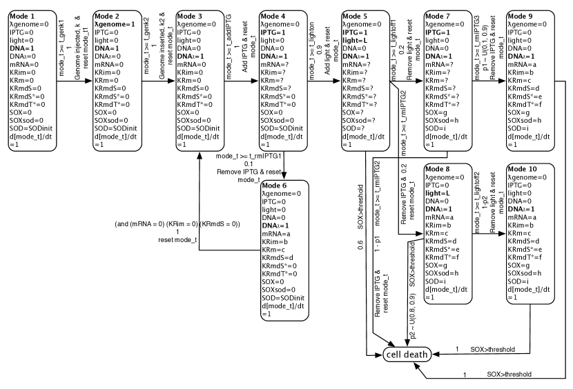
Figure 2: A probabilistic hybrid automaton for synthesized phage-based therapy model

Synthesized Killerred Model. The ODEs missing in Figure 2 are as follows.

$$\frac{\mathrm{d}[mRNA]}{\mathrm{d}t} = k_{RNAsyn}\cdot[DNA]-k_{RNAdeg}\cdot[mRNA]$$

$$\frac{\mathrm{d}[KR_{im}]}{\mathrm{d}t} = k_{KR_{im}syn}\cdot[mRNA]-(k_{KR_{m}}+k_{KR_{im}deg})$$

$$\cdot[KR_{im}]$$

$$\frac{\mathrm{d}[KR_{mdS}]}{\mathrm{d}t} = k_{KR_{m}}\cdot[KR_{im}]-k_{KR_{mdS}deg}\cdot[KR_{mdS}]$$

$$(before\;turning\;on\;the\;light)$$

$$\frac{\mathrm{d}[KR_{mdS}]}{\mathrm{d}t} = k_{KR_{m}}\cdot[KR_{im}]+k_{KR_{f}}\cdot[KR_{mdS^{*}}]$$

$$+k_{KR_{ic}}\cdot[KR_{mdS^{*}}]+k_{KR_{nrd}}\cdot[KR_{mdT^{*}}]$$

$$+k_{KR_{SOXd1}}\cdot[KR_{mdT^{*}}]-k_{KR_{ex}}\cdot[KR_{mdS}]$$

$$-k_{KR_{mdS}deg}\cdot[KR_{mdS}]\;\;\;(after\;adding\;light)$$

$$\frac{\mathrm{d}[KR_{mdS^{*}}]}{\mathrm{d}t} = k_{KR_{ex}}\cdot[KR_{mdS}]-k_{KR_{f}}\cdot[KR_{mdS^{*}}]$$

$$-k_{KR_{ic}}\cdot[KR_{mdS^{*}}]-k_{KR_{isc}}\cdot[KR_{mdS^{*}}]$$

$$-k_{KR_{mdS^{*}}deg}\cdot[KR_{mdS^{*}}]$$

$$\frac{\mathrm{d}[KR_{mdT^{*}}]}{\mathrm{d}t} = k_{KR_{isc}}\cdot[KR_{mdS^{*}}]-k_{KR_{nrd}}\cdot[KR_{mdT^{*}}]$$

$$-k_{KR_{SOXd1}}\cdot[KR_{mdT^{*}}]$$

$$-k_{KR_{SOXd2}}\cdot[KR_{mdT^{*}}]$$

$$-k_{KR_{mdT^{*}}deg}\cdot[KR_{mdT^{*}}]$$

$$\frac{\mathrm{d}[SOX]}{\mathrm{d}t} = k_{KR_{SOXd1}}\cdot[KR_{mdT^{*}}]+k_{KR_{SOXd2}}\cdot[KR_{mdT^{*}}]$$

$$-\frac{\mathrm{d}[SOX_{sod}]}{\mathrm{d}t}$$

$$\frac{\mathrm{d}[SOX_{sod}]}{\mathrm{d}t} = k_{SOD}\cdot V_{maxSOD}\cdot\frac{[SOX]}{K_{m}+[SOX]}$$

Appendix E Experimental results for additional benchmarks

Benchmark	#Ms	K	#ODEs	#Vs	#RVs	$\delta$	Est_P	#S_S	#T_S	A_T(s)	T_T(s)
BBK1	1	1	2	14	3	0.001	0.754	5372	7126	0.086	612.836
BBK5	1	5	2	38	3	0.001	0.059	209	3628	0.253	917.884
BBwDv1	2	2	4	20	4	0.001	0.208	2206	10919	0.080	873.522
BBwDv2K2	2	2	4	20	3	0.001	0.845	7330	8669	0.209	1811.821
BBwDv2K8	2	8	4	56	3	0.001	0.207	2259	10901	0.858	9353.058
Tld	2	7	2	33	4	0.001	0.996	227	227	0.213	48.351
Ted	2	7	4	50	4	0.001	0.996	227	227	12.839	2914.448
DTldK3	2	3	4	26	2	0.001	0.996	227	227	0.382	86.714
DTldK5	2	5	4	38	2	0.001	0.161	1442	8961	0.280	2509.078
W4mv1	4	3	8	26	6	0.001	0.381	5953	15639	0.238	3722.082
W4mv2K3	4	3	8	26	6	0.001	0.996	227	227	0.673	152.771
W4mv2K7	4	7	8	50	6	0.001	0.004	0	227	0.120	27.240
DWK1	2	1	4	14	5	0.001	0.996	227	227	0.171	38.817
DWK3	2	3	4	26	5	0.001	0.996	227	227	0.215	48.806
DWK9	2	9	4	62	5	0.001	0.996	227	227	5.144	1167.688
Que	3	2	3	13	4	0.001	0.228	2662	11677	0.095	1109.315
3dOsc	3	2	18	48	2	0.001	0.996	227	227	8.273	1877.969
QuadC	1	0	14	44	6	0.001	0.996	227	227	825.641	187420.507
ExPHA01	2	2	4	20	2	0.001	0.524	345	658	5.01	3295.82
ExPHA02	2	3	2	17	1	0.001	0.900	5361	5953	0.0004	2.35
KRk5	6	5	84	194	2	0.001	0.544	8946	16457	0.122	2015.64
KRk6	8	6	112	224	6	0.001	0.246	2032	8263	1.385	11444.22
KRk7	10	7	150	271	6	0.001	0.096	558	5795	16.275	94311.18
KRk8	7	8	105	303	6	0.001	0.004	0	227	0.003	0.58
KRk9	9	9	135	335	6	0.001	0.004	0	227	0.015	3.43
KRk10	11	10	165	367	6	0.001	0.004	0	227	0.026	5.92

Table 4: #Ms = number of modes, K indicates the unfolding steps, #ODEs = number of ODEs in the model, #Vs = number of total variables in the unfolded formulae, #RVs = number of random variables in the model, $\delta$ = precision used in dReach, #S_S = number of $\delta$-sat samples , #T_S = total number of samples, Est_P = estimated maximum posterior probability, A_T(s) = average CPU time of each sample in seconds, and T_T(s) = total CPU time for all samples in seconds.

$t_{lighton}$	1	2	3	4	5	6	7	8	9	10
$t_{tot}$	16	17.2	18.5	20	21.3	22.7	23.5	24.1	25	30

Table 5: The relation between the time to turn on the light after adding IPTG and the total time to kill bacteria cells ($k=5$).

$t_{lightoff1}$	1	2	3	4	5	6	7	8	9	10
$killbacteriacells$	Failed	Failed	Failed	Succ	Succ	Succ	Succ	Succ	Succ	Succ

Table 6: The impact of the time duration that the cells are exposed to light ($k=6$).

The table 4 shows the results of experiments. To further demonstrate the feasibility of SReach, these experiments were conducted with the sequential version of SReach on a machine with 2.9GHz Intel Core i7 processor and 8GB RAM, running OS X 10.9.2. In our experiments we used $0.001$ as the precision for the $\delta$-decision problem; and Bayesian sequential estimation with $0.01$ half-interval width, coverage probability $0.99$, and uniform prior ($\alpha=\beta=1$). In the following table, BB refers to the bouncing ball models, Tld the thermostat model with linear temperature decrease, Ted the thermostat model with exponential decrease, DT the dual thermostat models, W the watertank models, DW the dual watertank models, Que the model for queuing system which has both nonlinear functions and nondeterministic jumps, 3dOsc the model for 3d oscillator, and QuadC the model for quadcopter stabilization control. Following these hybrid systems with parametric uncertainty, we also consider two example PHAs - ExPHA01and EXPHA02, and PHAs with additional randomness - KR our killerred models.

References

- [1] A. Abate. Probabilistic reachability for stochastic hybrid systems: Theory, computations, and applications. Technical Report UCB/EECS-2007-132, UC Berkeley, 2007.
- [2] A. Abate, J.-P. Katoen, J. Lygeros, and M. Prandini. A two-step scheme for approximate model checking of stochastic hybrid systems. In IFAC, 2011.
- [3] A. Abate, J.-P. Katoen, and A. Mereacre. Quantitative automata model checking of autonomous stochastic hybrid systems. In HSCC, pages 83–92. ACM, 2011.
- [4] S. Amin, A. Abate, M. Prandini, J. Lygeros, and S. Sastry. Reachability analysis for controlled discrete time stochastic hybrid systems. In HSCC, pages 49–63. Springer, 2006.
- [5] L. Arnold. Stochastic Differential Equations: Theory and Applications. Wiley - Interscience, 1974.
- [6] H. A. Blom and E. A. Bloem. Particle filtering for stochastic hybrid systems. In CDC, volume 3, pages 3221–3226. IEEE, 2004.
- [7] H. A. Blom, J. Lygeros, M. Everdij, S. Loizou, and K. Kyriakopoulos. Stochastic hybrid systems: theory and safety critical applications. Springer, 2006.
- [8] N. Bruchovsky, L. Klotz, J. Crook, and L. Goldenberg. Locally advanced prostate cancer: biochemical results from a prospective phase ii study of intermittent androgen suppression for men with evidence of prostate-specific antigen recurrence after radiotherapy. Cancer, 109(5):858–867, 2007.
- [9] N. Bruchovsky, L. Klotz, et al. Final results of the Canadian prospective phase ii trial of intermittent androgen suppression for men in biochemical recurrence after radiotherapy for locally advanced prostate cancer. Cancer, 107(2):389–395, 2006.
- [10] A. Bueno-Orovio, E. M. Cherry, and F. H. Fenton. Minimal model for human ventricular action potentials in tissue. J. of Theor. Biology, 253(3):544–560, 2008.
- [11] E. M. Clarke and P. Zuliani. Statistical model checking for cyber-physical systems. In ATVA, pages 1–12. Springer, 2011.
- [12] L. Cordeiro, B. Fischer, and J. Marques-Silva. Smt-based bounded model checking for embedded ansi-c software. Software Engineering, IEEE, 38(4):957–974, 2012.
- [13] A. David, D. Du, K. G. Larsen, A. Legay, M. Mikučionis, D. B. Poulsen, and S. Sedwards. Statistical model checking for stochastic hybrid systems. arXiv preprint arXiv:1208.3856, 2012.
- [14] R. Durrett. Probability: theory and examples. Cambridge University Press, 2010.
- [15] M. Fränzle, E. M. Hahn, H. Hermanns, N. Wolovick, and L. Zhang. Measurability and safety verification for stochastic hybrid systems. In HSCC, pages 43–52, Apr. 2011.
- [16] M. Fränzle, H. Hermanns, and T. Teige. Stochastic satisfiability modulo theory: A novel technique for the analysis of probabilistic hybrid systems. In HSCC, pages 172–186. Springer, 2008.
- [17] S. Gao, S. Kong, W. Chen, and E. M. Clarke. -complete analysis for bounded reachability of hybrid systems. CoRR, arXiv:1404.7171, 2014.
- [18] S. Gao, S. Kong, and E. M. Clarke. dReal: An SMT solver for nonlinear theories over the reals. In CADE, pages 208–214. Springer, 2013.
- [19] S. Gao, S. Kong, and E. M. Clarke. Satisfiability modulo ODEs. In FMCAD, pages 105–112, Oct. 2013.
- [20] E. M. Hahn, G. Norman, D. Parker, B. Wachter, and L. Zhang. Game-based abstraction and controller synthesis for probabilistic hybrid systems. In QEST, pages 69–78. IEEE, 2011.
- [21] T. A. Henzinger. The theory of hybrid automata. Springer, 2000.
- [22] W. Hoeffding. Probability inequalities for sums of bounded random variables. J American Statistical Association, 58(301):13–30, 1963.
- [23] J. Hu, J. Lygeros, and S. Sastry. Towards a theory of stochastic hybrid systems. In HSCC, pages 160–173. Springer, 2000.
- [24] R. E. Kass and A. E. Raftery. Bayes factors. JASA, 90(430):773–795, 1995.
- [25] M. Kwiatkowska, G. Norman, and D. Parker. PRISM 4.0: Verification of probabilistic real-time systems. In CAV, volume 6806, pages 585–591. Springer, 2011.
- [26] T. L. Lai. Nearly optimal sequential tests of composite hypotheses. AOS, 16(2):856–886, 1988.
- [27] K. G. Larsen, P. Pettersson, and W. Yi. Uppaal in a nutshell. STTT, 1(1):134–152, 1997.
- [28] N. Miskov-Zivanov, Q. Wang, C. Telmer, and E. M. Clarke. Formal analysis provides parameters for guiding hyperoxidation in bacteria using phototoxic proteins. Technical Report CMU-CS-14-137, CMU, 2014.
- [29] A. Platzer. Stochastic differential dynamic logic for stochastic hybrid programs. In CADE, pages 446–460. Springer, 2011.
- [30] J. Sproston. Decidable model checking of probabilistic hybrid automata. In FTRTFT, pages 31–45. Springer, 2000.
- [31] J. Sproston. Model checking for probabilistic timed and hybrid systems. In PhD thesis. SCS, University of Birmingham, 2001.
- [32] G. Tanaka, Y. Hirata, L. Goldenberg, N. Bruchovsky, and K. Aihara. Mathematical modelling of prostate cancer growth and its application to hormone therapy. Phil. Trans. Roy. Soc. A: Math., Phys. and Eng. Sci., 368(1930):5029–5044, 2010.
- [33] C. Tinelli. SMT-based model checking. In NASA FM, page 1, 2012.
- [34] A. Wald. Sequential tests of statistical hypotheses. The Annals of Mathematical Statistics, 16(2):117–186, 1945.
- [35] H. L. Younes. Verification and planning for stochastic processes with asynchronous events. Technical report, DTIC Document, 2005.
- [36] L. Zhang, Z. She, S. Ratschan, H. Hermanns, and E. M. Hahn. Safety verification for probabilistic hybrid systems. EJC, 18(6):572–587, 2012.
- [37] P. Zuliani, A. Platzer, and E. M. Clarke. Bayesian statistical model checking with application to stateflow/simulink verification. Formal Methods in System Design, 43(2):338–367, 2013.