Randomized Sketches of Convex Programs
with Sharp
Guarantees
| Mert Pilanci⋆ | Martin J. Wainwright⋆,† |
{mert,wainwrig}@berkeley.edu
⋆Department of Electrical Engineering and Computer Science †Department of Statistics
University of California, Berkeley
Abstract
Random projection (RP) is a classical technique for reducing storage and computational costs. We analyze RP-based approximations of convex programs, in which the original optimization problem is approximated by the solution of a lower-dimensional problem. Such dimensionality reduction is essential in computation-limited settings, since the complexity of general convex programming can be quite high (e.g., cubic for quadratic programs, and substantially higher for semidefinite programs). In addition to computational savings, random projection is also useful for reducing memory usage, and has useful properties for privacy-sensitive optimization. We prove that the approximation ratio of this procedure can be bounded in terms of the geometry of constraint set. For a broad class of random projections, including those based on various sub-Gaussian distributions as well as randomized Hadamard and Fourier transforms, the data matrix defining the cost function can be projected down to the statistical dimension of the tangent cone of the constraints at the original solution, which is often substantially smaller than the original dimension. We illustrate consequences of our theory for various cases, including unconstrained and -constrained least squares, support vector machines, low-rank matrix estimation, and discuss implications on privacy-sensitive optimization and some connections with denoising and compressed sensing.
1 Introduction
Optimizing a convex function subject to constraints is fundamental to many disciplines in engineering, applied mathematics, and statistics [7, 28]. While most convex programs can be solved in polynomial time, the computational cost can still be prohibitive when the problem dimension and/or number of constraints are large. For instance, although many quadratic programs can be solved in cubic time, this scaling may be prohibitive when the dimension is on the order of millions. This type of concern is only exacerbated for more sophisticated cone programs, such as second-order cone and semidefinite programs. Consequently, it is of great interest to develop methods for approximately solving such programs, along with rigorous bounds on the quality of the resulting approximation.
In this paper, we analyze a particular scheme for approximating a convex program defined by minimizing a quadratic objective function over an arbitrary convex set. The scheme is simple to describe and implement, as it is based on performing a random projection of the matrices and vectors defining the objective function. Since the underlying constraint set may be arbitrary, our analysis encompasses many problem classes including quadratic programs (with constrained or penalized least-squares as a particular case), as well as second-order cone programs and semidefinite programs (including low-rank matrix approximation as a particular case).
An interesting class of such optimization problems arise in the context of statistical estimation. Many such problems can be formulated as estimating an unknown parameter based on noisy linear measurements, along with side information that the true parameter belongs to a low-dimensional space. Examples of such low-dimensional structure include sparse vectors, low-rank matrices, discrete sets defined in a combinatorial manner, as well as algebraic sets, including norms for inducing shrinkage or smoothness. Convex relaxations provide a principled way of deriving polynomial-time methods for such problems [7], and their statistical performance has been extensively studied over the past decade (see the papers [8, 35] for overviews). For many such problems, the ambient dimension of the parameter is very large, and the number of samples can also be large. In these contexts, convex programs may be difficult to solve exactly, and reducing the dimension and sample size by sketching is a very attractive option.
Our work is related to a line of work on sketching unconstrained least-squares problems (e.g., see the papers [15, 22, 6] and references therein). The results given here generalizes this line of work by providing guarantees for the broader class of constrained quadratic programs. In addition, our techniques are convex-analytic in nature, and by exploiting analytical tools from Banach space geometry and empirical process theory [12, 19, 18], lead to sharper bounds on the sketch size as well as sharper probabilistic guarantees. Our work also provides a unified view of both least-squares sketching [15, 22, 6] and compressed sensing [13, 14]. As we discuss in the sequel, various results in compressed sensing can be understood as special cases of sketched least-squares, in which the data matrix in the original quadratic program is the identity.
In addition to reducing computation and storage, random projection is also useful in the context of privacy preservation. Many types of modern data, including financial records and medical tests, have associated privacy concerns. Random projection allows for a sketched version of the data set to be stored, but such that there is a vanishingly small amount of information about any given data point. Our theory shows that this is still possible, while still solving a convex program defined by the data set up to -accuracy. In this way, we sharpen some results by Zhou and Wasserman [37] on privacy-preserving random projections for sparse regression. Our theory points to an interesting dichotomy in privacy sensitive optimization problems based on the trade-off between the complexity of the constraint set and mutual information. We show that if the constraint set is simple enough in terms of a statistical measure, privacy sensitive optimization can be done with arbitrary accuracy.
The remainder of this paper is organized as follows. We begin in Section 2 with a more precise formulation of the problem, and the statement of our main results. In Section 3, we derive corollaries for a number of concrete classes of problems, and provide various simulations that demonstrate the close agreement between the theoretical predictions and behavior in practice. Sections 4 and Section 5 are devoted to the proofs our main results, and we conclude in Section 6. Parts of the results given here are to appear in the conference form at the International Symposium on Information Theory (2014).
2 Statement of main results
We begin by formulating the problem analyzed in this paper, before turning to a statement of our main results.
2.1 Problem formulation
Consider a convex program of the form
| (1) |
where is some convex subset of , and are a data vector and data matrix, respectively. Our goal is to obtain an -optimal solution to this problem in a computationally simpler manner, and we do so by projecting the problem into , where , via a sketching matrix . In particular, consider the sketched problem
| (2) |
Note that by the optimality and feasibility of and , respectively, for the original problem (1), we always have . Accordingly, we say that is an -optimal approximation to the original problem (1) if
| (3) |
Our main result characterizes the number of samples required to achieve this bound as a function of , and other problem parameters.
Our analysis involves a natural geometric object in convex analysis, namely the tangent cone of the constraint set at the optimum , given by
| (4) |
where denotes the closed convex hull. This set arises naturally in the convex optimality conditions for the original problem (1): any vector defines a feasible direction at the optimal , and optimality means that it is impossible to decrease the cost function by moving in directions belonging to the tangent cone.
We use to denote the linearly transformed cone . Our main results involve measures of the “size” of this transformed cone when it is intersected with the Euclidean sphere . In particular, we define Gaussian width of the set via
| (5) |
where is an i.i.d. sequence of variables. This complexity measure plays an important role in Banach space theory, learning theory and statistics (e.g., [31, 19, 5]).
2.2 Guarantees for sub-Gaussian sketches
Our first main result provides a relation between the sufficient sketch size and Gaussian complexity in the case of sub-Gaussian sketches. In particular, we say that a row of the sketching matrix is -sub-Gaussian if it is zero-mean, and if for any fixed unit vector , we have
| (6) |
Of course, this condition is satisfied by the standard Gaussian sketch (). In addition, it holds for various other sketching matrices, including random matrices with i.i.d. Bernoulli elements, random matrices with rows drawn uniformly from the rescaled unit sphere, and so on. We say that the sketching matrix is drawn from a -sub-Gaussian ensemble if each row is -sub-Gaussian in the previously defined sense (6).
Theorem 1 (Guarantees for sub-Gaussian projections).
Let be drawn from a -sub-Gaussian ensemble. Then there are universal constants such that, for any tolerance parameter , given a sketch size lower bounded as
| (7) |
the approximate solution is guaranteed to be -optimal (3) for the original program with probability at least .
As will be clarified in examples to follow, the squared
width scales proportionally to the
statistical dimension, or number of degrees of freedom in the set
. Consequently, up to constant factors,
Theorem 1 guarantees that we can project down to the
statistical dimension of the problem while preserving
-optimality of the solution.
This fact has an interesting corollary in the context of privacy-sensitive optimization. Suppose that we model the data matrix as being random, and our goal is to solve the original convex program (1) up to -accuracy while revealing as little as possible about the individual entries of . By Theorem 1, whenever the sketch dimension satisfies the lower bound (7), the sketched data matrix suffices to solve the original program up to -accuracy. We can thus ask about how much information per entry of is retained by the sketched data matrix. One way in which to do so is by computing the mutual information per symbol, namely
where the rescaling is chosen since has a total of entries. This quantity was studied by Zhou and Wasserman [37] in the context of privacy-sensitive sparse regression, in which is an -ball, to be discussed at more in length in Section 3.2. In our setting, we have the following more generic corollary of Theorem 1:
Corollary 1.
Let the entries of be drawn i.i.d. from a distribution with finite variance . Byusing random Gaussian projections, we can ensure that
| (8) |
and that the sketched solution is -optimal with probability at least .
Note that the inequality always holds. However, for many problems, we have the much stronger guarantee , in which case the bound (8) guarantees that the mutual information per symbol is vanishing. There are various concrete problems, as discussed in Section 3, for which this type of scaling is reasonable. Thus, for any fixed , we are guaranteed a -optimal solution with a vanishing mutual information per symbol.
Corollary 1 follows by a straightforward combination of past work [37] with Theorem 1. Zhou and Wasserman [37] show that under the stated conditions, for a standard i.i.d. Gaussian sketching matrix , the mutual information rate per symbol is upper bounded as
Substituting in the stated choice of and applying Theorem 1 yields the claim.
2.3 Guarantees for randomized orthogonal systems
A possible disadvantage of using sub-Gaussian sketches is that it requires performing matrix-vector multiplications with unstructured random matrices; such multiplications require time in general. Our second main result applies to sketches based on a randomized orthonormal system (ROS), for which matrix multiplication can be performed much more quickly.
In order to define a randomized orthonormal system, we begin by with an orthonormal matrix with entries . A standard class of such matrices is provided by the Hadamard basis, for which matrix-vector multiplication can be performed in time. Another possible choice is the Fourier basis. Based on any such matrix, a sketching matrix from a ROS ensemble is obtained by sampling i.i.d. rows of the form
where the random vector is chosen uniformly at random from the set of all canonical basis vectors, and is a diagonal matrix of i.i.d. Rademacher variables . With the base matrix chosen as the Hadamard or Fourier basis, then for any fixed vector , the product can be computed in time (e.g., see the paper [2] for details). Hence the sketched data can be formed in time, which scales almost linearly in the input size .
Our main result for randomized orthonormal systems involves the -Gaussian width of the set , given by
| (9) |
As will be clear in the corollaries to follow, in many cases, the -Gaussian width is equivalent to the ordinary Gaussian width (5) up to numerical constants. It also involves the Rademacher width of the set , given by
| (10) |
where is an i.i.d. vector of Rademacher variables.
Theorem 2 (Guarantees for randomized orthonormal system).
Let be drawn from a randomized orthonormal system (ROS). Then given a sample size lower bounded as
| (11) |
the approximate solution is guaranteed to be -optimal (3) for the original program with probability at least .
The required projection dimension (11) for ROS sketches is in general larger than that required for sub-Gaussian sketches, due to the presence of the additional pre-factor . For certain types of cones, we can use more specialized techniques to remove this pre-factor, so that it is not always required. The details of these arguments are given in Section 5, and we provide some illustrative examples of such sharpened results in the corollaries to follow. However, the potentially larger projection dimension is offset by the much lower computational complexity of forming matrix vector products using the ROS sketching matrix.
3 Some concrete instantiations
Our two main theorems are general results that apply to any choice of the convex constraint set . We now turn to some consequences of Theorems 1 and 2 for more specific classes of problems, in which the geometry enters in different ways.
3.1 Unconstrained least squares
We begin with the simplest possible choice, namely , which leads to an unconstrained least squares problem. This class of problems has been studied extensively in past work on least-square sketching [22]; our derivation here provides a sharper result in a more direct manner. At least intuitively, given the data matrix , it should be possible to reduce the dimensionality to the rank of the data matrix , while preserving the accuracy of the solution. In many cases, the quantity is substantially smaller than . The following corollaries of Theorem 1 and 2 confirm this intuition:
Corollary 2 (Approximation guarantee for unconstrained least squares).
This corollary improves known results both in the probability estimate and required samples, in particular previous results hold only with constant probability; see the paper [22] for an overview of such results. Note that the total computational complexity of computing and solving the sketched least squares problem, for instance via QR decomposition [16], is of the order for sub-Gaussian sketches, and of the order for ROS sketches. Consequently, by using ROS sketches, the overall complexity of computing a -approximate least squares solution with exponentially high probability is . In many cases, this complexity is substantially lower than direct computation of the solution via QR decomposition, which would require operations.
Proof.
Since , the tangent cone is all of , and the set is the image of . Thus, we have
| (12) |
where the inequality follows from the the fact that the image of is at most -dimensional. Thus, the sub-Gaussian bound in part (a) is an immediate consequence of Theorem 1.
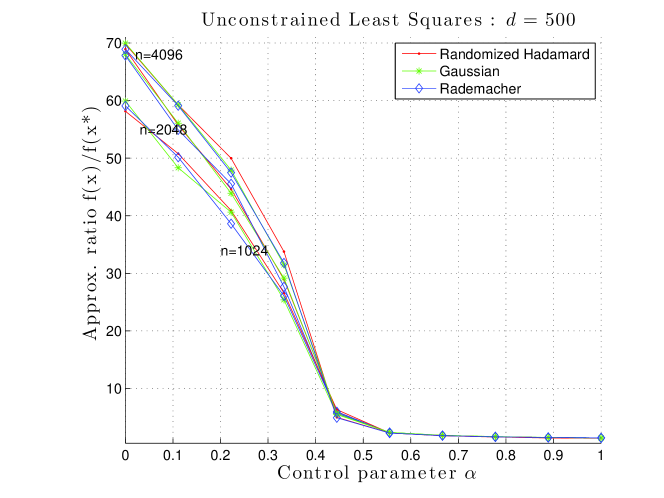
In order to investigate the theoretical prediction of Corollary 2, we performed some simple simulations on randomly generated problem instances. Fixing a dimension , we formed a random ensemble of least-squares problems by first generating a random data matrix with i.i.d. standard Gaussian entries. For a fixed random vector , we then computed the data vector , where the noise vector where . Given this random ensemble of problems, we computed the projected data matrix-vector pairs using Gaussian, Rademacher, and randomized Hadamard sketching matrices, and then solved the projected convex program. We performed this experiment for a range of different problem sizes . For any in this set, we have , with high probability over the choice of randomly sampled . Suppose that we choose a projection dimension of the form , where the control parameter ranged over the interval . Corollary 2 predicts that the approximation error should converge to under this scaling, for each choice of .
3.2 -constrained least squares
We now turn a constrained form of least-squares, in which the geometry of the tangent cone enters in a more interesting way. In particular, consider the following -constrained least squares program, known as the Lasso [9, 34]
| (13) |
It is is widely used in signal processing and statistics for sparse signal recovery and approximation.
In this section, we show that as a corollary of Theorem 1, this quadratic program can be sketched logarithmically in dimension when the optimal solution to the original problem is sparse. In particular, assuming that is unique, we let denote the number of non-zero coefficients of the unique solution to the above program. (When is not unique, we let denote the minimal cardinality among all optimal vectors). Define the -restricted eigenvalues of the given data matrix as
| (14) |
Corollary 3 (Approximation guarantees for -constrained least squares).
Consider the -constrained least squares problem (13):
We note that part (a) of this corollary improves the result of Zhou et al. [37], which establishes consistency of Lasso with a Gaussian sketch dimension of the order , in contrast to the requirement in the bound (15). To be more precise, these two results are slightly different, in that the result [37] focuses on support recovery, whereas Corollary 3 guarantees a -accurate approximation of the cost function.
Let us consider the complexity of solving the sketched problem using different methods. In the regime , the complexity of solving the original Lasso problem as a linearly constrained quadratic program via interior point solvers is per iteration (e.g., see Nesterov and Nemirovski [30]). Thus, computing the sketched data and solving the sketched Lasso problem requires operations for sub-Gaussian sketches, and for ROS sketches.
Another popular choice for solving the Lasso problem is to use a first-order algorithm [29]; such algorithms require operations per iteration, and yield a solution that is -optimal within iterations. If we apply such an algorithm to the sketched version for steps, then we obtain a vector such that
Overall, obtaining this guarantee requires operations for sub-Gaussian sketches, and operations for ROS sketches.
Proof.
Let denote the support of the optimal solution . The tangent cone to the -norm constraint at the optimum takes the form
| (17) |
where is the sign vector of the optimal solution on its support. By the triangle inequality, any vector satisfies the inequality
| (18) |
If , then by the definition (14), we also have the upper bound , whence
| (19) |
Note that is a -dimensional Gaussian vector, in which the -entry has variance . Consequently, inequality (19) combined with standard Gaussian tail bounds [19] imply that
| (20) |
Combined with the bound from Corollary 2, also applicable in this setting, the claim (15) follows.
Turning to part (b), the first lower bound involving follows from Corollary 2. The second lower bound follows as a corollary of Theorem 2 in application to the Lasso; see Appendix A for the calculations. The third lower bound follows by a specialized argument given in Section 5.3.
∎
In order to investigate the prediction of Corollary 3, we generated a random ensemble of sparse linear regression problems as follows. We first generated a data matrix by sampling i.i.d. standard Gaussian entries, and then a -sparse base vector by choosing a uniformly random subset of size , and setting its entries to in independent and equiprobably. Finally, we formed the data vector , where the noise vector has i.i.d. entries.
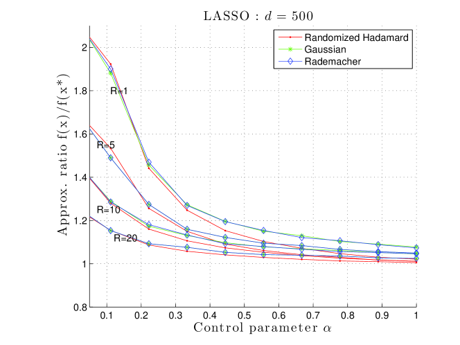
In our experiments, we solved the Lasso (13) with a choice of radius parameter , and set . We then set the projection dimension where is a control parameter, and solved the sketched Lasso for Gaussian, Rademacher and randomized Hadamard sketching matrices. Our theory predicts that the approximation ratio should tend to one as the control parameter increases. The results are plotted in Figure 2, and confirm this qualitative prediction.
3.3 Compressed sensing and noise folding
It is worth noting that various compressed sensing results can be recovered as a special case of Corollary 3—more precisely, one in which the “data matrix” is simply the identity (so that ). With this choice, the original problem (1) corresponds to the classical denoising problem, namely
| (21) |
so that the cost function is simply . With the choice of constraint set , the optimal solution to the original problem is unique, and can be obtained by performing a coordinate-wise soft-thresholding operation on the data vector . For this choice, the sketched version of the de-noising problem (21) is given by
| (22) |
Noiseless version:
In the noiseless version of compressed sensing, we have , and hence the optimal solution to the original “denoising” problem (21) is given by , with optimal value
Using the sketched data vector , we can solve the sketched program (22). If doing so yields a -approximation , then in this special case, we are guaranteed that
| (23) |
which implies that we have exact recovery—that is, .
Noisy versions:
In a more general setting, we observe the vector , where and is some type of observation noise. The sketched observation model then takes the form
so that the sketching matrix is applied to both the true vector and the noise vector . This set-up corresponds to an instance of compressed sensing with “folded” noise (e.g., see the papers [3, 1]), which some argue is a more realistic set-up for compressed sensing. In this context, our results imply that the sketched version satisfies the bound
| (24) |
If we think of as an approximately sparse vector and as
the best approximation to from the -ball, then this
bound (24) guarantees that we recover a
-approximation to the best sparse approximation. Moreover,
this bound shows that the compressed sensing error should be closely
related to the error in denoising, as has been made precise in recent
work [14].
Let us summarize these conclusions in a corollary:
Corollary 4.
Consider an instance of the denoising problem (21) when .
- (a)
-
(b)
For ROS sketches, the same conclusions hold with probability using a sketch dimension
(25)
Of course, a more general version of this corollary holds for any convex constraint set , involving the Gaussian/Rademacher width functions. In this more setting, the corollary generalizes results by Chandrasekaran et al. [8], who studied randomized Gaussian sketches in application to atomic norms, to other types of sketching matrices and other types of constraints. They provide a number of calculations of widths for various atomic norm constraint sets, including permutation and orthogonal matrices, and cut polytopes, which can be used in conjunction with the more general form of Corollary 4.
3.4 Support vector machine classification
Our theory also has applications to learning linear classifiers based on labeled samples. In the context of binary classification, a labeled sample is a pair , where the vector represents a collection of features, and is the associated class label. A linear classifier is specified by a function , where is a weight vector to be estimated.
Given a set of labelled patterns , the support vector machine [10, 33] estimates the weight vector by minimizing the function
| (26) |
In this formulation, the squared hinge loss is used to measure the performance of the classifier on sample , and the quadratic penalty serves as a form of regularization.
By considering the dual of this problem, we arrive at a least-squares problem that is amenable to our sketching techniques. Let be a matrix with as its column, and let be a diagonal matrix and let . With this notation, the associated dual problem (e.g. see the paper [20]) takes the form
| (27) |
The optimal solution corresponds to a vector of weights associated with the samples: it specifies the optimal SVM weight vector via . It is often the case that the dual solution has relatively few non-zero coefficients, corresponding to samples that lie on the so-called margin of the support vector machine.
The sketched version is then given by
| (28) |
The simplex constraint in the quadratic program (27), although not identical to an -constraint, leads to similar scaling in terms of the sketch dimension.
Corollary 5 (Sketch dimensions for support vector machines).
We omit the proof, as the calculations specializing from
Theorem 1 are essentially the same as those of
Corollary 3. The computational complexity of solving the SVM problem as a linearly constrained quadratic problem is same with the Lasso problem, hence same conclusions apply.
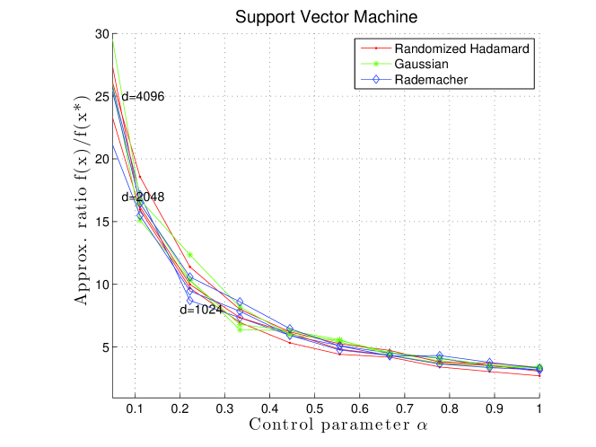
In order to study the prediction of Corollary 5, we generated some classification experiments, and tested the performance of the sketching procedure. Consider a two-component Gaussian mixture model, based on the component distributions and , where and are uniformly distributed in . Placing equal weights on each component, we draw samples from this mixture distribution, and then use the resulting data to solve the SVN dual program (27), thereby obtaining an optimal linear decision boundary specified by the vector . The number of non-zero entries corresponds to the number of examples on the decision boundary, known as support vectors. We then solve the sketched version (28), using either Gaussian, Rademacher or randomized Hadamard sketches, and using a projection dimension scaling as , where is a control parameter. We repeat this experiment for problem dimensions , performing trials for each choice of .
Figure 3 shows plots of the approximation ratio versus the control parameter. Each bundle of curves corresponds to a different problem dimension, and has three curves for the three different sketch types. Consistent with the theory, in all cases, the approximation error approaches one as scales upwards.
It is worthwhile noting that similar sketching techniques can be applied to other optimization problems that involve the unit simplex as a constraint. Another instance is the Markowitz formulation of the portfolio optimization problem [23]. Here the goal is to estimate a vector in the unit simplex, corresponding to non-negative weights associated with each of possible assets, so as to minimize the variance of the return subject to a lower bound on the expected return. More precisely, we let denote a vector corresponding to mean return associated with the assets, and we let be a symmetric, positive semidefinite matrix, corresponding to the covariance of the returns. Typically, the mean vector and covariance matrix are estimated from data. Given the pair , the Markowitz allocation is given by
| (30) |
Note that this problem can be written in the same form as the SVM, since the covariance matrix can be factorized as . Whenever the expected return constraint is active at the solution, the tangent cone is given by
where is the support of . This tangent cone is a subset of the tangent cone for the SVM, and hence the bounds of Corollary 5 also apply to the portfolio optimization problem.
3.5 Matrix estimation with nuclear norm regularization
We now turn to the use of sketching for matrix estimation problems, and in particular those that involve nuclear norm constraints. Let be a convex subset of the space of all matrices. Many matrix estimation problems can be written in the general form
where is a data vector, and is a linear operator from to . Letting denote the vectorized form of a matrix, we can write for a suitably defined matrix , where . Consequently, our general sketching techniques are again applicable.
In many matrix estimation problems, of primary interest are matrices of relatively low rank. Since rank constraints are typically computationally intractable, a standard convex surrogate is the nuclear norm of matrix, given by the sum of its singular values
| (31) |
As an illustrative example, let us consider the problem of weighted low-rank matrix approximation, Suppose that we wish to approximate a given matrix by a low-rank matrix of the same dimensions, where we measure the quality of approximation using a weighted Frobenius norm
| (32) |
where and are the columns of and respectively, and is a vector of non-negative weights. If the weight vector is uniform ( for all ), then the norm is simply the usual Frobenius norm, a low-rank minimizer can be obtained by computing a partial singular value decomposition of the data matrix . For non-uniform weights, it is no longer easy to solve the rank-constrained minimization problem. Accordingly, it is natural to consider the convex relaxation
| (33) |
in which the rank constraint is replaced by the nuclear norm constraint . This program can be written in an equivalent vectorized form in dimension by defining the block-diagonal matrix , as well as the vector whose block is given by . We can then consider the equivalent problem , as well as its sketched version
| (34) |
Suppose that the original optimum has rank : it then
be described using at real
numbers. Intuitively, it should be possible to project the original
problem down to this dimension while still guaranteeing an accurate
solution. The following corollary provides a rigorous confirmation of
this intuition:
Corollary 6 (Sketch dimensions for weighted low-rank approximation).
Consider the weighted low-rank approximation problem (33) based on a weight vector with condition number , and suppose that the optimal solution has rank .
- (a)
- (b)
For this particular application, the use of sketching is not likely to lead to substantial computational savings, since the optimization space remains dimensional in both the original and sketched versions. However, the lower dimensional nature of the sketched data can be still very useful in reducing storage requirements and privacy-sensitive optimization.
Proof.
We prove part (a) here, leaving the proof of part (b) to Section 5.4. Throughout the proof, we adopt the shorthand notation and . As shown in past work on nuclear norm regularization (see Lemma 1 in the paper [27]), the tangent cone of the nuclear norm constraint at a rank matrix is contained within the cone
| (37) |
For any matrix with , we must have . By definition of the Gaussian width, we then have
Since is a diagonal matrix, the vector has independent entries with maximal variance . Letting denote the matrix formed by segmenting the vector into blocks of length , we have
where we have used the duality between the operator and nuclear norms. By standard results on operator norms of Gaussian random matrices [11], we have , and hence
3.6 Group sparse regularization
As a final example, let us consider optimization problems that involve constraints to enforce group sparsity. This notion is a generalization of elementwise sparsity, defined in terms of a partition of the index set into a collection of non-overlapping subsets, referred to as groups. Given a group and a vector , we use to denote the sub-vector indexed by elements of . A basic form of the group Lasso norm [36] is given by
| (38) |
Note that in the special case that consists of groups, each of size , this norm reduces to the usual -norm. More generally, with non-trivial grouping, it defines a second-order cone constraint [7]. Bach et al. [4] provide an overview of the group Lasso norm (38), as well as more exotic choices for enforcing group sparsity.
Here let us consider the problem of sketching the second-order cone program (SOCP)
| (39) |
We let denote the number of active groups in the optimal solution —that is, the number of groups for which . For any group , we use to denote the sub-matrix with columns indexed by . In analogy to the sparse RE condition (14), we define the group-sparse restricted eigenvalue .
Corollary 7 (Guarantees for group-sparse least-squares squares).
Note that this is a generalization of Corollary 3 on sketching the ordinary Lasso. Indeed, when we have groups, each of size , then the lower bound (40) reduces to the lower bound (15). As might be expected, the proof of Corollary 7 is similar to that of Corollary 3. It makes use of some standard results on the expected maxima of -variates to upper bound the Gaussian complexity; see the paper [26] for more details on this calculation.
4 Proofs of main results
We now turn to the proofs of our main results, namely Theorem 1 on sub-Gaussian sketching, and Theorem 2 on sketching with randomized orthogonal systems. At a high level, the proofs consists of two parts. The first part is a deterministic argument, using convex optimality conditions. The second step is probabilistic, and depends on the particular choice of random sketching matrices.
4.1 Main argument
Central to the proofs of both Theorem 1 and 2 are the following two variational quantities:
| (41a) | ||||
| (41b) | ||||
where we recall that is the Euclidean unit sphere in , and in equation (41b), the vector is fixed but arbitrary. These are deterministic quantities for any fixed choice of sketching matrix , but random variables for randomized sketches. The following lemma demonstrates the significance of these two quantities:
Lemma 1.
For any sketching matrix , we have
| (42) |
Consequently, we see that in order to establish that
is -optimal, we need to control the ratio .
Proof.
Define the error vector . By the triangle inequality, we have
| (43) |
Squaring both sides yields
Consequently, it suffices to control the ratio , and we use convex optimality conditions to do so.
Since and are optimal and feasible, respectively, for the sketched problem (2), we have , and hence (following some algebra)
where we have added and subtracted terms. Now by the optimality of for the original problem (1), we have
and hence
| (44) |
Renormalizing the right-hand side appropriately, we find that
| (45) |
By the optimality of , we have , whence the basic inequality (45) and definitions (41a) and (41b) imply that
Cancelling terms yields the inequality
Combined with our earlier inequality (43), the claim (42) follows. ∎
4.2 Proof of Theorem 1
In order to complete the proof of Theorem 1, we need to upper bound the ratio . The following lemmas provide such control in the sub-Gaussian case. As usual, we let denote the matrix with the vectors as its rows.
Lemma 2 (Lower bound on ).
For i.i.d. -sub-Gaussian vectors , we have
| (46) |
with probability at least .
Lemma 3 (Upper bound on ).
For i.i.d. -sub-Gaussian vectors and any fixed vector , we have
| (47) |
with probability at least .
Taking these two lemmas as given, we can complete the proof of Theorem 1. As long as , they imply that
| (48) |
with probability at least . The rescaling , with appropriate changes of the universal constants,
yields the result.
It remains to prove the two lemmas. In the sub-Gaussian case, both of
these results exploit a result due to Mendelson et
al. [25]:
Proposition 1.
Let be i.i.d. samples from a zero-mean -sub-Gaussian distribution with . Then there are universal constants such that for any subset , we have
| (49) |
with probability at least .
This claim follows from their Theorem D, using the linear functions .
4.2.1 Proof of Lemma 2
4.2.2 Proof of Lemma 3
The proof of this claim is more involved. Let us partition the set into two disjoint subsets, namely
Introducing the shorthand , we then have
and we bound each of these terms in turn.
Beginning with the first term, for any , the triangle inequality implies that
| (50) |
Defining the set , we apply Proposition 1 three times in succession, with the choices , and respectively, which yields
| (51a) | ||||
| (51b) | ||||
| (51c) | ||||
All three bounds hold with probability at least . Note that , so that the bound (51a) implies that for all . Thus, when inequalities (51a) through (51c) hold, the decomposition (50) implies that
| (52) |
It remains to simplify the sum of the three Gaussian complexity terms. An easy calculation gives . In addition, we claim that
| (53) |
Given any , let denote its projection onto the subspace orthogonal to . We can then write for some scalar , where . In terms of this decomposition, we have
Consequently, we have
| (54) |
For any pair , note that
where the inequality follows by the non-expansiveness of projection. Consequently, by the Sudakov-Fernique comparison, we have
Since , we have . Combined with our earlier inequality (54), we have shown that
Substituting back into our original upper bound (52), we have established that
| (55) |
with high probability.
As for the supremum over , in this case, we use the decomposition
The analogue of is the set . Since for all , the same argument as before can be applied to show that satisfies the same bound (55) with high probability.
Putting together the pieces, we have established that, with probability at least , we have
where inequality (i) makes use of the assumed lower bound on the projection dimension. The claim follows by rescaling and redefining the universal constants appropriately.
4.3 Proof of Theorem 2
We begin by stating two technical lemmas that provide control on the random variables and for randomized orthogonal systems. These results involve the -Gaussian width previously defined in equation (9); we also recall the Rademacher width
| (56) |
Lemma 4 (Lower bound on ).
Given a projection size satisfying the bound (11) for a sufficiently large universal constant , we have
| (57) |
with probability at least .
Lemma 5 (Upper bound on ).
Given a projection size satisfying the bound (11) for a sufficiently large universal constant , we have
| (58) |
with probability at least .
Taking them as given, the proof of Theorem 2 is easily completed. Based on a combination of the two lemmas, for any , we have
with probability at least . The claimed form of the
bound follows via the rescaling , and
suitable adjustments of the universal constants.
In the following, we use to denote the Euclidean ball of radius one in .
Proposition 2.
Let be i.i.d. samples from a randomized orthogonal system. Then for any subset and any and , we have
| (59) |
with probability at least .
4.3.1 Proof of Lemma 4
4.3.2 Proof of Lemma 5
We again introduce the convenient shorthand . For any subset , define the random variable . Note that Proposition 2 provides control on any such random variable. Now given the fixed unit-norm vector , define the set
Since , we have the inclusion . For any , the triangle inequality implies that
We now apply Proposition 2 in three times in succession with the sets , and , thereby finding that
where we have defined the set-based function
By inspection, we have and , and hence . Moreover, by the triangle inequality, we have
A similar argument yields , and putting together the pieces yields
Putting together the pieces, we have shown that for any ,
Using the lower bound (11) on the projection dimension, we are have , and hence with probability at least . A rescaling of , along with suitable modification of the numerical constants, yields the claim.
4.3.3 Proof of Proposition 2
We first fix on the diagonal matrix , and compute probabilities over the randomness in the vectors , where the picking vector is chosen uniformly at random. Using to denote probability taken over these i.i.d. choices, a symmetrization argument (see [32], p. 14) yields
where is an i.i.d. sequence of Rademacher variables. Now define the function via
| (60) |
Note that by construction. For a truncation level to be chosen, define the events
| (61) |
To be clear, the only randomness involved in either event is over the Rademacher vector . We then condition on the event and its complement to obtain
We bound each of these two terms in turn.
Lemma 6.
For any , we have
| (62) |
Lemma 7.
With truncation level for some , we have
| (63) |
See Appendix B for the proof of these two
claims.
5 Techniques for sharpening bounds
In this section, we provide some technique for obtaining sharper bounds for randomized orthonormal systems when the underlying tangent cone has particular structure. In particular, this technique can be used to obtain sharper bounds for subspaces, -induced cones, as well as nuclear norm cones.
5.1 Sharpening bounds for a subspace
As a warm-up, we begin by showing how to obtain sharper bounds when is a subspace. For instance, this allows us to obtain the result stated in Corollary 2(b). Consider the random variable
For a parameter to be chosen, let be an -cover of the set . For any , there is some such that , where . Consequently, we can write
Since is a subspace, the difference vector also belongs to . Consequently, we have and . Putting together the pieces, we have shown that
Setting yields that .
Having reduced the problem to a finite maximum, we can now make use of JL-embedding property of a randomized orthogonal system proven in Theorem 3.1 of Krahmer and Ward [17]: in particular, their theorem implies that for any collection of fixed points and , a ROS sketching matrix satisfies the bounds
| (64) |
with probability if . For our chosen collection, we have for all , so that our discretization plus this bound implies that . Setting for a sufficiently small constant yields that this bound holds with probability .
5.2 Reduction to finite maximum
The preceding argument suggests a general scheme for obtaining sharper results, namely by reducing to finite maxima. In this section, we provide a more general form of this scheme. It applies to random variables of the form
| (65) |
For any set , we define the first and second set differences as
| (66) |
Note that whenever .
Let denote the projection of onto the
Euclidean sphere .
With this notation, the following lemma shows how to reduce
bounding to taking a finite maximum over a cover of
:
Lemma 8.
Consider a pair of sets and such that , the set is convex, and for some constant , we have
| (67) |
Let be an -covering of the set in Euclidean norm for some . Then for any symmetric matrix , we have
| (68) |
See Appendix C for the proof of this lemma. In the following subsections, we demonstrate how this auxiliary result can be used to obtain sharper results for various special cases.
5.3 Sharpening -based bounds
The sharpened bounds in Corollary 3 are based on the following lemma. It applies to the tangent cone of the -norm at a vector with -norm equal to , as defined in equation (17).
Lemma 9.
For any , a projection dimension lower bounded as guarantees that
| (69) |
with probability at least .
Proof.
Any has the form for some . Any satisfies the inequality , so that by definition of the -restricted eigenvalue (14), we are guaranteed that . Putting together the pieces, we conclude that
where
Now consider the set
We claim that the pair satisfy the conditions of Lemma 8 with . The inclusion (67)(a) follows from Lemma 11 in the paper [21]; it is also a consequence of a more general result to be stated in the sequel as Lemma 13. Turning to the inclusion (67)(b), any vector can be written as with , whence and . Consequently, we have . Rescaling by shows that . A similar argument shows that satisfies the same containment.
Consequently, applying Lemma 8 with the symmetric matrix implies that
where is an covering of the set . By the JL-embedding result of Krahmer and Ward [17], taking samples suffices to ensure that, with probability at least , we have
| (70) |
By the Sudakov minoration [19] and recalling that is a fixed quantity, we have
| (71) |
where the final step follows by an easy calculation. Since for all , we are guaranteed that , so that our earlier bound (70) implies that as long as , we have
with high probability. Applying the rescaling yields the claim. ∎
Lemma 10.
Proof.
Throughout this proof, we make use of the convenient shorthand . Choose the sets and as in Lemma 9. Any can be written as for some , and for which . Consequently, using the definitions of and , we have
| (73) |
where the last equality follows since the supremum is attained at an extreme point of .
For a parameter to be chosen, let be a -covering of the set in the Euclidean norm. Using this covering, we can write
Combined with equation (73), we conclude that
| (74) |
For each , we have the upper bound
| (75) |
Based on this decomposition, we apply the JL-embedding property [17] to ROS matrices to the collection of points given by . Doing so ensures that, for any fixed , we have
with probability as long as . Now observe that
and consequently, we have . Setting , and combining with our earlier bound (74), we conclude that
| (76) |
with probability . Combined with the covering number estimate from equation (71), the claim follows.
∎
5.4 Sharpening nuclear norm bounds
We now show how the same approach may also be used to derive sharper bounds on the projection dimension for nuclear norm regularization. As shown in Lemma 1 in the paper [27], for the nuclear norm ball , the tangent cone at any rank matrix is contained within the set
| (77) |
and accordingly, our analysis focuses on the set , where is a general linear operator.
In analogy with the sparse restricted eigenvalues (14), we define the rank-constrained eigenvalues of the general operator as follows:
| (78) |
Lemma 11.
Suppose that the optimum has rank at most . For any , a ROS sketch dimension lower bounded as ensures that
| (79) |
with probability at least .
Proof.
For an integer , consider the sets
| (80a) | ||||
| (80b) | ||||
In order to apply Lemma 8 with this pair, we must first show that the inclusions (67) hold. Inclusions (b) and (c) hold with , as in the preceding proof of Lemma 9. Moreover, inclusion (a) also holds, but this is a non-trivial claim stated and proved separately as Lemma 13 in Appendix D.
Consequently, an application of Lemma 8 with the symmetric matrix in dimension guarantees that
where is a -covering of the set . By arguing as in the preceding proof of Lemma 9, the proof is then reduced to upper bounding the Gaussian complexity of . Letting denote a matrix of i.i.d. variates, we have
where the final line follows from standard results [11] on the operator norms of Gaussian random matrices. ∎
Lemma 12.
6 Discussion
In this paper, we have analyzed random projection methods for computing approximation solutions to convex programs. Our theory applies to any convex program based on a linear/quadratic objective functions, and involving arbitrary convex constraint set. Our main results provide lower bounds on the projection dimension that suffice to ensure that the optimal solution to sketched problem provides a -approximation to the original problem. In the sub-Gaussian case, this projection dimension can be chosen proportional to the square of the Gaussian width of the tangent cone, and in many cases, the same results hold (up to logarithmic factors) for sketches based on randomized orthogonal systems. This width depends both on the geometry of the constraint set, and the associated structure of the optimal solution to the original convex program. We provided numerical simulations to illustrate the corollaries of our theorems in various concrete settings.
Acknowledgements
Both authors were partially supported by Office of Naval Research MURI grant N00014-11-1-0688, and National Science Foundation Grants CIF-31712-23800 and DMS-1107000. In addition, MP was supported by a Microsoft Research Fellowship.
Appendix A Technical details for Corollary 3
In this appendix, we show how the second term in the bound (16) follows as a corollary of Theorem 2. From our previous calculations in the proof of Corollary 3(a), we have
| (82) |
Turning to the -Gaussian width, we have
Now the vector is zero-mean Gaussian with covariance . Consequently
Define the event . By the JL embedding theorem of Krahmer and Ward [17], as long as , we can ensure that . Since we always have , we can condition on and its complement, thereby obtaining that
Combined with our earlier calculation, we conclude that
Substituting this upper bound, along with our earlier upper bound on the Rademacher width (82), yields the claim as a consequence of Theorem 2.
Appendix B Technical lemmas for Proposition 2
In this appendix, we prove the two technical lemmas, namely Lemma 6 and 7, that underlie the proof of Proposition 2.
B.1 Proof of Lemma 6
Fixing some , we first bound the deviations of above its expectation using Talagrand’s theorem on empirical processes (e.g., see Massart [24] for one version with reasonable constants). Define the random vector , where is a randomly selected row, as well as the functions , we have for all . Letting for a randomly chosen row , we have
also uniformly over . Thus, for any , Talagrand’s theorem [24] implies that
B.2 Proof of Lemma 7
It suffices to show that
We begin by bounding . Recall , where is a vector of i.i.d. Rademacher variables. Consequently, we have . Since for all , the random variable is equal in distribution to the random variable . Consequently, we have the equality in distribution
Since this equality in distribution holds for each , the union bound guarantees that
Accordingly, it suffices to obtain a tail bound on . By inspection, the the function is convex in , and moreover , so that it is -Lipschitz. Therefore, by standard concentration results [18], we have
| (83) |
By definition, , so that setting yields the bound
tail bound , as claimed.
Next we control the probability of the event . The function from equation (60) is clearly convex in the vector ; we now show that it is also Lipschitz with constant . Indeed, for any two vectors , we have
Introducing the shorthand and , Jensen’s inequality yields
By construction, we have for all , whence . Since , we have established that , showing that is a -Lipschitz function. By standard concentration results [18], we conclude that
as claimed.
Appendix C Proof of Lemma 8
By the inclusion (67)(a), we have . Any vector can be written as a convex combination of the form , where the vectors belong to and the non-negative weights sum to one, whence
Since this upper bound applies to any vector , it also applies to any vector in the closure, whence
| (84) |
Now for some to be chosen, let be an -covering of the set in Euclidean norm. Any vector can be written as for some , and some vector with Euclidean norm at most . Moreover, the vector , whence
| (85) |
Since , we have
where the final inequality makes use of the inclusions (67)(b) and (c). Finally, we observe that
where we have used the fact that , by convexity of the set .
Putting together the pieces, we have shown that
Setting ensures that , and hence the claim (68) follows after some simple algebra.
Appendix D A technical inclusion lemma
Lemma 13.
We have the inclusion
| (86) |
where denotes the closed convex hull.
Proof.
Define the support functions and . It suffices to show that for each . The Frobenius norm, nuclear norm and rank are all invariant to unitary transformation, so we may take to be diagonal without loss of generality. In this case, we may restrict the optimization to diagonal matrices , and note that
Let be the indices of the diagonal elements that are largest in absolute value. It is easy to see that
On the other hand, for any index , we have for , and hence
Using this fact, we can write
as claimed. ∎
References
- [1] S. Aeron, V. Saligrama, and M. Zhao. Information theoretic bounds for compressed sensing. IEEE Trans. Info. Theory, 56(10):5111–5130, 2010.
- [2] N. Ailon and E. Liberty. Fast dimension reduction using rademacher series on dual bch codes. Discrete Comput. Geom, 42(4):615–630, 2009.
- [3] E. Arias-Castro and Y. Eldar. Noise folding in compressed sensing. IEEE Signal Proc. Letters., 18(8):478–481, 2011.
- [4] F. Bach, R. Jenatton, J. Mairal, and G. Obozinski. Structured sparsity through convex optimization. Statistical Science, 27(4):450—468, 2012.
- [5] P. L. Bartlett, O. Bousquet, and S. Mendelson. Local Rademacher complexities. Annals of Statistics, 33(4):1497–1537, 2005.
- [6] C. Boutsidis, P. Drineas, and M. Mahdon-Ismail. Near-optimal coresets for least-squares regression. IEEE Trans. Info. Theory, 59(10):6880–6892, 2013.
- [7] S. Boyd and L. Vandenberghe. Convex optimization. Cambridge University Press, Cambridge, UK, 2004.
- [8] V. Chandrasekaran, B. Recht, P. A. Parrilo, and A. S. Willsky. The convex geometry of linear inverse problems. Foundations of Computational Mathematics, 12(6):805–849, 2012.
- [9] S. Chen, D. L. Donoho, and M. A. Saunders. Atomic decomposition by basis pursuit. SIAM J. Sci. Computing, 20(1):33–61, 1998.
- [10] N. Cristianini and J. Shawe-Taylor. An Introduction to Support Vector Machines (and other kernel based learning methods). Cambridge University Press, 2000.
- [11] K. R. Davidson and S. J. Szarek. Local operator theory, random matrices, and Banach spaces. In Handbook of Banach Spaces, volume 1, pages 317–336. Elsevier, Amsterdam, NL, 2001.
- [12] V. de La Pena and E. Giné. Decoupling: From dependence to independence. Springer, New York, 1999.
- [13] D. L. Donoho. Compressed sensing. IEEE Trans. Info. Theory, 52(4):1289–1306, April 2006.
- [14] D.L. Donoho, I. Johnstone, and A. Montanari. Accurate prediction of phase transitions in compressed sensing via a connection to minimax denoising. IEEE Trans. Info. Theory, 59(6):3396 – 3433, 2013.
- [15] P. Drineas, M. W. Mahoney, S. Muthukrishnan, and T. Sarlos. Faster least squares approximation. Numer. Math, 117(2):219–249, 2011.
- [16] G. Golub and C. Van Loan. Matrix Computations. Johns Hopkins University Press, Baltimore, 1996.
- [17] F. Krahmer and R. Ward. New and improved Johnson-Lindenstrauss embeddings via the restricted isometry property. SIAM Journal on Mathematical Analysis, 43(3):1269–1281, 2011.
- [18] M. Ledoux. The Concentration of Measure Phenomenon. Mathematical Surveys and Monographs. American Mathematical Society, Providence, RI, 2001.
- [19] M. Ledoux and M. Talagrand. Probability in Banach Spaces: Isoperimetry and Processes. Springer-Verlag, New York, NY, 1991.
- [20] Y. Li, I.W. Tsang, J. T. Kwok, and Z. Zhou. Tighter and convex maximum margin clustering. In Proceedings of the 12th International Conference on Artificial Intelligence and Statistics, pages 344–351, 2009.
- [21] P. Loh and M. J. Wainwright. High-dimensional regression with noisy and missing data: Provable guarantees with non-convexity. Annals of Statistics, 40(3):1637–1664, September 2012.
- [22] M. W. Mahoney. Randomized algorithms for matrices and data. Foundations and Trends in Machine Learning in Machine Learning, 3(2), 2011.
- [23] H. M. Markowitz. Portfolio Selection. Wiley, New York, 1959.
- [24] P. Massart. About the constants in Talagrand’s concentration inequalities for empirical processes. Annals of Probability, 28(2):863–884, 2000.
- [25] S. Mendelson, A. Pajor, and N. Tomczak-Jaegermann. Reconstruction of subgaussian operators in asymptotic geometric analysis. Geometric and Functional Analysis, 17(4):1248–1282, 2007.
- [26] S. Negahban, P. Ravikumar, M. J. Wainwright, and B. Yu. A unified framework for high-dimensional analysis of -estimators with decomposable regularizers. Statistical Science, 27(4):538–557, December 2012.
- [27] S. Negahban and M. J. Wainwright. Estimation of (near) low-rank matrices with noise and high-dimensional scaling. Annals of Statistics, 39(2):1069–1097, 2011.
- [28] Y. Nesterov. Introductory Lectures on Convex Optimization. Kluwer Academic Publishers, New York, 2004.
- [29] Y. Nesterov. Gradient methods for minimizing composite objective function. Technical Report 76, Center for Operations Research and Econometrics (CORE), Catholic University of Louvain (UCL), 2007.
- [30] Y. Nesterov and A. Nemirovski. Interior-Point Polynomial Algorithms in Convex Programming. SIAM Studies in Applied Mathematics, 1994.
- [31] G. Pisier. Probablistic methods in the geometry of Banach spaces. In Probability and Analysis, volume 1206 of Lecture Notes in Mathematics, pages 167–241. Springer, 1989.
- [32] D. Pollard. Convergence of Stochastic Processes. Springer-Verlag, New York, 1984.
- [33] I. Steinwart and A. Christmann. Support vector machines. Springer, New York, 2008.
- [34] R. Tibshirani. Regression shrinkage and selection via the Lasso. Journal of the Royal Statistical Society, Series B, 58(1):267–288, 1996.
- [35] M. J. Wainwright. Structured regularizers: Statistical and computational issues. Annual Review of Statistics and its Applications, 1:233–253, January 2014.
- [36] M. Yuan and Y. Lin. Model selection and estimation in regression with grouped variables. Journal of the Royal Statistical Society B, 1(68):49, 2006.
- [37] S. Zhou, J. Lafferty, and L. Wasserman. Compressed and privacy-sensitive sparse regression. IEEE Trans. Info. Theory, 55:846–866, 2009.