Abstract

A new method to represent and approximate rotation matrices is introduced. The method represents approximations of a rotation matrix $Q$ with linearithmic complexity, i.e. with $\frac{1}{2}n\lg(n)$ rotations over pairs of coordinates, arranged in an FFT-like fashion. The approximation is “learned” using gradient descent. It allows to represent symmetric matrices $H$ as $QDQ^{T}$ where $D$ is a diagonal matrix. It can be used to approximate covariance matrix of Gaussian models in order to speed up inference, or to estimate and track the inverse Hessian of an objective function by relating changes in parameters to changes in gradient along the trajectory followed by the optimization procedure. Experiments were conducted to approximate synthetic matrices, covariance matrices of real data, and Hessian matrices of objective functions involved in machine learning problems.

1 Introduction

Covariance matrices, Hessian matrices and, more generally speaking, symmetric matrices, play a major role in machine learning. In density models containing covariance matrices (e.g. mixtures of Gaussians), estimation and inference involves computing the inverse of such matrices and computing products of such matrices with vectors. The size of these matrices grow quadratically with the dimension of the space, and some of the computations grow cubically. This renders direct evaluations impractical in large dimension, making approximations necessary. Depending on the problem, different approaches have been proposed.

In Gaussian mixture models (GMM), multiple high-dimensional Gaussian functions must be evaluated. In very large models with high dimension and many mixture components, the computational cost can be prohibitive. Approximations are often used to reduce the computational complexity, including diagonal approximations, low-rank approximations, and shared covariance matrices between multiple mixture components.

In Bayesian inference with Gaussian models, and in variational inference using the Laplace approximation, one must compute high-dimensional Gaussian integrals to marginalize over the latent variables. Estimating and manipulating the covariance matrices and their inverse can quickly become expensive computationally.

In machine learning and statistical model estimation, objective functions must be optimized with respect to high-dimensional parameters. Exploiting the second-order properties of the objective function to speed up learning (or to regularize the estimation) is always a challenge when the dimension is large, particularly when the objective function is non quadratic, or even non convex (as is the case with deep learning models).

In optimization, quasi-Newton methods such as BFGS have been proposed to keep track the inverse Hessian as the optimization proceeds. While BFGS has quadratic complexity per iteration, Limited-Storage BFGS (LBFGS) uses a factorized form of the inverse Hessian approximation that reduces the complexity to linear times an adjustable factor [12]. Quasi-Newton methods have been experimented with extensively to speed up optimization in machine learning, including LBFGS  [3, 8, 13, 1, 11], although the inherently batch nature of LBFGS has limited its applicability to large-scale learning [5]. Some authors have addressed the issue of approximating the Hessian for ML systems with complex structures, such as deep learning architectures. This involves back-propagating curvatures through the computational graph of the function [3, 8, 4, 10], which is particularly easy when computing diagonal approximations or Hessians of recurrent neural nets. Others have attempted to identify a few dominant eigen-directions in which the curvatures are larger than the others, which can be seen as a low-rank Hessian approximation [9]

More recently, decompositions of covariance matrices using products of rotations on pairs of coordinates have been explored in [7]. The method greedily selects the best pairwise rotations to approximate the diagonalizing basis of the matrix, and then finds the best corresponding eigenvalues.

2 Linearithmic Symmetric Matrix Approximation

A symmetric matrix $H$ of size $n\times n$ can be factorized (diagonalized) as $H=QDQ^{T}$ where $Q$ is an orthogonal (rotation) matrix, and $D$ is a diagonal matrix. In general, multiplying a vector by $Q$ requires $n^{2}$ operations, and the full set of orthogonal matrices has $n(n-1)/2$ free parameters. The main idea of this paper is very simple: parameterize the rotation matrix $Q$ as a product of $n\lg(n)/2$ elementary rotations within 2D planes spanned by pairs of coordinates (sometimes called Givens rotations). This makes the compuational complexity of the product of $H$ by a vector to linearithmic instead of quadratic. It also makes the computation of the inverse trivial $H^{-1}=Q^{T}D^{-1}Q$. The second idea is to compute the best such approximation of a matrix by least-square optimization with stochastic gradient descent.

The question is how good of an approximation to real-world covariance and Hessian matrices can we get by restricting ourselves to these linearithmic rotations instead of the full set of rotations.

The main intuition that the approximation may be valid comes from a conjecture in random matrix theory according to which the distribution of random matrices obtained randomly drawing $n\lg(n)/2$ successive Givens rotations is dense in the space of rotation matrices [2]. Proven methods for generating orthogonal matrices with a uniform distribution require $O(\log(p)p^{2})$ Givens rotation, with an arrangement based on the butterfly operators in the Fast Fourier Transform [6].

Indeed, to guarantee that pairs of coordinates are shuffled in a systematic way, we chose to arrange the $n\lg(n)/2$ Givens rotations in the same way as the butterfly operators in the Fast Fourier Transform. To simplify the discussion, we assume from now on that $n$ is a power of $2$, unless specified otherwise. We decompose

$$Q\approx Q_{1}Q_{2}\dots Q_{\lg(n)}$$ (1)

where $Q_{i}$ is a sparse rotation formed by $n/2$ independent pairwise rotations, between pairs of coordinates

$$\big{(}2pk+j,\qquad p(2k+1)+j\big{)}$$

where $p=\frac{n}{2^{i}}$, $k\in 0..2^{i-1}$ and $j\in 1..p$. For instance, with $n=8$, we obtain the following matrices :

$$Q_{1}=\left(\begin{smallmatrix}\hskip 7.0pt{}c_{1}&&&&-s_{1}&&&\\ &\hskip 7.0pt{}c_{2}&&&&-s_{2}&&\\ &&\hskip 7.0pt{}c_{3}&&&&-s_{3}&\\ &&&\hskip 7.0pt{}c_{4}&&&&-s_{4}\\ \hskip 7.0pt{}s_{1}&&&&\hskip 7.0pt{}c_{1}&&&\\ &\hskip 7.0pt{}s_{2}&&&&\hskip 7.0pt{}c_{2}&&\\ &&\hskip 7.0pt{}s_{3}&&&&\hskip 7.0pt{}c_{3}&\\ &&&\hskip 7.0pt{}s_{4}&&&&\hskip 7.0pt{}c_{4}\\ \end{smallmatrix}\right)$$

$$Q_{2}=\left(\begin{smallmatrix}\hskip 7.0pt{}c_{5}&&-s_{5}&&&&&\\ &\hskip 7.0pt{}c_{6}&&-s_{6}&&&&\\ \hskip 7.0pt{}s_{5}&&\hskip 7.0pt{}c_{5}&&&&&\\ &\hskip 7.0pt{}s_{6}&&\hskip 7.0pt{}c_{6}&&&&\\ &&&&\hskip 7.0pt{}c_{7}&&-s_{7}&\\ &&&&&\hskip 7.0pt{}c_{8}&&-s_{8}\\ &&&&\hskip 7.0pt{}s_{7}&&\hskip 7.0pt{}c_{7}&\\ &&&&&\hskip 7.0pt{}s_{8}&&\hskip 7.0pt{}c_{8}\\ \end{smallmatrix}\right)$$

$$Q_{3}=\left(\begin{smallmatrix}\hskip 7.0pt{}c_{9}&-s_{9}&&&&&&\\ \hskip 7.0pt{}s_{9}&\hskip 7.0pt{}c_{9}&&&&&&\\ &&\hskip 7.0pt{}c_{10}&-s_{10}&&&&\\ &&\hskip 7.0pt{}s_{10}&\hskip 7.0pt{}c_{10}&&&&\\ &&&&\hskip 7.0pt{}c_{11}&-s_{11}&&\\ &&&&\hskip 7.0pt{}s_{11}&\hskip 7.0pt{}c_{11}&&\\ &&&&&&\hskip 7.0pt{}c_{12}&-s_{12}\\ &&&&&&\hskip 7.0pt{}s_{12}&\hskip 7.0pt{}c_{12}\\ \end{smallmatrix}\right)$$

where $c_{i}=\cos(\theta_{i})$ and $s_{i}=\sin(\theta_{i})$.

There are $n\lg(n)/2$ pairwise rotations, grouped into $\lg(n)$ matrices, such that each matrice represents $n/2$ independent rotations. It is the minimal number of matrices that keeps the pairwise rotations structure, and this particular arrangement has the property that there can be an interaction between each pair of coordinates of the input.

The final decomposition of the symmetric matrix $H$ is therefore a sequence of $2\lg(n)+1$ sparse matrices, namely

$$H\approx Q_{1}Q_{2}\dots Q_{\lg(n)}DQ_{\lg(n)}^{T}\dots Q_{2}^{T}Q_{1}^{T}$$ (2)

Since all the matrices $Q_{i}$ are rotations, we have $Q_{i}^{-1}=Q_{i}^{T}$ and thus the decomposition of $H^{-1}$ is the obtained by simply replacing the elements of $D$ by their inverse.

It is important to notice that the problem becomes easier if $H$ has eigenspaces of high dimension. If there are groups of eivenvalues roughly equal, the rotations between vectors belonging to the corresponding eigenspaces become irrelevant. This is similar to low rank approximation, where all small eigenvalues are grouped into the same eigenspace, but it can work for eigenspaces with non-zero eigenvalues.

3 Approximating Hessian matrices

3.1 Methodology

Let $(\theta_{1},\dots,\theta_{n\lg(n)/2})$ be the rotation parameters of the matrices $Q_{1},\dots,Q_{\lg(n)}$ and $(\sigma_{1},\dots,\sigma_{n})$ the diagonal elements of $D$. Let us name $\omega$ the whole set of $n(\lg(n)/2+1)$ parameters, so

$$\omega=(\theta_{1},\dots,\theta_{n\lg(n)/2},\sigma_{1},\dots,\sigma_{n})$$

When we need the explicit parametrization, we denote $Q_{\omega}$ the rotation matrix $Q_{1}\dots Q_{\lg(n)}$ parametrized by $(\theta_{j})$ and $D_{\omega}$ the diagonal matrix $\mathrm{diag}(\sigma_{1},\dots,\sigma_{n})$. Finally, let $\mathcal{Q}=\{Q_{\omega}|\omega\in\mathbb{R}^{n(\lg(n)+1)}\}$ be the set of all matrices $Q_{\omega}$.

In order to find the best set of parameters $\omega$, we first notice that the sequence of matrices in the decomposition (2) can be seen as a machine learning problem. Although the problem is unfortunately not convex, it can still be minimized by using standard gradient descent techniques, such that SGD or minibatch gradient descent.

Let $(x^{(j)})_{j=1..m}$ be a set of $n$-dimensional vectors. We train our model to predict the output $Hx^{(j)}$ when given the input $x^{(j)}$. We use a least square loss, so the function we minimize is

$$\mathcal{L}(\omega) = \sum_{j=1}^{m}||Q_{\omega}D_{\omega}Q_{\omega}^{T}x^{(j)}-y^{(j)}||_{2}^{2}$$ (3)

$$= \sum_{j=1}^{m}L(\omega,x^{(j)},y^{(j)})$$ (4)

where $y^{(j)}=Hx^{(j)}$ and

$$L(\omega,x^{(j)},y^{(j)})=||Q_{\omega}D_{\omega}Q_{\omega}^{T}x^{(j)}-y^{(j)}||_{2}^{2}$$ (5)

However, the parameterization through the angles makes the problem complicated and hard to optimize. Therefore, during one gradient step, we relax the parametrization and allow each matrix $(Q_{i})$ to have $2n$ independent parameters, and we reproject the matrix on the set of the rotation matrices after the parameter update. The problem becomes learning a multilayer linear neural network, with sparse connections and shared weights.
Formally, we use an extended set of parameters, ${\widetilde{\omega}}$, which has one parameter per non-zero element of each matrix $Q_{i}$. The new set of matrices parametrized by ${\widetilde{\omega}}$, which we denote $\widetilde{\mathcal{Q}}$, contains matrices which are not rotation matrices. However, because of the Givens structure inside the matrices, it is trivial to project a matrix from $\widetilde{\mathcal{Q}}$ on the set $\mathcal{Q}$, by simply projecting every Givens on the set of the $2\times 2$ rotations. The projection $proj$ of a Givens is

$$proj\begin{pmatrix}a&b\\ c&d\\ \end{pmatrix}=\frac{1}{\eta}\begin{pmatrix}a+d\quad&b-c\\ c-b\quad&a+d\\ \end{pmatrix}$$ (6)

where $\eta=\sqrt{(a+d)^{2}+(b-c)^{2}}$.

We summarize the learning procedure in Algorithm 1, using SGD. Computing the gradient of $L({\widetilde{\omega}},x^{(j)},y^{(j)})$ is performed by a gradient backpropagation. Note that we don’t need the matrix $H$, but only a way to compute the products $y^{(i)}=Hx^{(i)}$.

The hyperparameter $\alpha$, which doesn’t have to be constant, is the learning rate. There is no reason that the same learning rate should be applied to the part of ${\widetilde{\omega}}$ in $Q_{{\widetilde{\omega}}}$ and to the part in $D_{{\widetilde{\omega}}}$. Therefore, $\alpha$ can be a diagonal matrix instead of a scalar. We have observed that the learning procedure converges faster when the part in $D_{{\widetilde{\omega}}}$ has a smaller learning rate.

Algorithm 1 Hessian matrix learning

  Input: set $(x^{(j)},y^{(j)})$ for $j=1..m$

  while not converged do

     Randomly draw $j\in 1..m$

     Compute gradient $g_{{\widetilde{\omega}},j}=\frac{\partial L({\widetilde{\omega}},x^{(j)},y^{(j)})}{\partial{\widetilde{\omega}}}$

     Update ${\widetilde{\omega}}\leftarrow{\widetilde{\omega}}-\alpha g_{{\widetilde{\omega}},j}$

     Normalize all the Givens to project $Q_{{\widetilde{\omega}}}$ on $\mathcal{Q}$

  end while

There are several ways to obtain the input vectors $x^{(j)}$, depending on the intended use of the approximated matrix. If we only need to obtain a fast and compact representation, we can draw random vectors. We found that vectors uniformly sampled on the unit sphere or in a hypercube centered on zero perform well. In certain cases, we may need to evaluate products $Hx$ for $x$ in a certain region of $\mathbb{R}^{n}$. In this case, using vectors in this specific area can provide better results, since more of the expressivity of our decomposition will be used on this specific region. The set of vectors $(x^{(j)},y^{(j)})$ can also appear naturally, as we can see in the next part when we approximate the Hessian of another optimization problem.

3.2 Experiments

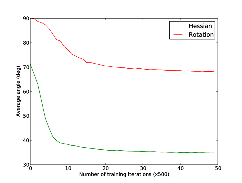
In order to confirm our hypothesis, we ran our algorithm on synthetic and natural Hessian matrices. Synthetic matrices are obtained by randomly drawing rotations and eigenvalues, while the natural matrix we tried is the Hessian of the MNIST dataset.

To evaluate the quality of the approximation, we measure the average angle between the $QDQ^{T}x$ and $Hx$ for a set of random vectors $x$.

The synthetic matrices $H$ are generated as $R\Lambda R^{T}$ where $R$ is a random rotation matrix, uniformly drawn on the set of rotation matrices, and $\Lambda=\mathrm{diag}(\lambda_{i})$ is a diagonal matrix, with $\lambda_{i}=|\mu_{i}|$ where $\mu_{i}$ is sampled from a zero-mean and $0.1$ Gaussian distribution, except a small number $n_{\mu}$ of randomly selected $\mu_{i}$ that are drawn from a Gaussian of mean $1$ and variance $0.4$.
The results are displayed on Figure 1. The average angle goes down to about $35$ degrees in a space of dimension $64$, with the number of large eigenvalues $n_{\mu}=5$.

For sanity check purposes, we also try directly learning a random rotation matrix $R$ using a single $Q$ matrix. The loss function is then

$$\mathcal{L}^{\prime}(w)=\sum_{j}||Qx^{(j)}-Rx^{(j)}||_{2}^{2}$$ (7)

The results are also shown on Figure 1. It doesn’t perform as well as learning a Hessian, which was expected since we don’t have eigenspaces of high dimension, but it still reaches $68$ degrees in dimension $64$.
We performed another sanity check : if the matrix $R$ is actually the form of a matrix $Q_{\omega}$, then we learn it correctly (loss function $\mathcal{L}^{\prime}$ reaching zero), and we also learn $H=R^{T}\Lambda R$ with loss function $\mathcal{L}$ going quickly to zero.

Figure 1: Average error angle versus epochs for matrix learning. In green, learning $H$, with the number of larger eigenvalues $n_{\mu}=5$. In red, learning a rotation matrix $R$.

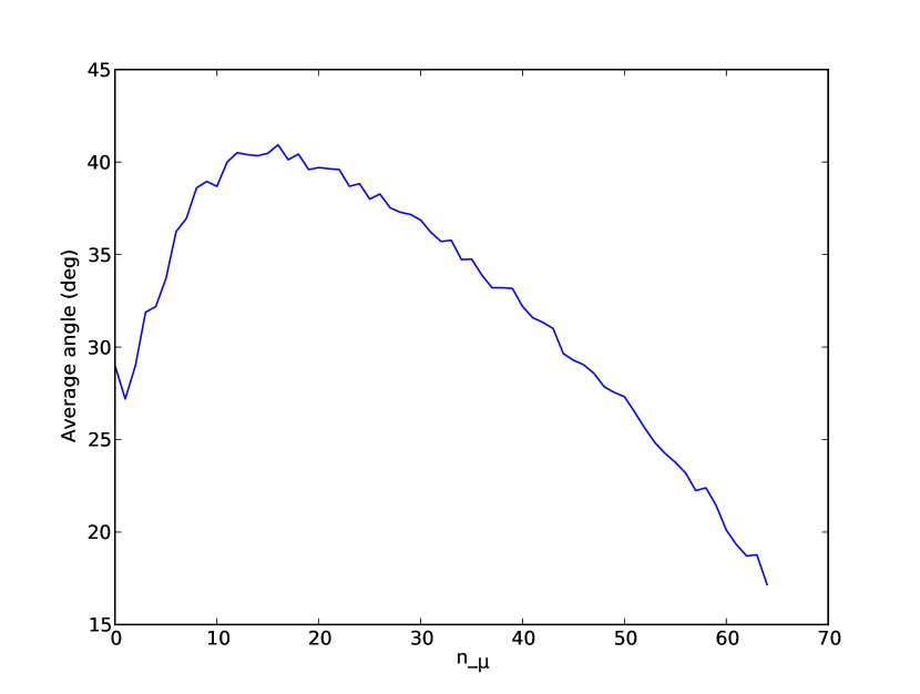
It appears that the number of larger eigenvalues $n_{\mu}$ has an influence on the quality of the approximation : the average error angle after convergence is lower when $n_{\mu}$ is close to $0$ or to the size of the space (about $20$ degrees in the latter case). On the other hand, when the eigenvalues get split into two groups of about the same size, the average error angle can is about $41$ degrees. The average angle as a function of $n_{\mu}$ is shown on Figure 2.

Figure 2: Average error angle after convergence versus the number of dominant eigenvalues $n_{\mu}$.

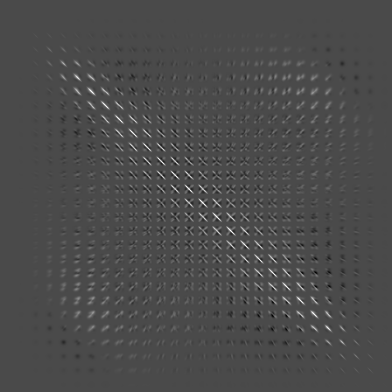
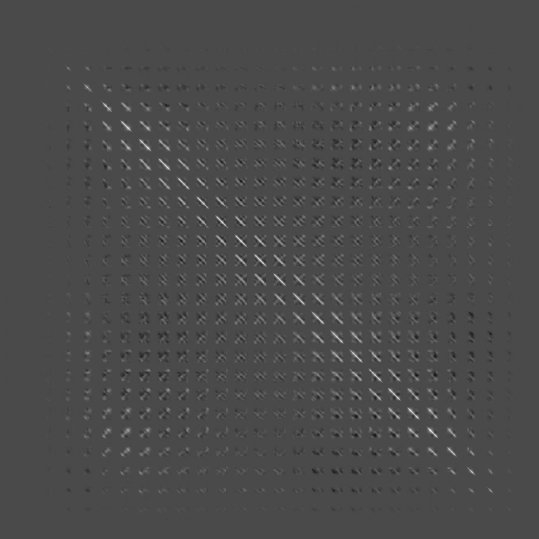
We tested our algorithm on the covariance of the MNIST dataset. It reached an angle of $38$ degrees. Figure 3 shows real and approximated covariance matrices.

Figure 3: True (left) and approximated (right) covariance matrix of the MNIST dataset.

4 Hessian matrices of loss functions

In this section, we denote $\widehat{H}=Q^{T}DQ$ (or $\widehat{H}_{{\widetilde{\omega}}}=Q^{T}_{{\widetilde{\omega}}}D_{{\widetilde{\omega}}}Q_{{\widetilde{\omega}}}$) the approximated Hessian.

4.1 Batch gradient descent

Although learning an approximation of a fixed Hessian matrix has uses, our method can be used in an online fashion to track slowly-varying Hessian matrices over the course of an optimization procedure.

In numerous cases, we have an optimization problem involving too many variables to explicitly compute the Hessian, preventing us from using direct second order methods. Our Hessian representation can be used to store and evaluate the Hessian matrix. Thanks to the learning procedure involved, if the Hessian of the loss function changes, our estimation will be able to adapt.

Let us consider an optimization problem where we aim to minimize a loss function $\ell(u)$ where $u\in\mathbb{R}^{n}$ is the set of parameters. Therefore, we are looking for

$$u^{*}=\underset{u\in\mathbb{R}^{n}}{\arg\min}\ \ell(u)$$ (8)

Or, in case of a non convex problem, we are looking for a $u^{\dagger}$ that gives a “low” value for $\ell$ (“low” being problem dependent).
In addition, let us suppose we are in a case where it is possible to compute the gradient $\nabla_{u}\ell$ of $\ell$ at every point $u$. It is the case, for instance, for neural networks, using the backpropagation algorithm, or whenever we have an efficient way to compute the gradient.

It is well known that even if the problem is quadratic, and therefore the Hessian matrix $H$ doesn’t depend on the point $u$, a gradient descent algorithm can perform poorly when $H$ has eigenvalues with different magnitude. This situation becomes even worse when the loss function is not quadratic in the parameters and the Hessian is not constant (we use notation $H_{u}$ for the Hessian matrix at point $u$). However, if $H_{u}$ is known, we can replace the gradient step $\nabla_{u}\ell$ by $H_{u}^{-1}\nabla_{u}\ell$. This modifies the descent direction to take the curvature into account and allows quadratic convergence if the function is locally quadratic. Since $H_{u}$ is too large to compute or store, we can rely on approximations, such as in LBFGS or Truncated Conjugate Gradient.

Our method provides another way to track an approximation of $H_{u}$. By definition, we have

$$H_{u+\mathrm{d}{}u}\mathrm{d}u=\nabla_{u+\mathrm{d}{}u}\ell-\nabla_{u}\ell+o(||\mathrm{d}u||)$$ (9)

In the context of minimization, let us suppose we have taken a step from point $u_{t-1}$ and arrived at the current point $u_{t}$. Then we know that

$$H_{u_{t}}(u_{t}-u_{t-1})\approx\nabla_{u_{t}}\ell-\nabla_{u_{t-1}}\ell$$ (10)

We can use this relation as a training sample for the matrix $H$.

Thus, we start with an approximated matrix $H_{u_{0}}$ set to identity, and we begin a regular gradient descent. At each step, we obtain a training point as defined in Equation 10, and we perform one step in learning $H_{u_{1}}$ (following the gradient of the loss function $L$). Then we perform a second step in the minimization of $\ell$, folloing vector $H_{u_{1}}^{-1}\cdot\nabla_{u_{1}}\ell$, and so on. Note that our representation of $H_{u_{t}}$ allows us to compute the inverse easily. The procedure is summarized in Algorithm 2.

Algorithm 2 Optimization with linearithmic Hessian

  Parameters: Learning rates $\alpha$ and $\beta$

  Initialize ${\widetilde{\omega}}$ such that $D_{{\widetilde{\omega}}}=I$ and $Q_{{\widetilde{\omega}}}\in\mathcal{Q}$

  Initialize random $u_{0}$

  Set $t=0$

  while not converged do

     Compute $\nabla_{u_{t}}\ell$

     if $t\neq 0$ then

        Set $\delta u=u_{t}-u_{t-1}$

        Set $\delta g=\nabla_{t}\ell-\nabla_{t-1}\ell$

        Update ${\widetilde{\omega}}\leftarrow{\widetilde{\omega}}-\alpha\frac{\partial L({\widetilde{\omega}},\delta u,\delta g)}{\partial{\widetilde{\omega}}}$

        Project $Q_{{\widetilde{\omega}}}$ on $\mathcal{Q}$ as in Equation 6

     end if

     Set $u_{t+1}=u_{t}-\beta\widehat{H}_{{\widetilde{\omega}}}\nabla_{u}\ell$

     Update $t\leftarrow t+1$

  end while

A number of implementation details must be considered :

• It appears that in natural Hessians, many of the eigenvalues are small or zero, especially when we approach a local minimum. Therefore, the inverse of $D$ can diverge. We solve this issue by imposing a minimal value $\epsilon$ on the elements of $D$ when computing their inverse.

• Similarly, eigenvalues can be negative. It is a problem in the minimization since it makes second order methods diverge if not taken into account. There are several ways to deal with such eigenvalues. We chose to set negative elements of $D$ to $\epsilon$ at the same time as the normalization of $Q_{{\widetilde{\omega}}}$.

• The norm of $\delta u$ (as defined in Algorithm 2) can vary from one step to the other. However, since the Hessian approximation is linear, scaling $\delta u$ and $\delta g$ by the same factor is equivalent to scaling the learning rate $\alpha$ by the same factor. To have a better control on the learning rate, we rescale both $\delta u$ and $\delta g$ by a factor $1/||\delta u||$.

Although it performs poorly, due to the small eigenvalues, it is also possible to directly learn the inverse Hessian matrix using the relation

$$\delta u\approx H_{u}^{-1}\delta g$$ (11)

4.2 Stochastic and minibatch gradient descent

For most problems, stochastic gradient descent (SGD) performs better than batch descent. Here, we will consider the intermediate case, minibatch descent, where each step uses only a part of the dataset. It covers both plain SGD and batch methods by setting the size of the minibatch to $1$ or to the size of the dataset.

In minibatch setting, the loss function becomes $\ell_{A}(u)$, where $A$ is a subset of the dataset, changing at each iteration. We have $\ell_{A}(u)=\ell(u)$ if $A$ is the whole dataset. Because of this difference, the previous analysis doesn’t hold anymore, since the Hessian of $\ell_{A}$ is not going to be the same as the Hessian of $\ell_{A^{\prime}}$.

However, we will see that if we use the Hessian learning in this setting, it still perform something very similar to minibatch gradient, on the Hessian approximation. When learning the approximation, instead of training pairs $(\delta u,\delta g)$, we now obtain pairs $(\delta u,\delta g_{A})$, where $\delta u=u_{t}-u_{t-1}$ and $\delta g_{A}=\nabla_{u_{t}}\ell_{A}-\nabla_{u_{t-1}}\ell_{A}$. Let $\mathcal{A}$ be the whole dataset and $(A_{i})_{i=1..p}$ be minibatches (so $A_{i}\subset\mathcal{A}$). Since the gradient operator is linear, if $\mathcal{A}=\uplus_{i=1}^{p}A_{i}$, then

$$\nabla_{u}\ell=\frac{1}{|\mathcal{A}|}\sum_{i=1}^{p}\nabla_{u}\ell_{A_{i}}$$ (12)

This simply states that if we sum gradients, taken at the same point, from a set of minibatches such that the dataset is their disjoint union, then we obtain the batch gradient. We have scaled the batch gradient by the size of the dataset for clarity purposes in the following part.

We will show that the same property holds for the loss function $L$. The loss function for the Hessian approximation corresponding to minibatch $A_{i}$ is $L({\widetilde{\omega}},\delta u,\delta g_{A_{i}})$. Its gradient is

$$\frac{\partial L({\widetilde{\omega}},\delta u,\delta g_{A_{i}})}{\partial{\widetilde{\omega}}}=2\frac{\partial\widehat{H}_{\widetilde{\omega}}}{\partial{\widetilde{\omega}}}\delta u(\widehat{H}_{\widetilde{\omega}}\delta u-\delta g_{A_{i}})$$ (13)

So we get

$$\frac{1}{|\mathcal{A}|}\sum_{i=1}^{p}\frac{\partial L({\widetilde{\omega}},\delta u,\delta g_{A_{i}})}{\partial{\widetilde{\omega}}}$$ (14)

$$= 2\frac{\partial\widehat{H}_{\widetilde{\omega}}}{\partial{\widetilde{\omega}}}\delta u(\widehat{H}_{\widetilde{\omega}}\delta u-\sum_{i=1}^{p}\delta g_{A_{i}})$$ (15)

$$= 2\frac{\partial\widehat{H}_{\widetilde{\omega}}}{\partial{\widetilde{\omega}}}\delta u(\widehat{H}_{\widetilde{\omega}}\delta u-\delta g_{\mathcal{A}})$$ (16)

$$= \frac{\partial L({\widetilde{\omega}},\delta u,\delta g_{\mathcal{A}})}{\partial{\widetilde{\omega}}}$$ (17)

Another issue with minibatch descent lies in the difficulty to reuse the gradient computed at step $t-1$ to compute $\delta g$ at step $t$. Indeed, $\delta g_{A_{i}}=\nabla_{u_{t}}\ell_{A_{i}}-\nabla_{u_{t-1}}\ell_{A_{i}}$. In the batch method, we had already computed $\nabla_{u_{t-1}}\ell_{A}$ at the previous step, and we could reuse it. With the minibatch approach, the previous step used $\nabla_{u_{t-1}}\ell_{A_{i-1}}$, which is not computed on the same minibatch.
The easiest way to overcome this issue is to recompute $\nabla_{u_{t-1}}\ell_{A_{i}}$ at step $t$, but it implies doubling the number of gradients computed. Although we don’t have a fully satisfying answer to this problem, a possibility to reduce the number of gradients computed would be to use the same minibatch $A_{i}$ a few times consecutively before changing to $A_{i+1}$.

4.3 Performance

The approximated Hessians are sparse matrices with $2n$ coefficients each. They can be efficiently implemented using standard sparse linear algebra, such as spblas. The total number of operations for evaluating an approximate Hessian is $O(n\lg(n))$. If we neglect the fact that sparse matrices involve more operations, one evaluation coses $4n\lg(n)+n$ MulAdd operations. Computing the gradient of $\widehat{H}$ has the same cost, thanks to the backpropagation algorithm. Accumulating the gradients cost another $4n\lg(n)+n$. So tracking the Hessian matrix using our method adds about $12n\lg(n)+3n$ operations at each iteration and, when using minibatches, possibly another gradient evaluation.

In terms of memory, there are $2n\lg(n)+n$ parameters to store, and another $2n\lg(n)+n$ is required to store the gradient of $\widehat{H}$ during learning.

5 Applications and future work

The linearithmic structure makes the Hessian factorization scalable to larger models. In particular, large inference problems invloving Gaussian functions are good candidates for our method. Evaluating a product $x^{T}R^{T}DRx$ is even faster, since it can be rewritten $(Rx)^{T}D(Rx)$, and therefore be performed in $2n\lg(n)+2n$ operations. This is particularly adapted to inference, where it is possible to spend some time to learn the approximate the matrix once and for all. Gaussian mixture models and Bayesian inference with Gaussian models could profit from this approximation.

Although some work has still to be done, speeding up optimization by tracking the approximated Hessian could help optimizing function. In particular, deep neural network could profit from this method, since their loss function tend to be non isotropic, so they could profit from fast approximated second order methods.

References

- BBG [09] Antoine Bordes, Léon Bottou, and Patrick Gallinari. Sgd-qn: Careful quasi-newton stochastic gradient descent. Journal of Machine Learning Research, 10:1737–1754, July 2009.
- Ben [13] Gérard Ben Arous. personal communication, 2013.
- BL [89] S. Becker and Y. LeCun. Improving the convergence of back-propagation learning with second-order methods. In D. Touretzky, G. Hinton, and T. Sejnowski, editors, Proc. of the 1988 Connectionist Models Summer School, pages 29–37, San Mateo, 1989. Morgan Kaufman.
- CE [11] Olivier Chapelle and Dumitru Erhan. Improved preconditioner for hessian free optimization. In NIPS Workshop on Deep Learning and Unsupervised Feature Learning, 2011.
- DCM+ [12] Jeffrey Dean, Greg Corrado, Rajat Monga, Kai Chen, Matthieu Devin, Quoc Le, Mark Mao, Marc’Aurelio Ranzato, Andrew Senior, Paul Tucker, Ke Yang, and Andrew Ng. Large scale distributed deep networks. In P. Bartlett, F.C.N. Pereira, C.J.C. Burges, L. Bottou, and K.Q. Weinberger, editors, Advances in Neural Information Processing Systems 25, pages 1232–1240. 2012.
- Gen [98] A. Genz. Methods for generating random orthogonal matrices. In H. Niederreiter and J. Spanier, editors, Monte Carlo and Quasi-Monte Carlo Methods, page 199–213. Springer, 1998.
- GLC [11] Guangzhi Cao, Leonardo R. Bachega, and Charles A. Bouman. The sparse matrix transform for covariance estimation and analysis of high dimensional signals. IEEE Trans. on Image Processing, 20(3):625–640, 2011.
- LBOM [98] Y. LeCun, L. Bottou, G. Orr, and K. Muller. Efficient backprop. In G. Orr and Muller K., editors, Neural Networks: Tricks of the trade. Springer, 1998.
- LSP [93] Y. LeCun, P. Simard, and B. Pearlmutter. Automatic learning rate maximization by on-line estimation of the hessian’s eigenvectors. In S. Hanson, J. Cowan, and L. Giles, editors, Advances in Neural Information Processing Systems (NIPS 1992), volume 5. Morgan Kaufmann Publishers, San Mateo, CA, 1993.
- MSS [12] James Martens, Ilya Sutskever, and Kevin Swersky. Estimating the hessian by back-propagating curvature. In Proc of ICML, 2012. arXiv:1206.6464.
- NCL+ [11] Jiquan Ngiam, Adam Coates, Ahbik Lahiri, Bobby Prochnow, Andrew Ng, and Quoc V Le. On optimization methods for deep learning. In Proceedings of the 28th International Conference on Machine Learning (ICML-11), pages 265–272, 2011.
- Noc [80] Jorge Nocedal. Updating quasi-newton matrices with limited storage. Mathematics of computation, 35(151):773–782, 1980.
- SYG [07] Nicol Schraudolph, Jin Yu, and Simon Günter. A stochastic quasi-newton method for online convex optimization. In Proc. 11th Intl. Conf. on Artificial Intelligence and Statistics (AIstats), pages 433–440. Society for Artificial Intelligence and Statistics, 2007.