Bézier projection: a unified approach for local projection and quadrature-free refinement and coarsening of NURBS and T-splines with particular application to isogeometric design and analysis
Abstract
We introduce Bézier projection as an element-based local projection methodology for B-splines, NURBS, and T-splines. This new approach relies on the concept of Bézier extraction and an associated operation introduced here, spline reconstruction, enabling the use of Bézier projection in standard finite element codes. Bézier projection exhibits provably optimal convergence and yields projections that are virtually indistinguishable from global projection. Bézier projection is used to develop a unified framework for spline operations including cell subdivision and merging, degree elevation and reduction, basis roughening and smoothing, and spline reparameterization. In fact, Bézier projection provides a quadrature-free approach to refinement and coarsening of splines. In this sense, Bézier projection provides the fundamental building block for -adaptivity in isogeometric analysis.
keywords:
Bézier extraction, spline reconstruction, isogeometric analysis, local refinement and coarsening, local projection, quasi-interpolation1 Introduction
Projection is a ubiquitous operation in numerical analysis and scientific computing. Consequently, there is a great need to develop projection technologies that are cheap, accurate, and reliable. This is particularly true in isogeometric analysis where the spline basis may not be interpolatory. In this paper we present Bézier projection, a methodology for local projection (i.e., quasi-interpolation) onto and between spline spaces. Bézier projection converges optimally, is virtually indistinguishable from global projection (which requires the solution of a global system of equations), and provides a unified framework for quadrature-free refinement and coarsening of B-splines, NURBS, and T-splines. In particular Bézier projection can accommodate
-
1.
(Cell) Subdivision or -refinement,
-
2.
(Cell) Merging or -coarsening,
-
3.
(Degree) Elevation or -refinement,
-
4.
(Degree) Reduction or -coarsening,
-
5.
(Basis) Roughening or -refinement,
-
6.
(Basis) Smoothing or -coarsening,
-
7.
Reparameterization or -adaptivity.
These operations can be combined in a straightforward fashion to produce isogeometric -adaptivity. Note that only -refinement of T-splines has appeared previously in the literature [84, 81]. Bézier projection is an extension of Bézier extraction [80, 12] in that it is derived entirely in terms of Bézier elements and element extraction operators. This means it can be applied to existing finite element frameworks in straightforward fashion as an element-level technology. Additionally, we formulate Bézier projection in terms of Kronecker products facilitating its application in high-dimensional settings.
Potential applications of Bézier projection are varied and include:
-
1.
Curve and surface fitting,
-
2.
Mesh adaptivity,
-
3.
Enforcement of boundary conditions,
-
4.
Solution methods with nonconforming meshes,
-
5.
Multi-level solver technology,
-
6.
Data compression for image, signal, and data processing.
In the following, we briefly give a basic background on the building blocks of our approach, namely isogeometric analysis, NURBS and T-splines, and quasi-interpolation. We additionally present a summary of our paper.
1.1 Isogeometric analysis
Isogeometric analysis [51, 23] is a generalization of finite element analysis which improves the link between geometric design and analysis. The isogeometric paradigm is simple: the smooth spline basis used to define the geometry is used as the basis for analysis. As a result, exact geometry is introduced into the analysis. The smooth basis can be leveraged by the analysis [39, 52, 24] leading to innovative approaches to model design [21, 95, 64], analysis [76, 82, 78, 8], optimization [94], and adaptivity [5, 36, 83, 83].
Many of the early isogeometric developments were restricted to NURBS but the use of T-splines as an isogeometric basis has gained widespread attention across a number of application areas [5, 80, 81, 91, 90, 13, 8, 76, 82, 86, 32, 49, 6, 16, 45]. Particular focus has been placed on the use of T-spline local refinement in an analysis context [79, 81, 13, 90, 91].
1.2 B-splines, NURBS, T-splines, and more
Bézier curves and surfaces [30, 10, 11], B-splines [27, 74], and NURBS [92, 71, 72] have become the standard for computer graphics and computer-aided design [71]. This ubiquity has driven the development of many spline-based algorithms. Important examples include knot insertion and knot removal [20, 46, 72, 37] to subdivide and merge cells in the mesh as well as modify the smoothness of the spline functions and degree elevation and reduction [73, 50, 72] to modify the polynomial degree of the basis.
T-splines, introduced in the CAD community [85], are a generalization of non-uniform rational B-splines (NURBS) which address fundamental limitations in NURBS-based design. For example, a T-spline can model a complicated design as a single, watertight geometry and are also locally refineable [84, 81]. Since their advent they have emerged as an important technology across multiple disciplines and can be found in several major commercial CAD products [1, 2]. Recent developments include analysis-suitable T-splines [63, 81, 7, 26, 62], and their hierarchical extension [38].
We note that while NURBS and T-splines have become standard technology in IGA there exist a growing number of alternative spline technologies which have been proposed as a basis for IGA. These are not considered in this paper however it should be noted that Bézier projection can be used in all of these cases for which Bézier extraction can be defined. Hierarchical B-splines [42, 93, 77, 43, 57, 44, 9] are a multi-level extension of B-splines. B-spline forests [83] are a generalization of hierarchical B-splines to surfaces and volumes of arbitrary topological genus. Subdivision surfaces generalize smooth B-splines to arbitrary topology [18, 65, 48, 19, 17]. Splines posed over triangulations have been pursued in the context of piecewise quadratic Powell-Sabin splines [88, 87], and Bézier triangles [53]. Polynomial splines over hierarchical T-meshes (PHT-splines) [31, 60, 61, 59], modified T-splines [56], and locally refined splines (LR-splines) [34, 15] are closely related to T-splines with varying levels of smoothness and approaches to local refinement. Generalized B-splines [67, 22] and T-splines [14] enhance a piecewise polynomial spline basis by including non-polynomial functions, typically trigonometric or hyperbolic functions.
1.3 Quasi-interpolation and local least-squares projection
Quasi-interpolation methods were originally developed as an efficient means to obtain spline representations [29, 28, 58, 3, 75, 22]. Bézier projection can be viewed as an extension or generalization of the integral quasi-interpolants presented by Sablonnière [75]. Interested readers are referred to Sablonnière [75] for an overview and classification of quasi-interpolation methods.
The technique for projection onto a spline basis that is most closely related to our work is the local least-squares projection method of Govindjee et al. [47] in which local projections onto the spline basis over an element are computed and then averaged to obtain a global control value. The averaging step in the method of Govindjee et al. was not presented as an average, but rather as the application of the pseudoinverse of the assembly operator to the control values computed for the elements. It can be shown that this is equivalent to a simple average of the local values and hence the local least-squares projection method can be viewed as a special case of Bézier projection.
1.4 Summary of the paper
In Section 2 required notation and conventions are established. The Bernstein basis is defined along with expressions to relate Bernstein basis polynomials over different intervals. Expressions for the Gramian matrix of the Bernstein basis and its inverse are also given. B-splines and NURBS are defined and an informal presentation of two-dimensional T-splines is given. Bézier extraction is presented and the element reconstruction operator is defined as the inverse of the element extraction operator.
Section 3 introduces Bézier projection as a localized projection operation related to quasi-interpolation. A proof of the optimal convergence of the method is given in Appendix A. The Bézier projection method has three distinct steps.
-
1.
A function is projected onto the Bernstein basis over each element in the mesh.
-
2.
An element reconstruction operator is used to compute the representation of the Bézier curve, surface, or volume in terms of the spline basis functions over each element.
-
3.
The local spline coefficients are averaged to obtain the coefficients or control values of the global basis.
Several applications of the method are given including lifting of the normal field of a spline surface and projection between nonconforming meshes.
Section 4 focuses on Bézier projection between spline spaces. The element extraction operator and the spline element reconstruction operator are used to develop quadrature-free algorithms for knot insertion, knot removal, degree elevation, degree reduction, and reparameterization. The Bézier projection algorithms developed are summarized in Table 2. Simple one-dimensional examples are given for all spline operations in the associated sections.
| Operation | Algorithmic Description | ||||
| General projection |
|
||||
|
degree elevation
-refinement |
B-splines/NURBS Algorithm 4.4 T-splines Algorithm 4.6 | ||||
|
degree reduction
-coarsening |
B-splines/NURBS Algorithm 4.5 T-splines Algorithm 4.7 | ||||
|
knot insertion
basis roughening -refinement |
B-splines/NURBS Algorithm 4.9 T-splines Algorithm 4.11 | ||||
|
knot removal
basis smoothing -coarsening |
B-splines/NURBS Algorithm 4.10 T-splines Algorithm 4.12 | ||||
|
knot insertion
cell subdivision -refinement |
B-splines/NURBS Algorithm 4.13 T-splines Algorithm 4.15 | ||||
|
knot removal
cell merging -coarsening |
B-splines/NURBS Algorithm 4.14 T-splines Algorithm 4.16 | ||||
|
reparameterization
-refinement |
B-splines, NURBS, Algorithm 4.17 and T-splines |
2 Notation and preliminaries
2.1 Univariate Bernstein basis
The univariate Bernstein basis functions are defined as
| (1) |
where and the binomial coefficient , . We choose to define the Bernstein basis over the biunit interval to facilitate Gaussian quadrature in finite element analysis rather than use the CAGD convention where the Bernstein polynomials are defined over the unit interval . The univariate Bernstein basis has the following properties:
-
1.
Partition of unity.
-
2.
Pointwise nonnegativity.
-
3.
Endpoint interpolation.
-
4.
Symmetry.
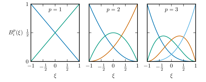
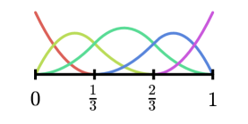
The Bernstein basis functions for polynomial degrees are shown in Fig. 1.
It is often useful to define a vector of basis functions
| (2) |
The degree superscript is suppressed when unnecessary.
Lemma 2.1.
The Bernstein polynomials of degree are linearly independent and form a complete basis for the polynomials of degree over the biunit interval.
We denote the space of functions over the biunit interval spanned by the Bernstein basis of degree by . A useful review of Bernstein polynomials and their properties is provided by Farouki [40].
2.2 Multivariate Bernstein basis
We define a multivariate Bernstein basis over the box of dimension , , by the tensor product. The polynomial degree may be different in each direction and so we define the vector of degrees . The vector of multivariate Bernstein basis functions is defined by the Kronecker product
| (3) |
Thus, there are basis functions in the vector. All of the properties of the univariate Bernstein basis are inherited by the multivariate Bernstein basis. For two dimensions, the Bernstein basis functions can be indexed by the map
| (4) |
so that
| (5) |
where . For the trivariate case we have that
| (6) |
where with the map
| (7) |
2.2.1 Relations between Bernstein polynomials over different intervals
The Bernstein polynomials over the interval are
| (8) |
Given another interval , the Bernstein polynomials are
| (9) |
A polynomial function of degree can be represented by a linear combination of the Bernstein polynomials over or by a combination of the Bernstein polynomials over
| (10) |
As shown by Farouki and Neff [41], the coefficient vectors and can be related by the transformation matrix
| (11) |
where the entries of are given by
| (12) |
This can be extended to multiple dimensions by a tensor product. The elements of the inverse of are given by
| (13) |
The inverse matrix provides a relationship between the basis functions over each interval
| (14) |
Both Eqs. 12 and 13 are defined using one-based indexing for both the matrix entries and the Bernstein basis as opposed to the zero-based indexing used by Farouki and Neff [41].
2.2.2 The Gramian of the Bernstein basis and its inverse
When computing the projection of an arbitrary function onto the Bernstein polynomials, an expression for the Gramian matrix for the basis of degree is required. The entries in the matrix are
| (15) |
Expressions for products and integrals of the Bernstein polynomials given by Doha et al. [33], Farouki [40] permit Eq. 15 to be written in closed form as
| (16) |
The polynomial degree will generally be suppressed. The Gramian matrix for a multivariate Bernstein basis of dimension and with the vector of polynomial degrees is obtained from a Kronecker product
| (17) |
An expression for the inverse of the Gramian of the Bernstein basis can be obtained by considering the Bernstein-Bézier representation of the dual basis given by Jüttler [55]. The Bézier coefficients of the dual basis are precisely the entries in the inverse of the Gramian and so the expression for the dual basis can be used to obtain
| (18) |
after modification to use one-based indexing and the Bernstein basis over the biunit interval. The inverse of a Kronecker product of matrices is given by the Kronecker product of the inverses and so Eq. 18 can be used to compute the inverse of a multivariate Gramian matrix
| (19) |
2.3 Univariate spline basis
A univariate spline is defined by the polynomial degree of the spline and the knot vector , a set of non-decreasing parametric coordinates , where is the number of spline basis functions. We require that the knot vector be open, that is the first knots are equal and the last knots are equal . The th spline basis function over the knot vector is defined using the Cox-de Boor recursion formula:
| (20) |
| (21) |
It is also possible to associate a local knot vector with each spline basis function. The local knot vector is the set of knots chosen contiguously from the knot vector that defines the function . Application of the Cox-de Boor recursion formula to the local knot vector produces the basis function and so it is also possible to index a basis function by its local knot vector:
| (22) |
The B-spline basis enjoys the following properties:
-
1.
Partition of unity.
-
2.
Pointwise nonnegativity.
-
3.
Global linear independence.
-
4.
Local linear independence. Given an open set the B-spline basis functions having some support in are linearly independent on .
-
5.
Compact support.
-
6.
Control of continuity. If has multiplicity (i.e., ), then the basis functions are -continuous at . When , the basis is and interpolatory at that location.
It is interesting to observe that the Bernstein basis defined previously is the set of spline functions given by the knot vector
| (23) |
As with the Bernstein basis, it is possible to define a vector of basis functions
| (24) |
Note that the number of basis functions is less than the number of knots in the knot vector . The space of functions spanned by the functions in is called a spline space.
A spline curve of dimension is a function mapping to . The curve is defined by a set of dimensional control points as
| (25) |
Due to the variation diminishing property of the spline basis, the curve will generally only interpolate the control points at the ends of the curve or at locations where the spline basis is . An alternate form of Eq. 25 can be obtained by defining the vector of control points so that
| (26) |
The vector of control points can be interpreted as a matrix of dimension .
2.4 Rational univariate splines
The spline basis defined in the previous section provides a flexible means to represent curves, however certain curves of interest such as circular arcs cannot be represented by a polynomial basis. A rational spline basis can be used to remedy this deficiency. The rational basis is defined by associating a weight with each basis function and introducing the weight function
| (27) |
The rational basis functions are then defined as
| (28) |
and a rational curve is defined as
| (29) |
A rational curve of this type is commonly referred to as a Non-Uniform Rational B-Spline (NURBS) curve. It is customary to represent the rational curve by a polynomial curve in a dimensional space known as a projective space. The control points are converted to so-called homogeneous form . This definition permits the definition of the -dimensional polynomial curve
| (30) |
This construction permits the application of standard B-spline algorithms to rational spline curves. Therefore all of the algorithms in this paper can be applied to rational splines.
2.5 Multivariate spline basis
Just as the multivariate Bernstein basis is defined by a tensor product of the univariate basis, a multivariate spline basis is defined from a tensor product of univariate spline bases. The univariate spline basis in each parametric direction are defined by a polynomial degree and a knot vector . The number of parametric dimensions is denoted by . The total number of basis functions in the spline basis is given by
| (31) |
where is the number of univariate spline basis functions in the th parametric dimension.
For two dimensions, we define the map and the th basis function is then given by
| (32) |
Similarly, for three dimensions, and the th basis function is given by
| (33) |
It is also possible to define a single basis function in terms of the local knot vectors that define the function in each parametric direction:
| (34) |
Here is the th set of contiguous entries in the knot vector that defines the spline in the first parametric dimension and is similarly chosen from . A vector of spline basis functions can be define by a Kronecker product of the vectors of univariate basis functions:
| (35) |
A multivariate rational spline basis can be defined in the same manner as the univariate case.
Spline surfaces and volumes can be constructed by associating a control point with each basis function. The geometric map is defined as the sum of the product of control points and spline basis functions:
| (36) |
where is a spatial position vector and is a parametric position vector. The geometric map is given in matrix form as
| (37) |
where is the vector of control points.
The geometric map is a bijective map from the parametric domain , which defines the spline, to the physical or spatial domain . Due to the convex hull property of splines, the spatial domain is contained in the convex hull of the control points. The geometric map defines the spline surface or volume in physical space and parameterizes it by the parametric coordinates. A rational spline basis can be constructed from these ideas in a manner similar to what is described for the one-dimensional case in Section 2.4.
2.6 T-splines
T-splines represent a generalization of B-splines and NURBS. Whereas a B-spline is constructed from a tensor product of univariate splines, a T-spline permits meshes with hanging nodes or T-junctions. T-splines contain standard B-splines and NURBS as special cases. The theory of T-splines is rich and dynamic. We do not delve deeply into T-spline theory in this paper and instead refer the interested reader to Sederberg et al. [84], Scott et al. [80, 81], Li and Scott [62] and the references contained therein. We limit our discussion to two-dimensional T-splines of arbitrary degree.
2.6.1 The T-mesh
Given polynomial degrees, and , and two index vectors, , , we define the index domain of the T-mesh as . We associate a knot vector , , with the corresponding index vector . Any repeated entries in are referred to as knots of multiplicity . We require that the first and last knots have multiplicity , this is commonly called an open knot vector. We also require that no knot in have multiplicity greater than . It should be noted that repeated knots have unique indices. We define the parametric domain of the T-mesh as .
A T-mesh is a rectangular partition of the index domain such that all vertices have integer coordinates taken from and , all cells are rectangular, non-overlapping, and open, and all edges are horizontal or vertical line segments which do not intersect any cell. Because there are corresponding parametric values assigned to each vertex in the index space, the T-mesh can be mapped to the parametric domain. Cells in the index domain that are bounded by repeated knot values are mapped to cells of zero parametric area in the parametric domain. An example T-mesh is shown in Fig. 2. Cells that are bounded by repeated knots in at least one dimension have zero parametric area and are shown in gray in the figure.
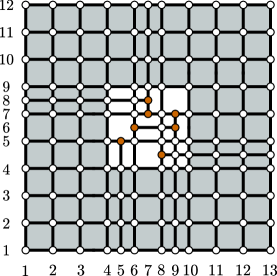
We say that two T-meshes and are nested if can be created by adding vertices and edges to . We use the notation to indicate this relationship.
2.6.2 T-spline basis functions
The T-spline basis functions are constructed from the T-mesh and the knot vectors. Note that we use the term basis function throughout this section although there is no guarantee that the set of blending functions inferred from a T-mesh form a basis for the space. This question is resolved by analysis-suitable T-splines. A basis function is anchored to unique T-mesh entities (i.e., vertices, edges, cells) as follows:
-
1.
If and are odd then the anchors are all the vertices in the T-mesh with indices greater than and less than in the first dimension and greater than and less than in the second dimension.
-
2.
If and are even then the anchors are all the cells in the T-mesh bounded by vertices with indices greater than and less than in the first dimension and greater than and less than in the second dimension.
-
3.
If is even and is odd then the anchors are all the horizontal edges in the T-mesh bounded by vertices with indices greater than and less than in the first dimension and greater than and less than in the second dimension.
-
4.
If is odd and is even then the anchors are all the vertical edges in the T-mesh bounded by vertices with indices greater than and less than in the first dimension and greater than and less than in the second dimension.
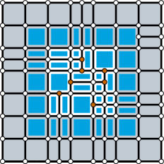
The function anchors for these four cases are illustrated in Fig. 3. We assume that the anchors can be enumerated and refer to each anchor by its index .
 |
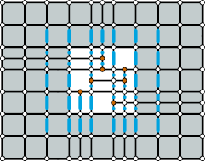 |
| (a) anchors are faces. | (b) anchors are vertical edges. |
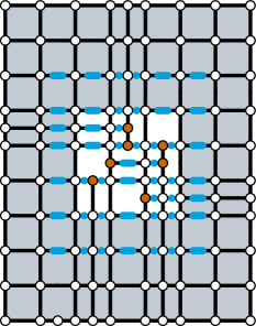 |
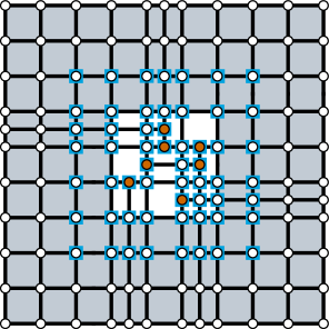 |
| (c) anchors are horizontal edges. | (d) anchors are vertices. |
The basis functions associated with each anchor are defined by constructing a local knot vector in each parametric direction. The function anchor is indicated by its index and so the local knot vector associated with in the th parametric direction is denoted by . The algorithm for constructing the local knot vector in the th parametric direction associated with the th anchor is given here with examples of its application following.
Algorithm 2.2.
Construction of the local knot vector in the th parametric direction for the th function anchor from the T-mesh.
-
1.
Find the line that lies in the th parametric direction and that passes through the center of the function anchor. We refer to this as the anchor line associated with the th parametric direction. This line is used to find the indices that define the local knot vector.
-
2.
Determine the width of the anchor of interest in the direction perpendicular to the anchor line and thicken the line so that it has width and is centered on the anchor line. If the polynomial degree is odd in all directions then and so the anchor line and thickened anchor line coincide.
-
3.
Find the indices of vertices or perpendicular edges in the T-mesh whose intersection with the thickened anchor line is nonempty and of length .
-
4.
The local index vector is the ordered set of indices formed by collecting the closest indices found in the previous step on either side of the anchor . If is odd, then the index of the edge or vertex associated with the anchor is added also to the local index vector. The local index vector is of length .
-
5.
The local knot vector is formed by collecting the knot entries in the global knot vector given by the indices in the local index vector .
By carrying this process out in each parametric direction, a set of local knot vectors associated with the anchor can be obtained. The basis function associated with the anchor is then defined in the same manner as the local spline basis function for B-splines indexed by local knot vectors:
| (38) |
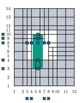
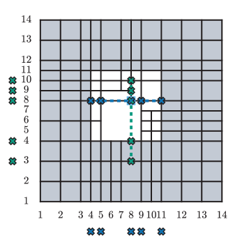
where the functions are obtained by applying the Cox-de Boor formula to the local knot vectors . The process for constructing local knot vectors is illustrated in Fig. 4 for four cases: , , , and .
T-splines with even degree in both directions have cell faces as anchors; thus for the case shown in part (a), the function anchor is marked by a large, light blue box covering the cell face. We use the global knot vectors
| (39) |
and
| (40) |
The anchor line used to construct the horizontal knot vector is shown in dark blue and the anchor line used to construct the vertical knot vector is shown in green. Because the spline has even polynomial degree, the thickened anchor line is shown in both directions. The indices that contribute to the local knot vector are marked with a . The indices used to construct the horizontal local index vector for the marked function are and so the local knot vector for the function is . The indices and were skipped because there are no edges associated with those indices that intersect with the horizontal anchor line used to determine the local knot vector. Note that the index was skipped because the edges that intersect the horizontal line do not span the thickened anchor line due to the missing edge between and . Similarly, the vertical local index vector is and so the vertical local knot vector for the function is .
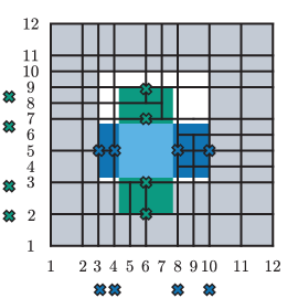 |
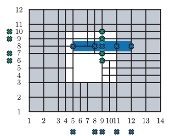 |
| (a) anchors are faces. Thickened anchor lines in both directions. | (b) anchors are vertical edges. Only the horizontal anchor line must be thickened. |
 |
 |
| (c) anchors are horizontal edges. Only the vertical anchor line must be thickened. | (d) anchors are vertices. Neither anchor line must be thickened. |
The mixed degree case is shown in part (b). We now use the global knot vectors
| (41) |
and
| (42) |
Here the function anchor is a vertical edge and so only the horizontal anchor line is thickened (shown in dark blue in the figure). The vertical anchor line is shown as a dashed green line. The horizontal indices that contribute to the local index vector are and so the horizontal local knot vector is . The index is skipped because it does not have edges that span the thickened anchor line at the intersection. It is not necessary to check the span in the vertical direction because the anchor has no width. The vertical index vector is and the vertical local knot vector is .
The opposite mixed degree case is shown in part (c). The global knot vectors are now
| (43) |
and
| (44) |
The function anchors are now horizontal edges and so only the vertical anchor line must be thickened. The indices for the horizontal local index vector are and the knot vector is . The horizontal anchor line has no width perpendicular to the horizontal direction and so only intersections must be checked. The indices for the vertical local index vector are ; here all of the edges intersected span the anchor. The vertical local knot vector is .
The odd degree case is shown in part (d). We choose the global knot vectors
| (45) |
and
| (46) |
For T-splines with odd degree in both directions, the anchors are vertices, the anchor lines are not thickened, and so only intersection must be checked. The indices for the horizontal local knot vector are and the local knot vector is . The indices for the vertical local knot vector are and so the local knot vector is . Once the T-spline basis functions have been defined and control points have been assigned to each one, the geometric map is given by
| (47) |
2.6.3 Face and edge extensions and analysis-suitable T-splines
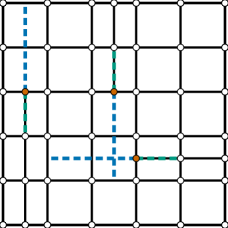
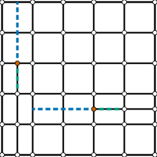
Although the T-spline blending functions defined in this fashion can be used to define smooth surfaces, many properties of the resulting space are not immediately obvious. In order to develop T-splines that are well-characterized and suitable for analysis, we introduce the face and edge extensions of T-junctions. A face extension is a closed line segment that extends from the T-junction in the direction of the face of the cell at which the T-junction terminates and that crosses perpendicular edges or vertices. The edge extension of a T-junction is a closed line segment that extends from the T-junction in the opposite direction of the face extension and that crosses perpendicular edges or vertices. A T-mesh is analysis suitable if no vertical T-junction extension intersects a horizontal T-junction extension. Note that because the edge and face extensions are closed segments, they can intersect at endpoints. The face and edge extensions are shown for a T-mesh that is not analysis-suitable and for an analysis-suitable T-mesh in Fig. 5. The T-mesh formed by adding all face extensions to is called the extended T-mesh and is denoted by .
 |
 |
The T-spline basis defined by an analysis-suitable T-mesh possesses many important mathematical properties including the following theorems [38, 62]:
Theorem 2.3.
The basis functions of an analysis-suitable T-spline are locally linearly independent.
Theorem 2.4.
The basis functions of an analysis-suitable T-spline form a complete basis for the space of polynomials of degree .
Theorem 2.5.
The analysis-suitable T-spline spaces and are nested (i.e., ) if , that is, if can be constructed by adding edges to .
We only consider analysis-suitable T-splines (ASTS) for the remainder of this work. The spline space spanned by a T-spline basis defined by the T-mesh is denoted by .
2.7 Bézier extraction and spline reconstruction
Although analysis-suitable T-splines possess the mathematical properties required by analysis it is not immediately obvious how the basis can be integrated into existing finite-element tools. One of the first issues that must be addressed is how a computational mesh is obtained from the T-mesh. A simple and elegant solution to this problem is based on Bézier extraction introduced in Borden et al. [12] for NURBS and Scott et al. [80] for T-splines. The Bézier mesh is created by adding the face extensions to and then mapping the resulting index mesh to the parametric domain. Note that for ASTS the edges in represent all lines of reduced continuity in the T-spline basis. This makes the Bézier mesh the natural mesh for finite element analysis based on T-splines since the basis is in the interior of each Bézier element. The image of the Bézier mesh under the geometric map (Eq. 47) generates the physical mesh. The Bézier elements for a given mesh can be enumerated and so we refer to the elements by their index . The parametric domain of a Bézier element is denoted by and the physical domain of a Bézier element is denoted by .
Bézier extraction generates the Bernstein-Bézier representation of the T-spline basis over each element. The resulting linear relationship is encapsulated in the so-called Bézier element extraction operator denoted by . Given the control values, , associated with the spline basis functions which are nonzero over element the control values associated with the Bernstein basis defined over the element are related to the spline control values using the transpose of the element extraction operator
| (48) |
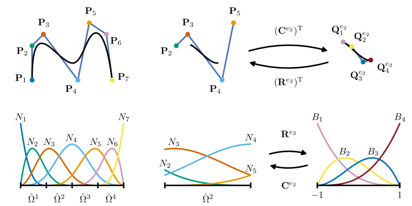
There is an element extraction operator associated with each element in the Bézier mesh. Algorithms for computing the element extraction operators for ASTS and B-splines are given by Borden et al. [12] and Scott et al. [80]. Bézier extraction is graphically demonstrated in Fig. 6. The cubic B-spline curve and control points are shown in the upper left and the corresponding B-spline basis in the lower left. The basis is defined by the knot vector . The segment of the spline curve corresponding to the second element is shown in the middle of the figure with its associated control points. The spline basis supported by the second element is shown below. The Bézier control points produced by the transpose of the element extraction operator are shown in the upper right with the associated Bernstein basis below.
Lemma 2.6.
The Bézier element extraction operators for an analysis-suitable T-spline (and B-splines and NURBS) are invertible.
Proof.
The element extraction operator provides a map from the Bernstein polynomials to the T-spline basis functions over the element. Both sets are linearly independent and complete (Lemmata 2.1 and 2.3), therefore the element extraction operator is invertible. ∎
The inverse of the Bézier element extraction operator and its significance have not been considered previously. It can be seen in Fig. 6 that the inverse transpose of the Bézier element extraction operator provides a means to convert the Bézier control points into spline control points. For this reason, we have termed the inverse of the Bézier element extraction operator the spline element reconstruction operator
| (49) |
or element reconstruction operator for short. Whereas the Bézier element extraction operator “extracts” Bézier coefficients the spline element reconstruction operator converts Bézier coefficients into spline coefficients, thus “reconstructing” the spline segment. Additionally, the element reconstruction operator can be used to express the Bernstein basis in terms of the spline basis defined over element . The element reconstruction operator is a core component of the Bézier projection method developed in this paper.
3 Bézier projection
Given function spaces and , we use to represent the projection from a function in to a function in . If , then the projection is exact or injective. Where the meaning is unambiguous, we use to represent the projection onto or to denote a general projection. The definition of a projector requires that for , .
We define our projection problem as follows: given a function in some function space mapping a domain to and a discrete space of spline functions, , mapping to , find a set of coefficients or functionals (or vector of functionals if ) such that the function given by
| (50) |
where are the basis functions of and is the coefficient associated with the th basis function, approximates in some sense. The optimal projector returns the coefficients that minimize the error with respect to the norm over the domain
| (51) |
where . It is standard to use the norm.
If the domain over which the function is defined does not coincide with the domain over which the spline basis is defined, a function mapping to , must be introduced and the composition is projected onto the spline basis. When projecting onto a spline basis over a geometry, this map is the geometric map that defines the geometry. For simplicity of exposition, in this section we assume that the two domains coincide, that is .
In general, the functionals of the global projection problem require integration over the entire domain and solution of a linear system of the same size as the dimension of the spline space . A localized projection or quasi-interpolation [75] is defined by choosing functionals that can be determined from function values over a subdomain and that do not require the solution of a linear system of the same size as the spline space.
3.1 Formulation of Bézier projection
We introduce Bézier projection as a localized projection operation that uses a linear combination of projections onto the element Bernstein basis. Given a map from the biunit interval to the knot interval (or element) , we define the projector of a function over the interval onto the Bernstein basis over the biunit interval as
| (52) |
where the functionals are obtained from the projection of onto the Bernstein basis of degree . When the meaning is unambiguous, we suppress the superscript for the polynomial degree. Note that the original function is defined over the domain while the definition of local projection presented here introduces a transformation so that the projected segment of is represented over the biunit interval. The functionals with respect to the norm are found from the linear system
| (53) |
where the inner product is defined as
| (54) |
If it would be necessary to introduce an additional transformation . In this case, the second entry in the inner product on the right-hand side of Eq. 53 would be . The solution to Eq. 53 can be written as
| (55) |
by using the inverse of the Gramian matrix and defining the vector of functionals (Bernstein coefficients) and the vector of basis function-function inner products . The inverse of the matrix is given in closed form by Eq. 18 and so the solution can be computed directly without a numerical solution step.
Bézier extraction can be interpreted as a projection of a spline basis function onto the Bernstein basis:
| (56) |
where are the entries of the element extraction operator . Recall that the function is defined over the parametric domain of the spline while the Bernstein representation on the right-hand side of Eq. 56 is defined over the biunit interval. The coefficients of the spline basis functions, denoted by , over element are related to the Bézier coefficients of the Bernstein basis by the element reconstruction operator
| (57) |
3.1.1 Bézier projection weighting scheme
In general, the control value for a given function produced by Bézier projection will be different for each element in the support of the function. These values must be averaged, selected, or combined in some way to generate a unique global control point. We choose to construct the global set of coefficients from a weighted sum of the local coefficients
| (58) |
where contains the elements in the support of the th basis function and represents the coefficient of basis function on element . These results can be combined to express the full Bézier projection as
| (59) |
To guide the development of our weighting scheme we recall that
Lemma 3.1.
For a spline function we have that for all .
Proof.
This follows directly from the definition of Bézier extraction and the element extraction operator and its invertibility. ∎
Lemma 3.2.
If then is a projector.
Proof.
Given a function if the weights do not sum to one then the weighted sum of the local coefficients cannot be equal to the global coefficient and so is not a projector. ∎
We note that by choosing the weights as where is the number of elements in the support of the th basis function, the local least-squares method of Govindjee et al. [47] is obtained; however, it will be seen that the weighting proposed here provides significantly increased accuracy in the results.
A particularly accurate choice of weights is
| (60) |
When projecting a geometry onto a new basis, the spatial domain is not defined and the parametric domain is used instead. The weights obtained by this method for the basis functions defined by the local knot vectors , , , , and are shown in Fig. 7.
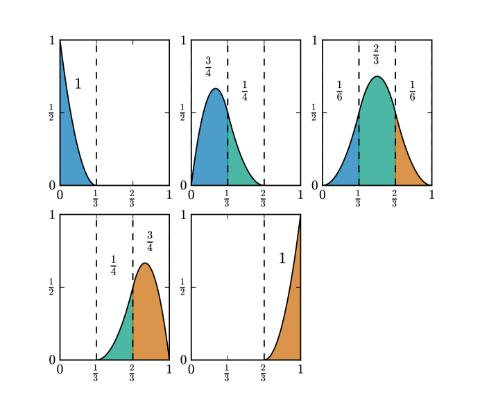
The individual steps comprising the Bézier projection algorithm are illustrated in Fig. 8. The curve defined by , is projected onto the quadratic B-spline basis defined by the knot vector . Because the domain of the curve parameter does not coincide with the parametric domain of the spline, we introduce the affine map and project onto the spline basis using Bézier projection. All of the basis functions are shown in Fig. 7 along with the weight associated with each function over each element. The first step is to perform a projection onto the Bernstein basis for each element to obtain the local Bézier coefficients that define an approximation to the target function over the element. The Bézier control points are indicated in part (1) of the figure by square markers that have been colored to match the corresponding element. The local approximation to the target function is shown along with the control points. Because the local Bézier control points are interpolatory at the ends of the segments, it can be seen from the placement of the Bézier control points associated with adjacent segments that the Bézier curve segments are discontinuous.
Next, the element reconstruction operator is used to convert the Bézier control points into spline control points associated with the basis function segments over each element. This operation does not change the discontinuous segments that approximate the target function, but rather changes the basis used to represent those segments from the Bernstein basis to the spline basis. The new control points are marked with inverted triangles and again colored to indicate the element with which the control point is associated. The control points occur in clusters. The clusters of control points represent the contributions from multiple elements to a single spline basis function control point. The endpoints have contributions from a single element. The points to the right and left of either endpoint have contributions from two elements. It can be seen that the center control point contains contributions from each of the 3 elements of the mesh. Again, the discontinuous nature of the approximation segments can be discerned by observing that the control points are slightly scattered.
Each cluster of control points must be combined (averaged) to obtain a single control point associated with the respective basis function. A weighted average of the points in each cluster is computed using the weighting given in Eq. 60 and the resulting control points are shown as circles with the relative contribution from each element to each control point indicated by the colored fraction of the control point marker. The weights are those from Fig. 7. The colors in Figs. 7 and 8 are coordinated to illustrate where the averaging weights come from and their values. To summarize,
Algorithm 3.3.
Bézier projection onto a spline basis.
-
1.
Compute the projection of the target function onto the Bernstein basis on each element to obtain the vector of local Bézier control values (Eq. 53).
-
2.
Use the transpose of the element reconstruction operator to convert the local Bézier values to spline control values for the element segments (Eq. 57).
- 3.
Alternatively, steps 1 and 2 of Algorithm 3.3 can be combined by projecting the target function directly onto the local segments of the global spline basis.
| (0) |

|
Target function |
|---|---|---|
| (1) |

|
Perform local projection to obtain Bézier control points (represented by squares, colored to match elements) |
| (2) |

|
Use element reconstruction operator to project Bézier points to spline control points (represented by inverted triangles, colored to match elements) |
| (3) |

|
Apply smoothing algorithm (contribution of each element to each control point shown by colored fraction) |
| (4) |

|
Comparison of final function (light blue) and target function (dashed) |
When projecting onto splines with parametric cells that are proportionally similar to the physical elements it may not be necessary for accuracy to compute the physical integrals appearing in Eq. 60. Recall that . Therefore the weight associated with function over element may be approximated by
| (61) |
where represents the volume of the parametric domain associated with element .
3.2 Projection onto a rational basis
When projecting a function onto a rational basis it is assumed that a weight coefficient is given for each basis function. These weight coefficients define the weight function given in Eq. 27. Rather than projecting directly onto the rational basis, we choose to compute a set of homogeneous coefficients . These coefficients are related to the coefficients of the rational basis functions by
| (62) |
Leveraging homogeneous coefficients allows us to use Bézier projection as formulated for projection onto a polynomial spline basis with the exception that the function that we project is . The element extraction operator can be used to convert the spline weight coefficients to Bézier weight coefficients. The Bézier weight coefficients can then be used to compute the weight function over element . In one dimension, the element weight function is
| (63) |
The homogeneous Bézier coefficients over the element are then given by
| (64) |
where is given by Eq. 18 and the entries in the vector are given in one dimension by
| (65) |
The Bézier projection process then proceeds as outlined from Eq. 57 onward with all and variables replaced by their homogeneous counterparts and .
3.3 Convergence
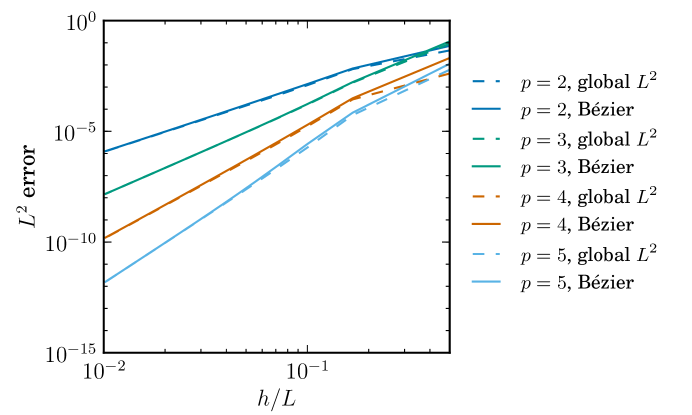
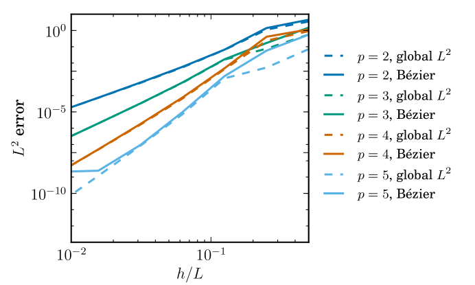
We illustrate the convergence of the Bézier projection method with the weighting defined in Eq. 61 by comparing the error in the global projection to the error in Bézier projection. We use a single cycle of of a sinusoid over the unit interval given by to test the convergence. The error of the projection of the sine function onto a spline basis using Bézier projection is compared to the global projection in Fig. 9 for splines with polynomials degree ranging from 2 to 5. It can be seen that the Bézier projection preserves the optimal convergence rates of the underlying basis for all degrees. Furthermore, the results of Bézier projection converge rapidly to the global projection results with only weak dependence on the polynomial degree of the basis.
We now consider the benchmark problem proposed by Govindjee et al. [47] in which the function
| (66) |
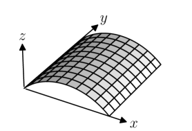
is projected onto the rational spline basis that defines a quarter cylinder of length and radius that is positioned so that one flat edge of the shell lies on the axis with the lower corner at the origin and the other lies in the plane along the line . The geometry is illustrated in part (a) of Fig. 10 and the evaluation of the function on the surface is shown in part (b) of the same figure.
The convergence of the Bézier projection is compared to global projection in Fig. 11. It can be seen that the Bézier projection converges optimally. There is an apparent floor for the convergence of the case that can be attributed to the conditioning of the Bernstein basis and the element extraction operators. Addressing this issue is beyond the scope of this paper but will be treated in a future paper.
 |
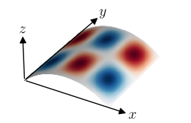 |
| (a) | (b) |
Theorem 3.4.
The Bézier projector exhibits optimal convergence rates.
Proof.
See Appendix A. ∎
3.4 Applications and examples
3.4.1 Lifting of a surface normal field to spline control vectors
For many operations involving surfaces it is advantageous to have an accurate but approximate spline representation of the normal field. The normal field can be approximated by finding a set of “control vectors” that define a vector field over the surface:
| (67) |
The control vectors can be thought of as vectors anchored to the control points that define the surface. We refer to the process of calculating control vectors from a vector field defined over a surface as “lifting” the field off the surface onto the control points. The control vectors which approximate a normal field can be easily computed with Bézier projection.
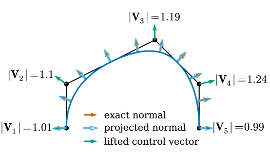
The process is illustrated in Fig. 12. The normal field for the curve is depicted with orange arrows. The control vectors obtained from Bézier projection of the normal field onto the spline basis are shown in green on the associated control points. The magnitute of the control vectors is also shown. It is interesting to note that the control vectors for the approximate normal field have magnitude greater than 1. The approximate projected normal field given by Eq. 67 is represented by the blue empty arrows. The approximate normal field represents the normal field well except in regions of increased curvature. Because the Bézier projection method enjoys optimal convergence rates, the accuracy can be improved by increasing the polynomial degree of the spline basis used to represent the normal field or by subdividing knot intervals.
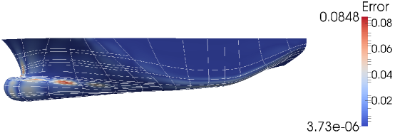
A more complex T-spline normal lifting example is shown in Fig. 13. A smooth containership hull is modeled using bicubic T-splines. The Autodesk T-spline plugin for Rhino is used to model the surface [1] and the Bézier extraction of the surface is then automatically exported for further processing. Note that once the Bézier extraction is computed, no further information from the original CAD model is required. The T-splines in Fig. 13a and Fig. 13c are composed of 36 Bézier elements and 75 control points. The globally-refined T-splines in Fig. 13b and Fig. 13d are composed of 156 Bézier elements and 221 control points. In Fig. 13a the magnitude of the error in the projected normal field is shown. Notice the expected concentration of error in regions of high curvature. To improve the accuracy of the projected normal field the coarse containership hull is globally refined to produce the T-spline in Fig. 13b. Notice the dramatic improvement in the accuracy of the projected normal field. Fig. 13c and Fig. 13d compare the exact normals (blue arrows) to the projected normals (red arrows) at the corners of each Bézier element for the coarse and fine T-spline.
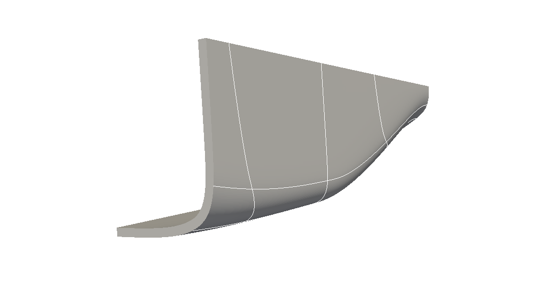
The projected normal field can be used to automatically generate a thickened shell geometry as shown in Fig. 14. We feel that this approach has the potential to provide a rigorous geometric foundation for structural mechanics applications based on plate and shell models.
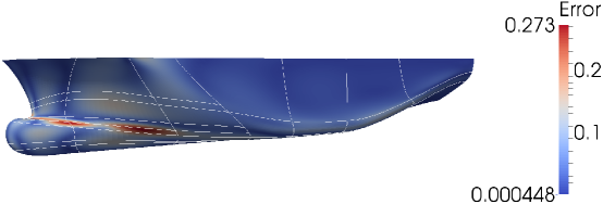 |
| (a) Magnitude of error in projected normals for coarse T-mesh |
|
| (b) Magnitude of error in projected normals for fine T-mesh |

|
| (c) Exact normals (blue arrows) compared to projected normals (red arrows) for coarse T-mesh |

|
| (d) Exact normals (blue arrows) compared to projected normals (red arrows) for fine T-mesh. |
 |
3.4.2 Projection between advected meshes
Another application that benefits significantly from Bézier projection are isogeometric methods that rely on moving or advected meshes. For example, in problems involving flow over moving boundaries or large deformations it is often necessary to move the mesh with the material and/or remeshing of the computational domain. This is a fundamental component of arbitrary Lagrangian-Eulerian (ALE) type methods [35, 54].
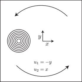
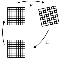
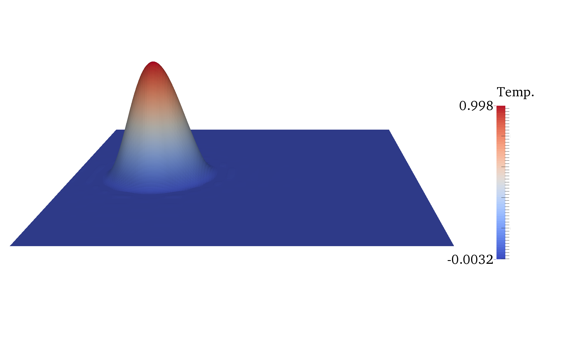
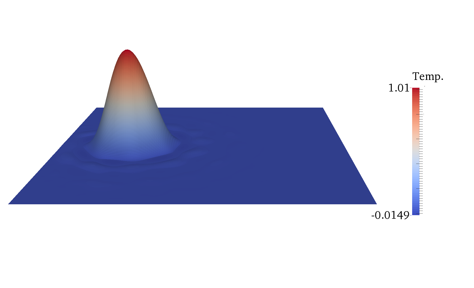
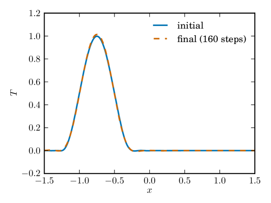
As a simple example of the behavior of Bézier projection for these problems, we consider a benchmark problem of pure advection, namely the advection of a sine bump temperature feature by a rotating flow. The problem statement is given in Fig. 15. Rather than solve the advection problem directly, we employ a moving mesh approach. The mesh and field defined over it are advected with the flow and then periodically projected back onto the the original spatial grid. This procedure is illustrated in Fig. 16. The rotation operator is used to rotate the mesh and field and then a Bézier projection is used to project the field from the rotated mesh onto a spatially aligned grid. Bézier projection is especially advantageous here because only the elements in the rotated mesh that overlap a given element in the spatial mesh are required to perform the integration on each element. After the local integrations have been completed, the result is smoothed using Eq. 60. The process is then repeated until the simulation is complete. The spinning mesh was carried out on a 30 by 30 mesh on a square domain using biquadratic B-splines. The mesh was rotated by at each time step so that 20 steps were required to complete a full rotation. A total of 8 rotations of the cone about the origin were computed using 160 steps. The first and last steps of the simulation are shown in Fig. 17. The 160 steps required to advect the sine bump through 8 rotations have resulted in an increase in over- and undershoot of approximately one percent. A slice through the solution along the axis is shown in Fig. 18. The repeated projections between non-aligned meshes have not produced any observable changes between the initial and final states beyond the slight increase in over- and undershoot.
 |
 |
4 Projection between spline spaces and operations on splines
We now consider Bézier projection between splines spaces. We refer to the spaces and as the source space and target space, respectively. While it is possible to use Bézier projection as defined in Section 3 to project between spline spaces, we will show that it is possible to define a quadrature-free Bézier projection approach for projection between spline spaces. This approach can then be used to obtain algorithms for knot insertion and removal, degree elevation, and reparameterization that can be applied to any spline that can be represented using Bézier extraction (B-splines, NURBS, T-splines, LR-splines, etc.).
In all cases, the algorithms construct a new spline space and then project the original spline representation onto the new space. All of these operations except reparameterization consist of either projection from one space onto a superspace, which we refer to as refinement, or projection from a space onto a subspace, which we refer to as coarsening. It is also possible to define non-nested refinement operations that increase the number of basis functions or degrees of freedom without projecting onto a superspace although this possibility is not considered in great depth here beyond reparameterization.
One of the intriguing new features of the isogeometric paradigm is the potential for -refinement [51, 25], or in other words, adaptively modifying the local smoothness of the basis to improve the accuracy of the solution. Hughes et al. [51] and Cottrell et al. [25] originally used the term -refinement to refer to the process of generating a sequence of smoother and smoother bases. We prefer to use -refinement to denote the process of basis roughening, or reducing the smoothness of a basis through knot insertion, and -coarsening to indicate the smoothing of the basis functions through knot removal. The reason for this convention is twofold. First, we prefer to use the word refinement to indicate the transformation of the solution into a space that contains the unrefined solution. This is not the case for a smoothed basis. A function represented in terms of a spline basis that is at each knot cannot be represented by a basis that has higher continuity at the knots. Second, the word refinement suggests increased resolution or the capability to represent finer detail or additional features. The process of basis smoothing reduces the dimension of the space and so we refer to basis smoothing as -coarsening. The space of spline functions defined by basis roughening contains the original space and provides additional degrees of freedom and so we feel that it is most natural to associate basis roughening with -refinement.
To simplify later developments we adopt the following naming convention:
-
1.
(Cell) Subdivision is -refinement.
-
2.
(Cell) Merging is -coarsening.
-
3.
(Degree) Elevation is -refinement.
-
4.
(Degree) Reduction is -coarsening.
-
5.
(Basis) Roughening is -refinement.
-
6.
(Basis) Smoothing is -coarsening.
-
7.
Reparameterization is -adaptivity.
Bézier projection between spline spaces reduces to a highly localized projection between two different Bernstein bases. It is possible to express this in matrix form as
| (68) |
where the element extraction operator on the source mesh converts the spline coefficients to Bézier form, the matrix converts the Bézier coefficients of the source Bernstein basis into coefficients of the target Bernstein basis, and the element reconstruction operator on the target mesh is used to convert the new Bézier coefficients into spline coefficients for the target basis. The weighted average or smoothing algorithm given in Eq. 58 can then be applied, if necessary, to obtain a set of global coefficients. If the target space is a superspace of the source space, , then the smoothing algorithm is not required and the projection is exact. Otherwise, the projection is approximate. The form of will depend on the particular type of projection being performed (i.e, , , or ).
Leveraging the tensor-product structure of the element extraction and reconstruction operators and the multivariate Bernstein basis, Eq. 68 can also be written as
| (69) |
where denotes the number of parametric dimensions and the reversed Kronecker product is denoted by
| (70) |
This follows from standard properties of the Kronecker product. Thus, most operations can be carried out by multiplying relatively small matrices for each parametric dimension and then computing the full Kronecker product of the result. This approach has the added benefit that there is no need to store a large matrix. Instead, the operators for each dimension may be computed and then used to compute any needed entries in the large matrix.
4.1 Projection operations between multiple elements
As a preliminary tool we consider the projection between multiple Bézier elements. We will consider projections to and from a large element and subelements .
4.1.1 Projection from a single element onto multiple subelements
We first consider the Bézier projection from a large element onto subelements . We require that for all .
Algorithm 4.1.
Bézier projection from a large element to a subelement .
-
1.
Convert the spline control values to Bézier form using the element extraction operator for the element
(71) -
2.
Compute the transformation matrix between the Bernstein basis over the large element and the Bernstein basis over the small element using Eq. 12 by converting the upper and lower bounds of the small element to the local coordinates of the large element and using the result for (lower bound) and (upper bound) in Eq. 12. For multivariate elements, the process is carried out in each parametric dimension and the matrix is given by the Kronecker product
(72) -
3.
Apply the transformation matrix to the Bézier control values on the large element to calculate Bézier control values on the small element
(73) -
4.
Use the element reconstruction operator on the small element to convert the Bézier control values to spline control values
(74)
The matrix expression for these steps is
| (75) |
Because is completely covered by and the basis functions over each element have the same polynomial degree, a function expressed in terms of the Bernstein basis over the large element can be exactly represented by the basis over the small element.
4.1.2 Projection from multiple subelements onto a single element
We now consider Bézier projection from a set of subelements onto a large element .
Remark 4.2.
In many cases, like -adaptivity, it may be that for some . In that case, apply Algorithm 4.1 first to trim the element so that .
The operation to convert the spline form defined over elements to Bernstein-Bézier form on element is
| (76) |
where denotes the vector of spline basis functions defined over the elements , represents the associated control values, is the vector of Bernstein basis functions defined over , and is the vector of control values that we seek. Because the spaces are not nested, there is some error associated with the projection. We can perform an projection of the spline function onto the Bernstein basis of to obtain the coefficients by multiplying both sides by the Bernstein basis and integrating over the domain of
| (77) |
The error in this approximation is orthogonal to the basis . Note that this is a matrix equation; each integral is assumed to be carried out over each entry in the matrix. Now convert the left-hand side from an integral over the domain of to a sum of integrals over the domains of the elements and use the element extraction operators to convert from spline coefficients to Bézier coefficients over each element
| (78) |
We now exploit the relationship between the Bernstein bases given by Eq. 14 to write the Bernstein basis over in terms of the Bernstein basis over the elements
| (79) |
This relationship permits Eq. 78 to be written as
| (80) |
The integrals generate the Gramian or inner product matrices for the basis functions and . The Gramian matrix for a Bernstein basis defined over the biunit box of dimension is given by
| (81) |
The Gramian matrix for a Bernstein basis defined by a tensor product over any other box of the same dimension can be related by a constant scaling related to the volumes of the two boxes. As a result, the Gramian matrix for the Bernstein bases and are given by
| (82) | ||||
| (83) |
An expression for the Gramian matrix is given in Eq. 15. With these relationships Eq. 78 can be rewritten without quadrature as
| (84) |
and is given in terms of the Gramian of the Bernstein basis over the biunit interval by
| (85) |
where .
Algorithm 4.3.
Projection of control values from elements onto control values for a single element .
-
1.
Use the element extraction operators for the elements to convert the control values on each element to Bézier form
(86) -
2.
The vector of Bézier control values on is given by Eq. 85
(87) -
3.
Use the element reconstruction operator for to convert the Bézier control values to spline control values
(88) -
4.
Use the weights defined in Eq. 60 to compute the new global control values for the th function on the target mesh from the new local control values
(89)
In many cases, the element extraction operators, the Bernstein transformation matrices , and the Gramian matrix are all formed from Kronecker products, and so it is possible to rewrite steps 1-3 of Algorithm 4.3 as a more efficient Kronecker product matrix expression
| (90) | ||||
| (91) |
In two dimensions,
| (92) |
Step 3 in the above algorithm can also be replaced by the following approximate process: Compute a weighted average of the projection of the Bézier control values on the source elements onto control values on the target using the ratio of the parametric volume of to the parametric volume of as the weight. For each source element, there is a transformation operator given by Eq. 12 that can be used to relate coefficients of the basis on the source element to coefficients of the basis on the target element. The matrix is calculated by converting the upper and lower parametric bounds of each element to the local coordinates of the element and using the lower bound as and the upper bound as in Eq. 12 with and . For multivariate elements, the process is carried out for each parametric dimension and the matrix is given by
| (93) |
The weighted average of the transformed control values is
| (94) |
4.2 -adaptivity of B-splines and NURBS
Degree elevation or -refinement can be viewed as Bézier projection from one spline space to another spline space of higher polynomial degree in at least one dimension. The projection is exact. For tensor-product splines -refinement is accomplished by incrementing the multiplicity of each knot and the polynomial degree in any dimension that is to be elevated. Next, the Bézier element extraction operators for the source mesh, the element reconstruction operators for the target mesh, and the transformation matrix between the Bernstein bases on the source and target meshes are computed. We call the Bernstein transformation in the case of -refinement the degree elevation matrix. It can be obtained using standard approaches [40].
The degree elevation matrix used to elevate a one-dimensional Bernstein polynomial of degree by one is a matrix with entries given by:
| (95) |
This is the matrix that, given the vector of Bernstein polynomials of degree and the vector of Bernstein polynomials of degree , satisfies
In other words, it provides a representation of the Bernstein basis of degree in terms of the basis of degree . Degree elevation of Bernstein polynomials by more than one degree can be achieved by repeated application of degree elevation matrices or the use of optimized algorithms [89]. For multivariate tensor-product splines, the degree elevation matrix is constructed from the Kronecker product of one-dimensional degree elevation matrices. If the original degree in each dimension is given by the degree vector and the final degree in each dimension is given by subject to the constraint that then
| (96) |
The case where some dimensions are elevated and others are not can be accommodated by requiring that be equal to the identity matrix of dimension .
Algorithm 4.4.
Degree elevation of a B-spline or NURBS (-refinement)
-
1.
Create the target mesh by incrementing the degree and knot multiplicity in each parametric direction that is to be elevated.
-
2.
Perform the Bézier projection
(97)
Because the spline spaces are nested the weighted averaging step is not required.
An example of a single degree elevation in one dimension is shown in Fig. 19. The original curve is shown in the center. The original basis is defined by the knot vector
| (98) |
The elevated curve is shown on the right and the elevated basis is defined by the knot vector
| (99) |
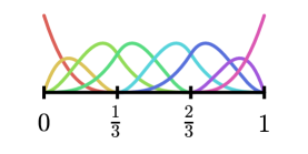
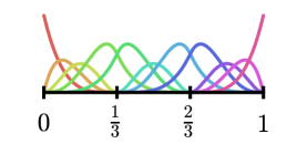
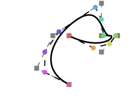
It can be seen that the elevated knot vector is obtained by increasing the multiplicity of each knot in the original knot vector by one. The basis functions generated by these knot vectors are shown above the curves and the basis functions are colored to match the associated control points. The extraction operator on the second element in the source mesh is
| (100) |
The Bernstein degree elevation matrix to elevate from degree 3 to degree 4 is given by Eq. 95 as
| (101) |
The extraction operator on second element in the target mesh defined by Eq. 99 is
| (102) |
and so the associated reconstruction operator is
| (103) |
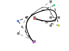
These are the matrices required for Eq. 97. The result of using these matrices and the appropriate matrices for the other elements in the mesh to elevate the original curve in the lower center of Fig. 19 is shown on the lower right of the same figure. The original curve and control points are shown in gray on the right for reference. It can be seen that the elevated curve exactly represents the original curve and that the new control points lie on the lines connecting the original control points.
| degree reduced | original curve | degree elevated |
|---|---|---|
 |
 |
 |
 |
 |
 |
Degree reduction or -coarsening can be viewed as Bézier projection from one spline space to another spline space of lower polynomial degree in at least one dimension. The projection is approximate. For tensor-product splines -coarsening is accomplished by decrementing the multiplicity of each knot and the polynomial degree in any dimension that is to be reduced. Next, the Bézier element extraction operators for the source mesh, the element reconstruction operators for the target mesh, and the transformation matrix between the Bernstein bases on the source and target meshes are computed.
The transformation matrix that provides the best approximation of the Bernstein basis of degree by the basis of degree is given by the right pseudoinverse of the matrix defined by Eq. 95
| (104) |
This is due to the fact that the best projection for polynomial degree reduction is given by the best Euclidean approximation of the the Bézier coefficients [66, 70]. In other words, for degree reduction of Bernstein polynomials, projection of the functions reduces to projection of the function coefficients. The multivariate transformation matrix is given by the Kronecker product of the one-dimensional matrices
| (105) |
where .
Algorithm 4.5.
Degree reduction of a B-spline or NURBS (-coarsening)
-
1.
Create the target mesh by decrementing the degree and knot multiplicity in each parametric direction that is to be reduced.
-
2.
Perform the Bézier projection
(106) -
3.
Smooth the result
(107)
An example of this process is given in Fig. 19. The degree-reduced basis is defined by the knot vector
The original basis is again defined by Eq. 98 and so the exraction operator on the second element of the source mesh is given by Eq. 100. The extraction operator for the second element in the target mesh is
| (108) |
and so the associated reconstruction operator is
| (109) |
The degree reduction operator from degree 3 to degree 2 is
| (110) |
The averaging weights for the target basis are the same as for the example illustrated in Fig. 7. The result of applying Algorithm 4.5 to degree reduce the curve in the lower center of Fig. 19 is shown on the lower left of the same figure and the original curve is shown in gray for reference; it is apparent that the degree reduced curve is only an approximation to the original curve. This is in contrast to the elevated case in which the curve was preserved exactly.
4.3 -adaptivity of T-splines
Degree elevation of a T-spline is achieved by increasing the degree and multiplicity of each edge in each elevation direction by one and propagating T-junctions through any new repeated edges. To ensure nestedness of degree elevated T-splines requires that the extended source and target T-meshes are nested and analysis-suitable. This is a mild generalization of Theorem 2.5.
Consider the even-to-odd degree elevation example shown in Fig. 20. A representative source mesh is shown in Fig. 20a. The degree and multiplicity of each edge in each elevation direction is increased by one and T-junctions are propagated through any new repeated edges. This process produces the target mesh shown in Fig. 20b. It can be easily verified that the extended T-meshes are nested. This ensures that the quadratic T-spline basis function, anchored at the orange diamond in Fig. 20a, can be exactly represented in the degree elevated T-mesh by the four cubic functions anchored at the blue diamonds in Fig. 20b.
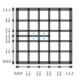
Now consider the odd-to-even degree elevation example shown in Fig. 21. A representative source mesh is shown in Fig. 21a. Again, the degree and multiplicity of each edge in each elevation direction is increased by one and T-junctions are propagated through any new repeated edges. However, in this case the extended T-meshes are not nested due to the repeated vertical edges at . Inspection of the mesh shown in Fig. 21b reveals that the nine quadratic functions, anchored at the blue diamonds in Fig. 21b, needed to represent the linear function anchored at the orange diamond in Fig. 21a, are not reproduced by the refined T-mesh in Fig. 21b. In this case, each T-junction must be extended across a single parametric element and through the repeated edges on the opposite side as shown in Fig. 21c.
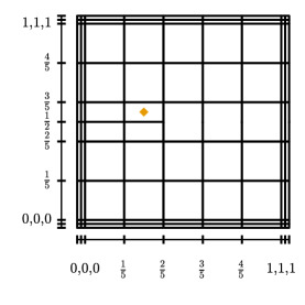 |
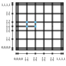 |
| (a) original mesh () | (b) elevated mesh () |
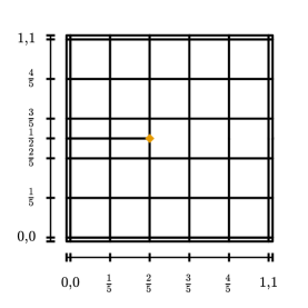 |
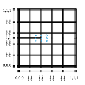 |
| (a) original mesh () | (b) elevated mesh () |
 |
|
| (c) extended elevated mesh () |
Algorithm 4.6.
Degree elevation of an analysis-suitable T-spline (-refinement)
-
1.
Create the target mesh by incrementing the degree and multiplicity of all T-mesh edges in each parametric direction that is to be elevated.
-
2.
Extend all T-junctions through any repeated edges.
-
3.
Modify T-junctions so that and is analysis-suitable.
-
4.
Continue from step 2 of Algorithm 4.4.
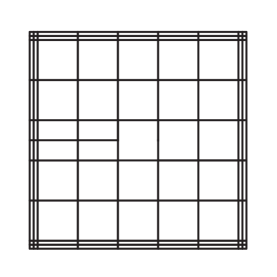
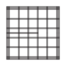
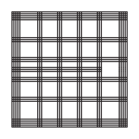
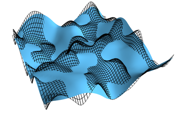
An example of T-spline degree elevation is shown in Fig. 22. The original T-mesh for a T-spline of degree 3 in each direction is shown in the upper center of the figure. Repeated knots are indicated by closely spaced edges. A random surface is generated by assigning a uniformly distributed random value between and to the elevation values of the control points that generate a linearly parameterized surface. This random surface is shown in the lower center. The degree elevation algorithm for ASTS is applied to the original mesh to obtain the degree-elevated mesh shown in the upper right. The result of applying the Bézier projection algorithm to compute the elevated surface shown in the lower right. The original surface is shown as a wireframe for comparison while the elevated surface is blue. It can be seen that the elevated surface coincides exactly with the original surface.
| degree-reduced T-mesh | original T-mesh | degree-elevated T-mesh |
 |
 |
 |
 |
 |
 |
| degree-reduced surface | original surface | degree-elevated surface |
Algorithm 4.7.
Degree reduction of an analysis-suitable T-spline (-coarsening)
-
1.
Create the target mesh by decrementing the degree and multiplicity of all T-mesh edges in each parametric direction that is to be reduced.
-
2.
Modify T-junctions so that and is analysis-suitable.
-
3.
Continue from step 2 of Algorithm 4.5.
An example of T-spline degree reduction is shown in Fig. 22. The degree reduction algorithm is applied to the original T-mesh in the upper center to obtain the reduced T-mesh shown on the upper left. The result of applying the Bézier projection algorithm to compute the reduced surface is shown in the lower left. The original surface is shown as a wireframe for comparison while the reduced surface is blue. It can be seen that while the reduced surface has an overall shape similar to the original surface, as expected, the two surfaces do not match.
Remark 4.8.
Due to T-junction extension in degree elevation and T-junction retraction in degree reduction the number of Bézier elements defined by the source and target T-meshes may be different. In that case, Algorithm 4.1 may be required to compute the projection.
4.4 -adaptivity of B-splines and NURBS
Basis roughening or -refinement is achieved by increasing the multiplicity of some or all of the knots. Basis smoothing or -coarsening is achieved by decreasing the multiplicity of some or all of the knots.
Algorithm 4.9.
Roughening of a NURBS or B-spline (-refinement)
-
1.
Create the target mesh by incrementing the knot multiplicity of some of the knots in each parametric direction that is to be roughened.
-
2.
Perform the Bézier projection
(111)
Because the spline spaces are nested the weighted averaging step is not required.
Algorithm 4.10.
Smoothing of a NURBS or B-spline (-coarsening)
-
1.
Create the target mesh be decrementing the knot multiplicity of some of the knots in each parametric direction that is to be smoothed.
-
2.
Perform the Bézier projection using Eq. 111.
-
3.
Smooth the result
(112)
| smoothed | original curve | roughened |
|---|---|---|
 |
 |
 |
 |
 |
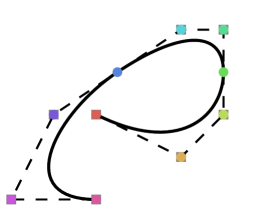 |
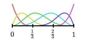
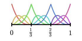
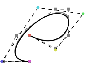
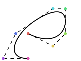
Basis roughening and coarsening for a one-dimensional B-spline curve are illustrated in Fig. 23. We begin with a cubic B-spline basis defined by the knot vector
| (113) |
The basis is shown in the upper center of Fig. 23. The extraction operator on the second element defined by this knot vector is the same as for the degree elvation example given previously in Eq. 100 A set of control points is chosen to define the curve shown in the lower center of the figure. A refined or roughened basis is defined by the knot vector
| (114) |
Because the knot multiplicity is equal to the polynomial degree, the extraction and reconstruction operators defined by this knot vector are identity matrices of size .
A smoothed basis is defined by the knot vector
| (115) |
The element extraction and reconstruction operators for the second element in the smoothed mesh are
| (116) |
and
| (117) |
The roughened and smoothed bases are shown in the upper right and left of Fig. 23 and the projection of the original curve onto the new basis is shown below each. It is apparent that the refined basis exactly represents the original curve (shown in gray for comparison) and that the number of control points has been increased (indicating the increased dimension of the roughened spline space). In contrast, the coarsened basis cannot fully represent the original curve because of the increased continuity and the reduced size of the basis.
4.5 -adaptivity of T-splines
Roughening or -refinement of a T-spline is achieved by increasing the multiplicity of each edge in each roughening direction by one and propagating T-junctions through any new repeated edges. To ensure nestedness of roughened or -refined T-splines requires that the extended source and target T-meshes are nested and analysis-suitable as described in Theorem 2.5.
Algorithm 4.11.
Roughening of a T-spline (-refinement)
-
1.
Create the target mesh by incrementing the multiplicity of any edges that are to be roughened.
-
2.
Extend all T-junctions through any repeated edges.
-
3.
Modify T-junctions so that and is analysis-suitable.
-
4.
Continue from step 2 of Algorithm 4.9
Smoothing of a T-spline is the opposite of roughening.
Algorithm 4.12.
Smoothing of a T-spline (-coarsening)
-
1.
Create the target mesh by decrementing the multiplicity of any edges that are to be smoothed.
-
2.
Modify T-junctions so that and is analysis-suitable.
-
3.
Continue from step 2 of Algorithm 4.10.
Examples of T-spline roughening and smoothing are shown in Fig. 24. The same random surface used for T-spline elevation and reduction is used.
| smoothed | original surface | roughened |
|---|---|---|
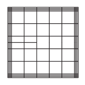 |
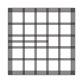 |
 |
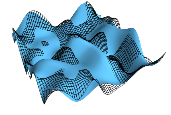 |
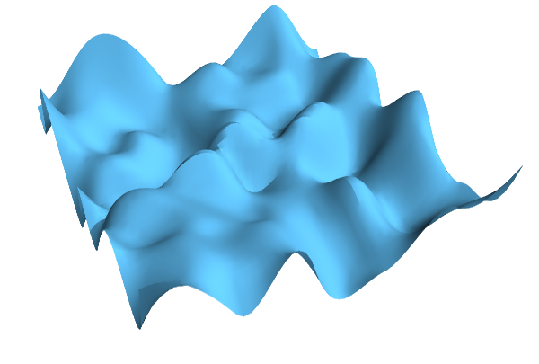 |
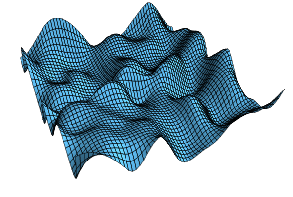 |
4.6 -adaptivity of B-splines and NURBS
Subdivision or -refinement is achieved by subdividing a set of knot intervals or elements with non-zero parametric length (area/volume).
Algorithm 4.13.
Subdivision for a B-spline or NURBS (-refinement)
-
1.
Create the target mesh by subdividing knot intevals with non-zero parametric length.
-
2.
Perform the Bézier projection in Algorithm 4.1.
Because the spline spaces are nested the weighted averaging step is not required.
To illustrate Algorithm 4.13 and in particular the application of Algorithm 4.1 we derive global refinement of a univariate B-spline using Bézier projection. The knot vector is
| (118) |
The quadratic basis is shown in the upper center of Fig. 25. A new knot vector is constructed by dividing every nonzero knot interval in half to obtain
| (119) |
The refined basis is shown on the upper right of Fig. 25. The element extraction operators for both the source and target meshes can be be computed using the methods given by Borden et al. [12] and Scott et al. [80]. All that remains in order to use Algorithm 4.1 is the computation of . As stated in Algorithm 4.1, the transformation operator is found by converting the bounds of the small (target) element to the local coordinates of the large (source) element and then using Eq. 12. We follow the standard finite-element convention that the local coordinate system of an element is the domain . For each element in the source mesh, we must project onto two new elements, one bounded by and in the local coordinate system of the source element and the other bounded by and . There is a distinct transformation operator associated with each of the new elements which we denote for the left subelement (the subdomain ) and for the right subelement (the subdomain ). The boundaries of each subelement are used for and while and are used for and in Eq. 12 to obtain
| (120) |
The extraction operator for the first element in the source mesh (corresponding to the interval ) is
| (121) |
The element extraction operators for the first two elements of the target mesh (corresponding to the intervals and ) are
| (123) | ||||
| (124) |
The reconstruction operators for these elements are
| (125) | ||||
| (126) |
The control points associated with the first interval in the target mesh are given by
| (127) |
where and and the control points for the second interval are given by
| (128) |
where . Because the source space is a subspace of the target space, the values computed for and will be the same for both of the target elements. The results of carrying the projection process out for the control points that define the curve in the lower center of Fig. 25 are shown on the right of the same figure.
| coarsened | original curve | refined |
|---|---|---|
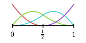 |
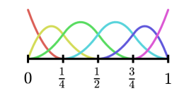 |
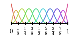 |
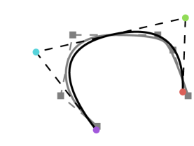 |
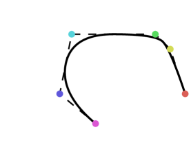 |
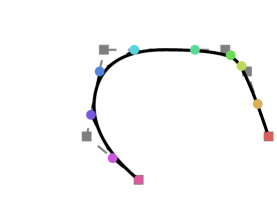 |
Merging or -coarsening is achieved by removing unique knots to combine two or more knot intervals into a single interval.
Algorithm 4.14.
Merging for a B-spline or NURBS (-coarsening)
-
1.
Create the target mesh by removing knots.
-
2.
Perform the Bézier projection in Algorithm 4.3.
-
3.
Smooth the result
(129)
To illustrate Algorithm 4.14 we remove knots and from to obtain
| (130) |
The basis defined by this knot vector is shown in the upper left of Fig. 25. The element extraction operators for the first two elements in the source mesh (knot intervals and ) are
| (131) | ||||
| (132) |
and the element extraction and reconstruction operators for the first element of the target mesh (knot interval ) that the two source elements are projected onto are
| (133) | ||||
| (134) |
The matrices used to transform the Bézier coefficients of the source elements onto the target element are computed by converting the lower and upper bounds of the target element into the local coordinates of the source elements. For this case, the bounds of the target element map to and on the first source element and and on the second source element. These values for the upper and lower bounds are used as values for and in Eq. 13 while and to obtain
| (135) | ||||
| (136) |
Note that is in fact the inverse of the matrix defined in the previous example of -refinement and is the inverse of . Each of the source elements covers half of the target element and so the weight for the relative contribution of each element to the final control points is . Finally, the Gramian matrix for the Bernstein basis of degree 2 is
| (137) |
The expression for the points points on given by Algorithm 4.3 for this problem is
| (138) |
where and . The result obtained by completing this process for the remaining elements and computing the weighted average of the resulting control points on each element in the target mesh is shown in the lower left of Fig. 25. It can be seen that the coarsened basis cannot fully capture the original curve (shown in gray for comparison).
4.7 -adaptivity of T-splines
Subdivision or -refinement and merging or -coarsening of a T-spline is achieved by subdividing or merging Bézier elements in the T-mesh.
Algorithm 4.15.
Subdivision for a T-spline (-refinement)
-
1.
Create the target mesh by adding edges to the T-mesh.
-
2.
Extend T-junctions so that and is analysis-suitable.
-
3.
Perform the Bézier projection in Algorithm 4.1.
Because the spline spaces are nested the weighted averaging step is not required.
Algorithm 4.16.
Merging for a T-spline (-coarsening)
-
1.
Create the target mesh by removing edges from the T-mesh.
-
2.
Modify T-junctions so that and is analysis-suitable.
-
3.
Continue from step 2 of Algorithm 4.14.
We present simple examples of T-spline subdivision and merging in Fig. 26. The original T-mesh is shown in the upper center of the figure. A randomly generated surface is shown in the lower center of Fig. 26. The refined T-mesh is produced by adding edges in the upper left and lower right corners of the original T-mesh to obtain the T-mesh shown in the upper right of the figure. New control point positions are computed by Bézier projection. The original and refined surfaces are compared in the lower right of the figure using the same convention to distinguish between the two as in the previous two T-spline examples (Figs. 22 and 24). It can be seen that the refined surface coincides exactly with the original surface. The coarsened mesh is shown in the upper left of the figure. The coarsened mesh is obtained from the original T-mesh by removing edges from 3 cells in the upper and lower left corners of the mesh. The new control point positions are computed by Bézier projection. The original and coarsened surfaces are compared in the lower left of Fig. 26. It can be seen that the coarsened surface only approximates the original surface.
| coarsened T-mesh | original T-mesh | refined T-mesh |
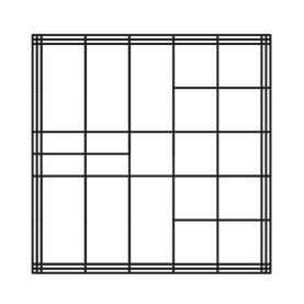 |
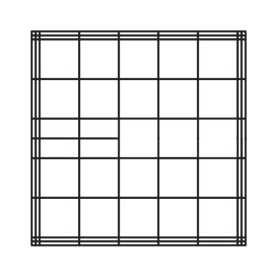 |
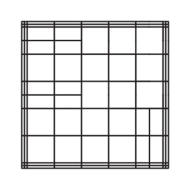 |
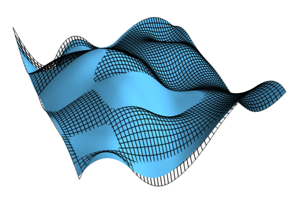 |
 |
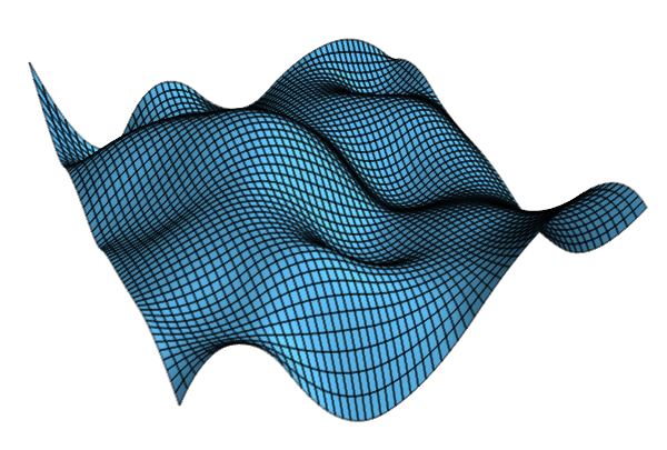 |
| coarsened surface | original surface | refined surface |
4.8 -adaptivity of B-splines, NURBS, and T-splines
Reparameterization or -adaptivity in this paper refers to the process of moving knots or T-mesh edges. This can be used to adjust the relative size of elements and hence the resolution of the mesh while leaving the number of degrees of freedom unchanged. Reparametrization does not generally produce nested spaces. Reparameterization requires combined use of Algorithms 4.1 and 4.3.
Algorithm 4.17.
Reparameterization of B-splines, NURBS, and T-splines (-adaptivity)
-
1.
Create the target mesh by repositioning knots or edges.
-
2.
Compute a target-to-source element map by enumerating all source elements that must be projected onto each target element.
-
3.
For each element in the target mesh if the number of elements that are to be projected onto the element is greater than one, use Algorithm 4.3, otherwise use Algorithm 4.1.
-
4.
Smooth the result
(139)
An example of reparameterization is given in Fig. 27 for a B-spline curve. The knot vector for the source mesh is
| (140) |
and the spline basis defined by this knot vector is shown in the upper center of Fig. 27. The reparameterized knot vector is chosen as
| (141) |
and the associated basis is shown in the upper right of Fig. 27. The target-to-source element map is
| (142) |
This means that elements 1 and 2 in the source mesh must be projected onto element 1 in the target mesh and element 2 in the source mesh must be projected onto element 2 in the target mesh. The element extraction operators defined by the source mesh are
| (143) | ||||
| (144) |
The element extraction operators defined by the target mesh are
| (145) | ||||
| (146) |
The associated reconstruction operators are
| (147) | ||||
| (148) |
| left reparameterization | original curve | right reparameterization |
|---|---|---|
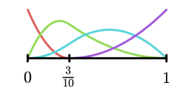 |
 |
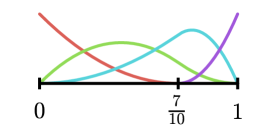 |
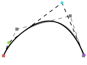 |
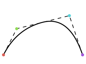 |
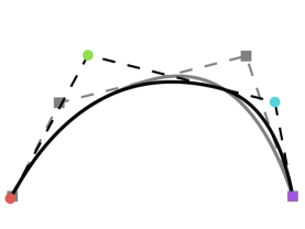 |
We begin with the projection of the control points associated with and on the source mesh onto the element on the target mesh. Algorithm 4.3 must be used because two elements are being projected onto one element. The transformation matrix that connects the Bernstein basis on to the basis on is found by converting the lower and upper bounds of to the local coordinates of to obtain and . Using these values with and in Eq. 13, the transformation matrix is
| (149) |
Because the spline segments over and must be projected onto it is necessary to find an intermediate representation of the segment from so that Algorithm 4.3 can be applied. The representation of the segment over the element defined by the intersection of and is found by multiplying the Bézier coefficients on by
| (150) |
This matrix is given by Eq. 12 with , , , . The transformation matrix to convert from the representation over to is given by Eq. 13 with and
| (151) |
The Bernstein basis is again of degree 2 and so the Gramian is given by Eq. 137. The element fractions are and . The set of control points associated with element is and the set of control points associated with element is . With this information, the control points on the target element are given by
| (152) |
The control points on element are found by projecting the control points from and so Algorithm 4.1 is appropriate. The transformation matrix is given by Eq. 12 with , , and the element boundaries of are converted to the local coordinates of to obtain and :
| (153) |
The control points on are given by
| (154) |
The weighted average of the control points on each element to obtain the global control points is now computed. The weights for the basis functions shown in the upper right of Fig. 27 for each element are
| (155) | ||||
| (156) |
The global control points are thus given by
The result of this process is illustrated for a simple curve in Fig. 27. The original curve and control points are shown in the lower center and the new curve, produced by the projection of the original control points onto the reparameterized basis, and control points are shown in the lower right. Since the spaces are not nested the two curves are not equal (the source curve is shown in gray on the lower right for comparison). The reparameterization produced by shifting the center knot to the left instead of to the right is shown on the left of Fig. 27 for comparison. Because the slope of the curve at the new knot location is better represented in the left-shifted basis than in the right-shifted basis, the new curve produced by projection onto the left-shifted basis more closely approximates the original curve than the right-shifted basis.
Two simple examples of reparameterization applied to a T-spline are shown in Fig. 28.
| left shifted T-mesh | original T-mesh | right shifted T-mesh |
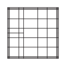 |
 |
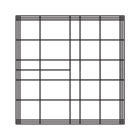 |
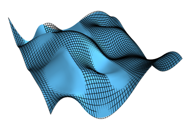 |
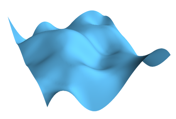 |
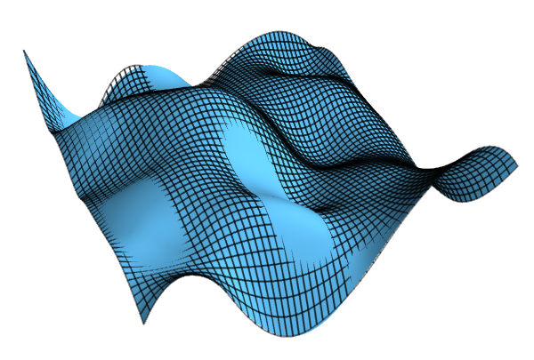 |
| left shifted surface | original surface | right shifted surface |
4.9 Combining -, -, -, and -refinement and coarsening
Refinement and coarsening by Bézier projection lends itself well to the successive application of different refinement and coarsening procedures. Once the control values have been converted to Bézier form each operation is accomplished by the application of the appropriate matrix. When applying multiple operations it is most efficient to convert to Bézier form, apply all necessary transformation matrices to the Bernstein coefficients, and then convert to spline form and, if necessary, apply the weighted averaging algorithm as the final processing step. If any of the operations are not exact then this approch avoids the accumulation of error associated with each weighted averaging step. The result will be identical if all of the operations are exact.
5 Summary and conclusions
We have presented Bezier projection as a unified approach to local projection, refinement, and coarsening of NURBS and T-splines. The approach employs a simple three-step procedure, namely, projection onto a local basis, conversion to a global basis, and smoothing using a weighting scheme. Moreover, the approach relies on the fundamental concept of Bezier extraction and the associated spline reconstruction developed here, resulting in an element-based formulation that may be easily implemented in existing finite element codes. Optimal convergence rates are proven, and a novel weighting scheme is presented that leads to dramatic improvements in accuracy over previous approaches. In fact, by comparing our Fig. 11 to Fig. 5 in Govindjee et al. [47], it can be seen that the methodology proposed here produces significantly better results. Several exemplary applications of Bezier projection are presented to illustrate the accuracy, robustness, and flexibility of the method.
In the event that data fitting or interpolation is desired, Bézier projection is easily modified to accomodate these cases. There are efficient and accurate methods for determining the Bernstein representation of a polynomial interpolating function [68, 69]. Once the Bernstein representation has been computed, the spline segment representation over each element can be computed using the element reconstruction operator and the weighted average is computed as before.
This procedure of computing a Bernstein representation, converting to a local spline representation, and then smoothing the result to obtain a smooth global spline representation or approximation provides a general tool for adapting methods developed for Bernstein polynomials into methods for splines. Indeed, the whole host of methods and techniques developed for Bernstein polynomials can be applied locally, converted to spline form and then a smoothed global spline approximation can be computed using the weighted averaging developed here. A retrospective overview of work on Bernstein polynomials is given by Farouki [40] and many interesting possibilities can be found there and in the references contained therein.
A unified framework was developed for quadrature-free degree elevation, degree reduction, knot insertion, knot removal, and reparameterization of B-splines, NURBS, and T-splines that requires only element-level information. We feel that Bézier projection provides the fundamental building blocks required for -adaptivity in isogeometric analysis.
Appendix A Optimal convergence of the Bézier projection operator
In this appendix, we prove that the Bézier projection operator presented in this paper exhibits optimal convergence rates. For the sake of brevity, we restrict our discussion to the one-dimensional setting. By using the methods presented in [4] and [26], one may extend our theory to the multi-dimensional, rational, and analysis-suitable T-spline settings. In what follows, denotes a univariate B-spline space consisting of -continuous piecewise polynomials of degree . We assume that the parametric space and physical space coincide, simplifying our exposition. We additionally employ the simplified notation to represent the Bézier projection operator wherein it is assumed that . Throughout this appendix, we exploit the notion of a Bézier element. We denote each Bézier element using index and the domain of each Bézier element using , and we define to be the set of all Bézier elements. We will also need the notion of a support extension. For a Bézier element , the support extension is the union of the supports of basis functions whose support intersects .
The first ingredient we need in proving optimal convergence of the Bézier projection operator is approximability. The following lemma states the local approximation properties of the spline space , and a proof of the lemma may be found in [4].
Lemma A.1.
Let and be integer indices with and . For each Bézier element , there exists an such that
| (A.1) |
where is the mesh size of element , is the support extension of element , and is a constant independent of but possibly dependent on the shape regularity of the mesh, polynomial degree, continuity, and the parameters and .
The next two ingredients we need in proving optimal convergence are idempotence and local stability. The following lemma states these properties for the Bézier projection operator. The proof of the lemma is rather involved, so we postpone the proof until later in the appendix.
Lemma A.2.
We have:
| (spline-preserving property) | (A.2) | |||||||||
| (local stability property) | (A.3) | |||||||||
where is a constant independent of but possibly dependent on the shape regularity of the mesh, polynomial degree, and continuity.
Using Lemmata A.1 and A.2 we can state the convergence properties of the Bézier projection operator.
Theorem A.3.
Let and be integer indices with and . For each Bézier element , the following inequality holds:
| (A.4) |
where is the mesh size of element , is the support extension of element , and is a constant independent of but possibly dependent on the shape regularity of the mesh, polynomial degree, continuity, and the parameters and .
Proof.
We now return to the proof of Lemma A.2. While the spline-preserving property holds trivially, the local stability property is more technical to establish. To proceed, we will need the results of the following two lemmata. The first lemma concerns the stability of the local Bézier element extraction operator and its inverse while the second concerns the stability of local -projection onto the Bernstein basis.
Lemma A.4.
For each Bézier element , the norm of the element extraction operator (and its inverse) is independent of the mesh size but possibly dependent on the shape regularity of the mesh, polynomial degree, and continuity.
Proof.
The lemma is a consequence of the fact that the element extraction operators for a given B-spline space are invariant under constant scalings of the domain . ∎
Lemma A.5.
For each Bézier element , the local Bernstein coefficient vector associated with the local -projection of a function onto the space of polynomials of degree satisfies the inequality
| (A.5) |
where is the mesh size of element and is a constant only dependent upon the polynomial degree .
Proof.
The vector of coefficients are defined through the equation:
where with
and with
In the above equation, is the standard affine map from the biunit interval onto element . Since , we have that
The last inequality above follows from Hölder’s inequality. Moreover, by scaling, we have that where is a constant only dependent upon the polynomial degree . The desired result immediately follows with . ∎
With the preceding two lemmata established, we are now in a position to complete the proof of Lemma A.2.
Proof of Lemma A.2.
The spline-preserving property holds trivially. Hence, it remains to prove the local stability property. Let and . We have that:
where is the index set of all B-spline basis functions whose support overlaps with element . For each , the weights satisfy and the vector of coefficients is defined by
where is the local Bernstein coefficient vector associated with the local -projection of onto element . The results of the previous two lemmas dictate that
where is the mesh size of element and is a constant which only depends on the polynomial degree , the continuity , and the shape regularity of the parametric mesh. Since the B-spline basis functions are positive and form a partition of unity, we consequently have that
over element where is a constant only dependent on the shape regularity of the mesh and is the support extension of element . Therefore:
Thus the local stability result holds with . ∎
References
- Autodesk [2012] Autodesk, 2012. Autodesk T-Splines Plug-in for Rhino user manual. Autodesk.
- Autodesk, Inc. [2014] Autodesk, Inc., 2014. Autodesk Fusion 360. Autodesk, Inc.
- Barrera et al. [2008] Barrera, D., Ibáñez, M., Sablonnière, P., Sbibih, D., 2008. Near-best univariate spline discrete quasi-interpolants on nonuniform partitions. Constructive Approximation 28 (3), 237–251.
- Bazilevs et al. [2006] Bazilevs, Y., Beirao de Veiga, L., Cottrell, J., Hughes, T. J. R., Sangalli, G., 2006. Isogeometric analysis: approximation, stability and error estimates for -refined meshes. Mathematical Models and Methods in Applied Sciences 16, 1031–1090.
- Bazilevs et al. [2010] Bazilevs, Y., Calo, V. M., Cottrell, J. A., Evans, J. A., Hughes, T. J. R., Lipton, S., Scott, M. A., Sederberg, T. W., 2010. Isogeometric analysis using T-splines. Computer Methods in Applied Mechanics and Engineering 199 (5-8), 229–263.
- Bazilevs et al. [2012] Bazilevs, Y., Hsu, M. C., Scott, M. A., 2012. Isogeometric fluid-structure interaction analysis with emphasis on non-matching discretizations, and with application to wind turbines. Computer Methods in Applied Mechanics and Engineering 249 - 252, 28 – 41.
- Beirão da Veiga et al. [2012] Beirão da Veiga, L., Buffa, A., Cho, D., Sangalli, G., 2012. Analysis-suitable T-splines are dual-compatible. Computer Methods in Applied Mechanics and Engineering 249 – 252, 42 – 51.
- Benson et al. [2010] Benson, D. J., Bazilevs, Y., De Luycker, E., Hsu, M. C., Scott, M. A., Hughes, T. J. R., Belytschko, T., 2010. A generalized finite element formulation for arbitrary basis functions: From isogeometric analysis to XFEM. International Journal for Numerical Methods in Engineering 83, 765–785.
- Berdinsky et al. [2014] Berdinsky, D., wan Kim, T., Bracco, C., Cho, D., Mourrain, B., Oh, M., Kiatpanichgij, S., 2014. Dimensions and bases of hierarchical tensor-product splines. Journal of Computational and Applied Mathematics 257, 86 – 104.
- Bézier [1966] Bézier, P., 1966. Définition numérique des courbes et surfaces I. Automatisme XI, 625–632.
- Bézier [1967] Bézier, P., 1967. Définition numérique des courbes et surfaces II. Automatisme XII, 17–21.
- Borden et al. [2011] Borden, M. J., Scott, M. A., Evans, J. A., Hughes, T. J. R., 2011. Isogeometric finite element data structures based on Bézier extraction of NURBS. International Journal for Numerical Methods in Engineering, 87, 15 – 47.
- Borden et al. [2012] Borden, M. J., Scott, M. A., Verhoosel, C. V., Landis, C. M., Hughes, T. J. R., 2012. A phase-field description of dynamic brittle fracture. Computer Methods in Applied Mechanics and Engineering 217, 77 – 95.
- Bracco et al. [2014] Bracco, C., Berdinsky, D., Cho, D., Oh, M., wan Kim, T., 2014. Trigonometric generalized T-splines. Computer Methods in Applied Mechanics and Engineering 268, 540 – 556.
- Bressan [2013] Bressan, A., 2013. Some properties of LR-splines. Computer Aided Geometric Design 30 (8), 778 – 794.
- Buffa et al. [2014] Buffa, A., Sangalli, G., Vázquez, R., 2014. Isogeometric methods for computational electromagnetics: B-spline and T-spline discretizations. Journal of Computational Physics 257, Part B, 1291 – 1320.
- Burkhart et al. [2010] Burkhart, D., Hamann, B., Umlauf, G., 2010. Isogeometric finite element analysis based on Catmull-Clark subdivision solids. In: Computer Graphics Forum. Vol. 29. Wiley Online Library, pp. 1575–1584.
- Catmull and Clark [1978] Catmull, E., Clark, J., 1978. Recursively generated B-spline surfaces on arbitrary topological meshes. Computer Aided Design 10, 350–355.
- Cirak et al. [2000] Cirak, F., Ortiz, M., Schrder, P., 2000. Subdivision surfaces: A new paradigm for thin shell analysis. International Journal for Numerical Methods in Engineering 47, 2039–2072.
- Cohen et al. [1980] Cohen, E., Lyche, T., Riesenfeld, R., 1980. Discrete B-splines and subdivision techniques in computer-aided geometric design and computer graphics. Computer Graphics and Image Processing 14 (2), 87 – 111.
- Cohen et al. [2010] Cohen, E., Martin, T., Kirby, R. M., Lyche, T., Riesenfeld, R. F., 2010. Analysis-aware modeling: Understanding quality considerations in modeling for isogeometric analysis. Computer Methods in Applied Mechanics and Engineering 199 (5-8), 334–356.
- Constantini et al. [2010] Constantini, P., Manni, C., Pelosi, F., Sampoli, M. L., 2010. Quasi-interpolation in isogeometric analysis based on generalized B-splines. Computer Aided Geometric Design 27 (8), 656–668.
- Cottrell et al. [2009] Cottrell, J. A., Hughes, T. J. R., Bazilevs, Y., 2009. Isogeometric analysis: Toward Integration of CAD and FEA. Wiley, Chichester.
- Cottrell et al. [2007] Cottrell, J. A., Hughes, T. J. R., Reali, A., 2007. Studies of refinement and continuity in isogeometric analysis. Computer Methods in Applied Mechanics and Engineering 196, 4160–4183.
- Cottrell et al. [2006] Cottrell, J. A., Reali, A., Bazilevs, Y., Hughes, T. J. R., 2006. Isogeometric analysis of structural vibrations. Computer Methods in Applied Mechanics and Engineering 195, 5257–5296.
- da Veiga et al. [2013] da Veiga, L. B., Buffa, A., Sangalli, G., Vázquez, R., 2013. Analysis-suitable T-splines of arbitrary degree: definition, linear independence, and approximation properties. Mathematical Models and Methods in Applied Sciences 23 (11), 1979 – 2003.
- de Boor [1972] de Boor, C., 1972. On calculating with B-splines. Journal of Approximation Theory 6 (1), 50 – 62.
- de Boor [1990] de Boor, C., 1990. Quasiinterpolants and approximation power of multivariate splines. In: Dahmen, W., Gasca, M., Micchelli, C. (Eds.), Computation of Curves and Surfaces. Vol. 307 of NATO ASI Series. Springer Netherlands, pp. 313–345.
- de Boor and Fix [1973] de Boor, C., Fix, G., 1973. Spline approximation by quasiinterpolants. Journal of Approximation Theory 8 (1), 19 – 45.
- de Casteljau [1963] de Casteljau, P., 1963. Courbes et surfaces a poles. Tech. rep., A. Citroen.
- Deng et al. [2008] Deng, J., Chen, F., Li, X., Hu, C., Tong, W., Yang, Z., Feng, Y., 2008. Polynomial splines over hierarchical T-meshes. Graphical Models 74, 76–86.
- Dimitri et al. [2014] Dimitri, R., Lorenzis, L. D., Scott, M. A., Wriggers, P., Taylor, R., Zavarise, G., 2014. Isogeometric large deformation frictionless contact using T-splines. Computer methods in applied mechanics and engineering 269, 394 – 414.
- Doha et al. [2011] Doha, E., Bhrawy, A., Saker, M., 2011. Integrals of bernstein polynomials: An application for the solution of high even-order differential equations. Applied Mathematics Letters 24 (4), 559 – 565.
- Dokken et al. [2013] Dokken, T., Lyche, T., Pettersen, K. F., 2013. Polynomial splines over locally refined box-partitions. Computer Aided Geometric Design 30 (3), 331–356.
- Donea et al. [1982] Donea, J., Giuliani, S., Halleux, J. P., 1982. An arbitrary Lagrangian-Eulerian finite element method for transient dynamics fluid-structure interactions. Computer Methods in Applied Mechanics and Engineering 33, 689–723.
- Dörfel et al. [2009] Dörfel, M., Jüttler, B., Simeon, B., 2009. Adaptive isogeometric analysis by local h-refinement with T-splines. Computer Methods in Applied Mechanics and Engineering 199 (5–8), 264–275.
- Eck and Hadenfeld [1995] Eck, M., Hadenfeld, J., 1995. Knot removal for B-spline curves. Computer Aided Geometric Design 12 (3), 259 – 282.
- Evans et al. [2014] Evans, E. J., Scott, M. A., Li, X., Thomas, D. C., 2014. Hierarchical analysis-suitable T-splines: Formulation, Bézier extraction, and application as an adaptive basis for isogeometric analysis. arXiv:math.NA/1404.4346, submitted.
- Evans et al. [2009] Evans, J. A., Bazilevs, Y., Babuška, I., Hughes, T. J. R., 2009. n-widths, sup-infs, and optimality ratios for the k-version of the isogeometric finite element method. Computer Methods in Applied Mechanics and Engineering 198 (21-26), 1726–1741.
- Farouki [2012] Farouki, R. T., 2012. The Bernstein polynomial basis: A centennial retrospective. Computer Aided Geometric Design 29 (6), 379 – 419.
- Farouki and Neff [1990] Farouki, R. T., Neff, C. A., 1990. On the numerical condition of Bernstein-Bezier subdivision processes. Mathematics of Computation 55 (192), 637–647.
- Forsey and Bartels [1988] Forsey, D. R., Bartels, R. H., 1988. Hierarchical B-spline refinement. ACM SIGGRAPH Computer Graphics 22 (4), 205–212.
- Giannelli et al. [2012] Giannelli, C., Jüttler, B., Speleers, H., 2012. THB–splines: The truncated basis for hierarchical splines. Computer Aided Geometric Design 29 (7), 485 – 498.
- Giannelli et al. [2013] Giannelli, C., Jüttler, B., Speleers, H., 2013. Strongly stable bases for adaptively refined multilevel spline spaces. Advances in Computational Mathematics, 1–32.
- Ginnis et al. [2014] Ginnis, A. I., Kostas, K. V., Politis, C. G., Kaklis, P. D., Belibassakis, K. A., Gerostathis, T. P., Scott, M. A., Hughes, T. J. R., 2014. Isogeometric boundary-element analysis for the wave-resistance problem using T-splines. Computer Methods in Applied Mechanics and Engineering submitted.
- Goldman and Lyche [1993] Goldman, R., Lyche, T., 1993. Knot Insertion and Deletion Algorithms for B-Spline Curves and Surfaces. Society for Industrial and Applied Mathematics.
- Govindjee et al. [2012] Govindjee, S., Strain, J., Mitchell, T. J., Taylor, R. L., 2012. Convergence of an efficient local least-squares fitting method for bases with compact support. Computer Methods in Applied Mechanics and Engineering 213-216, 84–92.
- Grinspun et al. [2002] Grinspun, E., Krysl, P., Schröder, P., 2002. CHARMS: a simple framework for adaptive simulation. ACM Transactions on Graphics 21 (3), 281–290.
- Hosseini et al. [2014] Hosseini, S., Remmers, J. J., Verhoosel, C. V., de Borst, R., 2014. An isogeometric continuum shell element for non-linear analysis. Computer Methods in Applied Mechanics and Engineering 271, 1 – 22.
- Huang et al. [2005] Huang, Q.-X., Hu, S.-M., Martin, R. R., 2005. Fast degree elevation and knot insertion for B-spline curves. Computer Aided Geometric Design 22 (2), 183 – 197.
- Hughes et al. [2005] Hughes, T. J. R., Cottrell, J. A., Bazilevs, Y., 2005. Isogeometric analysis: CAD, finite elements, NURBS, exact geometry, and mesh refinement. Computer Methods in Applied Mechanics and Engineering 194, 4135–4195.
- Hughes et al. [2014] Hughes, T. J. R., Evans, J. A., Reali, A., 2014. Finite element and NURBS approximations of eigenvalue, boundary-value, and initial-value problems. Computer Methods in Applied Mechanics and Engineering 272, 290 – 320.
- Jaxon and Qian [2014] Jaxon, N., Qian, X., 2014. Isogeometric analysis on triangulations. Computer-Aided Design 46, 45 – 57.
- Johnson and Tezduyar [1994] Johnson, A. A., Tezduyar, T. E., 1994. Mesh update strategies in parallel finite element computations of flow problems with moving boundaries and interfaces. Computer Methods in Applied Mechanics and Engineering 119, 73–94.
- Jüttler [1998] Jüttler, B., 1998. The dual basis functions for the bernstein polynomials. Advances in Computational Mathematics 8 (4), 345–352.
- Kang et al. [2013] Kang, H., Chen, F., Deng, J., 2013. Modified T-splines. Computer Aided Geometric Design 30 (9), 827 – 843.
- Kiss et al. [2014] Kiss, G., Giannelli, C., Jüttler, B., 2014. Algorithms and data structures for truncated hierarchical B-splines. In: Floater, M., Lyche, T., Mazure, M.-L., Mørken, K., Schumaker, L. (Eds.), Mathematical Methods for Curves and Surfaces. Vol. 8177 of Lecture Notes in Computer Science. Springer Berlin Heidelberg, pp. 304–323.
- Lee et al. [2000] Lee, B.-G., Lyche, T., Mørken, K., 2000. Some examples of quasi-interpolants constructed from local spline projectors. In: In Mathematical Methods in CAGD: Oslo 2000, Vanderbilt. University Press, pp. 243–252.
- Li et al. [2006] Li, X., Deng, J., Chen, F., 2006. The dimension of spline spaces over 3d hierarchical T-meshes. Journal of Information and Computational Science 3, 487–501.
- Li et al. [2007] Li, X., Deng, J., Chen, F., 2007. Surface modeling with polynomial splines over hierarchical T-meshes. The Visual Computer 23, 1027–1033.
- Li et al. [2010] Li, X., Deng, J., Chen, F., 2010. Polynomial splines over general T-meshes. The Visual Computer 26, 277–286.
- Li and Scott [2014] Li, X., Scott, M. A., 2014. Analysis-suitable T-splines: characterization, refineability, and approximation. Mathematical Models and Methods in Applied Science 24 (06), 1141–1164.
- Li et al. [2012] Li, X., Zheng, J., Sederberg, T. W., Hughes, T. J. R., Scott, M. A., 2012. On linear independence of T-spline blending functions. Computer Aided Geometric Design 29, 63 – 76.
- Liu et al. [2014] Liu, L., Zhang, Y., Hughes, T. J. R., Scott, M. A., Sederberg, T. W., 2014. Volumetric T-spline construction using boolean operations. In: Sarrate, J., Staten, M. (Eds.), Proceedings of the 22nd International Meshing Roundtable. Springer International Publishing, pp. 405–424.
- Loop [1987] Loop, C., 1987. Smooth subdivision surfaces based on triangles. Master’s thesis, University of Utah.
- Lutterkort et al. [1999] Lutterkort, D., Peters, J., Reif, U., 1999. Polynomial degree reduction in the L2-norm equals best Euclidean approximation of Bezier coefficients. Computer Aided Geometric Design 16 (7), 607 – 612.
- Manni et al. [2011] Manni, C., Pelosi, F., Sampoli, M. L., 2011. Generalized B-splines as a tool in isogeometric analysis. Computer Methods in Applied Mechanics and Engineering 200 (5–8), 867 – 881.
- Marco and Martínez [2007] Marco, A., Martínez, J.-J., 2007. A fast and accurate algorithm for solving Bernstein-Vandermonde linear systems. Linear Algebra and its Applications 422 (23), 616 – 628.
- Marco and Martínez [2010] Marco, A., Martínez, J.-J., 2010. Polynomial least squares fitting in the Bernstein basis. Linear Algebra and its Applications 433 (7), 1254 – 1264.
- Peters and Reif [2000] Peters, J., Reif, U., 2000. Least squares approximation of Bezier coefficients provides best degree reduction in the L2-norm. Journal of Approximation Theory 104 (1), 90 – 97.
-
Piegl [1991]
Piegl, L., Jan. 1991. On NURBS: A survey. IEEE Comput. Graph. Appl. 11 (1),
55–71.
URL http://dx.doi.org/10.1109/38.67702 - Piegl and Tiller [1997] Piegl, L., Tiller, W., 1997. The NURBS Book. Springer-Verlag, New York.
- Prautzsch [1984] Prautzsch, H., 1984. Degree elevation of B-spline curves. Computer Aided Geometric Design 1 (2), 193 – 198.
- Riesenfeld [1973] Riesenfeld, R. F., 1973. Applications of B-spline approximation to geometric problems of computer-aided design. Ph.D. thesis, Syracuse University, Syracuse, NY, USA.
- Sablonnière [2005] Sablonnière, P., 2005. Recent progress on univariate and multivariate polynomial and spline quasi-interpolants. In: Mache, D. H., Szabados, J., Bruin, M. G. (Eds.), Trends and Applications in Constructive Approximation. Vol. 151 of ISNM International Series of Numerical Mathematics. Birkhauser Basel, pp. 229–245.
- Schillinger et al. [2012] Schillinger, D., Dedé, L., Scott, M. A., Evans, J. A., Borden, M. J., Rank, E., Hughes, T. J. R., 2012. An isogeometric design-through-analysis methodology based on adaptive hierarchical refinement of NURBS, immersed boundary methods, and T-spline CAD surfaces. Computer Methods in Applied Mechanics and Engineering 249 – 252, 116 – 150.
- Schillinger et al. [2013] Schillinger, D., Evans, J. A., Reali, A., Scott, M. A., Hughes, T. J. R., 2013. Isogeometric collocation: Cost comparison with Galerkin methods and extension to adaptive hierarchical NURBS discretizations. Computer Methods in Applied Mechanics and Engineering 267, 170 – 232.
- Schmidt et al. [2012] Schmidt, R., Wüchner, R., Bletzinger, K.-U., 2012. Isogeometric analysis of trimmed NURBS geometries. Computer Methods in Applied Mechanics and Engineering 241–244, 93 – 111.
- Scott [2011] Scott, M. A., 2011. T-splines as a Design-Through-Analysis technology. Ph.D. thesis, The University of Texas at Austin.
- Scott et al. [2011] Scott, M. A., Borden, M. J., Verhoosel, C. V., Sederberg, T. W., Hughes, T. J. R., 2011. Isogeometric Finite Element Data Structures based on Bézier Extraction of T-splines. International Journal for Numerical Methods in Engineering, 88, 126 – 156.
- Scott et al. [2012] Scott, M. A., Li, X., Sederberg, T. W., Hughes, T. J. R., 2012. Local refinement of analysis-suitable T-splines. Computer Methods in Applied Mechanics and Engineering 213, 206 – 222.
- Scott et al. [2013] Scott, M. A., Simpson, R. N., Evans, J. A., Lipton, S., Bordas, S. P. A., Hughes, T. J. R., Sederberg, T. W., 2013. Isogeometric boundary element analysis using unstructured T-splines. Computer Methods in Applied Mechanics and Engineering 254, 197 – 221.
- Scott et al. [2014] Scott, M. A., Thomas, D. C., Evans, E. J., 2014. Isogeometric spline forests. Computer Methods in Applied Mechanics and Engineering 269, 222 – 264.
- Sederberg et al. [2004] Sederberg, T. W., Cardon, D. L., Finnigan, G. T., North, N. S., Zheng, J., Lyche, T., August 2004. T-spline simplification and local refinement. ACM Trans. Graph. 23, 276–283.
- Sederberg et al. [2003] Sederberg, T. W., Zheng, J., Bakenov, A., Nasri, A., July 2003. T-splines and T-NURCCs. ACM Trans. Graph. 22, 477–484.
- Simpson et al. [2014] Simpson, R. N., Scott, M. A., Taus, M., Thomas, D. C., Lian, H., 2014. Acoustic isogeometric boundary element analysis. Computer Methods in Applied Mechanics and Engineering 269, 265–290.
- Speleers et al. [2013] Speleers, H., Manni, C., Pelosi, F., 2013. From NURBS to NURPS geometries. Computer Methods in Applied Mechanics and Engineering 255, 238–254.
- Speleers et al. [2012] Speleers, H., Manni, C., Pelosi, F., Sampoli, M. L., 2012. Isogeometric analysis with Powell–Sabin splines for advection–diffusion–reaction problems. Computer Methods in Applied Mechanics and Engineering 221, 132–148.
- Szafnicki [2005] Szafnicki, B., 2005. On the degree elevation of Bernstein polynomial representation. Journal of Computational and Applied Mathematics 180 (2), 443 – 459.
- Verhoosel et al. [2011a] Verhoosel, C. V., Scott, M. A., de Borst, R., Hughes, T. J. R., 2011a. An isogeometric approach to cohesive zone modeling. International Journal for Numerical Methods in Engineering, 87, 336 – 360.
- Verhoosel et al. [2011b] Verhoosel, C. V., Scott, M. A., Hughes, T. J. R., de Borst, R., 2011b. An isogeometric analysis approach to gradient damage models. International Journal for Numerical Methods in Engineering, 86, 115–134.
- Versprille [1975] Versprille, K. J., 1975. Computer-aided design applications of the rational B-spline approximation form. Ph.D. thesis, Syracuse University, Syracuse, NY, USA, aAI7607690.
- Vuong et al. [2011] Vuong, A., Giannelli, C., Jüttler, B., Simeon, B., 2011. A hierarchical approach to adaptive local refinement in isogeometric analysis. Computer Methods in Applied Mechanics and Engineering 200 (49 – 52), 3554 – 3567.
- Wall et al. [2008] Wall, W. A., Frenzel, M. A., Cyron, C., 2008. Isogeometric structural shape optimization. Computer Methods in Applied Mechanics and Engineering 197, 2976–2988.
- Wang et al. [2011] Wang, W., Zhang, Y., Scott, M. A., Hughes, T. J. R., 2011. Converting an unstructured quadrilateral mesh to a standard T-spline surface. Computational Mechanics, 48, 477 – 498.