Exploring Theory Space with Monte Carlo Reweighting

Abstract

Theories of new physics often involve a large number of unknown parameters which need to be scanned. Additionally, a putative signal in a particular channel may be due to a variety of distinct models of new physics. This makes experimental attempts to constrain the parameter space of motivated new physics models with a high degree of generality quite challenging. We describe how the reweighting of events may allow this challenge to be met, as fully simulated Monte Carlo samples generated for arbitrary benchmark models can be effectively re-used. In particular, we suggest procedures that allow more efficient collaboration between theorists and experimentalists in exploring large theory parameter spaces in a rigorous way at the LHC.

1 Introduction

Monte Carlo (MC) simulation is an essential and ubiquitous tool in particle physics Cowan ; Nason ; Beringer:1900zz ; Buckley:2011ms . For realistic studies, such simulation generally includes the modeling of the detector response as well as the underlying physical process. While theoretical studies generally require only “fast” detector simulation, such as that performed by PGS PGS4 or Delphes deFavereau:2013fsa , the modeling of the detector response to a given physics event at the experimental level, using frameworks such as GEANT Agostinelli:2002hh , is necessarily a time-consuming and computationally expensive process.

The challenge of accommodating the current lack of direct evidence for new physics within frameworks that address the limitations of the Standard Model (SM) leads to models with many parameters, such as the general gauge mediation Giudice:1998bp ; Carpenter:2008wi ; Intriligator:2008fr ; Meade:2008wd ; Carpenter:2008he ; Buican:2008ws ; Craig:2013wga and pMSSM Berger:2008cq ; Cotta:2009zu ; AbdusSalam:2009qd ; Sekmen:2011cz ; Arbey:2011un ; CMS:2013rda frameworks in low-energy Supersymmetry (SUSY)Martin:1997ns ; Drees:2004jm ; Baer:2006rs ; Dine:2007zp . Even when no particularly compelling model of Beyond the SM (BSM) physics exists for a given process, it may be useful to parameterize potential deviations from the SM using an effective theory Wilson:1973jj ; Georgi:1990um ; Georgi:1994qn ; Kaplan:1995uv ; Manohar:1996cq ; D'Ambrosio:2002ex ; Rothstein:2003mp ; Rajaraman:2011wf , which may involve many operators and hence many parameters.

In addition to the situations above which involve many continuous parameters, there are also issues with discrete parameters; in particular there can be many choices for the spin assignments for particles in a given event topology. A well-known example of this is the fact that most if not all SUSY topologies are also produced in models of Universal Extra Dimensions (UED) Appelquist:2000nn ; Cheng:2002ab . It is therefore desirable to study, at the very least, the UED counterparts of SUSY signal benchmark points.

Clearly experimentalists at the CERN Large Hadron Collider (LHC) and similar experiments are faced with an overwhelming multitude of theoretical models which could be searched for. To determine the properties of a given signal in the detector generally requires detector-level MC simulation (fullsim) of that signal, e.g., with GEANT, which is a time-consuming process, as noted above. To repeat this procedure for the myriad possibilities suggested by theorists is simply not possible.

Attempts have been made to solve this problem Cranmer:2010hk ; Rao:2012sx ; Drees:2013wra ; Papucci:2014rja , perhaps most notably by encouraging theorists to test the predictions of their models against suitably chosen experimental results (e.g., limits on cross-sections times branching fractions as a function of the mass spectrum). However, an actual discovery will still require the use of fullsim samples to obtain realistic distributions for the kinematic variables of interest (such as test statistics).

We propose and describe the following procedure for the experimental analysis of a large number of signal hypotheses:

1. Generate a large set of unweighted sample events at generator level, $\{G_{i}\}$ for a specific model and point in that model’s parameter space, which we term $(A,\bm{\alpha})$ (where $A$ describes the model and $\bm{\alpha}$ specifies a point in that model’s parameter space); a reasonable choice for the model, $A$, would be a simplified model ArkaniHamed:2007fw ; Alwall:2008ag ; Alves:2011wf ; ATLAS:2011lka ; Okawa:2011xg ; ATLAS:2011ffa ; Chatrchyan:2013sza .

2. Pass the generator-level events, $\{G_{i}\}$ through realistic detector simulation. Select desired events (“apply cuts”) to obtain a set of detector level events $\{D_{i}\}$. (Every generator-level event $G_{i}$ maps to some detector-level event, $D_{i}$, but not every detector-level event passes our cuts.)

3. Note that the cross section after acceptances and efficiencies, as well as the detector-level predictions for all distributions in signal hypothesis $(A,\bm{\alpha})$ can be obtained from the resulting event sample.

4. Choose some other model, $B$, and parameter space point, $\bm{\beta}$. Assign each detector-level event $D_{i}$ a weight $w(B,\bm{\beta},G_{i})/w(A,\bm{\alpha},G_{i})$, which depends only on generator-level information and uses, in particular, the “truth” values of particles such as neutrinos or neutralinos which are not observed in the detector.

Because the reweighting involves only generator-level information, it is very fast compared with detector simulation. As we will show in the following section, where we derive and justify the method, this is not an approximation– in the limit of infinite MC samples, this method reproduces all distributions and quantities of interest exactly.

Therefore, a relatively efficient method for examining the large “theory” space would be for experimentalists to provide theorists with the hard-process/ parton-level events which they have subjected to detector simulation. The theorists can then calculate the weights of these events under the original model/ parameter space point as well as the weights of these events for any desired point in model/ parameter space. The experimentalists can take these weights and obtain any desired distribution at detector level from reweighting their detector-level events. (Of course the “theorist” in this description could also be an experimentalist interested in the model being studied.) While, as we will discuss below, practical issues may arise for finite MC samples, in general this method could vastly extend the reach into theory space of LHC analyses.

We reiterate that the MC events being shared here are “truth” events. The momenta of all “invisible” final state particles (such as neutrinos or neutralinos) are fully specified. Therefore the calculation of weights in different scenarios is numerically trivial; the time-consuming integration over undetermined momenta which is necessary in the Matrix Element Method kondo1 ; kondo2 ; kondo3 ; dalitz ; oai:arXiv.org:hep-ex/9808029 ; vigil ; canelli ; abazov ; Gainer:2013iya , and which can be performed by tools such as MadWeight Artoisenet:2008zz ; Artoisenet:2010cn is not necessary.

In Section 2, we will provide a brief overview of MC simulation in particle physics. It is not our intent to provide a review (see, e.g., Refs. Nason ; Buckley:2011ms ). We wish only to remind the reader that a set of unweighted hard-process parton-level events $\bm{x}_{i,{\rm true}}$ can be used to generate a set of unweighted events after showering, hadronization, detector simulation, object reconstruction, etc., which are given by

$$\bm{x}_{i,{\rm objects}}=T(\bm{x}_{i,{\rm objects}},\bm{x}_{i,{\rm true}})\bm{x}_{i,{\rm true}}.$$ (1)

The important points about the generalized transfer function $T$, which incorporates the vast amount of physics briefly summarized in Section 2, are

1. It does not depend on the new physics model or parameters.

2. It is unitary. Every hard-process event simulated corresponds to a detector-simulated event with objects reconstructed, even if, e.g., due to the failure to reconstruct the physics objects corresponding to some partons, it will not be included in our calculations of distributions for the relevant final state.

3. As $T$ is unitary, if we take a set of unweighted events $\bm{x}_{i,{\rm true}}$ and simulate each event, $\bm{x}_{i,{\rm true}}$, or, in equivalent language, choose a random value of $\bm{x}_{\rm objects}$ according to the probability distribution function (PDF), $T(\bm{x}_{i,{\rm objects}},\bm{x}_{i,{\rm true}})$ for each $\bm{x}_{i,{\rm true}}$, then we will obtain an unweighted set of detector-simulated and object-reconstructed events $\{\bm{x}_{i,\rm{objects}}\}$.

If the reader is willing to accept these facts about $T$, then Section 2 may be safely skipped.

Reweighting itself is described in Section 3. To demonstrate its use, we then provide a few examples of reweighting in action. In Section 4.1 we study a signal model with a multi-dimensional parameter space, while in Section 4.2 we use reweighting to analyze angular correlations needed to determine the spins of the new particles. In Section 4.3 we demonstrate that reweighting works even in the presence of showering, hadronization, jet clustering, and detector simulation. We present some useful notes for practitioners of our method in Section 5. Section 6 is reserved for our conclusions.

2 Monte Carlo Overview

2.1 Monte Carlo Basics

The integral $F$ of an arbitrary function $f(x)$ over some interval $(x_{-},x_{+})$ is:

$$F\equiv F(x_{+})-F(x_{-})=\int_{x_{-}}^{x_{+}}dxf(x)=\langle f\rangle\int_{x_{-}}^{x_{+}}dx=\langle f\rangle(x_{+}-x_{-}),$$ (2)

where $F(x)$ is the antiderivative of $f(x)$ and $\langle f\rangle$ is the average value of $f(x)$. The Monte Carlo technique for estimating $\langle f\rangle$ is to select $N$ values of $x_{i}=x_{-}+r_{i}(x_{+}-x_{-})$, where $r_{i}$ is a uniform random variate in the range (0,1), and take the average of $f(x)$ at these points:

$$\langle f\rangle=\frac{1}{N}\sum_{i=0}^{i=N-1}f(x_{i}).$$ (3)

The points $x_{i}$ used to evaluate this sum can be viewed as a set of “events" with weights $f(x_{i})$.

To compute the MC average of a different function, $g(x)$, we similarly have:

$$\langle g\rangle=\frac{1}{N}\sum_{i=0}^{i=N-1}g(x_{i})=\frac{1}{N}\sum_{i=0}^{i=N-1}f(x_{i})\,\frac{g(x_{i})}{f(x_{i})}.$$ (4)

Importance sampling considers a change in the measure of sampling in order to reduce the variance of the MC estimate:

$$\int_{x_{-}}^{x_{+}}dxf(x)=\int_{x_{-}}^{x_{+}}dxf(x)\frac{g(x)}{g(x)}=\int_{x_{-}}^{x_{+}}dxg(x)\frac{f(x)}{g(x)}\equiv\left\langle\frac{f}{g}\right\rangle_{g}\int_{x_{-}}^{x_{+}}g(x)dx.$$ (5)

In many applications, $g(x)$ can be integrated analytically and has an antiderivative $G$ with a inverse $G^{-1}$. Then $x_{i}=G^{-1}(r_{i}+G(x_{-}))$. From (3) and (5) it follows that:

$$\left\langle\frac{f}{g}\right\rangle_{g}=\frac{1}{N}\sum_{i=0}^{i=N-1}\left.\frac{f(x_{i})}{g(x_{i})}\right|_{x_{i}=G^{-1}(r_{i}+G(x_{-}))},$$ (6)

where we emphasize that the average is with respect to the function $g$. It is not necessary to have a closed form for $g$, $G$ or $G^{-1}$, and this will be the case for the practical application of these formulas discussed later. In fact, the selection of integration points from $g(x)$ may be performed numerically using, for example, VEGAS Lepage:1977sw . As a trivial example, assume a set of $N$ unweighted events generated according to $g(x)$, so that each event has a weight $\sigma/N$. Then, choosing $f(x)=g(x)$, we have:

$$\langle g\rangle=\left\langle 1\right\rangle\int_{x_{-}}^{x_{+}}dxg(x)\simeq\sum_{i=0}^{N-1}\frac{\sigma}{N}=\sigma.$$ (7)

Even though the weights are uniform in this case, the values of $x_{i}$ associated with each event are distributed according to $g(x)$ and can be used to calculate averages or construct histograms of other quantities based on $x$.

2.2 Parton-Level Event Generation

In the applications discussed here, we are interested in performing a reweighting of events at the parton-level. The parton-level is usually the first non-trivial level of approximation where physics beyond the Standard Model is needed. In the examples considered here, we focus on hadron-hadron collisions. The basic quantities of interest are the kinematic properties of events involving some new particles or interactions. We limit ourselves to processes of the type $1+2\to i+j+\cdots+n$. Then, the partonic cross section is proportional to

$$f_{1/h}(x_{1},Q^{2})f_{2/h}(x_{2},Q^{2})\bigg{|}{\cal A}[1,2\to i,j,\cdots,n]\bigg{|}^{2},$$ (8)

where the amplitude for this process is $\cal A$. Imagine now, another process with the exact same initial and final state, but described by a different amplitude ${\cal A^{\prime}}$. The relative probability of this process with respect to the former is given simply by $|{\cal A^{\prime}}|^{2}/|{\cal A}|^{2}$. This parton-level description is often called the “hard-process” and describes the physics occurring at energies $Q\gg\Lambda_{\rm QCD}$, or equivalently length/ time scales $\ll 1/\Lambda_{\rm QCD}$. The expression for the partonic cross section can be cast in the form of a probability distribution that generates parton-level “events” or configurations of kinematic variables $x_{i}$. (In this heuristic description, we can think of e.g. the helicity and color of all final state partons as specified; in general, we need to generate all relevant final state helicities and color structures.) These events might be the output of a program such as MadGraph5 Alwall:2011uj , CalcHEP Belyaev:2012qa , or CompHEP Pukhov:1999gg ; Boos:2004kh ; these programs can also provide code that can be used later in reweighting.

Since our interest is in the reweighting of new physics signal events, the hard-processes we consider will involve some new physics model, $A$, described by some parameters $\bm{\alpha}$. We will term this “theory point” $(A,\bm{\alpha})$. Our goal is to obtain all cross sections and distributions for a different model $B$, for the parameter point, $\bm{\beta}$. Of course, it may be that we are scanning the parameter space of model $A$, in which case $B=A$ and we are considering parameter points $\bm{\alpha}_{1},\bm{\alpha}_{2},...$. Also, for some processes, like Higgs boson production and decay, it may make sense for $(A,\bm{\alpha})$ to be the SM rather than a new physics model; we will then reweight to obtain distributions for the non-SM theory point $(B,\bm{\beta})$.

2.3 Particle-Level Event Generation

For now we focus on perhaps the primary use of Monte Carlo event generators, which is to produce a sample of unweighted events of particles to be input to a realistic detector simulation. Generating events is important, because we are not interested only in the cross section, subject to arbitrary event selection (“cuts”),

$$\sigma_{G}=\int_{\mathcal{D}_{G}}\frac{d\sigma(A,\bm{\alpha};\bm{x}_{\rm true})}{d\bm{x}_{\rm true}}d\bm{x}_{\rm true},$$ (9)

but also in the kinematic distribution, $\rho(V)$, for a kinematic variable of interest, $V(\bm{x}_{\rm true})$, subject to certain cuts:

$$\rho(V^{\prime})=\frac{1}{\sigma_{G}}\int_{\mathcal{D}_{G}}\frac{d\sigma(A,\bm{\alpha};\bm{x}_{\rm true})}{d\bm{x}_{\rm true}}\delta(V^{\prime}-V(\bm{x}_{\rm true}))d\bm{x}_{\rm true}.$$ (10)

Here $\mathcal{D}_{G}$ is the space of events ($\bm{x}_{i}$) which pass cuts. These are not the final, detector-level cuts. However, cuts are often applied at this stage, either to provide a cut-off for infrared divergent quantities or simply to reduce the time spent on detector-simulation of events that will not pass the triggers or the final, detector-level cuts. If we generate a sample of $N$ unweighted events $\{\bm{x}_{i}\}$ in the allowed region, and, in the course of generating the events determine the total cross section for the specified process to be $\sigma_{G,{\rm MC}}$, then, of course, we can approximate the cross section after cuts by $\sigma_{G}\approx\sigma_{G,{\rm MC}}$, while the normalized distribution of an arbitrary kinematic variable, $\rho$ (as in Eq. (10)) can be approximated by forming the histogram

$$\int_{V_{\rm min}}^{V_{\rm max}}\rho(V)\,dV\approx\frac{1}{N}\sum_{i}\left\{\theta(V(\bm{x}_{i})-V_{\rm min})-\theta(V(\bm{x}_{i})-V_{\rm max})\right\},$$ (11)

where $(V_{\rm min},V_{\rm max})$ is a bin interval. Note that $\theta(V(\bm{x}_{i})-V_{\rm min})-\theta(V(\bm{x}_{i})-V_{\rm max})$ is $1$ if $V_{\rm min}<V(\bm{x}_{i})<V_{\rm max}$ and $0$ otherwise. The generalization of Eq. (10) and Eq. (11) to multidimensional observables is obvious.

The cross section in Eq. (9) and the distributions $\rho(V)$ in Eq. (10) and Eq. (11) have been calculated considering only the physics from the hard process. To obtain accurate distributions for quantities measured in the detector, we must utilize general purpose MC generators and/or showering tools like ARIADNELonnblad:1992tz , HERWIGCorcella:2000bw , HERWIG++Bahr:2008pv , PYTHIA 6Sjostrand:2006za , PYTHIA 8Sjostrand:2007gs , SHERPAGleisberg:2003xi , or VINCIASkands:2006ac ; Larkoski:2013yi ; Giele:2013ema . With these tools we must simulate initial and final state radiation (ISR and FSR), decay resonances with sufficiently short life times, and hadronize colored objects. While modeling the hadronic physics we must also consider, e.g., the physics of the underlying eventField:2010bc ; Field:2011iq ; Field:2012jv ; Field:2012kd ; Skands:2013asa .

Formally, we can think of events at each level of the simulation as living in different spaces. Thus the initial, unweighted, hard-process parton-level event undergoes a transformation:

$$\begin{CD}\bm{x}_{i,{\rm true}}@>{}>{S:~{}\rm showering}>\bm{x}_{i,{\rm showered}}@>{}>{H:~{}\rm hadronization}>\bm{x}_{i,{\rm hadron}}\end{CD}.$$ (12)

We note that the dimensions of each $\bm{x}_{i}$ vector are in general quite different. Showering adds particles to the event via ISR and FSR, and decays replace resonances with two or more daughter particles. Also, colored partons, either before or after showering and decays, are obviously not in one-to-one correspondence with final state hadrons.

The mappings $S$ and $H$ are unitary (provided we do not impose additional cuts at this stage). In the case of these QCD processes, this ability to separate physics at different length scales (and to consider the composition of probabilities rather than amplitudes) results both from factorization and from more specific results like the KLN theorem Kinoshita:1962ur ; Lee:1964is (see e.g., Refs. Nason and Albino:2008gy and references therein for more discussion of these points). Thus, for a particular event $\bm{x}_{i,\rm{true}}$,

$$\int d\bm{x}_{\rm showered}S(\bm{x}_{\rm showered},\bm{x}_{i,\rm{true}})=1.$$ (13)

Likewise, for some particular showered event $\bm{x}_{i,~{}\rm{showered}}$ we would have,

$$\int d\bm{x}_{\rm hadron}H(\bm{x}_{\rm hadron},\bm{x}_{i,\rm showered})=1.$$ (14)

Obviously, this implies that

$$\int d\bm{x}_{\rm showered}d\bm{x}_{\rm hadron}H(\bm{x}_{\rm hadron},\bm{x}_{\rm showered})S(\bm{x}_{\rm showered},\bm{x}_{i,\rm{true}})=1.$$ (15)

It is clear that if we start with a set of unweighted hard-process generator-level events $\{\bm{x}_{i,{\rm true}}\}$, and then, for each $\bm{x}_{i,{\rm true}}$ choose a random value for $\bm{x}_{i,\rm showered}$ according to the PDF $S(\bm{x}_{\rm showered},\bm{x}_{i,\rm{true}})$ corresponding to $\bm{x}_{i,\rm{true}}$, then we will obtain a set of unweighted, showered events $\{\bm{x}_{i,{\rm showered}}\}$. We can obviously continue this procedure by choosing, $\bm{x}_{i,\rm{hadron}}$ according the the PDFs $H(\bm{x}_{\rm hadron},\bm{x}_{i,\rm{showered}})$, thereby obtaining a set of unweighted, hadron-level events $\{\bm{x}_{i,{\rm hadron}}\}$. That we perform this random selection according to the PDFs $S(\bm{x}_{\rm showered},\bm{x}_{i,\rm{true}})$ and $H(\bm{x}_{\rm hadron},\bm{x}_{i,\rm{showered}})$ using a simulation program such as HERWIG or PYTHIA does not affect the argument. We remind the reader that only the generation of the initial set of hard-process parton-level events $\{\bm{x}_{i,\rm{true}}\}$ had anything to do with the new physics theory point $(A,\bm{\alpha})$. The subsequent showering and hadronization depends only on the hard process event $\bm{x}_{\rm true}$ (by which we include both the four momenta of the particles and the particular color structure which was generated) and SM parameters, such as $\alpha_{S}(Q)$.

2.4 Detector-level Monte Carlo Simulation and Reconstruction

In this subsection we briefly describe the process of performing detector-level MC simulation, in order to explain why reweighting detector-level events based on the hard-process matrix elements works. Two further stages of event evolution, detector simulation and object reconstruction, also decompose into the product of PDFs:

$$\begin{CD}\bm{x}_{i,{\rm hadron}}@>{}>{D:~{}\rm detector~{}simulation}>\bm{x}_{i,{\rm detector}}@>{}>{R:~{}\rm object~{}reconstruction}>\bm{x}_{i,{\rm objects}}\end{CD}.$$ (16)

Detector simulation refers to determining the tracks produced and energy deposited in various parts of the detector, using GEANT. So in general $\bm{x}_{i,{\rm detector}}$ does not describe the four-momenta of particles, but the properties of tracks, energy in calorimeter cells or towers, etc. In order to do physics, we must take this raw detector output and map it into “physics objects”, such as “electrons”, “muons”, or “jets”. The reconstruction of jets, of course, is especially non-trivial; significant work has gone into the theoretical and experimental understanding of jet algorithms Ellis:2007ib ; Salam:2009jx . For our purposes, it suffices to note that the standard simulation procedures are formally analogous to the showering and hadronization described in that they can be viewed as obtaining a set of unweighted detector-level events $\bm{x}_{i,{\rm detector}}$ corresponding to hadron-level event $\bm{x}_{i,{\rm hadron}}$, by choosing a random value of $\bm{x}_{i,{\rm detector}}$ from the PDF $D(\bm{x}_{\rm detector},\bm{x}_{i,{\rm hadron}})$ and obtaining an event consisting of reconstructed physics objects, $\bm{x}_{i,\rm objects}$ from this detector event, $\bm{x}_{i,\rm detector}$ using the PDF $R(\bm{x}_{\rm objects},\bm{x}_{i,\rm detector})$.

In fact, we can compose the four PDFs, $S$, $H$, $D$, and $R$ into the generalized-transfer function $T$ from Eq. 1, which, as a product of normalized PDFs (as each step is unitary), is also a normalized PDF. While we did not discuss MC tuning Waugh:2006ip ; Skands:2009zm ; Buckley:2009bj ; Skands:2010ak , or pileup effects explicitly, we note that these effects contribute only to $T(\bm{x}_{\rm objects},\bm{x}_{\rm true})$ and neither depend on the new physics parameters $(A,\bm{\alpha})$ nor change the interpretation of $T(\bm{x}_{\rm objects},\bm{x}_{\rm true})$ as a normalized probability distribution. We note also that procedures like CKKW Catani:2001cc ; Krauss:2002up or MLM Mangano:2006rw matching, which attempt to combine aspects of the parton shower with event generation from matrix elements do not change the overall thrust of our argument. At most, we must modify our reweighting procedure to use events $\bm{x}_{i,{\rm matched}}$ and generalized transfer function $T(\bm{x}_{i,{\rm objects}},\bm{x}_{i,{\rm matched}})$ in Eq. (1); these modifications, and the associated modifications to the reweighting procedure for these events, are relatively straightforward.

3 Reweighting

Given a set of unweighted hard-process events, $\bm{x}_{i,~{}\rm{true}}$, generated with, e.g., MadGraph, and following the facts about the generalized transfer function $T$ from Eq. (1) listed in Section 1 and/or the discussion in Section 2, we can produce a set of unweighted events $\bm{x}_{i,\rm{objects}}$ through MC simulation that correspond to the hard-process events $\bm{x}_{i,\rm{true}}$.

These events can be used to obtain detector-level cross sections and distributions, in a manner exactly analogous to that specified above (c.f. Eq. (11)); namely if $N_{\rm detector}$ of the $N_{\rm generator}$ events which we simulate satisfy our cuts on our detector-simulated reconstructed physics objects, then our cross section (times efficiencies and acceptances) is given by

$$\sigma_{D}=\sigma_{G}\frac{N_{\rm detector}}{N_{\rm generator}}.$$ (17)

The content of the bin in the histogram for an arbitrary kinematic variable $V$ containing values in the range $[V_{\rm min},V_{\rm max}]$ is given by

$$\int_{V_{\rm min}}^{V_{\rm max}}\rho(V)\,dV\approx\frac{1}{N}\sum_{i}\left\{\theta(V(\bm{x}_{i,\rm objects})-V_{\rm min})-\theta(V(\bm{x}_{i,\rm objects})-V_{\rm max})\right\}.$$ (18)

Of course, these detector-level events correspond to the generator-level events $\{\bm{x}_{i,\rm true}\}$, which were generated using the new physics theory point $(A,\bm{\alpha})$. This raises the question: what if we now wish to obtain detector-level cross section and observables for a different new physics model theory point, which we label $(B,\bm{\beta})$? Obviously we could simply perform the procedure described above on a new set of unweighted, parton-level events generated for $(B,\bm{\beta})$. This approach, however, can become impractical very quickly, as fullsim detector simulation is very slow (rates on the order of minutes per event are typical) relative to the rest of the simulation process.

Instead, we note that the Eqs. (17) and (18) can be thought of as the MC evaluation of cross sections or histograms using the differential cross section for $\bm{x}_{\rm objects}$, i.e.

$$\frac{d\sigma(A,\bm{\alpha};\bm{x}_{\rm objects})}{d\bm{x}_{\rm objects}}=\int T(\bm{x}_{\rm objects},\bm{x}_{\rm true})\frac{d\sigma(A,\bm{\alpha};\bm{x}_{\rm true})}{d\bm{x}_{\rm true}}d\bm{x}_{\rm true}.$$ (19)

If we replace the theory point $(A,\bm{\alpha})$ with $(B,\bm{\beta})$, we have instead

$$\frac{d\sigma(B,\bm{\beta};\bm{x}_{\rm objects})}{d\bm{x}_{\rm objects}} = \int T(\bm{x}_{\rm objects},\bm{x}_{\rm true})\frac{d\sigma(B,\bm{\beta};\bm{x}_{\rm true})}{d\bm{x}_{\rm true}}d\bm{x}_{\rm true}$$

$$= \int T(\bm{x}_{\rm objects},\bm{x}_{\rm true})\frac{d\sigma(A,\bm{\alpha};\bm{x}_{\rm true})}{d\bm{x}_{\rm true}}\,R(A,\bm{\alpha},B,\bm{\beta})\,d\bm{x}_{\rm true},$$

with

$$R(A,\bm{\alpha},B,\bm{\beta})\equiv\bigg{(}\frac{d\sigma(B,\bm{\beta};\bm{x}_{\rm true})}{d\bm{x}_{\rm true}}\bigg{/}\frac{d\sigma(A,\bm{\alpha};\bm{x}_{\rm true})}{d\bm{x}_{\rm true}}\bigg{)}.$$ (21)

When we, e.g., perform the integral in Eq. (18) by generating unweighted events for the hard-process and then simulating, we are really replacing some region of $\bm{x}_{\rm true}$ space, with volume $V_{i}$, with the event $\bm{x}_{i,\rm true}$. The weight of this region in the calculation of quantities, is, approximately $V_{i}\frac{d\sigma(A,\bm{\alpha};\bm{x}_{\rm true})}{d\bm{x}_{\rm true}}$. (These weights are equal for unweighted events, up to statistical fluctuations. $V_{i}$ is small when the differential cross section is large; equivalently the number of events selected in a region of phase space is proportional, in the limit of large statistics, to the differential cross section in that region of phase space.) When we then perform an integral like that in Eq. (18) using MC methods, we therefore must replace the weights:

$$(V_{i})\frac{d\sigma(A,\bm{\alpha};\bm{x}_{\rm true})}{d\bm{x}_{\rm true}}\to(V_{i})\frac{d\sigma(B,\bm{\beta};\bm{x}_{\rm true})}{d\bm{x}_{\rm true}}\equiv(V_{i})\frac{d\sigma(A,\bm{\alpha};\bm{x}_{\rm true})}{d\bm{x}_{\rm true}}R(A,\bm{\alpha},B,\bm{\beta}).$$ (22)

At the level of MC events, this replacement corresponds to weighting each event by the ratio of hard-process differential cross sections (21). With this procedure we obtain, for cross sections

$$\sigma_{D}(B,\bm{\beta})=\sigma_{G}(A,\bm{\alpha})\,\frac{1}{N_{\rm generator}}\sum_{i,\rm(accepted)}R(A,\bm{\alpha},B,\bm{\beta}).$$ (23)

and for histograms

$$\int\limits_{V_{\rm min}}^{V_{\rm max}}\!\!\!\!\rho(V)dV\approx\!\!\!\!\!\!\sum\limits_{i,\rm accepted}\!\!\!\!\frac{R(A,\bm{\alpha},B,\bm{\beta})}{N_{\rm generator}}\biggl{[}\theta(V(\bm{x}_{i,\rm objects})-V_{\rm min})-\theta(V(\bm{x}_{i,\rm objects})-V_{\rm max})\biggr{]}.$$ (24)

4 Applications

Figure 1: A conceptual diagram describing the reweighting procedure. Assume that we have generated MC events for a particular event topology in physics model, $I$. If another model, $J$, also allows this topology (with equal masses for all final state particles and narrow resonances) we can also perform MC analyses in the context of model $J$ without generating new events. The idea is to reweight the existing MC event samples, generated for model $I$, by a factor of $\frac{|M_{J}|^{2}}{|M_{I}|^{2}}$, where $|M_{I}|^{2}$ ($|M_{J}|^{2}$) is the squared matrix element for the given parton-level event in model $I$ (model $J$).

In this section, we demonstrate the use of reweighting methods through three example analyses. We also discuss the bin-by-bin errors in histograms obtained by reweighting. In Subsection 4.1 we will show how to reweight events to study different coupling structures for Higgs to four-lepton events. This will be followed, in Subsection 4.2, by an investigation of reweighting to obtain distributions for a UED model from MC samples generated for a SUSY model. Finally, in Subsection 4.3 we will study the effects of showering, hadronization, (fast) detector simulation, and jet reconstruction.

Especially for the benefit of readers who may have skipped Section 2, in Fig. 1 we present a cartoon which describes the reweighting procedure. Essentially we can obtain distributions in some physics model $J$ by reweighting MC events generated for a model $I$. The reweighting factor (21) is given by the ratio of differential cross sections evaluated for the “truth”-level parton-level MC event in each model. In the limit where model $I$ and model $J$ are produced from the same initial partons and have the same masses for final state particles, the parton distribution functions and phase space factors in this ratio cancel, and we are left with the ratio of squared matrix elements, as described in the caption to Fig. 1. The different colorations of the cartoons representing model $I$ and model $J$ in Fig. 1 represent the different distributions of the squared matrix elements over the common phase space in the two models.

In the examples provided, the factors used for reweighting were obtained using the “standalone” matrix element calculating code which can be generated automatically, in either Fortran or C++, from MadGraph5 Alwall:2011uj . This code requires the external parton momenta, which should be provided by a short, user-supplied, “wrapper” code. One can also generate similar standalone code in C or Mathematica using CalcHEP or CompHEP Belyaev:2012qa ; Pukhov:1999gg ; Boos:2004kh . We encourage the authors of these and other similar automatic matrix element calculators to further increase the user-friendliness of their tools for the purpose of reweighting.

Before proceeding, we pause to present a caveat about the sorts of models one can study using reweighting. Obviously we can only use a reweighting procedure if the event being reweighted is possible in both models. So the final state particles must have the same masses in both models. Additionally, when one or both models contain intermediate resonances, it is important that those resonances, if sufficiently narrow, have the same masses in each model. Otherwise, the resulting extreme differences in the density of events in the phase space of the two models can lead to undersampling of important regions of phase space. However, this is not, in principle, an insurmountable difficulty, and several practical approaches for dealing with undersampling will be discussed in Section 5.

4.1 Changing the Coupling Structure: Higgs to Four Leptons

Figure 2: Feynman diagrams showing the gluon fusion production of a Higgs boson, $H$, followed by its decay to two $Z$ bosons (at least one of which is off-shell) and the subsequent decay of the $Z$ bosons to leptons. Following Eq. (25), the coupling of the Higgs boson to a pair of $Z$ bosons is labeled by $\kappa_{i}$ or $\kappa_{j}$.

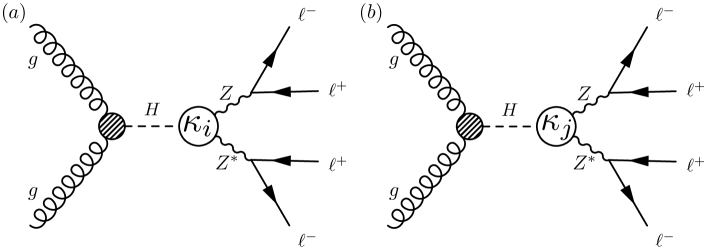
The “golden” Higgs to four-lepton channel (see Fig. 2) is quite sensitive, both for the discovery and for the subsequent measurement of the spin and parity properties of the Higgs boson Dell'Aquila:1985ve ; Nelson:1986ki ; Kniehl:1990yb ; Soni:1993jc ; Chang:1993jy ; Barger:1993wt ; Arens:1994wd ; Choi:2002jk ; Allanach:2002gn ; Buszello:2002uu ; Godbole:2007cn ; Kovalchuk:2008zz ; Keung:2008ve ; Antipin:2008hj ; Cao:2009ah ; Gao:2010qx ; DeRujula:2010ys ; Englert:2010ud ; Matsuzaki:2011ch ; DeSanctis:2011yc ; logan ; Gainer:2011xz ; oai:arXiv.org:1110.4405 ; Englert:2012ct ; Campbell:2012cz ; Campbell:2012ct ; Kauer:2012hd ; Kniehl:2012rz ; Moffat:2012pb ; Coleppa:2012eh ; Bolognesi:2012mm ; Boughezal:2012tz ; Stolarski:2012ps ; Cea:2012ud ; Kumar:2012ba ; Geng:2012hy ; Avery:2012um ; Masso:2012eq ; Chen:2012jy ; Modak:2013sb ; Kanemura:2013mc ; Gainer:2013rxa ; Isidori:2013cla ; Frank:2013gca ; Grinstein:2013vsa ; Caola:2013yja ; Banerjee:2013apa ; Sun:2013yra ; Anderson:2013afp ; Chen:2013waa ; Buchalla:2013mpa ; Chen:2013ejz ; Campbell:2013una ; Chen:2014pia ; Gonzalez-Alonso:2014rla ; Gainer:2014hha ; Chen:2014gka , and therefore plays an important role in the experimental study of the Higgs at the LHC Chatrchyan:2012jja ; Aad:2013xqa ; Chatrchyan:2013mxa ; 1523699 ; 1542341 ; 1542387 . Assuming that the putative Higgs is spin-zero, we can then characterize its couplings to $Z$ bosons, following Gainer:2014hha , using the Lagrangian

$$\mathcal{L}\supset\sum_{i=1}^{5}\kappa_{i}\mathcal{O}_{i}= -\kappa_{1}\frac{M_{Z}^{2}}{v}HZ_{\mu}Z^{\mu}-\frac{\kappa_{2}}{2v}HF_{\mu\nu}F^{\mu\nu}-\frac{\kappa_{3}}{2v}HF_{\mu\nu}\tilde{F}^{\mu\nu}$$ (25)

$$+\frac{\kappa_{4}M_{Z}^{2}}{M_{X}^{2}v}\Box HZ_{\mu}Z^{\mu}+\frac{2\kappa_{5}}{v}HZ_{\mu}\square Z^{\mu}.$$

Therefore, in general, the $HZZ$ couplings involve five parameters (up to lowest non-trivial dimension). Following the “Geolocating” approach Gainer:2013rxa , we can remove the degree of freedom associated with the partial width, leaving us with a “sphere” of four-dimensions. To explore this space fully, we may need to employ reweighting procedures, such as those described here.

Figure 3: Normalized distributions of the quantity $M_{Z_{2}}=\min{(M_{e^{+}e^{-}},M_{\mu^{+}\mu^{-}})}$ at parton-level. In each panel, the solid magenta distributions are obtained using events generated under various coupling hypotheses: a) $\kappa_{i}=(1,0,0,0,0)$, b) $\kappa_{i}=(0,1,0,0,0)$, and c) $\kappa_{i}=(0,0,1,0,0)$, while the solid blue distribution is obtained by directly generating events for a model with $\kappa_{i}=(0,0,0,0,1)$. Alternatively, we can obtain the same $\kappa_{5}\neq 0$ distribution, by recycling the events used for the solid magenta histograms, and reweighting them with the corresponding ratio of matrix elements squared. The results from such reweighting are shown by the dotted red distributions.

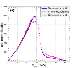
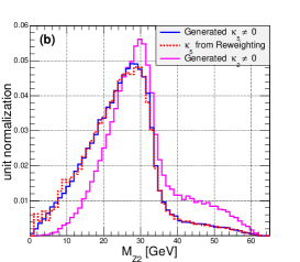
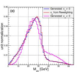
As an example of such analyses, in Fig. 3 we study the distribution of the smaller dilepton invariant mass $M_{Z_{2}}=\min{(M_{e^{+}e^{-}},M_{\mu^{+}\mu^{-}})}\,$ in the $2e2\mu$ final state. In each of the three panels in Fig. 3, the solid blue histogram is always the normalized $M_{Z_{2}}$ distribution for the pure $\kappa_{5}$ case, i.e. when $\kappa_{5}\neq 0$ and all other $\kappa_{i}$ ($i=1,\ldots,4$) are zero. On the other hand, the solid magenta histograms correspond to the case when only one of the other $\kappa_{i}$ couplings is turned on: $\kappa_{1}\neq 0$ in panel (a), $\kappa_{2}\neq 0$ in panel (b), and $\kappa_{3}\neq 0$ in panel (c). Our reweighting procedure now allows us to obtain the shape of the solid blue histogram by reweighting the corresponding magenta plot. The results are shown by the dotted red lines in Fig. 3. By comparing the solid blue and dotted red distributions, we observe a very good match, which validates our procedure.

However, it is not sufficient to show that the central bin values for each histogram are reproduced by the reweighting procedure. To perform statistical analyses using the reweighted histograms, we need to understand the error (or uncertainty) on the histogram bin values. Following Ref. Lyons:1986em , if there are $N$ events in a bin, each of which has weight $w_{k}$, then the value of that bin in the reweighted histogram is

$$T=\sum w_{k}\equiv N\langle w\rangle.$$ (26)

The error on $T$ is given by

$$\delta=\sqrt{\sum w_{k}^{2}}=\sqrt{N}\sqrt{\langle w^{2}\rangle}.$$ (27)

Clearly, in the special case of an unweighted histogram, $\delta$ yields $\sqrt{N}$ which reproduces the well-known expression from Poisson statistics. Combining Eqs. (26) and (27), and writing $\langle w^{2}\rangle$ in terms of the variance on the weights,

$$\sigma_{w}^{2}=\langle w^{2}\rangle-\langle w\rangle^{2},$$ (28)

we find the fractional error on the bin value in a weighted histogram to be given by

$$\frac{\delta}{T}=\frac{1}{\sqrt{N}}\sqrt{1+\frac{\sigma_{w}^{2}}{\langle w\rangle^{2}}}.$$ (29)

For the case of interest to us, the $w_{k}$ are the reweighting factors $R(A,\bm{\alpha},B,\bm{\beta})$ used to reweight events generated for model $A$, in order to obtain a histogram for model $B$. (Note that the value of $N$ is the same for the two models.) Since in general the reweighting factor varies from event to event, the variance (28) is nonzero. Thus, when we reweight, the statistical error increases, and Eq. (29) quantifies this effect.

Figure 4: The fractional error on each $M_{Z2}$ bin value, obtained by applying Eq. (29) to the red-dashed and magenta histograms from Fig. 3.

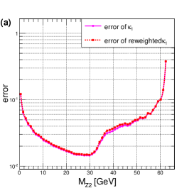
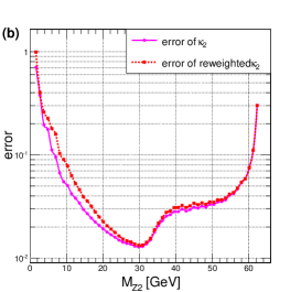
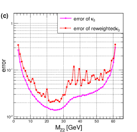
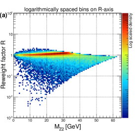
To provide a concrete demonstration of these effects, in Fig. 4(a-c) we show the fractional error, as calculated using Eq. (29), on each bin of the corresponding histograms from Fig. 3(a-c). In Fig. 4, solid magenta lines denote the fractional error (which scales as $1/\sqrt{N}$) in the original model with unweighted events, while the red dotted lines show the error on the corresponding histogram obtained from the same events using reweighting. In accordance with Eq. (29), the error is in general greater for the reweighted histogram, but not always — e.g., in Fig. 4(a), the errors before and after reweighting are essentially the same. To better illustrate the origin of the errors after reweighting, in Fig. 5 we provide two dimensional temperature plots of the reweighting factor, $R$, and the corresponding value of $M_{Z2}$ for each event. We see a clear correlation between the spread in the values of $R$ and the magnitude of the increase in the fractional errors in Fig. 4.

Figure 5: The values of the reweighting factor, $R(A,\bm{\alpha},B,\bm{\beta})$, and $M_{Z_{2}}$ for the events used to obtain the histograms in Fig. 3.

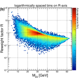
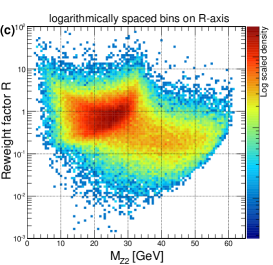
At this point, one might wonder how the errors on histograms which were reweighted from an initial model $A$ to another model $B$ compare to the errors on histograms built from unweighted events generated directly in model $B$. Since the error on the bin values in the unweighted histogram is $1/\sqrt{T}$, from Eqs. (26) and (29) we get

$$\bigg{(}\frac{\delta}{T}\bigg{)}/\bigg{(}\frac{1}{\sqrt{T}}\bigg{)}=\sqrt{\langle w\rangle}\sqrt{1+\frac{\sigma_{w}^{2}}{\langle w\rangle^{2}}},$$ (30)

where we assume sufficiently large statistics, so that the number of unweighted events is close to the expected value $T$. We see that the second factor in Eq. (30) always leads to an increase in the error when reweighting, in agreement with Fig. 4. On the other hand, the first factor, $\sqrt{\langle w\rangle}$, can be either larger or smaller than 1, depending on the relative weights between models $A$ and $B$. Using Eqs. (29) and (30), one can quantify the error from reweighting in the region of interest. If that error turns out to be unacceptably large for the task at hand, one can apply the procedures discussed below in Sec. 5 to further reduce those errors.

In Fig. 3 we presented distributions for the $M_{Z_{2}}$ variable, which we studied further in Figs. 4 and 5. However, we wish to emphasize that the variable whose distribution is obtained via reweighting could also be an optimized multivariate analysis-based variable such as the MELA KD Gao:2010qx ; Chatrchyan:2012jja , MEKD Avery:2012um , or the output of a boosted decision tree or neural network analysis. Hence reweighting can be used in tandem with sophisticated and powerful multivariate analysis methods Bhat:2010zz .

4.2 Changing Spin Assignments: The Antler Topology

Figure 6: Feynman diagrams for the antler topology in a) SUSY and b) MUED. We can study the MUED spin assignment in this topology by reweighting SUSY events, as demonstrated in the text.

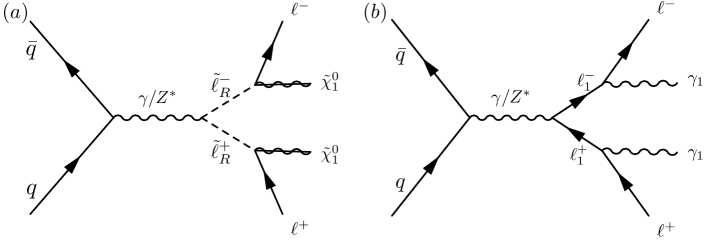
Extensive simplified model searches ArkaniHamed:2007fw ; Alwall:2008ag ; Alves:2011wf have been performed by the ATLAS and CMS collaborations in various channels ATLAS:2011lka ; Okawa:2011xg ; ATLAS:2011ffa ; Chatrchyan:2013sza . When performing a simplified model analysis, one generally fixes the spins of the particles involved in the simplified event topology. One common choice is to use SUSY spin assignments, though another possibility is to decay all particles by pure phase space. It is important to be able to interpret the results from these searches in the context of other models, with different spin assignments. A particularly well motivated example of an alternative spin assignment is provided by the minimal UED model (MUED) Cheng:2002iz .

To perform reinterpretations for different spin assignments, we need to recalculate cross sections, branching ratios, and efficiencies for the given study point in the new model. We can obtain cross sections and branching ratios for the new model point via theoretical formulae, but efficiencies generally must be obtained through MC simulation. We emphasize that we can recycle existing MC samples to determine these efficiencies for different new physics models in an efficient manner. In this subsection, we demonstrate the utilization of MC event samples generated for a SUSY model to perform a collider analysis of the MUED model, in the context of the “antler” topology Han:2009ss ; Edelhauser:2012xb depicted in Fig. 6. In particular we show distributions of collider observables, which could be used to discriminate between SUSY and MUED Battaglia:2005zf ; Datta:2005zs ; Meade:2006dw ; Athanasiou:2006ef ; Wang:2006hk ; Burns:2008cp . Numbering the leptons as $1$ for the $\ell^{-}$ and $2$ for the $\ell^{+}$, these variables are:

Figure 7: Distributions of various parton-level quantities which might be used to distinguish SUSY from MUED Edelhauser:2012xb . The SUSY parameter point used is the CMS LM6 study point LM6 ; in the UED scenario the Kaluza-Klein partners have the same mass as the corresponding superpartners.

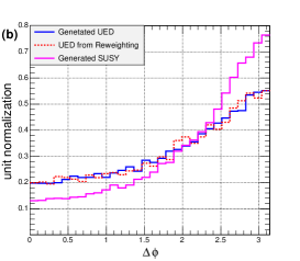
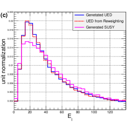
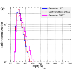
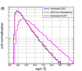
• $\cos(\theta_{B})$: A variable calculated from the pseudorapidity difference between the two leptons Barr:2005dz , defined by

  $$\cos(\theta_{B}) = \tanh\left(\frac{\Delta\eta_{12}}{2}\right),$$ (31)

  $$\Delta\eta_{12} = \eta_{1}-\eta_{2},\textrm{ with }\eta_{i}=\frac{1}{2}\ln\left(\frac{P_{i}+P_{iz}}{P_{i}-P_{iz}}\right).$$ (32)

• $\Delta\phi$: The azimuthal angular difference of the visible particles,

  $$\Delta\phi=\cos^{-1}\left(\frac{\vec{P}_{1T}\cdot\vec{P}_{2T}}{|\vec{P}_{1T}|\,|\vec{P}_{2T}|}\right).$$ (33)

• $E_{\ell}$: The energy of a lepton $E_{\ell}.$

• $M_{\ell^{-}\ell^{+}}$: The invariant mass of the two leptons.

• $\sqrt{\hat{s}}_{\min}$: An estimator of the mass scale of the hard scattering, proposed in Konar:2008ei ; Konar:2010ma , calculated for the antler event topology assuming a particular value for the $\tilde{\chi}_{1}^{0}$ mass. Since in practice we would scan over this “trial” mass, for definiteness we use the correct or “truth” value of this quantity in the analyses presented here. The definition of $\sqrt{\hat{s}}_{\min}$ is

  $$\sqrt{\hat{s}}_{\min}=\sqrt{M_{\ell^{-}\ell^{+}}^{2}+|\vec{P}_{1T}+\vec{P}_{2T}|^{2}}+\sqrt{4m_{\tilde{\chi}_{1}^{0}}^{2}+\not\!\!E_{T}^{2}}\,.$$ (34)

• $\sqrt{\hat{s}}$: The actual partonic center-of-mass energy.

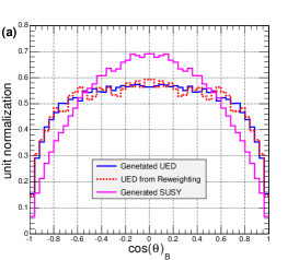
Distributions of the above observables are shown in Fig. 7. For the various quantities, we show

1. (solid magenta lines) The distribution of the quantity obtained from MC simulation of the CMS LM6 LM6 SUSY parameter point, where the mass of the right-handed scalar lepton, $m_{\tilde{\ell}_{R}}$ is $176.62$ GeV and the neutralino mass $m_{\tilde{\chi}_{1}^{0}}$ is $158.18$ GeV.

2. (solid blue lines) The distribution of the quantity obtained from MC simulation of a MUED parameter point where the mass of the Kaluza-Klein (KK) lepton is $176.62$ GeV, and the mass of the KK photon is $158.18$ GeV, matching the masses of the SUSY particles in the LM6 scenario.

3. (dotted red lines) The distribution of the quantity that one would obtain for the MUED parameter point, evaluated by the reweighting of events generated for the SUSY parameter point.

The MC samples used to generate these distributions consist of $100,000$ parton level events at the $14$ TeV LHC. Fig. 7 suggests that MUED analyses can in fact be performed by reweighting SUSY MC events, allowing the efficient probing of non-standard spin assignments at the LHC. One could extend this technique beyond MUED to all other possible spin assignments for a given event topology with given masses. In particular, one could set robust and model independent limits on new physics in the following way. Among all possible spin assignments (or more generally, parameter values), identify the case which is most difficult to test experimentally, and use it to present limits from experimental searches. The conservative bounds set in this way will be valid for all other spin assignments as well.

4.3 Jet Clustering, Event Selection, and Detector Response

Figure 8: A conceptual diagram illustrating the use of reweighting for events which are passed through detector simulation. As noted above, if a physics model, $I$, shares the same phase space with a model $J$, we can perform Monte Carlo analyses of model $J$ by reweighting detector level events of model $I$ using a reweighting value calculated using “truth” MC events at parton or generator level, $\frac{|M_{J}(Gen)|^{2}}{|M_{I}(Gen)|^{2}}.$ We denote actual event generations by solid lines and mark calculations for the reweighting procedure with dashed lines. The weight of an event in the given model is indicated by the shade of gray. The effects of showering, hadronization, detector simulation, and jet clustering are shown conceptually by the reshaping of the events which are rectangular at generator level and oddly shaped after detector simulation. Clearly the detector level events are the same whether or not we are reweighting (hence have the same shapes in our figure). Also, detector level events either pass cuts or fail cuts regardless of whether reweighting is employed.

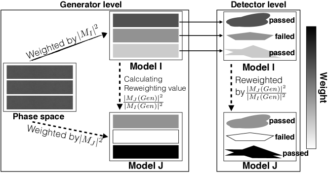
Parton level information can be distorted by various factors, including showering, hadronization, jet clustering, and detector response. All of these can “deform” the phase space of generated particles. But, as noted in Section 2, the relative weights in various models for a given observed event depend only on the parton level amplitudes for the event in each model. We present a conceptual picture of this reweighting procedure in Fig. 8.

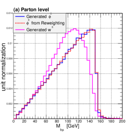
To illustrate this point numerically, we simulate $t\bar{t}$ production at $14$ TeV LHC, where the top-quark (anti-top quark) decays into a $W^{+}$ ($W^{-}$) boson or charged Higgs $\phi^{+}$ ($\phi^{-}$), see Fig. 9. Our goal is to evaluate the performance of the reweighting procedure described in Fig. 8, including effects that we did not account for in the parton-level examples described in Sections 4.1 and 4.2. Specifically, we generated $100,000$ parton level events with MadGraph5(aMC) v.2.1.0, passed the events to PYTHIA 6.4, and performed detector simulation with Delphes v.3.0.12. For jet clustering, we used the anti-$k_{t}$ algorithm with $\Delta R=0.5$. For the reconstruction of visible particles, we employ default smearing factors and lepton tagging efficiencies. We apply basic analysis cuts with $p_{T}(e)>10$ GeV, $p_{T}(\mu)>5$ GeV and $p_{T}(j)>30$ GeV and do not require $b$-tagging in our analysis.

Figure 9: To demonstrate the use of reweighting events involving detector simulation and jet clustering, we study top quark pair production, followed by decays involving a $b$-jet and either (a) the $W^{\pm}$ boson, as in the SM, or (b) a charged Higgs, $\phi^{\pm}$. As we show, the charged Higgs scenario (b) can be analyzed using SM dilepton $t\bar{t}$ events (a) through reweighting. Due to the mass dependence of Higgs couplings, the lepton from charged Higgs decay is always a muon and never an electron.

When the top quark decays into a bottom quark and a charged Higgs boson, the invariant mass distribution of the bottom quark and the corresponding lepton from the charged Higgs boson decay will have a triangular shape (the solid blue line in Fig. 10(a)). On the other hand, the invariant mass distribution of the $b$-quark and the corresponding lepton from a $W^{\pm}$ decay will have a non-trivial shape (solid magenta lines in Fig. 10(a)). These two cases can be easily related by reweighting at the parton level, as shown by the red dotted histogram in Fig. 10(a).

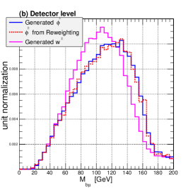
At the detector level, the $b$-quark is reconstructed as a jet, thus we select the two highest $p_{T}$ jets to be our $b$ jets. In order to study the effects of combinatorics separately, in Fig. 10(b) we show an intermediate (and unphysical) case where we use MC truth information to select the correct jet to be paired with the muon. We see that the reweighting procedure correctly reproduces the distributions of kinematic variables computed in terms of reconstructed objects.

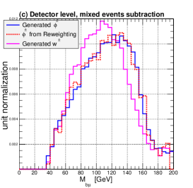
Finally, in Fig. 10(c) we show the same three distributions, only this time ignoring the MC truth information and fully accounting for the combinatorics. In order to reduce the contamination from combinatorial pairing errors, we use the mixed event subtraction method Hinchliffe:1996iu , where we add both possible pairings in a given event, then subtract a pairing of the muon with a jet from a different event. We emphasize that the point of these analyses is that a distribution made through reweighting is identical to the actual distribution made with a MC events generated for the hypothesis in question.

Figure 10: Invariant mass distributions, $m_{b\mu}$, of $b$-jets and the muon for events generated using the topologies shown in Fig. 9. The variable $m_{b\mu}$ contains information about the spin of the intermediate particle, $W^{\pm}$ or $\phi^{\pm}$. In (a) we plot this quantity at parton level, pairing the muon with the $b$ from the same top decay. In $(b)$, we use events which have undergone realistic simulation, i.e. they are showered, hadronized, and passed through fast detector simulation and jet clustering. To separate the effects of detector simulation, etc. from the effects of combinatorics, we use truth information to select the correct jet to pair with the lepton. In $(c)$, which was also generated using realistic simulation, we include the effects of combinatorics by not using truth information (to model the actual experimental situation) and instead using the mixed event subtraction method Hinchliffe:1996iu to suppress contributions from incorrect parings of jets and muons.

5 Possible extensions

As noted in Section 4 above, reweighting events generated using model $I$ to obtain distributions in model $J$ may become problematic for two main reasons. Firstly, in a phase space region where the cross section for the new model $J$ is high, while the cross-section for the reference model $I$ is low, the region is sampled by relatively few MC events. Secondly, the spread in the reweighting factors for events in the given bin may become large. Both of these effects are described by Eq. 29. We are obviously interested in minimizing the errors on histograms, but at the same time, we want to keep as low as possible the number of events which need to be processed by full MC simulation.

We therefore suggest three practical procedures that can be used to mitigate issues related both to undersampling and to the spread on reweighting factors, and possibly to help understand systematic effects.

1. Targeted Generation: In this procedure, whenever the error in a reweighted histogram obtained for model $J$ becomes greater than a certain threshold, one generates additional new events in the undersampled region that are phase space “neighbors” of the events already in the bin. The simplest way to think of this is to divide phase space $\mathcal{P}$ into two non-overlapping regions, $\mathcal{N}$ and $\overline{\mathcal{N}}$, where $\mathcal{N}$ describes a phase space region where additional event generation is desired, and $\overline{\mathcal{N}}$ is the rest of the phase space. Then we generate events for model $J$ only in region $\mathcal{N}$. Distributions for $J$ will then be obtained by reweighting the events generated for model $I$ in the $\overline{\mathcal{N}}$ and for events generated for model $J$ in the region $\mathcal{N}$. If one then wishes to obtain distributions for a third model, $K$, one will reweight events generated for model $I$ in region $\overline{\mathcal{N}}$ and the events generated for model $J$ in region $\mathcal{N}$, in each case using a reweighting factor involving the appropriate models.

2. Regions of Overlap: A related approach is to generate large samples of unweighted events at several benchmarks in parameter space, which we label $I_{1}$, $I_{2}$, etc. One then obtains distributions $D_{1}$, $D_{2}$, etc. for model $J$ by reweighting events generated for model $I_{1}$, $I_{2}$, etc. If the benchmarks are chosen appropriately, every important region in phase space for model $J$ can be described with low errors by reweighted events generated for some model $I_{j}$, hence avoiding the undersampling issues described above. Also, the comparison of the values of the distribution obtained from different choices of unweighted events may allow for the calculation of systematic errors from this procedure.

3. Optimized Sample: A third, and quite distinct approach to optimizing reweighting procedures for large parameter space is to optimize the choice of model $I$ to avoid undersampling in as much of the parameter space as possible. In general, this would be performed by maximizing an integral over the parameter space (possibly weighted by some prior or importance measure) of a function representing the errors that will be obtained on bins of the desired histograms. This appears to be a hard integral to perform in practice, so reasonable approaches will probably involve approximation to some degree. It is also unclear whether even an optimized model would be as efficient as generating events for at least the several benchmarks in parameter space described in the previous item.

6 Conclusions

We have presented and described in detail a procedure aimed at surmounting the experimental challenges presented by the multiplicity of theoretical models, which may each, in turn, have large parameter spaces. We realize that the procedure presented here is not totally unknown to experimentalists (particularly in the special case of parton distribution function reweighting Tricoli:2008ev ). However, given the importance of this challenge, we felt it important to highlight the potential of this method, especially for the study of large BSM parameter spaces.

Specifically, we have shown how reweighting events using “truth” information from generator-level Monte Carlo events, including the momenta of invisible particles, makes possible the detailed study of large signal parameter spaces and/or large numbers of signal models at the level of detail needed for experimental purposes. We demonstrated this in several motivated physics examples and also illustrated potential issues which can arise, including an explicit discussion of the errors on the weighted histograms generated from reweighting.

There are several advantages of our method:

• Given a large existing sample for some theory model $I$, we gain speed in generating an effective fullsim sample for another theory model $J$ by avoiding detector simulation, hadronization, showering and fragmentation.

• All existing fullsim samples can be resurrected for the study of new models.

• The reweighting is computationally very quick and simple - for example, there is no need to integrate over the momenta of any invisible particles.

• Reweighting also allows the interactions between theorists and experimentalists to be maximally efficient - the experimentalists are handling the fullsim MC generation, while the theorists are providing only the parton-level functions for reweighting the events.

We conclude with the simple recommendation that in order to be able to implement the procedure described here, when generating fullsim samples, one should make sure to record and store the generator-level information which is needed for reweighting.