Galaxy Cluster Scaling Relations Measured with APEX-SZ

Abstract

We present thermal Sunyaev-Zel’dovich effect (SZE) measurements for 42 galaxy clusters observed at 150 GHz with the APEX-SZ experiment. For each cluster, we model the pressure profile and calculate the integrated Comptonization $Y$ to estimate the total thermal energy of the intracluster medium (ICM). We compare the measured $Y$ values to X-ray observables of the ICM from the literature (cluster gas mass $M_{\rm{gas}}$, temperature $T_{X}$, and $Y_{X}=M_{\rm{gas}}T_{X}$) that relate to total cluster mass. We measure power law scaling relations, including an intrinsic scatter, between the SZE and X-ray observables for three subsamples within the set of 42 clusters that have uniform X-ray analysis in the literature. We observe that differences between these X-ray analyses introduce significant variability into the measured scaling relations, particularly affecting the normalization. For all three subsamples, we find results consistent with a self-similar model of cluster evolution dominated by gravitational effects. Comparing to predictions from numerical simulations, these scaling relations prefer models that include cooling and feedback in the ICM. Lastly, we measure an intrinsic scatter of $\sim 28$ per cent in the $Y-Y_{X}\,$ scaling relation for all three subsamples.

1 Introduction

As the largest gravitationally collapsed objects in the Universe, clusters of galaxies provide a unique opportunity to study the evolution of large-scale structure. The distribution and abundance of clusters is sensitive to both the geometry of the universe and the growth of density perturbations (e.g., Haiman et al., 2001; Weller et al., 2002). Currently, cluster-based constraints on cosmology are limited by systematic uncertainties in relating observables to cluster masses. Most of the cluster mass is in the form of dark matter and therefore is not directly observable. Instead, cluster masses are inferred through scaling relations with observable signals such as X-ray luminosity, galaxy velocity distribution, weak-lensing shear and Sunyaev-Zel’dovich effect (SZE) brightness.

Under the model of self-similarity, where cluster evolution is dominated by gravitational processes, cluster mass scales with observable signals through simple power law relations (Kaiser, 1986). In this model, the intracluster medium (ICM) is in hydrostatic equilibrium, for which the scaling to cluster mass can be predicted for a given observable. However, self-similarity does not take into account the role of non-thermal mechanisms such as turbulent gas motions in estimating cluster mass. This simple model also neglects the effects of physical processes internal to the cluster such as feedback from active galactic nuclei and star formation. Numerical simulations predict that while the power law exponent of SZE scaling relations will be consistent with self-similarity, the normalization does depend on the internal cluster astrophysics (Motl et al., 2005; Nagai, 2006; Lau et al., 2009). An empirical measurement of the scaling relations therefore informs models of cluster astrophysics, progressing towards the needed calibration for cosmology.

Currently, cluster surveys are operating in the optical (e.g., Gilbank et al., 2011), X-ray (e.g., Vikhlinin et al., 2009; Mantz et al., 2010), and the millimeter (e.g., Carlstrom et al., 2011; Swetz et al., 2011; Planck Collaboration, 2014a) wavelength regimes. However, optical and X-ray measurements of clusters suffer from cosmological dimming, and only the brightest and most massive clusters are detected at high redshifts ($z>1$). In contrast, the millimeter-wavelength thermal SZE (Sunyaev & Zel’dovich, 1972), where Cosmic Microwave Background (CMB) photons inverse-Compton scatter off hot intracluster electrons, is redshift-independent. SZE surveys with sufficient resolution to resolve clusters, such as those performed with the South Pole Telescope (Reichardt et al., 2013) and the Atacama Cosmology Telescope (Hasselfield et al., 2013) detect clusters with a mass selection nearly independent of redshift.

Precision cosmology requires that mass-observable scaling relations be characterized with a high level of accuracy, including both the measurement uncertainty and the intrinsic scatter from cluster-to-cluster differences. Numerical simulations suggest that SZE observations are relatively insensitive to the details of cluster astrophysics (e.g., Hallman et al., 2006; Nagai, 2006), resulting in low intrinsic scatter scaling relations and a tighter constraint on cluster mass. Previous measurements of SZE scaling relations include interferometric observations from the OVRO/BIMA (Bonamente et al., 2008) and SZA (Culverhouse et al., 2010; Marrone et al., 2012) arrays as well as imaging studies with the South Pole Telescope (Andersson et al., 2011; Plagge et al., 2010; Benson et al., 2013), BOLOCAM (Sayers et al., 2011), Atacama Cosmology Telescope (Marriage et al., 2010), and the Planck mission (Planck Collaboration XI, 2011). In general, those studies find that observational SZE scaling relations agree with expectations based on self-similarity and that simulations including additional non-adiabatic physics are preferred.

While cluster samples selected from large surveys (both SZE and X-ray) have well-known selection functions, studies such as the one presented in this paper that target known clusters often select them in an ad hoc manner. The influence of this sample selection on SZE scaling relations is unknown.

In this paper, we study how the SZE signal scales with X-ray observables related to cluster mass using observations from the APEX-SZ imaging bolometer array. We measure SZE scaling relations using X-ray observables ($Y_{X}$, $M_{\rm{gas}}$, and $T_{X}$) as proxies for the total cluster mass. APEX-SZ observed a small set of 11 clusters selected from the REFLEX X-ray survey (referred to as the REFLEX-DXL sample (Zhang et al., 2006)) as well as an additional 31 clusters selected in an ad hoc manner. Within this full sample are clusters drawn from the Zhang et al. (2008, hereafter Z08) and Mantz et al. (2010, hereafter M10) samples. We measure power law scaling relations for each of these three subsamples (REFLEX-DXL, Z08, M10) and compare the results to the expectations of the self-similar model as well as numerical simulations that incorporate different physical processes in the ICM. We compare the results between the three cluster samples as well as to the full APEX-SZ sample to investigate the effects of sample selection and uniform analysis on the measured power law and intrinsic scatter of the SZE scaling relations. In this paper, we assume the WMAP7+BAO+$H_{0}$ $\Lambda$CDM best-fit cosmology in which $H_{0}=70.4$ km $\rm{s}^{-1}$ $\rm{Mpc}^{-1}$, $\Omega_{M}=0.272$, and $\Omega_{\Lambda}=0.728$ (Komatsu et al., 2001).

The structure of the paper is as follows. Section 2 reviews the SZE and the associated scaling relations. Section 3 introduces the clusters in this study and observations thereof. Section 4 briefly describes the data reduction process for the APEX-SZ instrument. We present the SZE-X-ray scaling relations and discuss these results in Section 5. A summary and an outlook on future work are provided in Section 7.

2 The Thermal Sunyaev-Zel’dovich Effect

The SZE occurs when photons from the CMB inverse Compton scatter off hot electrons in the intracluster medium to higher energies (Sunyaev & Zel’dovich, 1972). This process distorts the CMB blackbody spectrum with an amplitude proportional to the gas pressure integrated along the line-of-sight. In units of temperature the change is

$$\frac{\Delta T_{\rm{SZE}}}{T_{\rm{CMB}}}=\int f(x,T_{e})\cdot n_{e}\sigma_{T}\frac{k_{B}T_{e}}{m_{e}c^{2}}dl\equiv f(x,T_{e})\cdot y,$$ (1)

where $n_{e}$ and $T_{e}$ are the electron density and temperature of the ICM, $T_{\rm{CMB}}$ is the temperature of the CMB, $\sigma_{T}$ is the Thomson cross-section, $k_{B}$ is the Boltzmann constant, and $m_{e}c^{2}$ is the electron rest mass energy. The integrated pressure is often parametrized in terms of the Comptonization, $y$. The frequency dependence $f(x,T_{e})$ is given by

$$f(x,T_{e})=\left(x\frac{e^{x}+1}{e^{x}-1}-4\right)(1+\delta_{\rm{SZE}}(x,T_{e})),$$ (2)

where $x=h\nu/k_{B}T_{\rm{CMB}}$ and $\delta_{\rm{SZE}}(x,T_{e})$ is a correction for relativistic electrons (see, e.g., Nozawa et al., 2000). For frequencies below 217 GHz, the SZE manifests itself as a decrement in the CMB spectrum, while at frequencies above 217 GHz the SZE results in an increment. Equation 1 demonstrates two important characteristics of the SZE. First, the SZE is redshift independent since its surface brightness is expressed as a fractional change in the CMB temperature. Second, the dependence on integrated pressure directly measures the thermal energy of the ICM.

The Comptonization integrated over the solid angle of the cluster on the sky,

$$Y=\int yd\Omega,$$ (3)

measures the total thermal energy of a cluster, and is therefore expected to be a robust proxy for total mass. In this work, we integrate a parametric model of $Y$ to a radius of $r_{500}$, the radius at which the mean matter density of the cluster is 500 times the critical density of the Universe, $\rho_{c}(z)=3H_{0}^{2}E(z)^{2}/8\pi G$. Assuming that clusters are in hydrostatic equilibrium, the integrated Comptonization scales as a function of the ICM properties according to

$$Yd_{A}^{2} \propto f_{\rm{gas}}T_{e}^{5/2}E(z)^{-1}$$

$$Yd_{A}^{2} \propto f_{\rm{gas}}^{-2/3}M_{\rm{gas}}^{5/3}E(z)^{2/3},$$ (4)

where $E(z)$ is the expansion rate of the universe normalized to its present value, $E(z)=H(z)/H_{0}=\sqrt{\Omega_{M}(1+z)^{3}+\Omega_{\Lambda}}$, $f_{\rm{gas}}$ is the gas mass fraction, and $d_{A}$ is the angular diameter distance of the cluster (Bonamente et al., 2008). A third proxy for cluster mass can be constructed from the combination of temperature and gas mass, $Y_{X}=M_{\rm{gas}}T_{X}$ (Kravtsov et al., 2006). $Y$ scales with $Y_{X}$ as

$$Yd_{A}^{2}\propto Y_{X},$$ (5)

and is expected to have lower intrinsic scatter than $Y-T$ or $Y-M_{\rm{gas}}$ due to the anti-correlation of systematic deviations between $T$ and $M_{\rm{gas}}$.

3 Observations

APEX-SZ (Schwan et al., 2011) was a transition-edge-sensor (TES) bolometer array located on the 12-meter Atacama Pathfinder Experiment (APEX) telescope in northern Chile (Güsten et al., 2006). The focal plane comprised a total of 280 bolometers distributed on six wafers which were cooled with closed-cycle refrigerators to an average operating temperature of $\sim$300 mK and read out using frequency domain multiplexing (Dobbs et al., 2012). The APEX-SZ experiment imaged SZE decrements at 150 GHz with arcmin resolution over a 23 arcmin field of view (FOV). Additional details of the APEX-SZ instrument are presented in Dobbs et al. (2006) and Schwan et al. (2011).

APEX-SZ completed two commissioning and seven observing runs from 2005 to 2010. During this time, APEX-SZ observed the 42 clusters presented here for a total of approximately 760 hours. APEX-SZ executed a circular drift scan pattern that concentrated the integration time in a region around the known cluster coordinates while limiting overhead time due to telescope turn-arounds. The telescope repeated the circular scan while centered on a constant azimuth and elevation, allowing the target to drift through the FOV. After completing between 11 and 20 circles (4–7 seconds per circle), the telescope slewed to track the target and then repeated the circular pattern. The radius of each circle ($6$–$12$ arcmin) was chosen from the expected radial extent of each cluster to ensure that the detectors observed the sky background during each scan. These scans resulted in a sky coverage area of approximately $0.75\mbox{${}^{\circ}$}\times 1.0\mbox{${}^{\circ}$}$.

Clusters were targeted based on the availability of published X-ray measurements. In general, massive clusters ($T_{X}>6$ keV) were selected and the sample included both dynamically relaxed and disturbed clusters. Additionally, APEX-SZ targeted clusters from the REFLEX-DXL X-ray sample (Zhang et al., 2006), which is discussed in further detail in 5.3. Coordinates and map depth for each cluster are given in Table 1.

Table 1: Summary of cluster properties.

Cluster Name	Right Ascension	Declination	redshift	Map Deptha
	(h m s)	(∘ ′ ′′)		($\mu K$ CMB)
Abell 2744	00 14 18.6	-30 23 15.4	0.307	12
Abell 2813	00 43 24.5	-20 37 31.2	0.292	21
Abell 209	01 31 52.6	-13 36 35.5	0.209	16
XLSS J022145.2-034617	02 21 45.2	-03 46 17.4	0.430	7
RXCJ0232.2-4420	02 32 18.8	-44 20 51.9	0.284	17
Abell 383	02 48 03.3	-03 31 43.6	0.187	14
RXCJ0437.1+0043	04 37 09.5	+00 43 54.5	0.284	14
MS0451.6-0305	04 54 11.3	-03 00 52.6	0.550	21
Abell 520	04 54 09.0	+02 55 18.0	0.203	14
RXCJ0516.6-5430	05 16 35.2	-54 30 36.8	0.294	10
RXCJ0528.9-3927	05 28 52.5	-39 28 16.7	0.284	11
RXCJ0532.9-3701	05 32 55.9	-37 01 34.5	0.275	16
Abell 3404	06 45 30.0	-54 13 42.1	0.164	13
1ES 0657-56	06 58 30.2	-55 56 33.7	0.296	19
Abell 907	09 58 21.9	-11 03 48.2	0.160	11
XMMXCSJ095940.8+023111.3	09 59 40.8	+02 31 11.3	0.720	14
RXCJ1023.6+0411	10 23 39.6	+04 11 12.0	0.291	12
MS1054.4-0321	10 56 59.0	-03 37 37.0	0.830	13
MACSJ1115.8+0129	11 15 51.9	+01 29 55.0	0.355	16
Abell 1300	11 31 54.7	-19 55 40.5	0.308	18
RXCJ1206.2-0848	12 06 12.3	-08 48 06.0	0.439	18
XMMUJ1230.3+1339	12 30 16.9	+13 39 04.3	0.975	11
RDCSJ1252-2927	12 52 54.4	-29 27 17.0	1.240	8
MACSJ1311.0-0311	13 11 01.7	-03 10 37.6	0.494	12
Abell 1689	13 11 29.3	-01 20 26.7	0.184	19
RXCJ1347.5-1144	13 47 30.8	-11 45 09.0	0.451	28
MACSJ1359.1-1929	13 59 10.3	-19 29 24.0	0.447	27
Abell 1835	14 01 01.9	+02 52 35.5	0.253	36
RXCJ1504.1-0248	15 04 07.6	-02 48 16.0	0.215	21
Abell 2163	16 15 46.0	-06 08 54.0	0.203	30
Abell 2204	16 32 47.1	+05 34 32.3	0.152	10
MACSJ1931.8-2635	19 31 49.6	-26 34 34.0	0.352	30
RXCJ2011.3-5725	20 11 27.1	-57 25 09.8	0.279	11
RXCJ2014.8-2430	20 14 49.7	-24 30 30.0	0.161	15
MACSJ2046.0-3430	20 46 00.5	-34 30 17.0	0.423	15
RXCJ2214.9-1359	22 14 57.4	-14 00 10.8	0.503	23
XMMXCSJ2215.9-1738	22 15 58.0	-17 38 02.5	1.450	11
XMMUJ2235.3-2557	22 35 20.6	-25 57 42.0	1.393	9
RXCJ2243.3-0935	22 43 21.4	-09 35 43.0	0.447	20
Abell S1077	22 58 48.1	-34 47 59.4	0.313	17
Abell 2537	23 08 22.0	-02 11 30.0	0.297	11
RXCJ2337.6+0016	23 37 37.8	+00 16 15.5	0.278	20

^aMap depth is measured within the central arcminute from the standard deviation of 500 jackknife noise map realizations.

Table 2: Summary of cluster X-ray properties.

Cluster Name	$T_{X}$	Ref.	$M_{\rm{gas}}$	Ref.	$Y_{X}$
	keV		$10^{13}\rm{M}_{\odot}$		$10^{13}$keV $\rm{M}_{\odot}$
Abell 2744	$10.1\pm 0.3$	2	$10\pm 2$	2	$101\pm 20$
	$8.53\pm 0.37$	3	$20.1\pm 2.1$	3	$171.5\pm 19.4$
Abell 2813	$7.7\pm 0.3$	2	$6\pm 1$	2	$46\pm 8$
	$7.0\pm 0.4$	1	$5.8\pm 0.6$	1	$40.6\pm 4.8$
	$7.59\pm 0.77$	3	$9.2\pm 1.4$	3	$69.8\pm 12.8$
Abell 209	$7.1\pm 0.3$	1	$7.8\pm 0.8$	1	$55.4\pm 6.1$
	$8.23\pm 0.66$	3	$14.4\pm 1.8$	3	$118.5\pm 17.6$
XLSS J022145.2-034617	$4.8_{-0.5}^{+0.6}$	7	$\cdots$	$\cdots$	$\cdots$
RXCJ0232.2-4420	$7.0\pm 0.3$	2	$9\pm 2$	2	$63\pm 14$
	$6.6\pm 0.3$	1	$8.9\pm 0.9$	1	$58.7\pm 6.5$
	$10.06\pm 2.31$	3	$14.5\pm 2.5$	3	$145.9\pm 42.9$
Abell 383	$4.7\pm 0.2$	1	$3.3\pm 0.4$	1	$15.5\pm 2.0$
RXCJ0437.1+0043	$5.1\pm 0.3$	2	$5\pm 1$	2	$26\pm 5$
MS0451.6-0305	$6.6_{-0.6}^{+0.7}$	11	$12.1_{-0.2}^{+0.2}$	11	$79.7_{-7.4}^{+8.5}$
Abell 520	$7.23\pm 0.23$	3	$13.7\pm 1.5$	3	$99.1\pm 11.3$
RXCJ0516.6-5430	$7.5\pm 0.3$	2	$8\pm 2$	2	$60\pm 15$
	$6.7\pm 0.5$	1	$7.8\pm 0.9$	1	$52.3\pm 7.2$
RXCJ0528.9-3927	$7.2\pm 0.4$	2	$9\pm 1$	2	$65\pm 8$
	$6.6\pm 0.5$	1	$8.7\pm 0.7$	1	$57.4\pm 6.4$
	$7.8\pm 0.85$	3	$15.2\pm 1.7$	3	$118.6\pm 18.5$
RXCJ0532.9-3701	$9.5\pm 0.4$	2	$6\pm 1$	2	$57\pm 10$
	$7.7\pm 0.6$	1	$5.7\pm 0.7$	1	$43.9\pm 6.4$
Abell 3404	$7.6\pm 0.3$	1	$9.0\pm 1.1$	1	$68.4\pm 8.8$
1ES 0657-56	$10.6\pm 0.2$	2	$18\pm 3$	2	$191\pm 32$
	$10.7\pm 0.4$	1	$17.6\pm 0.2$	1	$188.3\pm 19.5$
	$11.70\pm 0.22$	3	$26.1\pm 2.4$	3	$305.4\pm 28.7$
Abell 907	$5.8\pm 0.3$	1	$4.3\pm 0.5$	1	$24.9\pm 3.2$
XMMXCSJ095940.8+023111.3	$7.3_{-0.8}^{+1.4}$	9	$\cdots$	$\cdots$	$\cdots$
RXCJ1023.6+0411	$8.38\pm 0.44$	3	$10.8\pm 1.0$	3	$90.5\pm 9.6$
MS1054.4-0321	$8.3\pm 0.7$	14	$\cdots$	$\cdots$	$\cdots$
MACSJ1115.8+0129	$9.20\pm 0.98$	3	$9.9\pm 1.1$	3	$91.1\pm 14.0$
Abell 1300	$9.2\pm 0.4$	2	$8\pm 2$	2	$74\pm 19$
	$9.35\pm 1.67$	3	$21.6\pm 2.8$	3	$202.0\pm 44.6$
RXCJ1206.2-0848	$10.71\pm 1.29$	3	$21.9\pm 2.9$	3	$234.5\pm 42.0$
XMMUJ1230.3+1339	$6.0_{-1.2}^{+1.6}$	4	$3\pm 1$	4	$18_{-6}^{+7}$
RDCSJ1252-2927	$6.6_{-1.2}^{+1.5}$	6	$0.66_{-0.10}^{+0.09}$	6	$4.4_{-1.0}^{+1.2}$
MACSJ1311.0-0311	$6.2\pm 0.7$	11	$4.6_{-0.1}^{+0.1}$	11	$28.5_{-3.3}^{+3.3}$
Abell 1689	$8.5\pm 0.2$	1	$10.5\pm 1.4$	1	$89.2\pm 12.1$
RXCJ1347.5-1144	$10.75\pm 0.83$	3	$24.8\pm 2.7$	3	$266.6\pm 35.6$
MACSJ1359.1-1929	$6.73\pm 0.96$	13	$\cdots$	$\cdots$	$\cdots$
Abell 1835	$8.4\pm 0.3$	1	$11.8\pm 1.4$	1	$99.1\pm 12.3$
	$9.00\pm 0.25$	3	$14.1\pm 0.6$	3	$126.9\pm 6.4$
RXCJ1504.1-0248	$8.00\pm 0.44$	3	$12.5\pm 1.3$	3	$100.0\pm 11.8$
Abell 2163	$12.27\pm 0.90$	3	$44.0\pm 4.5$	3	$539.9\pm 67.9$
Abell 2204	$7.6\pm 0.2$	1	$8.4\pm 1.0$	1	$63.8\pm 7.8$
MACSJ1931.8-2635	$7.47\pm 1.40$	3	$11.4\pm 1.5$	3	$85.2\pm 19.5$
RXCJ2011.3-5725	$3.23\pm 0.34$	3	$3.7\pm 0.7$	3	$12.0\pm 2.6$
RXCJ2014.8-2430	$5.63\pm 0.11$	12	$7.1_{-0.1}^{+0.1}$	12	$39.9_{-1.1}^{+1.1}$
MACSJ2046.0-3430	$5.81\pm 1.02$	13	$\cdots$	$\cdots$	$\cdots$
RXCJ2214.9-1359	$8.8\pm 0.7$	8	$\cdots$	$\cdots$	$\cdots$
XMMXCSJ2215.9-1738	$7.4_{-1.4}^{+2.1}$	6	$0.38\pm 0.09$	6	$2.8_{-0.9}^{+1.0}$
XMMUJ2235.3-2557	$6.0_{-1.8}^{+2.5}$	5	$0.95_{-0.12}^{+0.11}$	6	$5.7_{-1.9}^{+2.5}$

Table 3: continued

Summary of cluster X-ray properties. Cluster Name $T_{X}$ Ref. $M_{\rm{gas}}$ Ref. $Y_{X}$ keV $10^{13}\rm{M}_{\odot}$ $10^{13}$keV $\rm{M}_{\odot}$ RXCJ2243.3-0935 $8.24\pm 0.92$ 3 $19.8\pm 2.4$ 3 $163.2\pm 26.9$ Abell S1077 $8.0\pm 0.5$ 10  $\cdots$  $\cdots$  $\cdots$ Abell 2537 $7.9\pm 0.7$ 2 $7\pm 1$ 2 $55\pm 9$ $7.6\pm 0.7$ 1 $6.5\pm 0.7$ 1 $49.4\pm 7.0$ $7.63\pm 0.86$ 3 $8.2\pm 1.1$ 3 $62.6\pm 11.0$ RXCJ2337.6+0016 $9.6\pm 0.3$ 2 $8\pm 1$ 2 $77\pm 10$ $7.5\pm 0.5$ 1 $8.1\pm 0.7$ 1 $60.8\pm 6.6$

1. Zhang et al. (2008) $kT_{(0.2-0.5)r_{500}}$

2. Zhang et al. (2006) $kT_{(0.1-0.5)r_{500}}$

3. Mantz et al. (2010) $kT_{(0.15-0.5)r_{500}}$

4. Fassbender et al. (2011) $kT_{r<71\mbox{${}^{\prime\prime}$}}$

5. Mullis et al. (2005) $kT_{r<50\mbox{${}^{\prime\prime}$}}$

6. Culverhouse et al. (2010) $kT_{r<30\mbox{${}^{\prime\prime}$}}$

7. Pacaud et al. (2007) $kT_{r<80\mbox{${}^{\prime\prime}$}}$

8. Ebeling et al. (2007) $kT_{70kpc<r<r_{1000}}$

9. Mehrtens et al. (2012)

10. De Filippis et al. (2004) $kT_{r<2.5\mbox{${}^{\prime}$}}$

11. Maughan et al. (2008) $kT_{(0.15-1)r_{500}}$

12. Pratt et al. (2009) $kT_{(0.15-1)r_{500}}$

13. Allen et al. (2008) $kT_{r<r_{2500}}$

14. Branchesi et al. (2007) $kT_{r<84\mbox{${}^{\prime\prime}$}}$

4 APEX-SZ Data Analysis

Raw APEX-SZ timestream data contain the faint SZE cluster signal, scan synchronous signals due to ground pick-up and instrumental thermal fluctuations, atmospheric fluctuations, and instrument noise. In order to measure the SZE surface brightness accurately, the array properties must be well characterized and contamination cleaned from the data.

4.1 Beams and Calibration

The beam position and shape for each bolometer in the focal plane are measured from a daily raster scan of a calibration target (Mars, Uranus, or Saturn). In addition to the 58 arcsec FWHM Gaussian main beam, APEX-SZ beams exhibit significant sidelobes (Schwan et al., 2011). We characterize the sidelobes by mapping the individual detector beams and combining them into a composite beam. The total beam area, including the Gaussian main beam and the sidelobes, is then taken into account during further calibration. The beam size is also corrected to account for the angular extent of the source and detector saturation effects.

Absolute flux calibration is performed based on the overall amplitude of response for each detector from a raster scan on a known celestial source. APEX-SZ observed two primary flux calibrators: Mars and Uranus. The planetary disk size and brightness temperature are taken from the Rudy model for Mars (Rudy et al., 1987; Muhleman & Berge, 1991) and from the JCMT FLUXES model for Uranus. As described in Halverson et al. (2009), we refine the absolute brightness temperatures for Mars and Uranus using WMAP results (Hinshaw et al., 2009; Weiland et al., 2011) to improve calibration accuracy. We find that the Rudy temperatures are systematically higher than WMAP by a factor of $1.052\pm 0.01$. The calculation of this factor includes the extrapolation of the Rudy and WMAP 94 GHz brightness temperatures to 150 GHz, 1.016$\pm$ 0.009, which is included in the total calibration uncertainty. Similarly, we use the data of Griffin & Orton (1993) to extrapolate the WMAP7 94 GHz measurement of Uranus to $T_{150\rm{GHz}}=100.4\pm 5.3$ K.

Several times during observations primary planetary calibrators were unavailable due to angular proximity to the Sun. The stable Galactic H II regions RCW38 and IRAS12073-6233 were used as secondary calibrators during these periods, with brightness temperatures bootstrapped from back-to-back scans of the primary and secondary calibrators.

The measured calibration is corrected for differences in atmospheric opacity between the data and calibration scans using the measured value of precipitable water vapour (PWV) from the APEX radiometer. Following Sayers et al. (2011), we extrapolate the atmospheric optical depth based on the ATM model (Pardo et al., 2001) and correct accordingly.

In addition to the calibration scan, routine pointing scans of bright quasars are performed throughout the night. We find an average pointing jitter of approximately 5.7 arcsec in both azimuth and elevation. This is significantly less than the size of the APEX-SZ beam and has a negligible effect on the measurements presented here.

Combining the corrections discussed in this section (beam solid angle, calibrator temperature, atmospheric opacity) with the uncertainty in the frequency band center (see Halverson et al., 2009) we estimate the Gaussian uncertainty in the flux calibration to be $\pm$8 per cent.

4.1.1 Gain Fluctuations

Ideally, the responsivity of each bolometer is constant despite changing amounts of incident optical power (Lee et al., 1996). However, when a bolometer is biased near the upper edge of the superconducting transition, the responsivity changes as a result of varying optical power from three sources: the elevation dependence of atmospheric airmass, the overall atmospheric opacity, and the power from an astronomical source. The last effect is sub-dominant, but it cannot be neglected for the case of a bright calibrator. For most detectors in the APEX-SZ array, suppression of responsivity is approximately a linear function of incident optical power. However, some channels exhibit more extreme changes.

We measure the responsivity of each bolometer using the elevation($\epsilon$) dependent signal $d_{i}\propto A_{\csc,i}\csc(\epsilon)$ introduced by the circular scan pattern. This is repeated for every two minutes of data, normalizing by the changing zenith emissivity to measure $A_{\csc,i}$. Channels that exhibit strong nonlinear response are discarded from use in further analysis. For the remaining channels, we model the response as a linear function and use it to correct the absolute flux calibration, discarding data that deviate more than $2.5\sigma$ from the best-fit model. Data with extremely large overall correction factors (greater than 50 per cent) are discarded.

We also correct for two second order effects. First, as a bright calibration source is scanned, variable responsivity will slightly distort the measured beam shape. Second, the fractional solid angle of the sidelobes relative to the main beam will be affected.

Based on the rms scatter around the best-fit gain models, we estimate the uncertainty in the responsivity corrections to be $\pm$5 per cent. Combining this uncertainty with the calibration uncertainty from the previous section, we find that the total uncertainty in the APEX-SZ temperature calibration is $\pm$10 per cent.

4.2 Timestream Processing

The APEX-SZ data set was measured in widely varying atmospheric conditions, a significant challenge when trying to measure the relatively faint SZE signal. In general, the atmospheric signal is highly correlated between bolometers as spatial fluctuations in the atmosphere are much larger than the APEX-SZ FOV. Additionally, the bolometers exhibit a correlated signal due to heating of the detector array from telescope vibrations. We employ several different filtering techniques to clean the data, similar to Halverson et al. (2009). In order to optimize the final maps, filtering is tailored to the specific needs of each target with the goal of sufficiently removing contamination and minimizing noise while preserving cluster signal.

4.2.1 Initial Data Conditioning

The first step to condition APEX-SZ timestreams is to parse the data into separate circles made on the sky according to the scan pattern. The circles are grouped together based on a common central azimuth and elevation and data not in a circle set are discarded.

Initial channel and data cuts are performed on the indexed data based on several criteria. Channels that are optically unresponsive (optical efficiency less than 6 per cent) are rejected. APEX-SZ timestreams occasionally exhibit large spikes or glitches in one or many bolometers due to either cosmic rays or electrical interference. Glitches are located and removed from the timestreams using both the timestream derivative and a simple S/N threshold cut. When a glitch is simultaneously detected in several channels (more than 7 per cent), that particular section of data is discarded for all channels. As a final step, channels with excess noise between 12 and 18 Hz are discarded.

After the initial data cuts we deconvolve an optical time constant for each channel from the timestreams. The median measured optical time constant for APEX-SZ bolometers is $\sim$12 ms, however, it is as high as $\sim$60 ms for some channels. To prevent the amplification of high frequency noise during deconvolution, an additional low-pass filter ($F=\exp\left[-(f/f_{0})^{6}\right]$) is applied. We define $f_{0}=2*v_{\rm{scan}}/\rm{FWHM}$ where $v_{\rm{scan}}$ is the median scan velocity of the telescope and $\rm{FWHM}$ is the full width at half-maximum of the APEX-SZ beam.

4.2.2 Removal of Timestream Contamination

The final step in processing the timestream data is to remove the dominant atmospheric and thermal signals. The majority of the timestream cleaning is performed through a combination of two methods: high-pass time-domain filters and the subtraction of spatial polynomial functions across the array, taking advantage of the correlation between bolometers.

An initial high-pass filter removes the static offset for each channel as well as low-frequency noise in the timestreams. Removing the timestream signal due to stage heating is especially important because the subsequent spatial template removal steps use relative gain coefficients that are based solely on the atmospheric response. The high-pass filtering is implemented in two forms: an N-order polynomial removal and a Butterworth frequency domain filter. The polynomial filter, described in detail in Halverson et al. (2009), simultaneously removes a scan synchronous cosecant signal.

Figure 1: The power spectral density (PSD) of an APEX-SZ timestream at three different stages of timestream reduction. The black line represents the raw data in units of readout counts. The blue line shows the power remaining after initial data cuts are performed, optical time constants are deconvolved, and a high-pass filter is applied. The decrease in low-frequency power is due to the high-pass step, whereas roll-off at high-frequencies is a result of the low-pass filter included in the time constant deconvolution. The red line shows the power spectrum after spatial template removal and polynomial removal steps are performed, removing the remaining low-frequency contamination and completing the cleaning of the data.

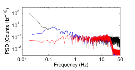
After the first high-pass filter, we remove a 2-dimensional spatial polynomial function across the array (Sayers, 2007; Halverson et al., 2009) at each sample in the timestream. During this process, referred to as spatial template removal, we fit the polynomial either across the entire array, or individually for each of the six detector wafers to improve removal of correlated signals on scales smaller than the $0.4^{\circ}$ field-of-view. Often, this filter is applied multiple times, discarding channels with excess variance in between. A final polynomial removal is performed to remove any remaining contamination. Figure 1 shows the power spectrum of an APEX-SZ timestream at three different steps in the reduction process.

4.3 Map Making & Transfer Function

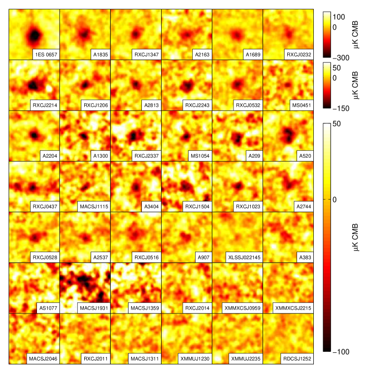
Once the timestreams are filtered, we create sky maps by binning the timestream data into $10\times 10$ arcsec pixels. Sky coordinates for each bolometer are determined from the absolute telescope boresight pointing and individual bolometer positional offsets. As in Halverson et al. (2009), bolometers and scans are combined with a minimum variance weighting for each cluster. The resulting set of 42 sky maps is shown in Figure 2. Each map has been convolved with a one arcmin FWHM Gaussian for visual presentation. However, all subsequent analysis is performed on the unsmoothed version.

In conjunction with the sky map, we quantify the effects of the APEX-SZ instrumental beam and analysis filtering on the sky signal. A simulated cluster map, created using the profile discussed in Section 4.4.1, is convolved with the composite beam profile of the array and mapped into timestreams using the telescope pointing information. Each data cut and filtering process performed on the real cluster data is repeated on these timestreams. The filtered simulation is mapped and coadded using the same minimum variance weights as the cluster map. An individualized transfer function map, $\mathbf{K}$, is created for each cluster by normalizing the Fourier transform of the filtered map to that of the original simulation.

Figure 2: Sky maps for each of the APEX-SZ cluster positions in signal-to-noise units. The data for each 15 x 15 square arcmin map have been filtered to remove contaminating signals. Therefore, the maps show an attenuated representation of the sky. Each map has been additionally convolved with a one arcmin Gaussian.

We create difference noise maps for each cluster to characterize the map noise. In this process, random halves of the individual scan maps are multiplied by -1 before coadding. This removes any astrophysical signal that is consistent between all maps, including primary CMB anisotropy. To account for the noise due to the CMB, we convolve a realization of the CMB created from the Planck + WP best-fit power spectrum (Planck Collaboration, 2014b) with a CMB transfer function (created in the same way as the cluster transfer function) and add it to the difference noise map. In addition to the CMB, a contribution from a background of point sources is expected. We find that the power from Poisson distributed point sources (Hall et al., 2010; Shirokoff et al., 2010), including an extra 50 per cent variance due to lensing (Hezaveh et al., 2013), is negligible in comparison to the instrument noise.

4.4 Cluster Signal Modeling

4.4.1 Parametric Models

In order to calculate the integrated cluster signal, we need to extrapolate the measured cluster signal to spatial scales that have been filtered out due to timestream processing and the angular resolution of the instrument. We adopt the universal pressure profile of Arnaud et al. (2010),

$$P_{e}(r)=\frac{P_{0}}{(r/r_{s})^{\gamma}[1+(r/r_{s})^{\alpha}]^{(\beta-\gamma)/\alpha}}.$$ (6)

Here $P_{0}$ is the normalization of the pressure profile, $r_{s}$ is the scale radius, and ($\alpha,\beta,\gamma$) describe the slope of the profile for $r\approx r_{s}$, $r>r_{s}$ and $r<r_{s}$, respectively. The scale radius is often defined in terms of a concentration parameter $c_{500}$, $r_{s}=r_{500}/c_{500}$. Proposed by Nagai et al. (2007), this generalized Navarro-Frenk-White model (GNFW), is a generalization of the numerical results from Navarro et al. (1997) for the distribution of mass in a dark matter halo. Arnaud et al. (2010) combined simulations and X-ray observations to measure a best-fit model of ($c_{500}$, $\alpha,\beta,\gamma$) = (1.177, 1.0510, 5.4905, 0.3081), which we use for the measurements presented here. Applying the ideal gas law, $P_{e}=n_{e}kT_{e}$, to Equation 6 and substituting into Equation 1 the SZE profile becomes

$$\frac{\Delta T_{\rm{SZE}}}{T_{\rm{CMB}}} = \int f(x,T_{e})\cdot\frac{\sigma_{T}}{m_{e}c^{2}}P_{e}(r)dl.$$ (7)

We reparametrize Equation 7 in terms of a normalization $\Delta T_{0}$,

$$\Delta T_{\rm{SZE}}=\Delta T_{0}\int\frac{1}{(r/r_{s})^{\gamma}[1+(r/r_{s})^{\alpha}]^{(\beta-\gamma)/\alpha}}dl.$$ (8)

Due to the compact scan pattern and strong atmospheric filtering required, the APEX-SZ data poorly constrain power on scales larger than 10 arcmin in the maps. Therefore, we infer $r_{500}$ from the X-ray based $r_{500}-T$ scaling relation of Vikhlinin et al. (2006) for each cluster and fix the model centroid at the X-ray centroid. The Arnaud et al. (2010) profile for each cluster serves as the simulated input for creating the individualized transfer functions described in $\S$4.3 and is used to fit for the normalization, $\Delta T_{0}$.

4.4.2 Likelihood Analysis

We calculate the likelihood for each model as a function of $\Delta T_{0}$, $\mathcal{L}\propto e^{-\chi^{2}(\Delta T_{0})/2}$. First, we create a 2-dimensional model map $\mathbf{M}(\Delta T_{0})$ and convolve it with the transfer function map $\mathbf{K}$, $\mathbf{M}^{\prime}(\Delta T_{0})=\mathbf{K}*\mathbf{M}(\Delta T_{0})$. The model $\mathbf{M}^{\prime}(\Delta T_{0})$ and sky maps $\mathbf{D}$ are binned into 1-arcmin radial bins around the X-ray centroid. Using the central 10 arcmin of these profiles, we construct the $\chi^{2}$ statistic,

$$\chi^{2}=(\mathbf{D}-\mathbf{M}^{\prime}(\Delta T_{0}))^{\rm{T}}\mathbf{C}_{n}^{-1}(\mathbf{D}-\mathbf{M}^{\prime}(\Delta T_{0})),$$ (9)

where $\mathbf{C}_{n}$ is the noise covariance matrix estimated by averaging 500 radially-binned difference noise realizations. The best-fit parameters along with the X-ray based $\theta_{500}=r_{500}/d_{A}$ and respective probability to exceed (PTE) are given in Table 4.

For each cluster, we calculate the spherical integral of the assumed model profile within the X-ray defined $r_{500}$ and use the measured $\Delta T_{0}$ to estimate the integrated Comptonization $Y_{500}$. We use the work of Nozawa et al. (2000) and the X-ray temperatures from Table 2 to calculate the relativistic correction $\delta_{\rm{SZE}}$ to the frequency dependent term in Equation 2. On average, this correction is of order $\sim 5$ per cent. The measured values of $Y_{500}$ are given in Table 4.

5 Results

5.1 Cluster Observables

We use the method described in Section 4.4 to measure the spherically-integrated Comptonization for each cluster. We assume the cluster follows an Arnaud et al. (2010) pressure profile (see Equation 6) with radius $r_{500}$, where $r_{500}$ is inferred from the Vikhlinin et al. (2006) $r-T_{X}$ relation.

We use three different proxies for total cluster mass: spectroscopic X-ray temperature, gas mass, and $Y_{X}$, the values for which are taken from the literature. The redshifts and X-ray parameters for the 42 clusters included in this sample are given in Table 2 along with the references. For clusters found in more than one of the REFLEX-DXL, Z08, or M10 subsamples, the additional parameter values are also given. All measurements were made with either the XMM-Newton or Chandra X-ray observatories. X-ray temperatures are used that were derived from temperature maps with the central region excluded when available. Inclusion of the core region can lead to an underestimated global temperature for the cool-core clusters present within our sample. $M_{\rm{gas}}$ values, and by extension $Y_{X}$, were available for only 35 clusters.

Table 4: APEX-SZ Model Fits

Cluster Name	$\Delta T_{0}$	$\theta_{500}$	Ref.	PTE	$Y_{500}$
	($\mu$K CMB)	(′′)			($10^{-10}sr$)
Abell 2744	$-439\pm 80$	$311.3$	2	0.11	$1.51\pm 0.28$
	$-433\pm 80$	$284.8$	3	0.07	$1.23\pm 0.23$
Abell 2813	$-482\pm 74$	$281.7$	2	0.14	$1.33\pm 0.20$
	$-498\pm 78$	$267.9$	1	0.24	$1.24\pm 0.19$
	$-503\pm 80$	$279.6$	3	0.14	$1.37\pm 0.22$
Abell 209	$-472\pm 76$	$360.9$	1	0.24	$2.14\pm 0.34$
	$-440\pm 78$	$390.1$	3	0.32	$2.34\pm 0.42$
XLSS J022145.2-034617	$-200\pm 48$	$158.6$	8	0.21	$0.17\pm 0.04$
RXCJ0232.2-4420	$-611\pm 73$	$274.3$	2	$7.8\times 10^{-3}$	$1.60\pm 0.19$
	$-622\pm 67$	$266.0$	1	$4.1\times 10^{-3}$	$1.52\pm 0.16$
	$-581\pm 68$	$332.1$	3	$7.8\times 10^{-3}$	$2.27\pm 0.26$
Abell 383	$-264\pm 71$	$320.5$	1	0.79	$0.93\pm 0.25$
RXCJ0437.1+0043	$-341\pm 72$	$232.2$	2	$3.8\times 10^{-5}$	$0.63\pm 0.13$
MS0451.6-0305	$-638\pm 159$	$153.2$	12	0.21	$0.52\pm 0.13$
Abell 520	$-354\pm 50$	$373.9$	4	$1.2\times 10^{-5}$	$1.72\pm 0.24$
RXCJ0516.6-5430	$-221\pm 54$	$276.2$	2	$1.3\times 10^{-8}$	$0.59\pm 0.14$
	$-221\pm 59$	$260.3$	1	$3.6\times 10^{-9}$	$0.52\pm 0.14$
RXCJ0528.9-3927	$-418\pm 64$	$278.5$	2	$1.2\times 10^{-4}$	$1.13\pm 0.17$
	$-426\pm 61$	$266.0$	1	$5.5\times 10^{-5}$	$1.04\pm 0.15$
	$-444\pm 61$	$290.4$	3	$1.9\times 10^{-5}$	$1.31\pm 0.18$
RXCJ0532.9-3701	$-572\pm 79$	$331.3$	2	$5.6\times 10^{-3}$	$2.21\pm 0.31$
	$-553\pm 76$	$296.6$	1	$4.5\times 10^{-3}$	$1.70\pm 0.23$
Abell 3404	$-462\pm 64$	$464.4$	1	$8.4\times 10^{-3}$	$3.47\pm 0.48$
1ES 0657-56	$-1113\pm 49$	$329.5$	2	$3.3\times 10^{-6}$	$4.27\pm 0.19$
	$-1123\pm 47$	$331.1$	1	$3.6\times 10^{-6}$	$4.35\pm 0.18$
	$-1106\pm 49$	$347.1$	3	$8.5\times 10^{-6}$	$4.74\pm 0.21$
Abell 907	$-334\pm 52$	$411.8$	1	0.71	$1.95\pm 0.30$
XMMXCSJ095940.8+023111.3	$-112\pm 93$	$139.2$	10	$1.4\times 10^{-3}$	$0.076\pm 0.063$
RXCJ1023.6+0411	$-440\pm 62$	$295.7$	4	0.16	$1.35\pm 0.19$
MS1054.4-0321	$-808\pm 106$	$123.8$	15	0.98	$0.43\pm 0.06$
MACSJ1115.8+0129	$-290\pm 88$	$262.1$	4	0.12	$0.70\pm 0.21$
Abell 1300	$-497\pm 97$	$295.6$	2	0.73	$1.53\pm 0.30$
	$-458\pm 96$	$298.1$	3	0.83	$1.43\pm 0.30$
RXCJ1206.2-0848	$-756\pm 103$	$237.8$	4	0.18	$1.51\pm 0.21$
XMMUJ1230.3+1339	$-204\pm 97$	$91.6$	5	0.31	$0.059\pm 0.028$
RDCSJ1252-2927∗	$-22\pm 90$	$79.2$	7	0.28	$(4.89\times 10^{-3})\pm 0.020$
MACSJ1311.0-0311∗	$-72\pm 85$	$161.8$	12	0.88	$0.066\pm 0.077$
Abell 1689	$-1043\pm 93$	$444.3$	1	0.23	$7.21\pm 0.64$
RXCJ1347.5-1144	$-1002\pm 126$	$233.1$	4	0.24	$1.93\pm 0.24$
MACSJ1359.1-1929∗	$-109\pm 112$	$183.5$	14	0.02	$0.13\pm 0.13$
Abell 1835	$-810\pm 105$	$333.7$	1	0.42	$3.16\pm 0.41$
	$-770\pm 118$	$346.0$	3	0.36	$3.24\pm 0.50$
RXCJ1504.1-0248	$-584\pm 112$	$374.4$	4	0.52	$2.86\pm 0.55$
Abell 2163	$-684\pm 105$	$494.0$	4	0.90	$5.96\pm 0.92$
Abell 2204	$-623\pm 52$	$497.4$	4	0.01	$5.37\pm 0.45$
MACSJ1931.8-2635∗	$-37\pm 117$	$236.6$	4	0.20	$0.072\pm 0.228$
RXCJ2011.3-5725	$-109\pm 78$	$185.6$	3	0.16	$0.13\pm 0.09$
RXCJ2014.8-2430∗	$-26\pm 89$	$403.1$	13	0.58	$0.14\pm 0.50$
MACSJ2046.0-3430	$-132\pm 108$	$177.7$	14	0.72	$0.14\pm 0.12$
RXCJ2214.9-1359	$-730\pm 91$	$191.8$	9	$4.4\times 10^{-4}$	$0.94\pm 0.12$
XMMXCSJ2215.9-1738∗	$-14\pm 145$	$74.1$	7	0.24	$(2.68\times 10^{-3})\pm 0.028$
XMMUJ2235.3-2557∗	$33\pm 153$	$68.6$	6	0.51	$(-5.35\times 10^{-3})\pm 0.025$
RXCJ2243.3-0935	$-846\pm 111$	$204.1$	4	0.15	$1.23\pm 0.16$
Abell S1077	$-234\pm 112$	$270.9$	11	0.08	$0.60\pm 0.29$
Abell 2537	$-408\pm 70$	$281.7$	2	0.02	$1.13\pm 0.19$
	$-424\pm 71$	$276.0$	1	0.03	$1.13\pm 0.19$
	$-398\pm 75$	$276.6$	3	0.02	$1.06\pm 0.20$
RXCJ2337.6+0016	$-398\pm 73$	$330.1$	2	0.12	$1.53\pm 0.28$
	$-386\pm 79$	$289.9$	1	0.18	$1.13\pm 0.23$

$Y_{500}$ is the spherical integration of best-fit pressure profile within $r_{500}$. Non-detections are denoted with ^∗. References correspond to those in Table 2 and denote the X-ray measurement of $kT$ used to determine $r_{500}$. Values are given for each subsample where appropriate: [1] Z08, [2] REFLEX-DXL, [3] M10.

5.2 Regression Analysis

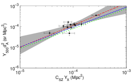
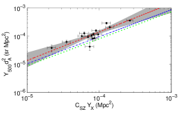
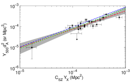
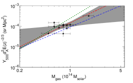
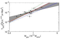
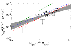
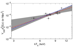
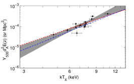
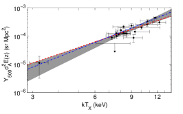
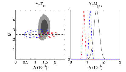
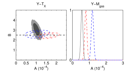
To derive best-fit scaling relations parameters we perform a regression analysis of the data shown in Figure 3. We assume that the data follow the power law relationship,

$$Y_{500}d_{A}^{2}E(z)^{\delta}=A\cdot\left(\frac{X}{X_{0}}\right)^{B},$$ (10)

where $A$ is the normalization, $B$ is the power law exponent, and $X$ denotes an X-ray observable. A pivot point, $X_{0}$, is chosen for each observable ($T_{0}$ = 7.5 keV, $M_{\rm{gas},0}=1.0\times 10^{14}M_{\odot}$, $Y_{X,0}=8.0\times 10^{14}M_{\odot}\rm{keV}$) to reduce the correlations between $A$ and $B$. We use the self-similar values of $\delta=(1,-2/3,0)$, respectively (see Equation 2). The intrinsic astrophysical scatter in the scaling relation is represented through a log-normal distribution with mean $\mu=\rm{log}_{10}A+B\cdot\rm{log}_{10}(X/X_{0})$ and variance $\sigma_{\rm{log_{10}(Y)}}^{2}$ in the base 10 logarithm of the distribution.

This regression is often performed in the log basis, where Equation 10 transforms to a simple linear relationship with Gaussian intrinsic scatter. In agreement with Kelly (2007, hereafter K07), we find from simulated data sets that common methods for linear regression with uncertainty in both the x- and y-variables, such as those in Press et al. (2007) and Weiner et al. (2006), introduce systematic bias into the measured parameters. The regression parameters are further biased by the symmetrization and transformation of the $Y_{500}$ likelihood distribution from the linear basis to the logarithmic basis. Lastly, the measured $Y_{500}$ non-detections in the APEX-SZ data cannot be fully represented in the log basis. For example, when we place a prior that $Y_{500}>0$ and perform a linear regression using the Bayesian method of sampling the posterior probability from K07, we find that the resulting maximum likelihood parameters are biased at the $1-2\sigma$ level.

To address the difficulties introduced by the log basis, we instead perform the regression analysis in the linear basis. We construct the likelihood of the scaling relations parameters from the probability densities of $Y_{500}$ measured with APEX-SZ and the X-ray observable (e.g., $Y_{X}$). We approximate the measured probabilities in $Y_{500}$ as asymmetric Gaussian distributions. Following the methodology of K07, we model the distribution of $X$ as a weighted sum of Gaussian functions. We sample the posterior likelihood distribution using an MCMC method with a Metropolis-Hastings algorithm. Using simulated data sets with X-ray properties based on those of the APEX-SZ cluster sample, we find that we are able to recover unbiased estimates of the scaling relation parameters.

Figure 3: $Y_{500}$ - $Y_{X}$, $Y_{500}$ - $M_{\rm{gas}}$, and $Y_{500}$ - $T_{X}$ scaling relations for the REFLEX-DXL (left column) and Z08 (middle column) and M10 (right column) cluster samples. The black points show the APEX-SZ measured values given in Table 4. Non-detections are plotted as 95 per cent upper limits. The shaded region depicts the 68 per cent confidence interval of the power law for the three-parameter fit. Also shown is the maximum likelihood result for the case where the exponent is fixed to the self-similar value (red dashed). For comparison, we plot the best-fit results from Planck Collaboration XI (2011) (blue dot-dash), Plagge et al. (2010) (dark green dot), and Andersson et al. (2011) (light green dot).

5.3 $Y_{500}-Y_{X},Y_{500}-M_{\rm{gas}},Y_{500}-T_{X}$ Relations

We fit the three scaling relations described in the previous section for three different subsamples within the APEX-SZ cluster sample. These subsamples are created based on the different X-ray analyses available: the REFLEX-DXL clusters, clusters from the analysis of Z08, and clusters from the analysis of M10. By restricting our scaling relations to subsamples with uniform X-ray analysis, we avoid the systematic bias and inflated uncertainty that results from different analysis choices (see Section 6.1.2). Several clusters are common between these three samples. For these cases, the X-ray parameters from the desired sample are used when modelling each cluster and fitting the scaling relation.

APEX-SZ observed 11 of the 13 clusters from the X-ray selected REFLEX-DXL cluster sample (Zhang et al., 2006). The remaining two clusters were not observed due to restrictions in accessible sky area. These clusters have an X-ray luminosity $L_{X}>5.9\times 10^{44}$ ergs $\rm{s}^{-1}$ in the ROSAT-ESO Flux Limited X-ray (REFLEX) galaxy cluster survey (Böhringer et al., 2004) and fall within a narrow redshift range, $0.27<z<0.31$. Zhang et al. (2006) observed the REFLEX-DXL clusters with the XMM-Newton satellite and measured the X-ray temperature and gas mass for each.

The second sample for which we fit the scaling relations includes 15 of the 37 clusters from the Local Cluster Substructure Survey (LoCuSS) measured by Z08. These X-ray luminous clusters occupy a wider redshift range $0.14\leq z\leq 0.3$ than the REFLEX-DXL sample. Using observations from the XMM-Newton satellite, these authors modelled the X-ray emission for each cluster to measure the X-ray temperature and gas mass.

Finally, the APEX-SZ sample includes 19 of the 94 clusters observed by M10. In contrast to the two other subsamples, the M10 X-ray properties were measured using both the Chandra and ROSAT telescopes, with a cross-calibration between the two data sets. Additionally, these clusters occupy a slightly larger range in redshift, $0.20\leq z\leq 0.45$.

Beyond the follow-up of the REFLEX-DXL subsample, many of the APEX-SZ clusters were selected in an ad hoc manner. We are unable to quantify the influence of this selection on the Z08 and M10 samples, resulting in an unknown level of systematic bias and uncertainty.

The maximum likelihood regression parameters and 68 per cent confidence intervals for all three samples are given in Table 5 and shown in Figure 3. We also give results for the cases where we fix the power law exponent to the self-similar values.

5.3.1 The REFLEX-DXL, Z08, & M10 Samples

First, we consider our constraints on the power law exponent $B$ for all three scaling relations, shown in Table 5. We find for the REFLEX-DXL sample that $B$ is consistent with self-similar expectations for all three scaling relations. In contrast, for the Z08 sample $Y_{500}-T_{X}\,$relation, we find a marginally steeper power law than expected in the self-similar case and measured for the REFLEX-DXL sample. We measure the exponent for the $Y_{500}-M_{\rm{gas}}\,$relation to be consistent between the three samples, however, these values are marginally lower than the self-similar expectation.

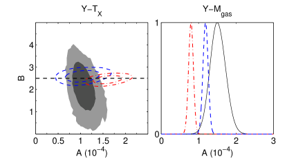
Next, we examine our measurements of the power law normalization $A$. For both the $Y_{500}-Y_{X}\,$and $Y_{500}-M_{\rm{gas}}\,$relations the M10 sample has a significantly lower $A$ (more than $3.3\sigma$ and $2.3\sigma$, respectively) than the other two samples. The normalization of the $Y_{500}-T_{X}\,$relation is consistent for the REFLEX-DXL and M10 samples, while the Z08 sample suggests a higher value. We compare our measurements for the $Y_{500}-M_{\rm{gas}}$ and $Y_{500}-T_{X}$ to the numerical simulations of Nagai (2006) (see Figure 4). These simulations agree well with the self-similar model. We therefore find similar tension between the measured $Y_{500}-M_{\rm{gas}}\,$exponent for all three samples and the simulations as for the comparison to self-similarity.

Different models of cluster gas physics are expected to mostly influence the scaling relation normalization (Motl et al., 2005; Nagai, 2006; Lau et al., 2009). For this reason, we consider the result where $B$ has been fixed to the self-similar value. As shown in Figure 4, the $Y_{500}-T_{X}\,$results for all three samples and the $Y_{500}-M_{\rm{gas}}\,$results for the REFLEX-DXL and Z08 samples favour simulations that include cooling and feedback over those with only standard gas dynamics. In contrast, the lower normalization for the M10 sample $Y_{500}-M_{\rm{gas}}\,$relation causes a preference for standard gas dynamics. For all three samples, the $Y_{500}-M_{\rm{gas}}\,$conclusions are weak because of the measured tension in the exponent.

The third free parameter in our regression model, $\sigma_{\rm{log_{10}(Y)}}$, quantifies the amount of scatter in the scaling relation not due to measurement uncertainties in $\rm{log_{10}}(Y_{500})$. We transform the values of $\sigma_{\rm{log_{10}(Y)}}$ from Table 5 into the fractional scatter, $\sigma_{Y}/Y=\sigma_{\rm{log_{10}(Y)}}/\rm{log}_{10}(e)$, commonly used in the literature. We measure $\sim$28 per cent ($\sigma_{\rm{log_{10}(Y)}}\approx 0.12$) intrinsic scatter for all three samples. Kravtsov et al. (2006) demonstrated that $Y_{X}$ is a more robust mass proxy than $T_{X}$ or $M_{gas}$. Because $Y$ and $Y_{X}$ measure similar quantities (Equation 5), we expect that $Y_{500}-Y_{X}\,$will have the lowest intrinsic scatter of the three scaling relations. As anticipated the $Y_{500}-M_{\rm{gas}}\,$relation exhibits an increased level of intrinsic scatter (35 per cent). The $Y_{500}-T_{X}\,$relation, however, has different values of intrinsic scatter depnding on the sample (ranging from 14 per cent to 37 per cent). We discuss these differences further in Section 6.

5.3.2 Comparison with Previous Experiments

There are four main observational studies with which we directly compare our $Y_{500}$ scaling relations. Planck Collaboration XI (2011, hereafter P11) and Planck Collaboration (2014a, hereafter P13) present SZE scaling relations using the Planck satellite (the early and 2013 results, respectively) in combination with X-ray data using the XMM-Newton satellite. Plagge et al. (2010, S10) and Andersson et al. (2011, S11) constrain SZE scaling relations using the South Pole telescope. Results from these studies are compared to the APEX-SZ results in Figure 3.

The APEX-SZ results for all three samples agree well with both the P11 and P13 constraints on the $Y_{500}-M_{\rm{gas}}\,$and $Y_{500}-Y_{X}\,$exponents. S11 explore $Y_{500}-Y_{X}\,$and likewise measure an exponent consistent with the APEX-SZ result. S10 evaluate both $Y_{500}-M_{\rm{gas}}\,$and $Y_{500}-Y_{X}\,$and measure exponents which are higher than the APEX-SZ values (approximately $1.6\sigma$ for the most consistent sample, REFLEX-DXL). However, these authors note that their results vary significantly when using different values of gas mass from the literature.

To compare the measured APEX-SZ power law normalization of the $Y_{500}-Y_{X}\,$relation for the REFLEX-DXL sample (given in Table 5) to previous measurements we transform our normalization parameter to $A^{\prime}=A\times 10^{-4}/8\times 10^{14}/C_{SZ}$, where $C_{SZ}=\sigma_{th}/m_{e}c^{2}\mu_{e}m_{p}$ (Arnaud et al., 2010). In the case where $B=1$, the ratio of $A^{\prime}=Y_{500}d_{A}^{2}/Y_{x}$ is a function of the differences between the mass-weighted and spectroscopic cluster temperatures.

We find for all three subsamples that the $Y_{500}-Y_{X}\,$normalizations are in some tension with previous observations. The REFLEX-DXL ($A^{\prime}=1.18_{-0.11}^{+0.21}$) and Z08 ($A^{\prime}=1.41\pm 0.15$) samples suggest higher normalizations than observations that indicate $A^{\prime}$ is less than unity, including those from S11 ($A^{\prime}=0.82\pm 0.07$) and P13 ($A^{\prime}=0.973\pm 0.01$). The M10 sample has a lower normalization ($A^{\prime}=0.74_{-0.09}^{+0.07}$) that is also in tension with both the S11 and P13 measurements.

Similarly, we compare the APEX-SZ $Y_{500}-M_{\rm{gas}}\,$and $Y_{500}-T_{X}\,$best-fit normalizations to those in P11 and S10. For the REFLEX-DXL sample we measure a value of $A$ consistent with S10 and P11. The normalization for the Z08 sample is slightly more discrepant compared to P11 ($\sim 2\sigma$). In comparison, the measured value of $A$ for the M10 sample is significantly lower than the other two samples, and is $2.2\sigma(2.7\sigma)$ different from P11 (S10). For $Y_{500}-T_{X}\,$, the APEX-SZ results for all three samples agree with that of P11.

The level of intrinsic scatter in the $Y_{500}-Y_{X}\,$relation for the three samples presented here is similar to that observed by both P11 ($\sigma_{\rm{log_{10}(Y)}}=0.10\pm 0.01$) and S11 ($\sigma_{\rm{log_{10}(Y)}}=0.09\pm 0.04$). The P11 scatter in $Y_{500}-M_{\rm{gas}}\,$is comparable to that of $Y_{500}-Y_{X}\,$, while the scatter in $Y_{500}-T_{X}\,$increases. The APEX-SZ results show a slight elevation in the level of intrinsic scatter that is not statistically significant. The $Y_{500}-T_{X}\,$intrinsic scatter depends strongly on the cluster subsample, with the REFLEX-DXL sample showing a level consistent with P11. The Z08 and M10 samples, however, have a lower level of intrinsic scatter ($\sim 1.6\sigma$) than P11.

In general, we find that our results agree with previous measurements of SZE - X-ray scaling relations. The one notable exception is the normalization of the $Y_{500}-Y_{X}\,$relation. For all three cluster samples, our $Y_{500}-Y_{X}\,$results show some mild tension with both theoretical expectations and previous measurements. Additionally, the individual subsamples show significant ($4\sigma$) differences in comparison to each other.

Table 5: Scaling Relation Regression Parameters

	Full Fit				Fixed Exponent
Subset	$N_{\rm{clusters}}$	A	B	$\sigma_{\rm{Y,int}}$	$N_{\rm{clusters}}$	A	B	$\sigma_{\rm{Y,int}}$
	$Y-Y_{X}$
REFLEX-DXL	11	$1.34_{-0.13}^{+0.24}$	$1.06_{-0.32}^{+0.24}$	$0.11_{-0.05}^{+0.07}$	11	$1.41_{-0.16}^{+0.16}$	$1.00$	$0.13_{-0.06}^{+0.03}$
Z08	15	$1.60_{-0.17}^{+0.17}$	$1.01_{-0.19}^{+0.17}$	$0.12_{-0.03}^{+0.05}$	15	$1.59_{-0.13}^{+0.16}$	$1.00$	$0.13_{-0.04}^{+0.03}$
M10	19	$0.84_{-0.10}^{+0.08}$	$0.88_{-0.11}^{+0.16}$	$0.12_{-0.03}^{+0.04}$	19	$0.80_{-0.07}^{+0.06}$	$1.00$	$0.11_{-0.03}^{+0.04}$
	$Y-M_{\rm{gas}}$
REFLEX-DXL	11	$1.35_{-0.27}^{+0.22}$	$1.07_{-0.43}^{+0.52}$	$0.15_{-0.05}^{+0.08}$	11	$1.50_{-0.19}^{+0.22}$	$1.67$	$0.13_{-0.06}^{+0.03}$
Z08	15	$1.40_{-0.15}^{+0.23}$	$1.32_{-0.34}^{+0.27}$	$0.15_{-0.04}^{+0.05}$	15	$1.57_{-0.17}^{+0.17}$	$1.67$	$0.13_{-0.03}^{+0.05}$
M10	19	$0.70_{-0.10}^{+0.10}$	$1.16_{-0.19}^{+0.25}$	$0.15_{-0.03}^{+0.05}$	19	$0.56_{-0.06}^{+0.06}$	$1.67$	$0.16_{-0.02}^{+0.04}$
	$Y-T_{X}$
REFLEX-DXL	11	$1.03_{-0.13}^{+0.19}$	$2.14_{-0.78}^{+0.60}$	$0.16_{-0.04}^{+0.06}$	11	$1.02_{-0.13}^{+0.14}$	$2.50$	$0.16_{-0.05}^{+0.05}$
Z08	15	$1.45_{-0.12}^{+0.12}$	$3.30_{-0.51}^{+0.46}$	$0.09_{-0.04}^{+0.04}$	15	$1.42_{-0.13}^{+0.12}$	$2.50$	$0.10_{-0.02}^{+0.05}$
M10	19	$1.01_{-0.11}^{+0.10}$	$3.04_{-0.37}^{+0.44}$	$0.06_{-0.03}^{+0.04}$	19	$1.11_{-0.10}^{+0.08}$	$2.50$	$0.07_{-0.01}^{+0.05}$

The values of $A$ presented in this table are in units of $10^{-4}$.

Figure 4: Likelihood constraints for the REFLEX-DXL (top), Z08 (middle), and M10 (bottom) cluster samples. The two-dimensional constraint for the normalization $A$ and power exponent $B$ is shown for the $Y_{500}-T_{X}\,$relation in the left panel. The grey shaded areas represent the 68 per cent and 95 per cent confidence regions and the dashed straight line shows the self-similar value of the exponent. The $Y_{500}-M_{\rm{gas}}\,$constraint on $A$ for the case where the exponent is fixed to the self-similar value ($B=5/3$) is shown in the right panel. For comparison, the numerical results of Nagai (2006) for standard gas dynamics only (red/dash-dot) and cooling and feedback (blue/dashed) are shown in both panels.

6 Systematic Uncertainties

We divide our investigation of possible systematic contamination of these results into two categories: instrumental and analysis systematics and astrophysical effects. In the following two sections we discuss these systematics including the role of sample selection, correlations between the X-ray and SZE measurements, variations in X-ray measurements, known clusters that APEX-SZ did not detect, the assumptions inherent in the cluster profile modelling, contamination due to point sources, and a non-universal gas mass fraction.

6.1 Instrumental and Analysis Uncertainties

6.1.1 Correlated Scatter

A portion of the measured intrinsic scatter in $Y_{500}-T_{X}$ and $Y_{500}-Y_{X}$ can be attributed to correlation introduced by the fact that we use the X-ray temperature $T_{X}$ to estimate $r_{500}$ and therefore $Y_{500}$. We measure this correlation in the scaling relations by simulating the APEX-SZ dataset. For each cluster, a new temperature is drawn from its measured probability distribution and $r_{500}$ is determined from the $r_{500}-T$ relation. The $Y_{500}$ distributions are recalculated and the regression analysis is performed on each realization of the scaling relation. We find that this correlation accounts for an intrinsic scatter of $\sim$6 per cent in the scaling relations, which is less than half the total measured scatter for the subsample with the lowest value (M10).

6.1.2 Non-Uniform X-ray Analysis

The X-ray observables used in the APEX-SZ scaling relations are drawn from several different pre-existing studies in the literature. We select the clusters in each of our scaling relations subsamples to ensure that a uniform X-ray analysis is used for each. However, differences between X-ray analyses translate into a systematic bias in the $Y_{500}$ scaling relations for each sample.

Plagge et al. (2010) used X-ray observables from several different studies and found that the measured $Y_{500}-M_{\rm{gas}}\,$, and by extension, $Y_{500}-Y_{X}\,$relations changed significantly depending on the choice of study. Rozo et al. (2014) compared hydrostatic mass estimates of common clusters in three different X-ray samples. These authors found total mass differences as large at 45 per cent at a redshift of 0.2, resulting in differences in $r_{500}$ and the aperture used to measure $M_{\rm{gas}}$ and $T_{X}$. These aperture differences are in addition to those regarding the specific fraction of $r_{500}$ (e.g., $0.15-1r_{500}$) used by individual authors for $T_{X}$ measurements (see the note in Table 2). For cool-core clusters in particular the core region is known to bias estimates of the cluster temperature and is often excluded, but the exact boundary chosen varies between authors. Additionally, the outer radius is often determined by data quality limitations.

Rozo et al. (2012) measured $Y_{X}$ from Chandra observations for a subset of the clusters in Planck Collaboration XI (2011) and compared these data with the Planck SZE measurements to constrain the $Y_{500}-Y_{X}\,$relation. These authors found a significantly lower level of intrinsic scatter in comparison with the original Planck + XMM-Newton analysis of the full sample ($8.2\pm 3.5$ per cent and $22.8\pm 2.3$ per cent, respectively). When considering the same subset of clusters as the Chandra analysis, Rozo et al. (2012) measure a $16.7\pm 3.9$ per cent intrinsic scatter. Rozo et al. (2014) extends this analysis by comparing Planck data (Planck Collaboration XI, 2011) with $Y_{X}$ from Mantz et al. (2010) and suggest an upper limit on the intrinsic scatter of 15 per cent. These authors conclude that the observed variations are the result of systematic differences in the X-ray analysis.

We investigate the importance of uniform X-ray analysis by fitting scaling relations to the full APEX-SZ sample of 42 clusters and comparing the results to the subsets in Table 5. For all three scaling relations, we find the measured intrinsic scatter for a uniformly analyzed subset is less than when considering the full sample. The most dramatic improvement in scatter is seen for the Mantz et al. (2010) sample, decreasing for the $Y_{500}-T_{X}\,$relation from 41 per cent to 14 per cent. By drawing random sets of clusters from the full sample and performing the regression analysis, we conclude that this level of scatter has a 1 per cent chance of occurring based on the parent distribution and that the observed decrease in intrinsic scatter is significant.

As discussed in Section 5.3.1, we find that there are significant variations in both the normalization and exponent for the $Y_{500}-T_{X}\,$relation between the three independent subsamples. The $Y_{500}-M_{\rm{gas}}\,$relation has less variation in the exponent, while the normalization changes by a factor of two between the Zhang et al. (2008) and Mantz et al. (2010) subsamples. The $Y_{500}-Y_{X}\,$relation shows a similar factor of two variation in the normalization. Overall, we find that using X-ray parameters from multiple studies introduces significant variability and uncertainty in the power law parameters due to systematic analysis differences. Additionally, the level of intrinsic scatter is dominated by systematics when using multiple studies. This increase is expected as the intrinsic scatter attempts to account for the difference in normalizations.

6.1.3 Cluster Non-Detections

There are seven clusters in the full sample that APEX-SZ did not detect (defined by $Y_{500}<\sigma_{Y_{500}}$). These clusters are specified in Table 4. Included in the non-detections are the three clusters with the highest redshifts: RDCSJ1252-2927 ($z=1.240$), XMMXCSJ2215.9-1738 ($z=1.45$), and XMMUJ2235.3-2557 ($z=1.393$). These clusters were also observed at 31 GHz by Culverhouse et al. (2010) using the Sunyaev-Zel’dovich Array (SZA). Of the three, only XMMUJ2235.3-2557 was detected by SZA. The APEX-SZ $Y_{500}$ likelihood distributions for RDCSJ1252-2927 and XMMXCSJ2215.9-1738 are consistent with the SZA upper limits. Culverhouse et al. (2010) conclude that RDCSJ1252-2927 and XMMXCSJ2215.9-1738 are lower mass systems than expected from X-ray measurements. The seven non-detections are not part of the REFLEX-DXL or Z08 samples, and therefore will not impact the results presented in Table 5. The M10 sample contains a single non-detection. We investigate the influence of this cluster by comparing the measured scaling relation regression parameters with and without it included and find no signficant difference.

6.1.4 Pressure Profile Model

A final analysis systematic to consider is the assumption that the Arnaud et al. (2010) model with our inferred values of $r_{500}$ accurately represents the true cluster pressure profile. Andersson et al. (2011) find that $Y_{500}$ varies by $\sim 10$ per cent under a variety of model assumptions, including the Arnaud et al. (2010) profile. The limited angular extent and strong timestream filtering of the APEX-SZ data prevent us from exploring different model parametrizations. However, we list the PTE for the Arnaud et al. (2010) model fit to each cluster in Table 4. If we exclude clusters which have a poor fit to the chosen Arnaud et al. (2010) model ( $\sim 25$ per cent of the sample with PTE $<1$ per cent or PTE $>99$ per cent), the power law regression parameters do not change significantly.

6.2 Astrophysical Uncertainties

6.2.1 Point Sources

At the APEX-SZ observing frequency, emission from point sources can mask the SZE signal from a cluster. We estimate the effect of radio sources by extrapolating the flux densities of sources in the NRAO VLA Sky Survey (1.4 GHz, Condon et al., 1998), VLA FIRST (1.4 GHz, Becker et al., 1995), and Parkes-MIT-NRAO (4.85 GHz, Griffith & Wright, 1993) surveys to 150 GHz. Assuming a power law spectral energy distribution, $S\sim\nu^{\alpha}$, with $\alpha=-0.7$, there are six clusters with known bright sources with $\Delta T_{\rm{CMB}}>100\,\mu$K within two arcmin of the X-ray centroid. Of these six, two (RXCJ2014.8-2430 and MACSJ1931.8-2635) are not detected by APEX-SZ.

Simulations from Sehgal et al. (2010) suggest that only 1 per cent of clusters with masses similar to those observed in this paper will have radio sources at 150 GHz that contaminate the integrated cluster signal by 20 per cent or more. For the APEX-SZ clusters, this implies that a single cluster would suffer from radio contamination and that our estimate of six contaminated clusters is extremely conservative.

We have also observed a subset of the APEX-SZ clusters with the CARMA array, searching for point source contamination. Nine clusters were observed at 100 GHz and three at 230 GHz with an average map rms of approximately 0.9 and 4.4 mJy $\rm{beam}^{-1}$, respectively. We detect a 7.4 mJy source at 100 GHz in the map of RXCJ1504.1-0248. Of the three non-detection clusters observed with CARMA (XMMUJ2235.3-2557, XMMXCSJ2215.9-1738, XMMUJ1230.3+1339) no point sources are detected.

We test for the effects of these bright point sources by excluding the associated clusters from the appropriate subsamples (five clusters for the M10 sample, and one each for the REFLEX-DXL and Z08 samples). There is no significant difference in the measured scaling relations parameters when removing these potentially contaminated clusters.

6.2.2 Non-Universal Gas Mass Fraction

The final systematic we investigate is a gas mass fraction that changes as a function of total mass. There is evidence in both observations (Zhang et al., 2006; Vikhlinin et al., 2009) and simulations (Battaglia et al., 2013) that the gas mass fraction changes due to the thermodynamics and feedback processes in the intracluster medium. As seen in Equation 2, both the $Y_{500}-T_{X}\,$and $Y_{500}-M_{\rm{gas}}\,$relation depend on the gas mass fraction. All of the results presented in Table 5 assume a constant gas mass fraction embedded in the normalization term. We test the effect of a non-universal gas mass fraction by first estimating cluster mass using a scaling relation with $T_{X}$ from Vikhlinin et al. (2009). We adopt the functional form for gas mass fraction given by the same authors, $f_{\rm{gas}}(h/0.72)^{1.5}=0.125+0.037\cdot\rm{log}(M_{15})$, where $M_{15}$ is the total cluster mass $M_{500}$ in units of $10^{15}h^{-1}M_{\odot}$. We then look for the effect of changing $f_{\rm{gas}}$ on the power law exponent parameter in the measured scaling relations.

When accounting for the non-universal $f_{\rm{gas}}$ we find a $Y_{500}-M_{\rm{gas}}\,$power law exponent of $B=1.34_{-0.55}^{+0.45}$, $B=1.43_{-0.28}^{+0.31}$, and $B=1.31_{-0.24}^{+0.24}$ for the REFLEX-DXL, Z08, and M10 samples, respectively. These values are consistent with the results where we assume a constant $f_{\rm{gas}}$, and are consistent with self-similarity. In addition, the intrinsic scatter increases from $\sigma_{\rm{log_{10}(Y)}}=0.15$ to $\sigma_{\rm{log_{10}(Y)}}=0.19$ for the REFLEX-DXL and M10 samples. However, the stated uncertainty in the $f_{\rm{gas}}$ relation is $\sim 4-5$ per cent (Vikhlinin et al., 2009) and our use of $T_{X}$ combined with the scatter already present in the $Y_{500}-M_{\rm{gas}}\,$relation most likely explains the increase.

In summary, we examine the role of millimeter-wavelength point sources and a non-universal gas mass fraction as astrophysical systematics in the APEX-SZ scaling relations. We find no evidence for bias or additional intrinsic scatter due to point sources. Accounting for a non-universal gas mass fraction results in a slight change to the measured power law and increases the intrinsic scatter.

7 Summary

We present Sunyaev-Zel’dovich effect (SZE) observations of galaxy clusters measured with the APEX-SZ experiment and use them to investigate the scaling of the SZE with cluster mass. We model the thermal pressure of the intracluster medium using the Arnaud et al. (2010) universal pressure profile and use the results to calculate the spherical integrated Comptonization $Y_{500}$ for each cluster. We compare these measurements of $Y_{500}$ to X-ray estimates of cluster mass taken from the literature. Using these two sets of observables, we measure the $Y_{500}-Y_{X}\,$, $Y_{500}-M_{\rm{gas}}\,$, and $Y_{500}-T_{X}\,$scaling relations, finding the best-fit power law and intrinsic scatter for each. These scaling relations are measured for three subsamples of the 42 APEX-SZ clusters that have uniform X-ray analysis: the REFLEX-DXL sample, 15 clusters from Z08, and 19 clusters from M10. We find when all 42 clusters with varying X-ray analyses are included, significant systematics are introduced into the power law regression parameters and the intrinsic scatter increases.

For all three subsamples, we find that the best-fit power laws for the $Y_{500}-Y_{X}\,$, $Y_{500}-M_{\rm{gas}}\,$, and $Y_{500}-T_{X}\,$relations have exponents consistent with those predicted by the self-similar model. We compare the measured normalizations for each scaling relation to numerical simulations to probe the underlying astrophysics of the intracluster medium (ICM). The measured normalization of the $Y_{500}-Y_{X}\,$relation for two of the subsamples implies a higher $Y_{500}d_{A}^{2}/Y_{X}$ than seen in previous studies. However, there is a large variation in the normalization between the three samples, despite the uniformly analyzed X-ray data. Therefore, we associate a large systematic uncertainty with the high $Y_{500}d_{A}^{2}/Y_{X}$ and do not draw further conclusions from it. We compare the normalization for the $Y_{500}-M_{\rm{gas}}\,$and $Y_{500}-T_{X}\,$relations to the numerical simulations of Nagai (2006) and find a weak preference for models that included radiative cooling and feedback in the ICM as well as standard gas dynamics.

Finally, we find that the levels of intrinsic scatter for the $Y_{500}-Y_{X}\,$and $Y_{500}-M_{\rm{gas}}\,$relations are consistent with previous measurements. The uncertainties in the intrinsic scatter are large due to the small number of clusters in the three subsamples. A larger sample is key to improving this measurement of intrinsic scatter in $Y_{500}$ and its application as an estimator for total cluster mass in cluster-based cosmological constraints.

A uniform X-ray analysis for the full sample of APEX-SZ clusters is ongoing. This analysis will resolve the main systematic limitation of the full cluster sample and will allow us to use its large number of clusters to improve on the constraints presented here for the three subsamples. Additionally, a follow-up program of optical observations has been concluded to estimate the total cluster mass independently using weak-lensing measurements. Future papers will use the additional X-ray and weak-lensing information to improve further our understanding of how $Y_{500}$ scales with total cluster mass and facilitate its use in exploring the physics of the ICM as well as in constraining cosmological parameters using galaxy clusters.

References

- Allen et al. (2008) Allen S. W., Rapetti D. A., Schmidt R. W., Ebeling H., Morris R. G., Fabian A. C., 2008, MNRAS, 383, 879
- Andersson et al. (2011) Andersson K. et al., 2011, ApJ, 738, 48
- Arnaud et al. (2010) Arnaud M., Pratt G. W., Piffaretti R., Böhringer H., Croston J. H., Pointecouteau E., 2010, A&A, 517, A92+
- Battaglia et al. (2013) Battaglia N., Bond J. R., Pfrommer C., Sievers J. L., 2013, ApJ, 777, 123
- Becker et al. (1995) Becker R. H., White R. L., Helfand D. J., 1995, ApJ, 450, 559
- Benson et al. (2013) Benson B. A. et al., 2013, ApJ, 763, 147
- Böhringer et al. (2004) Böhringer H. et al., 2004, A&A, 425, 367
- Bonamente et al. (2008) Bonamente M., Joy M., LaRoque S. J., Carlstrom J. E., Nagai D., Marrone D. P., 2008, ApJ, 675, 106
- Branchesi et al. (2007) Branchesi M., Gioia I. M., Fanti C., Fanti R., 2007, A&A, 472, 727
- Carlstrom et al. (2011) Carlstrom J. E., et al. 2011, PASP, 123, 568
- Condon et al. (1998) Condon J. J., Cotton W. D., Greisen E. W., Yin Q. F., Perley R. A., Taylor G. B., Broderick J. J., 1998, AJ, 115, 1693
- Culverhouse et al. (2010) Culverhouse T. L. et al., 2010, ApJ, 723, L78
- De Filippis et al. (2004) De Filippis E., Bautz M. W., Sereno M., Garmire G. P., 2004, ApJ, 611, 164
- Dobbs et al. (2006) Dobbs M. et al., 2006, New Astronomy Review, 50, 960
- Dobbs et al. (2012) Dobbs M. A. et al., 2012, Review of Scientific Instruments, 83, 073113
- Ebeling et al. (2007) Ebeling H., Barrett E., Donovan D., Ma C.-J., Edge A. C., van Speybroeck L., 2007, ApJ, 661, L33
- Fassbender et al. (2011) Fassbender R. et al., 2011, A&A, 527, A78+
- Gilbank et al. (2011) Gilbank D. G., Gladders M. D., Yee H. K. C., Hsieh B. C., 2011, AJ, 141, 94
- Griffin & Orton (1993) Griffin M. J., Orton G. S., 1993, Icarus, 105, 537
- Griffith & Wright (1993) Griffith M. R., Wright A. E., 1993, AJ, 105, 1666
- Güsten et al. (2006) Güsten R. et al., 2006, in Society of Photo-Optical Instrumentation Engineers (SPIE) Conference Series Vol. 6267 of Society of Photo-Optical Instrumentation Engineers (SPIE) Conference Series, APEX: the Atacama Pathfinder EXperiment
- Haiman et al. (2001) Haiman Z., Mohr J. J., Holder G. P., 2001, ApJ, 553, 545
- Hall et al. (2010) Hall N. R. et al., 2010, ApJ, 718, 632
- Hallman et al. (2006) Hallman E. J., Motl P. M., Burns J. O., Norman M. L., 2006, ApJ, 648, 852
- Halverson et al. (2009) Halverson N. W. et al., 2009, ApJ, 701, 42
- Hasselfield et al. (2013) Hasselfield M. et al., 2013, J. Cosmology Astropart. Phys., 7, 8
- Hezaveh et al. (2013) Hezaveh Y., Vanderlinde K., Holder G., de Haan T., 2013, ApJ, 772, 121
- Hinshaw et al. (2009) Hinshaw G. et al., 2009, ApJS, 180, 225
- Kaiser (1986) Kaiser N., 1986, MNRAS, 222, 323
- Kelly (2007) Kelly B. C., 2007, ApJ, 665, 1489
- Komatsu et al. (2001) Komatsu E. et al., 2011, ApJS, 192, 18
- Kravtsov et al. (2006) Kravtsov A. V., Vikhlinin A., Nagai D., 2006, ApJ, 650, 128
- Lau et al. (2009) Lau E. T., Kravtsov A. V., Nagai D., 2009, ApJ, 705, 1129
- Lee et al. (1996) Lee A. T., Richards P. L., Nam S. W., Cabrera B., Irwin K. D., 1996, Applied Physics Letters, 69, 1801
- Mantz et al. (2010) Mantz A., Allen S. W., Ebeling H., Rapetti D., Drlica-Wagner A., 2010, MNRAS, 406, 1773
- Mantz et al. (2010) Mantz A., Allen S. W., Rapetti D., Ebeling H., 2010, MNRAS, 406, 1759
- Marriage et al. (2010) Marriage T. A. et al., 2011, ApJS, 192, 18
- Marrone et al. (2012) Marrone D. P. et al., 2012, ApJ, 754, 119
- Maughan et al. (2008) Maughan B. J., Jones C., Forman W., Van Speybroeck L., 2008, ApJS, 174, 117
- Mehrtens et al. (2012) Mehrtens N. et al., 2012, MNRAS, 423, 1024
- Motl et al. (2005) Motl P. M., Hallman E. J., Burns J. O., Norman M. L., 2005, ApJ, 623, L63
- Muhleman & Berge (1991) Muhleman D. O., Berge G. L., 1991, Icarus, 92, 263
- Mullis et al. (2005) Mullis C. R., Rosati P., Lamer G., Böhringer H., Schwope A., Schuecker P., Fassbender R., 2005, ApJ, 623, L85
- Nagai (2006) Nagai D., 2006, ApJ, 650, 538
- Nagai et al. (2007) Nagai D., Kravtsov A. V., Vikhlinin A., 2007, ApJ, 668, 1
- Navarro et al. (1997) Navarro J. F., Frenk C. S., White S. D. M., 1997, ApJ, 490, 493
- Nozawa et al. (2000) Nozawa S., Itoh N., Kawana Y., Kohyama Y., 2000, The Astrophysical Journal, 536, 31
- Pacaud et al. (2007) Pacaud F. et al., 2007, MNRAS, 382,1289
- Pardo et al. (2001) Pardo J. R., Cernicharo J., Serabyn E., 2001, IEEE Transactions on Antennas and Propagation, 49, 1683
- Plagge et al. (2010) Plagge T. et al., 2010, ApJ, 716, 1118
- Planck Collaboration (2014a) Planck Collaboration, 2014a, A&A, 571, A29
- Planck Collaboration (2014b) Planck Collaboration, 2014b, A&A, 571, A16
- Planck Collaboration XI (2011) Planck Collaboration XI, 2011, A&A, 536, A11
- Pratt et al. (2009) Pratt G. W., Croston J. H., Arnaud M., Böhringer H., 2009, A&A, 498, 361
- Press et al. (2007) Press W. H., Teukolsky S. A., Vetterling W. T., Flannery B. P., 2007, Numerical Recipes: The Art of Scientific Computing, third edn. Cambridge University Press, Cambridge
- Reichardt et al. (2013) Reichardt C. L. et al., 2013, ApJ, 763, 127
- Rozo et al. (2014) Rozo E., Evrard A. E., Rykoff E. S., Bartlett J. G., 2014, MNRAS, 438, 62
- Rozo et al. (2014) Rozo E., Rykoff E. S., Bartlett J. G., Evrard A., 2014, MNRAS, 438, 49
- Rozo et al. (2012) Rozo E., Vikhlinin A., More S., 2012, ApJ, 760, 67
- Rudy et al. (1987) Rudy D. J., Muhleman D. O., Berge G. L., Jakosky B. M., Christensen P. R., 1987, Icarus, 71, 159
- Sayers (2007) Sayers J., 2007, PhD thesis, California Intitute of Technology
- Sayers et al. (2011) Sayers J., Golwala S. R., Ameglio S., Pierpaoli E., 2011, ApJ, 728, 39
- Schwan et al. (2011) Schwan D. et al., 2011, Review of Scientific Instruments, 82, 091301
- Sehgal et al. (2010) Sehgal N., Bode P., Das S., Hernandez-Monteagudo C., Huffenberger K., Lin Y.-T., Ostriker J. P., Trac H., 2010, ApJ, 709, 920
- Shirokoff et al. (2010) Shirokoff E. et al., 2011, ApJ, 736, 61
- Sunyaev & Zel’dovich (1972) Sunyaev R. A., Zel’dovich Y. B., 1972, Comments on Astrophysics, 4, 173
- Swetz et al. (2011) Swetz D. S. et al., 2011, ApJS, 194, 41
- Vikhlinin et al. (2009) Vikhlinin A. et al., 2009, ApJ, 692, 1033
- Vikhlinin et al. (2006) Vikhlinin A., Kravtsov A., Forman W., Jones C., Markevitch M., Murray S. S., VanSpeybroeck L., 2006, ApJ, 640, 691
- Vikhlinin et al. (2009) Vikhlinin A. et al., 2009, ApJ, 692, 1060
- Weiland et al. (2011) Weiland J. L. et al., 2011, ApJS, 192, 19
- Weiner et al. (2006) Weiner B. J. et al., 2006, ApJ, 653, 1049
- Weller et al. (2002) Weller J., Battye R. A., Kneissl R., 2002, Physical Review Letters, 88, 231301
- Zhang et al. (2006) Zhang Y.-Y., Böhringer H., Finoguenov A., Ikebe Y., Matsushita K., Schuecker P., Guzzo L., Collins C. A., 2006, A&A, 456, 55
- Zhang et al. (2008) Zhang Y.-Y., Finoguenov A., Böhringer H., Kneib J.-P., Smith G. P., Kneissl R., Okabe N., Dahle H., 2008, A&A, 482, 451